Localization in open quantum systems

Abstract

In an isolated single-particle quantum system a spatial disorder can induce Anderson localization. Being a result of interference, this phenomenon is expected to be fragile in the face of dissipation. Here we show that a proper dissipation can drive a disordered system into a steady state with tunable localization properties. This can be achieved with a set of identical dissipative operators, each one acting non-trivially on a pair of sites. Operators are parametrized by a uniform phase, which controls selection of Anderson modes contributing to the state. On the microscopic level, quantum trajectories of a system in the asymptotic regime exhibit intermittent dynamics consisting of long-time sticking events near selected modes interrupted by inter-mode jumps.

Localization by disorder is a fifty-year old phenomenon which is still posing new puzzles and yielding new surprises Kramer1993 ; Evers2008 ; fifty . Anderson localization (AL) of non-interacting particles and waves in quantum systems is well-understood now in the coherent Hamiltonian limit fifty2 ; Segev2013 ; Billy2008 ; Roati2008 ; Kondov2011 ; Jen2012 ; however, it is less explored in the situation when the systems are open, i.e., they interact with their environments book .

An asymptotic localization in open disordered quantum systems might sound like an oxymoron. Dissipative effects can, in principle, play a constructive role in bringing quantum systems into specific states DiehlZoller2008 ; KrausZoller ; wolf2009 and stabilizing them in metastable states RefB1 ; RefB2 ; RefB3 ; they can also be used to inhibit loses and induce coherence in Bose-Einstein condensates RefA8 ; RefA10 ; RefA11 ; RefA12 . Yet the phenomenon of AL relies on a fine long-range interference anderson , and it is intuitively expected that dissipation will blur the latter and thus eventually destroy the former. First evidences that Anderson localization can tolerate dissipation and survive in the asymptotic limit have been obtained for semi-classical and classical systems. Namely, semi-classical dissipative localization is exemplified by a random laser operating in the Anderson regime, where localization reduces the spatial overlap and suppresses competition between lasing modes and thus improving stability of the laser Stano2013 ; LiuJ.2014 . Classical active disordered lattices were shown to be able to support so-called ‘Anderson attractors’ ivanchenko2015a ; ivanchenko2015b . A recent study of AL in an open quantum system, however, reports eventual destruction of the localization (although on different parameter-dependent time scales) les0 .

In this Letter we show that a one-dimensional quantum system with a Hamiltonian exhibiting Anderson localization can be driven into a steady state which bears localization properties. Such an asymptotic state can be engineered with a set of local dissipative operators, the corresponding mechanism is based on the robust spatial phase-structure of Anderson modes. This is in the spirit of the ‘dissipative engineering’ DiehlZoller2008 ; KrausZoller ; wolf2009 ; note, however, that our aim is not to create a pure state but a state (in fact, highly mixed) with desired localization properties.

We consider the evolution of an open $N$-dimensional quantum system governed by the Lindblad master equation book ; alicki ,

$$\dot{\varrho}=\mathcal{L}(\varrho)=-{i}[H,\varrho]+\mathcal{D}(\varrho).$$ (1)

The first term on the r.h.s. captures the unitary evolution of the system governed by Hamiltonian $H$. The dissipative part of the Lindblad generator $\mathcal{L}$,

$$\mathcal{D}(\varrho)=\sum_{k=1}^{S}\gamma_{k}(t)\left[V_{k}\varrho V^{\dagger}_{k}-\frac{1}{2}\{V^{\dagger}_{k}V_{k},\varrho\}\right]$$ (2)

is built from the set of $S$ operators, $\{V_{k}\}_{1,...,S}$, which capture action of the environment on the system. Under some conditions alicki , the propagator $\mathcal{P}_{t}={e}^{\mathcal{L}t}$ is relaxing towards a unique density matrix $\varrho_{\infty}=\lim_{t\rightarrow\infty}\mathcal{P}_{t}\varrho_{0}$ for all $\varrho_{0}$. This is a kernel of the Lindblad generator in Eq. (1), $\mathcal{L}(\varrho_{\infty})=0$.

The asymptotic density matrix $\varrho_{\infty}$ is out-shaped by the joint action of the Hamiltonian and dissipative operators. If all dissipative operators are Hermitian, $V_{k}\equiv V^{\dagger}_{k}$, this matrix is universal and trivial; namely, it is the normalized identity $\varrho_{\infty}=\mathbb{1}/N$. This is the case considered recently in the context of many-body localization fish ; les ; les2 . Such dissipators do not differentiate between systems with localization and without, they are ‘grinders’. On the other side, formally there is infinitely many choices of non-Hermitian operators $V_{k}$ which guarantee the asymptotic state in the form $\varrho_{\infty}=|\phi_{i}\rangle\langle\phi_{i}|$, where $|\phi_{i}\rangle$ is the $i$-th eigenstate of the Hamiltonian $H$. For this $|\phi_{i}\rangle$ has to be a dark state of all dissipative operators, $V_{k}|\phi_{i}\rangle=0$ DiehlZoller2008 ; KrausZoller . In practice, however, this will require a priori knowledge of state $|\phi_{i}\rangle$ and synthesis of very peculiar dissipative operator(s). This can be unfeasible. A realistic and not very specific choice of operators is more attractive. Local dissipators, i.e., those which act non-trivially on a finite number of neighboring particles, are natural in many contexts. Such operators is a popular choice in the recent works on open quantum systems DiehlZoller2008 ; KrausZoller ; Bardyn ; barr ; kienz ; ketz . This is also our choice here.

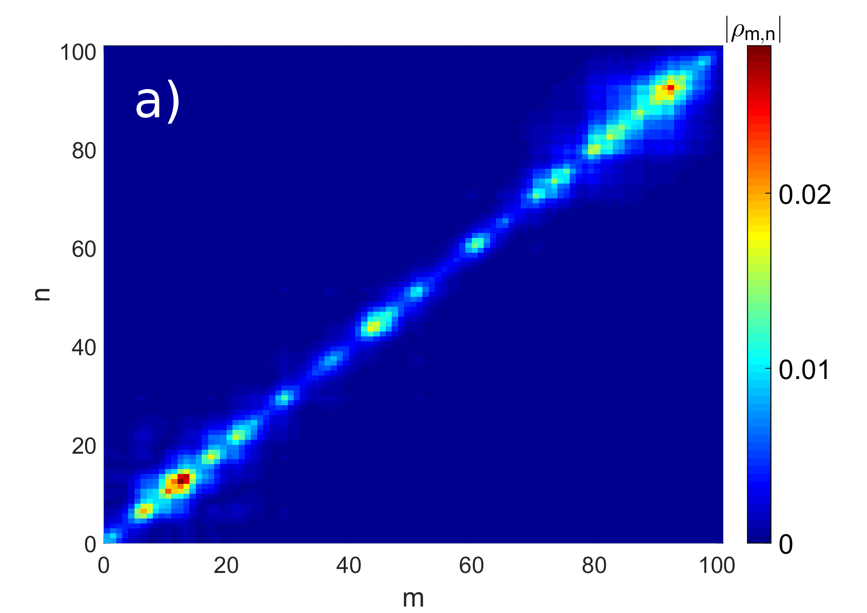
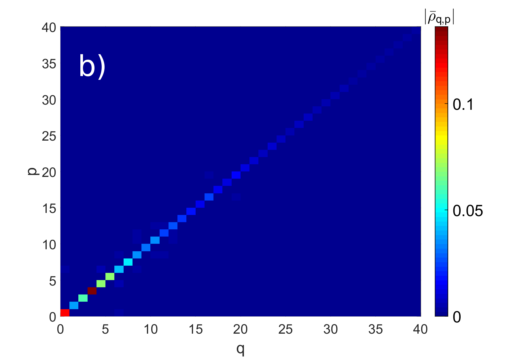
Figure 1: Absolute values of the elements of the asymptotic density matrix $\varrho_{\infty}$ expressed in (a) the original basis and (b) the basis of the Anderson modes (a relevant part is shown) for a particular disorder realization of the model system, Eqs. (1-3), and in-phase next-neighbor dissipators, $\alpha=0$ and $l=1$ in Eq. (4). Other parameters are $W=1$, $N=100$, and $\gamma=0.1$.

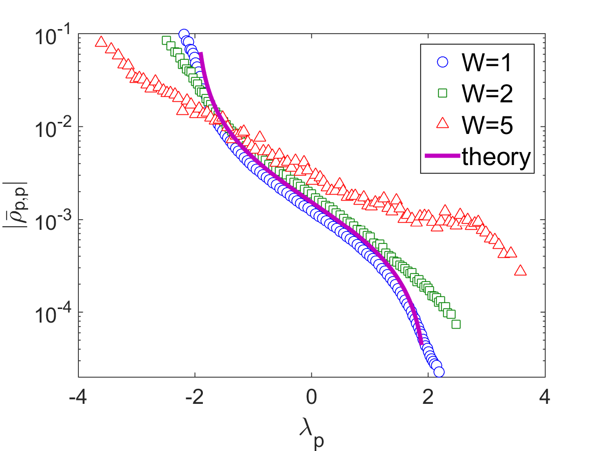
Figure 2: Averaged absolute values at the diagonal of $\varrho_{\infty}$, expressed in the Anderson basis, as functions of averaged eigenvalues for the case of in-phase next-neighbor dissipation, $\alpha=0$ and $l=1$ in Eq. (4). Averaging was performed over $N_{\mathrm{r}}=10^{2}$ disorder realizations. Theoretical prediction, Eq. (9), is shown by a thick solid line. The other parameters are the same as in Fig. 1.

We consider an open single-particle model described by Eq. (1) with a Hamiltonian anderson

$$H= \sum_{k}\epsilon_{k}b_{k}^{\dagger}b_{k}-(b_{k}^{\dagger}b_{k+1}+b_{k+1}^{\dagger}b_{k}),$$ (3)

where $\epsilon_{k}\in\left[-W/2,W/2\right]$ are random uncorrelated on-site energies, $W$ is the disorder strength, $b_{k}$ and $b_{k}^{\dagger}$ are the annihilation and creation operators of a boson on the $k$-th site. We recall that the eigenvalues of the Hamiltonian are restricted to a finite interval, $\lambda_{\nu}\in\left[-2-W/2,2+W/2\right]$, while the respective eigenstates, $A_{k}^{(\nu)}$, are exponentially localized. The localization length is approximated by $\xi_{\lambda}\approx 24(4-\lambda^{2})/W^{2}$ Thouless1979 with corrections about the band edges Derrida .

A single dissipative operator acts on a pair of sites,

$$V_{k}=(b_{k}^{\dagger}+e^{i\alpha}b_{k+l}^{\dagger})(b_{k}-e^{-i\alpha}b_{k+l}).$$ (4)

When $\alpha=0$, this operator tries to synchronize the dynamics on the $k$ and $k+l$ sites, by constantly recycling anti-symmetric out-of-phase mode into the symmetric in-phase one. This type of dissipation, with $l=1$, was introduced in Refs. DiehlZoller2008 ; KrausZoller . A physical implementation of a Bose-Hubbard chain with neighboring sites coupled by such dissipators was discussed in Ref.  marcos2012 . The proposed set-up consists of an array of superconductive resonators coupled by qubits; a pair-wise dissipator with $l=1$ and arbitrary phase $\alpha$ can be realized with the same set-up by (i) varying the photonic mode frequency $\omega_{k}$ from cavity to cavity (to simulate the disorder), and (ii) adjusting position of the qubits with respect to the centers of the corresponding cavities adja . In principle, this is enough for our purpose. However, to address other possible implementations, we will consider also dissipators with $l>1$.

Next we assume $\varrho_{0}=\varrho_{N+1}=0$ at the boundaries and analyze properties of the stationary solution $\varrho_{\infty}$ of Eq. (1), which is unique due to the absence of relevant symmetries alicki ; symmetry . To find it, we use a column-wise vectorization of the density matrix and define the asymptotic solution, a super-vector $\rho_{\infty}$, as the kernel of a Liouvillian-induced super-operator $\Pi$, $\Pi\rho_{\infty}=0$. After folding it into the matrix form and trace-normalizing, we get the asymptotic state density matrix $\varrho_{\infty}$ exact .

For the choice $\alpha=0$ and $l=1$ in Eq. (4), that is the case of in-phase next-neighbor dissipative coupling DiehlZoller2008 ; KrausZoller ; marcos2012 , the asymptotic density matrix exhibits a patchy structure with several ’hot’ localization spots, Fig. 1a. Remarkably, expressing the density operator in the basis of Anderson modes $A_{\nu}$, we get a near diagonal matrix with a strong contributions from the eigenstates from the lower part of the spectrum, Fig. 1b.

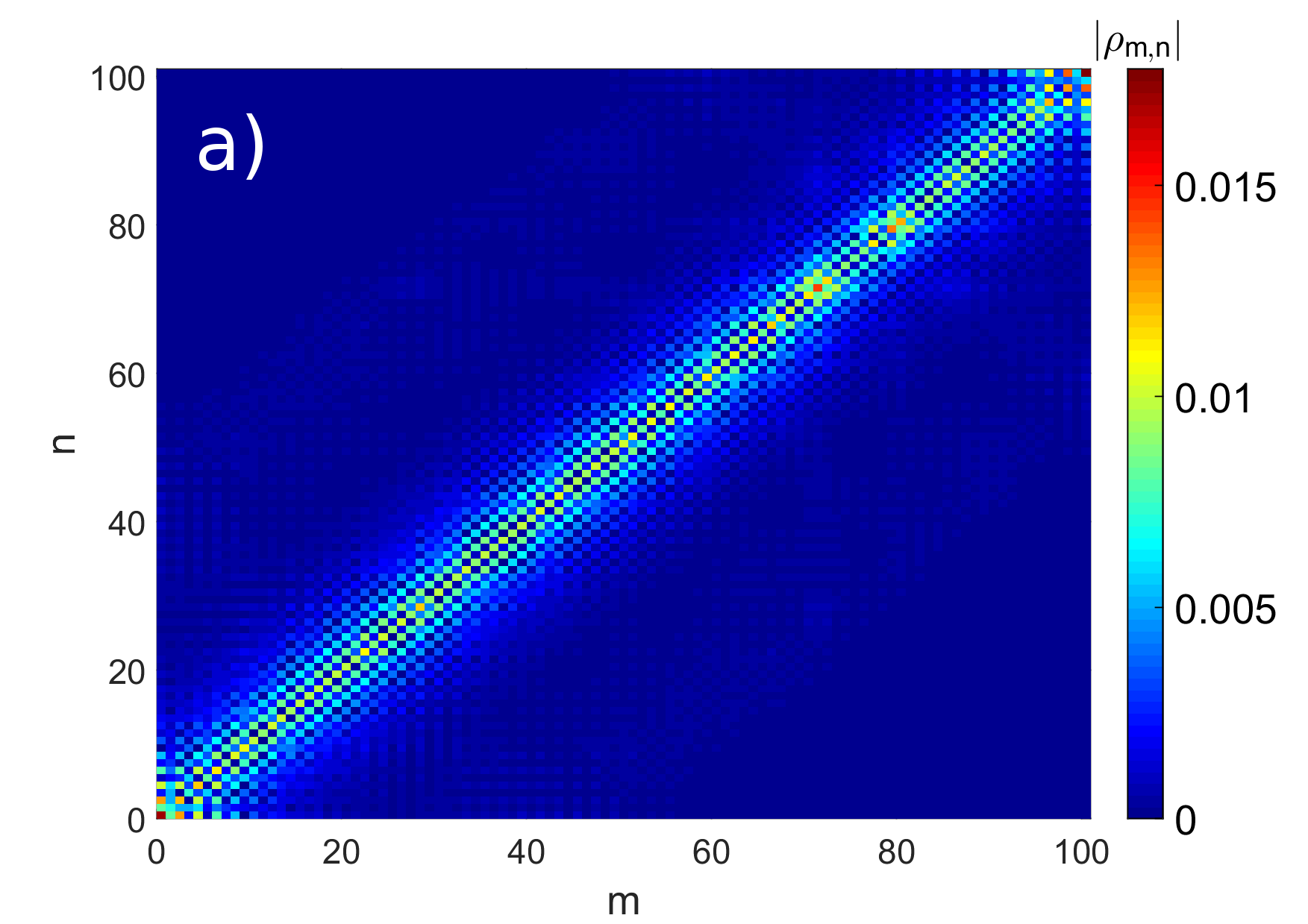
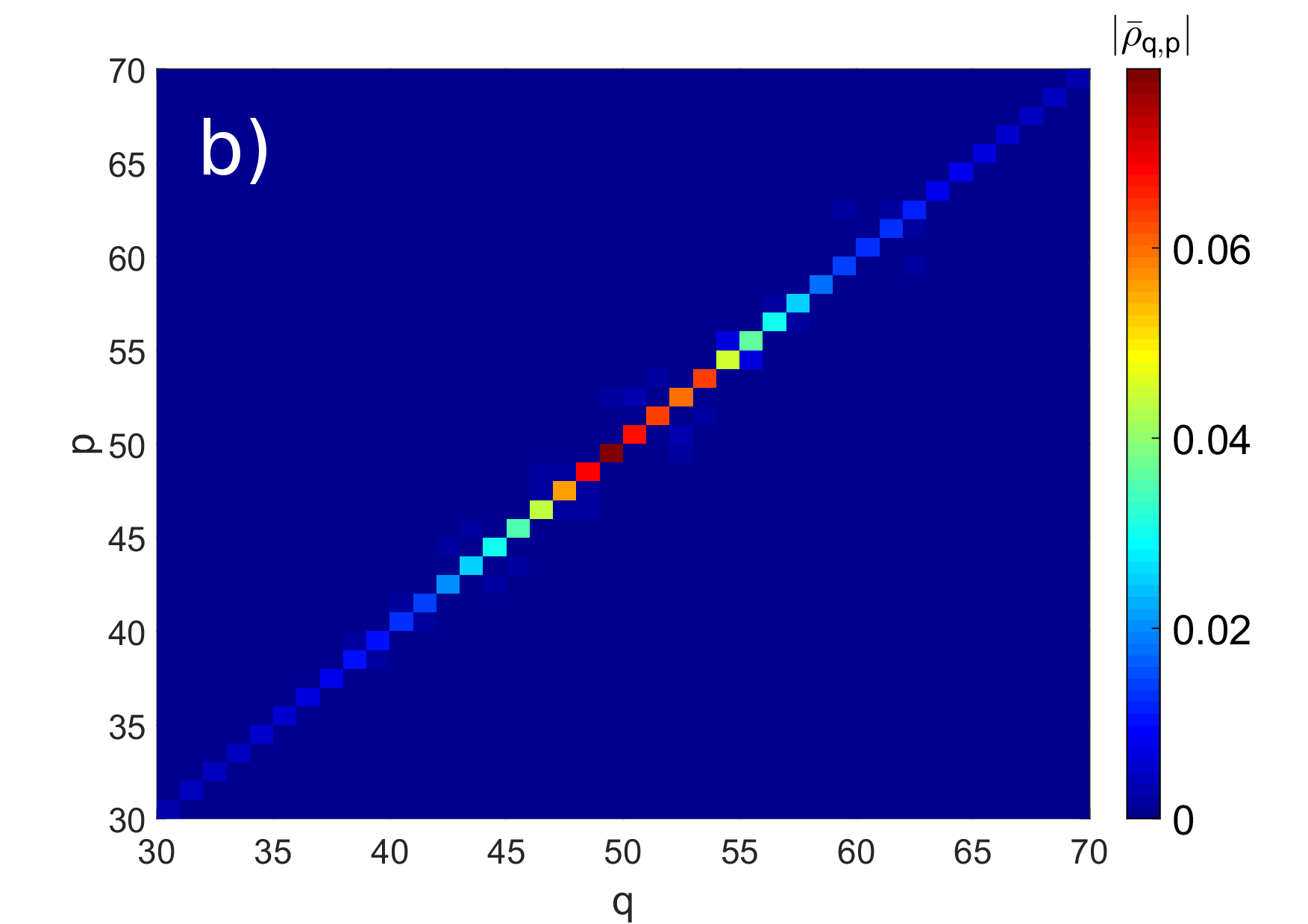
Figure 3: (a) Absolute values of the elements of the stationary density matrix $\varrho_{\infty}$ in the direct basis and (b) the basis of the Anderson modes (a relevant part is shown) for a particular disorder realization of the model, Eqs. (1-3), and out-of-phase next-nearest-neighbor dissipators, $\alpha=\pi$ and $l=2$ in Eq. (4). Other parameters are $W=1$, $N=100$, $\gamma=0.1$.

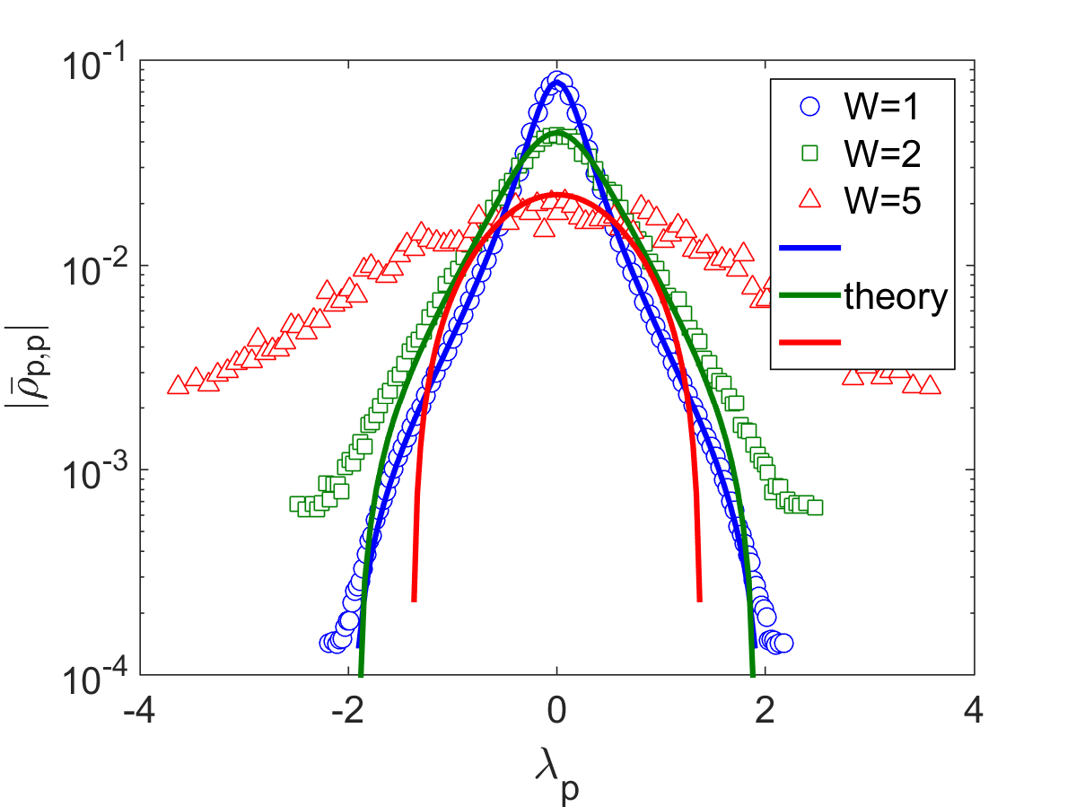
Figure 4: Averaged absolute values of the diagonal elements of $\varrho_{\infty}$, expressed in the Anderson basis, as functions of average eigenvalues for the case of out-of-phase next-nearest-neighbor dissipator, $\alpha=\pi$ and $l=2$ in Eq. (4). Averaging was performed over $N_{\mathrm{r}}=10^{2}$ disorder realizations. Theoretical predictions, Eq. (9), are shown by thick solid lines. Other parameters are $N=100$, $\gamma=0.1$.

To evaluate this finding analytically, we rewrite Eq. (1) in the Anderson basis and neglect the off-diagonal elements. Under this approximation, the evolution of the diagonal elements is governed by dissipative terms only,

$$\dot{\bar{\varrho}}_{p,p}=\gamma\left(\sum_{q}I_{p,q}\bar{\varrho}_{q,q}-\bar{\varrho}_{p,p}\sum_{q}I_{q,p}\right),$$ (5)

where the overlap coefficients $I_{p,q}=\sum_{k}|(\bar{V}_{k})_{q,p}|^{2}$ are given by the dissipators in the Anderson basis, $\{\bar{V}_{k}\}$. Explicitly,

$$I_{p,q}=\sum_{k}\left(A_{p,k+l}+e^{i\alpha}A_{p,k}\right)^{2}\left(A_{q,k+l}-e^{-i\alpha}A_{q,l}\right)^{2}.$$ (6)

Denoting $I_{p,k}^{\pm}=\left(A_{p,k+l}\pm e^{\pm i\alpha}A_{p,k}\right)^{2}$, we obtain for the stationary solution:

$$\bar{\varrho}_{p,p}=\frac{\sum_{k}I_{p,k}^{+}\sum_{q}I_{q,k}^{-}\bar{\varrho}_{q,q}}{\sum_{k}I_{p,k}^{-}\sum_{q}I_{q,k}^{+}}.$$ (7)

The inner sums in the numerator and denominator do not depend on the index $p$, and subjected to the averaging over all eigenstates spanned by $q$. Because the disorder is spatially homogeneous, the ensemble average makes the result also $k$-independent and so it corresponds to a normalization constant. With that we arrive at the following expression for the asymptotic density matrix:

$$\bar{\varrho}_{p,p}\propto\frac{\sum_{k}I_{p,k}^{+}}{\sum_{k}I_{p,k}^{-}}=\frac{I_{p}^{+}}{I_{p}^{-}},$$ (8)

which is fully determined by the type of dissipation and a spatial structure of a particular Anderson eigenstate.

For in-phase next-neighbor dissipators, $\alpha=0$ and $l=1$ in Eq. (4), it follows $\sum_{k}\left(A_{p,k+1}\pm A_{p,k}\right)^{2}=2\pm 2\sum_{k}A_{p,k+1}A_{p,k}=2\mp\lambda_{p}\mp\sum\epsilon_{k}A_{p,k}^{2}$ explain . Except for the case of strong localization ($\xi_{p}\sim 1$, for $W>4$ or about the band edges), the last term averages out due to spatial disorder and can therefore be neglected, and so we end up with

$$\bar{\varrho}_{p,p}\propto\frac{2-\lambda_{p}}{2+\lambda_{p}},$$ (9)

This result explains the quick decay of the contribution from the eigenstates away from the lower band edge. We numerically calculate, for different disorder strengths, the average distribution of the diagonal elements of $\varrho_{\infty}$, expressed in the Anderson basis, and plot them as functions of the average eigenvalues, see Fig. 2. The obtained results are in a good agreement with the theoretical prediction, Eq. (9). Note that the mismatch increases with the disorder strength $W$ and near the band edges; these effects follow from the nature of the made approximations.

It is straightforward to see that in case of anti-phase next-neighbor dissipators, $\alpha=\pi$ and $l=1$, the symmetry of the problem leads to the inverse expression, $\bar{\varrho}_{p,p}\propto\frac{2+\lambda_{p}}{2-\lambda_{p}}$, and the asymptotic state localized near the upper band edge. A choice $\alpha=\pi/2$ makes all dissipative operators $V_{k}$, Eq. (4), Hermitian. This leads to the complete delocalization of the asymptotic state, $\varrho_{\infty}=\mathbb{1}/N$. Intermediate phase values, $0<\alpha<\pi/2$ ($\pi/2<\alpha<\pi$), produce asympotic density matrix (expressed in the Anderson basis) with dominating diagonal elements localized near the lower (upper) band edge.

A qualitatively different picture is observed with next nearest neighbor dissipators, $\alpha=\pi$ and $l=2$. In this case the asymptotic state becomes delocalized in the original basis, Fig. 3a. At the same time, it remains localized in the Anderson basis, though shifted to the center of the spectrum, see Fig. 3b. Delocalization in the direct space occurs due to the substantial spatial overlap of the contributing Anderson states, which are much weaker localized at the band center than at the edges. Analytically, that corresponds to $I_{p}^{-}=\sum_{k}\left(A_{p,k+2}+A_{p,k}\right)^{2}=\lambda_{p}^{2}-2\lambda_{p}\sum_{k}\epsilon_{k}A_{p,k}A_{p,k+1}+\sum_{k}\epsilon_{k}^{2}A_{p,k}^{2}\approx\lambda_{p}^{2}+W^{2}/12$ and $I_{p}^{+}=4-I_{p}^{-}$, and it follows

$$\bar{\varrho}_{p,p}\propto\frac{4}{\lambda_{p}^{2}+W^{2}/12}-1.$$ (10)

This expression indicates that the dominant contribution comes from the central Anderson modes. We also calculate the average profiles of asymptotic states for different disorder strengths to compare them with the analytical solution, which depends now explicitly on $W$, Fig. 4. Again, we find a good agreement with the numerical results, while the mismatch increases with $W$ and distance from the band center.

Is is noteworthy that in the limit of strong localization, $W\gg 1$, when all eigenstates are essentially single-site localized, dissipation induces strong delocalization. As it follows from Eq. (6), in this limit all overlap coefficients become $I_{p,q}\sim\delta_{p,q}$, and the distribution of the values of the diagonal elements of the density matrix expressed in the Anderson basis should become near uniform. This means also delocalization in the direct space. As disorder strength increases, this trend can be seen on both Figs. 2 and 4.

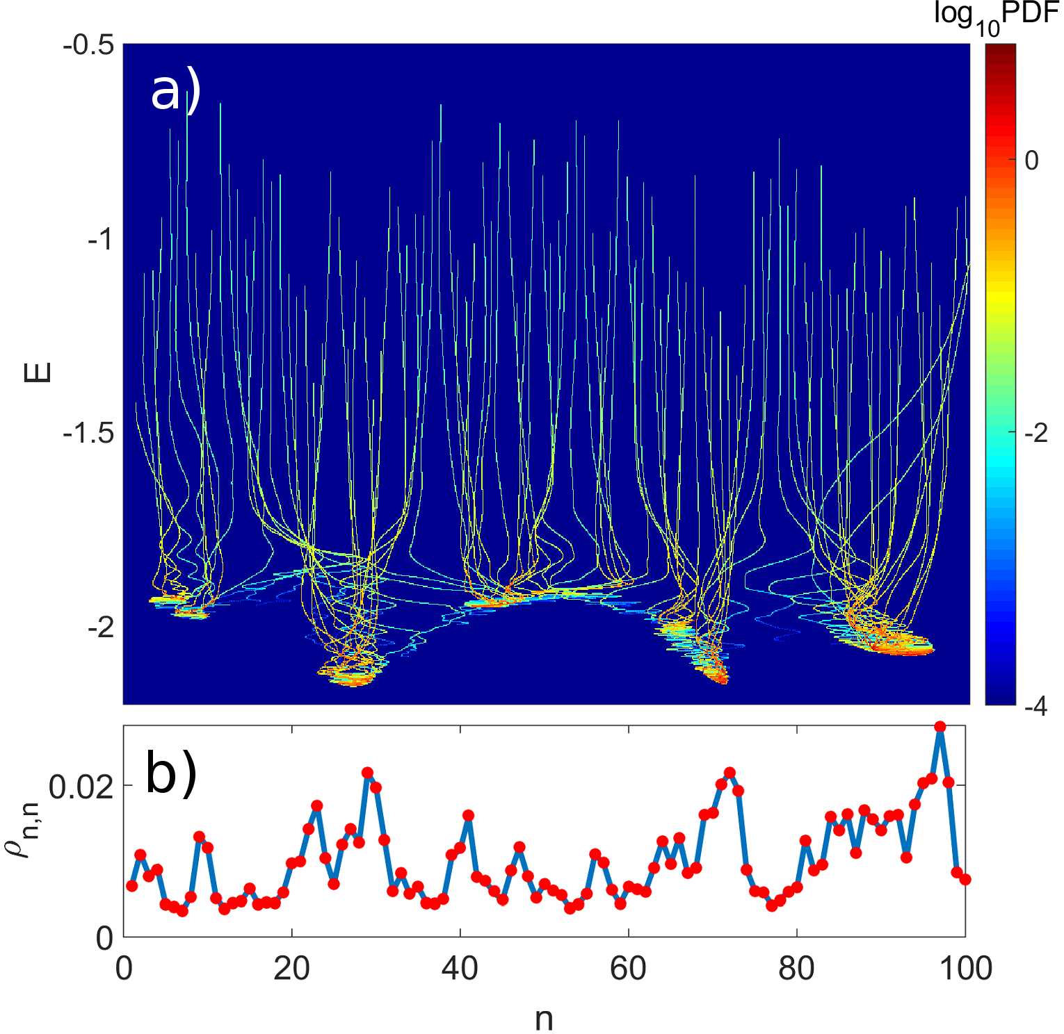
Figure 5: (a) Probability density function on the position-energy plane for quantum trajectories in the asymptotic regime; (b) The diagonal elements of the stationary density matrix (expressed in the direct basis) obtained as the stationary solution of Eq. (1) (blue solid line) and as the marginal distribution of the above probability density function (red dots). The pdf was obtained with $M_{\mathrm{r}}=10^{6}$ trajectories and transients time $t_{\mathrm{tr}}=10^{4}$. Other parameters are $W=1,\gamma=0.1,N=100,\alpha=0$, and $l=1$.

We gain further insight in the dissipative effects by unraveling deterministic equation (1) into an ensemble of quantum trajectories plenio ; dali ; zoller1992 . This allows us to recast the evolution of the model system in terms of pure states, governed by an effective non-Hermitian Hamiltonian, $\tilde{H}=H-\frac{i}{2}\sum_{k}V^{\dagger}_{k}V_{k}$, and random jumps induced by dissipators $V_{k}$. This is not a formal step only; for some quantum optics realizations it may properly model the reality of the experiment plenio . For $W=1,\gamma=0.1$ and $N=100$, we choose transient time $t_{\mathrm{tr}}=10^{4}$ and performed an averaging over $M_{\mathrm{r}}=10^{6}$ realizations to calculate the probability density function (pdf) on the position-energy plane, $\{n(t)=\sum_{k}\langle\psi(t)|n_{k}|\psi(t)\rangle$ and $E(t)=\langle\psi(t)|H|\psi(t)\rangle\}$.

Figure 5(a) presents the obtained pdf for the case of in-phase next-neighbor dissipators, $\alpha=0$ and $l=1$. On the trajectory level, the asymptotic dynamics of the system is remarkable. Several localized states are selected from the part of the spectrum specified by the phase properties of dissipators (here it is the lower band edge). The intermittent dynamics is a mixture of sticky-like beating near one of the localized eigenstates (non-Hermitian evolution with $\tilde{H}$ Fyodorov ), which are interrupted by quantum jumps (induced by a randomly selected operator $V_{k}$). Every jump throws the system into the high-energy region from where it quickly relaxes, through a fine-structured network, to one of the eigenstates. The structure of the network is specific to the disorder realization; however, it does not change with further increase of $M_{\mathrm{r}}$. Marginal distribution over $n(t)$ recovers the diagonal elements of the asymptotic density matrix $\varrho_{\infty}$ expressed in the direct basis, see Fig. 5b.

We have shown that dissipation can be used to create steady states dominated by a few localized modes of a spatially disordered Hamiltonian. Anderson modes are selected according to their spatial-phase properties inherited from the seeding plane waves, the eigenstates of the Hamiltonian in the zero-disorder limit ishii , by using phase-parametrized dissipative operators. It is possible to steer the system into a desired asymptotic state, with footprints of localization or completely delocalized, by changing phase parameter of the dissipative operators.

Our findings pose several interesting issues for future investigations. First, it is a synergy between dissipation and modulation effects, such as dynamical localization RefA1 . A quantum chaos, induced by strong periodic modulations RefA2 ; RefA3 ; RefA5 ; RefA6 ; RefA4 or quasi-periodic modulations RefA7 , can also play a role of an effective disorder and lead to AL-like effects. A controllable dissipation, added to such systems, can lead to nontrivial results. Next direction is many-body localization Basko , a phenomenon actively explored now. What could be a result of the interplay of dissipation and many body localization fish ; les ; les2 when the dissipative operators are phase-contolled? It is possible to create a MBL steady state with local dissipators? To answer these questions, not only spectra of the MBL Hamiltonians and such integral characteristics as, e.g., the inverse participation ratio, have to be analyzed, but also spatial phase structure of MBL eigenstates.

Acknowledgments: This work was supported by the Russian Science Foundation grant No. 15-12-20029.

References

- (1) B. Kramer and A. MacKinnon, Rep. Prog. Phys. 56, 1469 (1993).
- (2) F. Evers and A. Mirlin, Rev. Mod. Phys. 80, 1355 (2008).
- (3) 50 Years of Anderson Localization, ed. by E. Abrahams (World Scientific, 2010).
- (4) A. Lagendijk, B. van Tiggelen, and D. S. Wiersma, Physics Today 62, 24 (2009).
- (5) M. Segev, Y. Silberberg, and D. N. Christodoulides, Nature Photon. 7, 197 (2013).
- (6) J. Billy, V. Josse, Z. Zuo, A. Bernard, B. Hambrecht, P. Lugan, D. Clément, L. Sanchez-Palencia, P. Bouyer, and A. Aspect, Nature 453, 891 (2008).
- (7) G. Roati, C. D’Errico, L. Fallani, M. Fattori, C. Fort, M. Zaccanti, G. Modugno, M. Modugno, and M. Inguscio, Nature 453, 895 (2008).
- (8) S. S. Kondov, W. R. McGehee, J. J. Zirbel, B. DeMarco, Science 334, 66 (2011).
- (9) F. Jendrzejewski, A. Bernard, K. Müller, P. Cheinet, V. Josse, M. Piraud, L. Pezzé, L. Sanchez-Palencia, A. Aspect, and P. Bouyer, Nature Phys. 8, 398 (2012).
- (10) H.-P. Breuer, F. Petruccione, The Theory of Open Quantum Systems (Oxford University Press, Oxford, 2002).
- (11) S. Diehl, A. Micheli, A. Kantian, B. Kraus, H. P. Büchler, P. Zoller, Nature Physics 4, 878 (2008).
- (12) B. Kraus H. P. Büchler, S. Diehl, A. Kantian, A. Micheli, P. Zoller, Phys. Rev. A 78, 042307 (2008).
- (13) F. Verstraete, M. M. Wolf, and J.I. Cirac, Nature Phys. 5, 633 (2009).
- (14) D. Valenti, L. Magazzú, P. Caldara, and B. Spagnolo, Phys. Rev. B 91, 235412 (2015).
- (15) L. Magazzú, D. Valenti, B. Spagnolo, and M. Grifoni, Phys. Rev. E 92, 032123 (2015).
- (16) L. Magazzú, A. Carollo, B. Spagnolo, D. Valenti, J. of Stat. Mech. 054016 (2016).
- (17) N. Syassen, D.M. Bauer, M. Lettner, T. Volz, D. Dietze, J. J. Garcia-Ripoll, J. I. Cirac, G. Rempe, S. Dürr, Science, 320, 1329 (2008).
- (18) D. Witthaut, F. Trimborn, and S. Wimberger Phys. Rev. Lett. 101, 200402 (2008).
- (19) D. Witthaut, F. Trimborn, H. Hennig, G. Kordas, T. Geisel, and S. Wimberger, Phys. Rev. A 83, 063608 (2011).
- (20) G. Kordas, S. Wimberger, and D. Witthaut, Phys. Rev. A 87, 043618 (2013).
- (21) P. W. Anderson, Phys. Rev. 109, 1492 (1958).
- (22) P. Stano and P. Jacquod, Nature Photonics 7, 66 (2013).
- (23) J. Liu, P. D. Garcia, S. Ek, N. Gregersen, T. Suhr, M. Schubert, J. Mørk, S. Stobbe, and P. Lodahl, Nat. Nanotech. 9, 285 (2014).
- (24) T. V. Laptyeva, A. A. Tikhomirov, O. I. Kanakov and M. V. Ivanchenko, Sci. Rep. 5, 13263 (2015).
- (25) T. V. Laptyeva, S. V. Denisov, G. V. Osipov, M. V. JETP Lett., 102 (9), 603 (2015).
- (26) S. Genway, I. Lesanovsky, and J. P. Garrahan, Phys. Rev. E 89, 042129 (2014)
- (27) R. Alicki, K. Lendi, 1987, Quantum Dynamical Semigroups and Applications, Lecture Notes in Physics, Vol. 286 (Springer, Berlin).
- (28) M. F. Fisher, M. Maksymenko, E. Altman, Phys. Rev. Lett. 116, 160401 (2016).
- (29) E. Levi, M. Heyl, I. Lesanovsky, J. P. Garrahan, Phys. Rev. Lett. 116, 237203 (2015).
- (30) B. Everest, I. Lesanovsky, J. P. Garrahan, E. Levi, arXiv:1605.07019 (2016).
- (31) C. E. Bardyn, M. A. Baranov, C. V. Kraus, E. Rico, A. İmamoǵlu, P. Zoller, and S. Diehl, New. J. Phys. 15, 085001 (2013).
- (32) J. T. Barreiro, M. Müller, P. Schindler, et. al., Nature Phys. 6, 943 (2010).
- (33) D. Kienzler, H.-Y. Lo, B. Keitch, L. de Clercq, F. Leupold, F. Lindenfelser, M. Marinelli, V. Negnevitsky, J. P. Home, Science 347 53 (2015).
- (34) D. Vorberg, W. Wustmann, R. Ketzmerick, A. Eckardt, Phys. Rev. Lett. 111, 240405 (2013).
- (35) D. Marcos, A. Tomadin, S. Diehl, and P. Rabl, New J. Phys. 15, 055005 (2012).
- (36) The relative position of a qubit in a cavity controls the phase of a complex coupling constant in the Jaynes-Cummings coupling term, , where qubit operator QO . To realize dissipator (4) with and in the set-up proposed in Ref. marcos2012 , the coupling constant should vary with as .
- (37) P. Meystre and M. Sargent, Elements of Quantum Optics (Springer, Berlin, 4 ed., 2007).
- (38) D. J. Thouless, In: Ill-condensed Matter, Eds. R. Balian, R. Maynard, and G. Toulouse (North-Holland, 1979).
- (39) B. Derrida and E. Gardner, J. Physique 45, 1283 (1984).
- (40) V. V. Albert, L. Jiang, Phys. Rev. A 89, 022118 (2014).
- (41) Maximal absolute value of the elements in the r.h.s of equation (1) after substituion of does not exceed .
- (42) S. Diehl, A. Tomadin, A. Micheli, R. Fazio, P. Zoller, Phys. Rev. Lett. 105, 015702 (2010).
- (43) The last step relies on the identity obtained from the eigenstate equation , multiplied by and summed over .
- (44) M. B. Plenio and P. L. Knight, Rev. Mod. Phys. 70, 101 (1998).
- (45) J. Dalibard, Y. Castin, and K. Mølmer, Phys. Rev. Lett. 68, 580 (1992);
- (46) R. Dum, A.S. Parkins, P. Zoller, and C.W. Gardiner, Phys. Rev. A 46, 4382 (1992).
- (47) Y. V. Fyodorov, JETP Letters 78, 250 (2003).
- (48) K. Ishii, Prog. Theor. Phys. Suppl. 53, 77 (1973).
- (49) S. Fishman, D. R. Grempel, and R. E. Prange, Phys. Rev. Lett. 49, 509 (1982).
- (50) S. Wimberger, A. Krug, and A. Buchleitner, Phys. Rev. Lett. 89, 263601 (2002).
- (51) F. Jörder, K. Zimmermann, A. Rodriguez, and A. Buchleitner, Phys. Rev. Lett. 113, 063004 (2014).
- (52) J. E. Bayfield, G. Casati, I. Guarneri, and D.W. Sokol, Phys. Rev. Lett. 63, 364 (1989).
- (53) C. F. Bharucha, J.C. Robinson, F. L. Moore, B. Sundaram, Q. Niu, and M.G. Raizen, Phys. Rev. E 60, 3881 (1999).
- (54) E. J. Galvez, B. E. Sauer, L. Moorman, P. M. Koch, and D. Richards, Phys. Rev. Lett. 61, 2011 (1988).
- (55) J. Chabé, G. Lemarié, B. Grémaud, D. Delande, P. Szriftgiser, and J. C. Garreau, Phys. Rev. Lett. 101, 255702 (2008).
- (56) D. M. Basko, I. L. Aleiner and B. L. Altshuler, Ann. Phys. 321, 1126 (2006).