Randomized Incremental Construction for the Hausdorff Voronoi Diagram revisited and extended

Abstract

The Hausdorff Voronoi diagram of clusters of points in the plane is a generalization of Voronoi diagrams based on the Hausdorff distance function. Its combinatorial complexity is $O(n+m)$, where $n$ is the total number of points and $m$ is the number of crossings between the input clusters ($m=O(n^{2})$); the number of clusters is $k$. We present efficient algorithms to construct this diagram following the randomized incremental construction (RIC) framework [Clarkson et al. 89, 93]. Our algorithm for non-crossing clusters ($m=0$) runs in expected $O(n\log{n}+k\log n\log k)$ time and deterministic $O(n)$ space. The algorithm for arbitrary clusters runs in expected $O((m+n\log{k})\log{n})$ time and $O(m+n\log{k})$ space. The two algorithms can be combined in a crossing-oblivious scheme within the same bounds. We show how to apply the RIC framework to handle non-standard characteristics of generalized Voronoi diagrams, including sites (and bisectors) of non-constant complexity, sites that are not enclosed in their Voronoi regions, empty Voronoi regions, and finally, disconnected bisectors and disconnected Voronoi regions. The Hausdorff Voronoi diagram finds direct applications in VLSI CAD.

1 Introduction

The Voronoi diagram is a powerful geometric partitioning structure that finds diverse applications in science and engineering [2]. In this paper we consider the Hausdorff Voronoi diagram of clusters of points in the plane, a generalization of Voronoi diagrams based on the Hausdorff distance function, which has applications in predicting (and evaluating) faults in VLSI layouts and other geometric networks embedded in the plane.

Given a family $F$ of $k$ clusters of points in the plane, where the total number of points is $n$ ($n=|\cup F|$), the Hausdorff Voronoi diagram of $F$ is a subdivision of the plane into maximal regions such that all points within one region have the same nearest cluster (see Figure 1a). The distance between a point $t\in\mathbb{R}^{2}$ and a cluster $P\in F$ is measured by their Hausdorff distance, which equals the farthest distance between $t$ and $P$, $\textup{{d}}_{\textup{{f}}}(t,P)=\max_{p\in P}d(t,p)$ and $d(\cdot,\cdot)$ denotes the Euclidean distance between two points in the plane. No two clusters in $F$ share a common point.

Informally, the Hausdorff Voronoi diagram is a min-max type of diagram. The opposite max-min type, where distance is minimum and the diagram is farthest, is also of interest, see e.g., [8, 1, 14]. Recently both types of diagrams have been combined to determine stabbing circles for sets of line segments in the plane [11]. We remark that the Hausdorff diagram is different in nature from the clustering induced Voronoi diagram by Chen et al. [7], where sites can be all subsets of points and the influence function reflects a collective effect of all points in a site.

The Hausdorff Voronoi diagram finds direct applications in Very Large Scale Integration (VLSI) circuit design. It can be used to model the location of defects falling over parts of a network that have been embedded in the plane, destroying its connectivity. It has been used extensively by the semiconductor industry to estimate the critical area of a VLSI layout for various types of open faults, see e.g., [18, 5]. Critical area is a measure reflecting the sensitivity of a design to random manufacturing defects. The diagram can find applications in geometric networks embedded in the plane, such as transportation networks, where critical area may need to be extracted for the purpose of flow control and disaster avoidance.

Previous work.

The Hausdorff Voronoi diagram was first considered by Edelsbrunner et al. [13] under the name cluster Voronoi diagram. The authors showed that its combinatorial complexity is $O(n^{2}\alpha(n))$, and gave a divide and conquer construction algorithm of the same time complexity, where $\alpha(n)$ is the inverse Ackermann function. These bounds were later improved to $O(n^{2})$ by Papadopoulou and Lee [20]. When the convex hulls of the clusters are disjoint [13] or non-crossing (see Definition 1) [20], the combinatorial complexity of the diagram is $O(n)$. The $O(n^{2})$-time algorithm of Edelsbrunner et al. is optimal in the worst case. It exploits the equivalence of the Hausdorff diagram to the upper envelope of a family of $k$ lower envelopes (one for each cluster) in an arrangement of planes in $\mathbb{R}^{3}$. However, it remains quadratic even if the diagram has complexity $O(n)$. To continue our description, we need the following.

Definition 1

Two clusters $P$ and $Q$ are called non-crossing, if the convex hull of $P\cup Q$ admits at most two supporting line segments with one endpoint in $P$ and one endpoint in $Q$. If the convex hull of $P\cup Q$ admits more than two such supporting segments, then $P$ and $Q$ are called crossing (see Figure 1b).

The combinatorial complexity of the Hausdorff Voronoi diagram is $O(n+m)$, where $m$ is the number of crossings between pairs of crossing clusters (see Definition 2), and this is tight [19]. The number of crossings $m$ is upper-bounded by the number of supporting segments between pairs of crossing clusters. In the worst case, $m$ is $\Theta(n^{2})$. Computing the Hausdorff Voronoi diagram in subquadratic time when $m$ is $O(n)$ (even if $m=0$) has not been an easy task. For non-crossing clusters ($m=0$), the Hausdorff Voronoi diagram is an instance of abstract Voronoi diagrams [15]. But a bisector can have complexity $\Theta(n)$, thus, if we directly apply the randomized incremental construction for abstract Voronoi diagrams [16] we get an $O(n^{2}\log n)$-time algorithm, and this is not easy to overcome (see [6]). When clusters are crossing, their bisectors are disconnected curves [20], and thus, they do not satisfy the basic axioms of abstract Voronoi diagrams.

For non-crossing clusters, Dehne et al. [12] gave the first subquadratic-time algorithm to compute the Hausdorff diagram, in time $O(n\log^{5}n)$ and space $O(n\log^{2}n)$. Recently, Cheilaris et al. presented a randomized incremental construction for this problem, which is based on point location in a hierarchical dynamic data structure [6]. The expected running time of this algorithm is $O(n\log{n}\log{k})$ and the expected space complexity is $O(n)$ [6]. However, this approach does not easily generalize to crossing clusters.

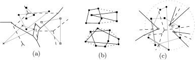
Figure 1: (a) The Hausdorff Voronoi diagram of a family of four clusters, where each cluster contains three points. (b) A pair of clusters. Above: clusters are non-crossing; below: clusters are crossing. (c) Two crossing clusters $P$ and $Q$ (filled disks and squares, resp.), and their Hausdorff Voronoi diagram (black lines). The region of $P$ is disconnected into three faces. A crossing mixed vertex $v$, the circle passing through the three points that induce $v$ (dotted lines), and two diagonals of $P$ and $Q$ related to $v$ (bold, grey).

Our Contribution.

In this paper we revisit the randomized incremental construction for the Hausdorff diagram and obtain three new results, which complete our investigation on randomized incremental construction algorithms for this diagram. The obtained results are especially relevant to the setting driven by our application, where crossings may be present whose number is expected to be small (typically, $m=O(n)$). We follow the randomized incremental construction (RIC) framework introduced by Clarkson et al. [9, 10]. We show how to efficiently apply this framework to construct a generalized Voronoi diagram in the presence of several non-standard features: (1) bisectors between pairs of sites can each have complexity $\Theta(n)$; (2) sites need not be enclosed in their Voronoi regions; (3) Voronoi regions can be empty; and (4) bisector curves may be disconnected. Note that a direct application of the framework would yield an $O(n^{2}\log n)$ (or $O(kn\log n)$) -time algorithm, even for a diagram of complexity $O(n)$.

First, we consider non-crossing clusters, for which the complexity of the diagram is $O(n)$. Our algorithm runs in expected $O(n\log{n}+k\log{n\log{k}})$ time and deterministic $O(n)$ space. In comparison to our previous algorithm [6], the construction is considerably simpler and it slightly improves its time complexity. We give the construction for both a conflict and a history graph, where the latter is an on-line variation of the algorithm (see Section 3.3).

Then, we consider arbitrary clusters of points. Allowing clusters to cross adds an entire new challenge to the construction algorithm: a bisector between two clusters consists of multiple connected components, thus, one Voronoi region may disconnect in several faces. We show how to overcome this challenge on a conflict graph and derive an algorithm whose expected time and space requirements are respectively $O(m\log{n}+n\log{k}\log{n})$ and $O(m+n\log{k})$. To the best of our knowledge, this is the first time the RIC framework is applied to the construction of a Voronoi diagram with disconnected bisectors and disconnected regions.

Finally, we address the question of deciding which algorithm to use on a given input, without a prior knowledge on the existence of crossings. Deciding whether the input clusters are crossing (or not) may require quadratic time by itself, because the convex hulls of the input clusters may have quadratic number of intersections, even if the clusters are non-crossing. In Section 5, we show how to only detect crossings that are relevant to the construction of the Hausdorff Voronoi diagram, and thus, provide a crossing-oblivious algorithm that combines our two previous algorithms, while keeping intact the time complexity bounds.

2 Preliminaries

Let $F$ be a family of $k$ clusters of points in the plane, and let $n$ be the total number of points in $F$; no two clusters share a point. We assume that each cluster equals the vertices on its convex hull, as only points on a convex hull may have non-empty regions in the Hausdorff Voronoi diagram. For simplicity of presentation, we follow a general position assumption that no four points lie on the same circle. This general position assumption can be removed similarly to an ordinary Voronoi diagram of points, e.g., following techniques of symbolic perturbation [21].

The farthest Voronoi diagram of a cluster $C$, for brevity $\textup{{FVD}}(C)$, is a partitioning of the plane into regions such that the farthest Voronoi region of a point $c\in C$ is

$$\textup{{freg}}_{C}(c)=\{t\mid\forall c^{\prime}\in C\setminus\{c\}\colon d(t,c)>d(t,c^{\prime})\}.$$

Let ${\mathcal{T}}(C)$ denote the graph structure of $\textup{{FVD}}(C)$, ${\mathcal{T}}(C)=\mathbb{R}^{2}\setminus\bigcup_{c\in C}\textup{{freg}}_{C}(c)$. If $|C|>1$, ${\mathcal{T}}(C)$ is well known to be a tree; we assume that ${\mathcal{T}}(C)$ is rooted at a point at infinity on an arbitrary unbounded Voronoi edge. If $C=\{c\}$, let ${\mathcal{T}}(C)=c$.

The Hausdorff Voronoi diagram, for brevity $\textup{{HVD}}(F)$, is a partitioning of the plane into regions such that the Hausdorff Voronoi region of a cluster $C\in F$ is

$$\textup{{hreg}}_{F}(C)=\{p\mid\forall C^{\prime}\in F\setminus\{C\}\colon\textup{{d}}_{\textup{{f}}}(p,C)<\textup{{d}}_{\textup{{f}}}(p,C^{\prime})\}.$$

The region $\textup{{hreg}}_{F}(C)$ is further subdivided into subregions by the $\textup{{FVD}}(C)$. In particular, the Hausdorff Voronoi region of a point $c\in C$ is

$$\textup{{hreg}}_{F}(c)=\textup{{hreg}}_{F}(C)\cap\textup{{freg}}_{C}(c).$$

Figure 1a illustrates the Hausdorff Voronoi diagram of a family of four clusters, where the convex hulls of the clusters are shown in grey lines. Solid black lines indicate the Hausdorff Voronoi edges bounding the regions of individual clusters, and the dashed lines indicate the finer subdivision, which is induced by the farthest Voronoi diagram of each cluster. Figure 1c illustrates the diagram for a different faily of clusters following the same drawing conventions.

The Hausdorff Voronoi edges are portions of Hausdorff bisectors between pairs of clusters. The Hausdorff bisector of two clusters $P,Q\in F$ is $\textup{{b}}_{\textup{{h}}}(P,Q)=\{y\mid\textup{{d}}_{\textup{{f}}}(y,P)=\textup{{d}}_{\textup{{f}}}(y,Q)\}$; see the solid black lines in Figure 1c. It is a subgraph of ${\mathcal{T}}(P\cup Q)$, and it consists of one (if $P,Q$ are non-crossing) or more (if $P,Q$ are crossing) unbounded polygonal chains [20]. In Figure 1c the Hausdorff bisector of the two clusters has three such chains. Each vertex of $\textup{{b}}_{\textup{{h}}}(P,Q)$ is the center of a circle passing through two points of one cluster and one point of another, which entirely encloses $P$ and $Q$, see, e.g., the dotted circle with center at vertex $v$ in Figure 1c.

Definition 2

A vertex on the bisector $\textup{{b}}_{\textup{{h}}}(C,P)$, induced by two points $c_{i},c_{j}\in C$ and a point $p_{l}\in P$, is called crossing, if there is a diagonal $p_{l}p_{r}$ of $P$ that crosses the diagonal $c_{i}c_{j}$ of $C$, and all points $c_{i},c_{j},p_{l},p_{r}$ are on the convex hull of $C\cup P$. (See vertex $v$ in Figure 1c.) The total number of crossing vertices along the bisectors of all pairs of clusters is the number of crossings and this is denoted by $m$.

The Hausdorff Voronoi diagram contains three types of vertices [19] (see Figures 1a and c): (1) pure Voronoi vertices, equidistant to three clusters; (2) mixed Voronoi vertices, equidistant to three points of two clusters; and (3) farthest Voronoi vertices, equidistant to three points of one cluster. The mixed vertices, which are induced by two points of cluster $C$ (and one point of another cluster), are called $C$-mixed vertices, and they are incident to edges of $\textup{{FVD}}(C)$. The Hausdorff Voronoi edges are polygonal lines (portions of Hausdorff bisectors) that connect pure Voronoi vertices. Mixed Voronoi vertices are vertices of Hausdorff bisectors. They are characterized as crossing or non-crossing according to Definition 2. The following property is crucial for our algorithms.

Lemma 1 ([19])

Each face of a (non-empty) region $\textup{{hreg}}_{F}(C)$ intersects ${\mathcal{T}}(C)$ in one non-empty connected component. The intersection points delimiting this component are $C$-mixed vertices.

Unless stated otherwise, we use a refinement of the Hausdorff Voronoi diagram as derived by the visibility decomposition of each region $\textup{{hreg}}_{F}(p)$ [20] (see Figure 2a): for each vertex $v$ on the boundary of $\textup{{hreg}}_{F}(p)$ draw the line segment $p{v}$, as restricted within $\textup{{hreg}}_{F}(p)$. Each face $f$ within $\textup{{hreg}}_{F}(p)$ is convex. In Figure 2a, the edges of the visibility decomposition in $\textup{{hreg}}_{F}(p)$ are shown in bold.

Observation 1

A face $f$ of $\textup{{hreg}}_{F}(p)$, $p\in P$, borders the regions of $O(1)$ (at most 3) other clusters in $F\setminus\{P\}$.

Given a cluster $P$ and its farthest Voronoi diagram $\textup{{FVD}}(P)$, our algorithms often need to answer the following query, termed the segment query:

Definition 3 (Segment Query [6])

Given two clusters $P,C\in F$, $\textup{{FVD}}(P)$, and a line segment $uv\subset{\mathcal{T}}(C)$ such that $\textup{{d}}_{\textup{{f}}}(u,C)<\textup{{d}}_{\textup{{f}}}(u,P)$ and $\textup{{d}}_{\textup{{f}}}(v,C)>\textup{{d}}_{\textup{{f}}}(v,P)$, find the point $x\in uv$ that is equidistant to $C$ and $P$.

Following [6], this query can be answered in $O(\log{|P|})$ time using the centroid decomposition of $\textup{{FVD}}(P)$, see [6] and references therein. The centroid decomposition of $\textup{{FVD}}(P)$ is obtained by recursively breaking ${\mathcal{T}}(P)$ into subtrees of its centroid, where the centroid of a tree with $h$ vertices is a vertex whose removal decomposes the tree into subtrees with at most $h/2$ vertices each.

Overview of the RIC framework [9, 10].

The framework of the randomized incremental construction (RIC) to compute a Voronoi diagram, inserts sites (also called objects) one by one, in random order, each time recomputing the target diagram. The diagram is viewed as a collection of ranges (also called regions), defined and without conflicts with respect to the set of sites inserted so far. To update the diagram efficiently after each insertion, a conflict or a history graph is maintained. An important prerequisite for using the framework is that each range must be defined by a constant number of objects.

The conflict graph is a bipartite graph, where one group of nodes corresponds to the ranges of the diagram defined by the sites inserted so far, and the other group corresponds to sites that have not yet been inserted. In the conflict graph, a range and a site are connected by an arc if and only if they are in conflict. A RIC algorithm using a conflict graph is efficient if the following update condition is satisfied at each incremental step: (1) Updating the set of ranges defined and without conflicts over the current subset of objects requires time proportional to the number of ranges deleted or created during this step; and (2) Updating the conflict graph requires time proportional to the number of arcs of the conflict graph that are added or removed during this step.

The expected time and space complexity for a RIC algorithm is as stated in [4, Theorem 5.2.3]: Let $f_{0}(r)$ be the expected number of ranges in the target diagram of a random sample of $r$ objects, and let $k$ be the number of insertion steps of the algorithm. Then: (1)  The expected number of ranges created during the algorithm is $O\left(\sum\limits_{r=1}^{k}(f_{0}(r)/r)\right)$. (2) If the update condition holds, the expected time and space of the algorithm is $O\left(k\sum\limits_{r=1}^{k}(f_{0}(r)/r^{2})\right)$.

The history graph is a directed acyclic graph defined as follows. At each step of the algorithm, the nodes of the history graph correspond to all ranges created by the algorithm so far. The nodes with zero out-degree, termed leaf nodes, correspond to the ranges present in the current target diagram. The nodes that have outgoing edges, termed intermediate nodes, correspond to the ranges that have been deleted already. Intermediate nodes are connected, by their outgoing edges, to the nodes whose insertion caused the deletion of their ranges. The latter nodes are referred to as the children of the former nodes. The update condition for a history graph is the following: (i) The out-degree of each node is bounded by a constant; and (ii) the existence of a conflict between a given range and a given object can be tested in constant time. The bounds on the time complexity of a randomized incremental algorithm using a history graph are the same as those given in item (2) above; the storage required by the algorithm equals the number of ranges created during the algorithm and its expected value is bounded as in item (1) above.

The rest of the paper is organized as follows. In Section 3 we give an algorithm to construct $\textup{{HVD}}(F)$ for the input cluster families where all clusters are pairwise non-crossing. In Section 4 we give an algorithm for the inputs where clusters may be crossing. Both algorithms follow the RIC framework (with the conflict graph) reviewed in the above paragraphs, therefore each of the two sections consists of: (1) the definition of objects, ranges and conflicts, (2) the procedure to insert an object and to update the conflict graph, and (3) the analysis of time and space complexity (note that the analysis differs substantially from simply applying ready theorems about RIC). In addition, Section 3 contains an adaptation of the algorithm to work with history graph instead of the conflict graph; this adaptation in turn follows the above presentation scheme of three items (1)-(3). Finally, in Section 5 we show how to combine the algorithm of Section 3 and the one of Section 4 in an efficient algorithm for the case where it is not known whether the input clusters have crossings.

3 Constructing $\textup{{HVD}}(F)$ for non-crossing clusters

Let the clusters in the input family $F$ be pairwise non-crossing. Then each Voronoi region is connected and the combinatorial complexity of the Hausdorff Voronoi diagram is $O(n)$.

(a)

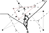
(b)

(c)

Figure 2: Left: (a) Visibility decomposition of the diagram. Right: Insertion of a cluster $C$ (unfilled disks): (b) ${\mathcal{T}}(C)$ (dashed) rooted at $r$, its active subtree (bold) rooted at $x$. (c) After the insertion: $x$ is a $C$-mixed vertex of the HVD.

Let $S\subset F$ such that $\textup{{HVD}}(S)$ has been computed. Let $C\in F\setminus S$; our goal is to insert $C$ and obtain $\textup{{HVD}}(S\cup\{C\})$. We first introduce the following definition for an active subtree of ${\mathcal{T}}(C)$ and its root.

Definition 4

Traverse ${\mathcal{T}}(C)$, starting at its root, and let $x$ be the first point we encounter in the closure of $\textup{{hreg}}_{S\cup\{C\}}(C)$. We refer to the subtree of ${\mathcal{T}}(C)$ rooted at $x$ as the active subtree of ${\mathcal{T}}(C)$ and denote it by $\mathcal{T}_{a}(C,S)$. Let $x$ be the root of $\mathcal{T}_{a}(C,S)$.

Note that the roots of ${\mathcal{T}}(C)$ and $\mathcal{T}_{a}(C,S)$ may coincide, in which case, $\mathcal{T}_{a}(C,S)={\mathcal{T}}(C)$. In Figure 2b, $\mathcal{T}_{a}(C,S)$ is shown in bold dashed lines superimposed on $\textup{{HVD}}(S)$. Figure 2c illustrates $\textup{{HVD}}(S\cup\{C\})$. By Lemma 1, and since the Voronoi regions of non-crossing clusters are connected, we have the following property.

Property 1

The region $\textup{{hreg}}_{S\cup\{C\}}(C)\neq\emptyset$ if and only if $\mathcal{T}_{a}(C,S)\neq\emptyset$. The root of $\mathcal{T}_{a}(C,S)$ is a $C$-mixed vertex of $\textup{{HVD}}(S\cup\{C\})$ (unless $\mathcal{T}_{a}(C,S)={\mathcal{T}}(C)$).

3.1 Objects, ranges and conflicts

We formulate the problem of computing $\textup{{HVD}}(F)$ in terms of objects, ranges and conflicts, see Section 2. The objects are clusters in $F$. The ranges are the refined faces of $\textup{{HVD}}(S)$, as refined by the visibility decomposition of $\textup{{HVD}}(S)$ (see Section 2 and Figure 1c). A range corresponding to a face $f$, where $f\subset\textup{{hreg}}_{S}(p)$ and $p\in P$, is said to be defined by the cluster $P$ and by the remaining clusters in $S$ whose Voronoi regions border $f$. By Observation 1, there are at most three such clusters; thus, the RIC framework is applicable. Point $p$ is called the owner of range $f$ and $\textup{{hreg}}_{S}(p)$.

Definition 5 (Conflict for non-crossing clusters)

A range $f$ is in conflict with a cluster $C\in F\setminus S$, if $\mathcal{T}_{a}(C,S)$ is not empty and its root $x$ lies in $f$. A conflict is a triple $(f,x,C)$; the list of conflicts of range $f$ is denoted by $\mathcal{L}(f)$.

The following property is implied by Lemma 1. It is essential for our algorithm.

Lemma 2

Each cluster in $F\setminus S$ has at most one conflict with the ranges in $\textup{{HVD}}(S)$. If a cluster $C\in F\setminus S$ has no conflicts, then $\textup{{hreg}}_{S\cup\{C\}}(C)=\emptyset$, thus, $\textup{{hreg}}_{F}(C)=\emptyset$.

In the following section, we present the variant of our algorithm, i.e., the procedure to insert a cluster, that is based on a conflict graph. In Section 3.3, we present an adaptation using a history graph.

3.2 Insertion of a cluster

Suppose that $\textup{{HVD}}(S)$, $S\subset F$, and its conflict graph with $F\setminus S$ have been constructed. Let $C\in F\setminus S$. Using the conflict of $C$, we can easily compute $\textup{{hreg}}_{S\cup\{C\}}(C)$. Starting at the root of $\mathcal{T}_{a}(C,S)$ (which is stored with the conflict), trace the region boundary in an ordinary way  [20]. The main problem that remains is to identify the conflicts for the new ranges of $\textup{{hreg}}_{S\cup\{C\}}(C)$ and update the conflict graph. We give the algorithm to perform these tasks in Figure 3 as pseudocode and summarize it in the sequel.

To identify new conflicts we use the information stored with the ranges that get deleted. Let $f$ be a deleted range, and let $p$ be its owner ($f\subset\textup{{hreg}}_{S}(p)$). For each conflict $(f,y,Q)$ of $f$, where $Q$ is a cluster in $F\setminus S$ and $y$ is the root of $\mathcal{T}_{a}(Q,S)$, we compute the new root of $\mathcal{T}_{a}(Q,S\cup\{C\})$, if different from $y$, and identify the new range that contains it. To compute the root of $\mathcal{T}_{a}(Q,S\cup\{C\})$, it is enough to traverse $\mathcal{T}_{a}(Q,S)$, searching for an edge $uv$ that contains a point equidistant from $Q$ and $C$ (see Line 12 in Figure 3). If such an edge $uv$ exists, we perform a segment query in $\textup{{FVD}}(C)$ (see Definition 3), to compute the point equidistant from $C$ and $Q$ on $uv$ (a $Q$-mixed vertex) If no such edge exists, then $\mathcal{T}_{a}(Q,S\cup\{C\})=\emptyset$ and no conflicts for $Q$ should be created. The remaining algorithm is straightforward (see Figure 3). Its correctness is shown in the following lemma.

Figure 3: Algorithm to insert cluster $C$; case of non-crossing clusters.

Lemma 3

The algorithm Insert-NonCrossing (Figure 3) is correct.

Proof

The algorithm Insert-NonCrossing, to insert a cluster $C$, processes the unique conflict $(g,x,C)$ of cluster $C$. Having point $x$ as a starting point for tracing the boundary of $\textup{{hreg}}_{s\cup\{C\}}(C)$ (Line 2) is correct, since $x$ lies on that boundary as implied by Definition 5. The Clarkson-Shor framework [9, 10] (see also Section 2) implies that processing the conflicts of every deleted range (the loop in Lines 4–16) is enough for repairing the conflict graph. The only non-trivial parts of this loop are: the condition in Line 8, and handling of its two possible outcomes respectively in Lines 9–10 and Lines 12–17.

In Line 8, it is enough to compare the distance from $y$ to only $p$ and $C$ because no other cluster may become the closest to $y$ as a result of inserting $C$. Therefore by checking the condition in Line 8, we find out whether the owner of the face containing point $y$ in $\textup{{HVD}}(S\cup\{C\})$ stays the same as in $\textup{{HVD}}(S)$, or $y$ actually belongs to the new region $\textup{{hreg}}_{s\cup\{C\}}(C)$. The correctness of Lines 9–10, i.e, the case when point $y$ stays in the region of $p$, is easy to see. Suppose that $\textup{{d}}_{\textup{{f}}}(y,C)<\textup{{d}}_{\textup{{f}}}(y,Q)=\textup{{d}}_{\textup{{f}}}(y,p)$, and that $\mathcal{T}_{a}(Q,S\cup\{C\})\neq\emptyset$ (Lines 12–17). In this case $y$ is no longer a part of the (updated) diagram $\textup{{HVD}}(S\cup\{C\})$. Clearly, $\mathcal{T}_{a}(Q,S\cup\{C\})$ is a subtree of $\mathcal{T}_{a}(Q,S)$, thus, there is exactly one edge $uv$ of $\mathcal{T}_{a}(Q,S)$ such that $u\not\in\mathcal{T}_{a}(Q,S\cup\{C\})$ and $v\in\mathcal{T}_{a}(Q,S\cup\{C\})$. Edge $uv$ satisfies the condition of Line 12 by definition of an active subtree (see Definition 4). The root of an active subtree cannot coincide with a vertex of ${\mathcal{T}}(C)$ due to the general position assumption. Note that if we had no general position assumption, the root of an active subtree could coincide with a vertex of ${\mathcal{T}}(C)$, but this simple case can be easily detected in Line 12 by checking whether the vertices of ${\mathcal{T}}(C)$ visited by the search are equidistant to $Q$ and to $C$. ∎

The main result of this section is the following theorem, which we prove in the remaining part of this section.

Theorem 3.1

The Hausdorff Voronoi diagram of $k$ non-crossing clusters of total complexity $n$ can be computed in expected $O(n\log{n}+k\log{n}\log{k})$ time and deterministic $O(n)$ space.

Consider a random permutation $\{C_{1},\dots,C_{k}\}$ of the input family $F$, and the sequence $\{F_{0},\dots,F_{k}\}$, where $F_{0}=\emptyset$, $F_{i}=F_{i-1}\cup\{C_{i}\}$ and $F_{k}=F$.

At step $i$ we insert cluster $C_{i}$ by performing the algorithm Insert-NonCrossing (Figure 3). However, the update condition of the RIC framework does not hold, thus, we cannot directly use it to obtain the time complexity of our algorithm. To bound the expected total time required for updating the diagram, we use the analysis of [6], which applies to any randomized incremental construction algorithm for the Hausdorff Voronoi diagram, independently of the auxiliary data structure being used. The following lemma summarizes the result of [6].

Lemma 4 ([6])

During the course of a randomized incremental construction of the Hausdorff Voronoi diagram of a family of non-crossing clusters, the total expected number of updates made to the diagram is $O(n)$, and the total expected time required for updating the diagram is $O(n\log n)$, where $n$ is the total number of points in all clusters.

We now bound the work to update the conflict graph. We first give Lemmas 5–7, and then use them in Lemma 8 to derive this bound.

Lemma 5

The number of arcs in the conflict graph, at any step, is $O(k)$.

Proof

The statement is a direct implication of Lemma 2.

Lemma 6

Updating the conflict graph at step $i$ requires $O(\log{n}(N_{i}+R_{i}))$ time, where $N_{i}$ is the total number of edges dropped out of the active subtrees of clusters in $F\setminus F_{i}$ at step $i$, and $R_{i}$ is the total number of conflicts deleted at step $i$.

Proof

Updating the conflict graph corresponds to two nested for-loops in Lines 4–16 of the algorithm in Figure 3. Clearly the inner loop (Lines 6–15) is performed $O(R_{i})$ times in total. Inside this loop, a breadth-first search is performed that spends $O(\log{n})$ time per visited edge. By Lemma 2, one active subtree is considered at most once during one step. All the visited edges, except the last one, are dropped out of the respective active subtree. It remains to show, that, except for the breath-first search, the rest of the work in any execution of the inner loop requires $O(\log{n})$ time. Indeed, it is a point location in Line 8, a segment query in $\textup{{FVD}}(C_{i})$ in Line 13, a binary search in Line 9 or Line 15, and an insertion of a new conflict in Line 10 or Line 17. For information on the segment query, see Section 2. ∎

Lemma 7

The expected total number of conflicts deleted at step $i$ of the randomized incremental algorithm is $O(k/i)+D_{i}$, where $D_{i}$ is the number of clusters in $F\setminus F_{i}$ that used to have a conflict until step $i$, and do not have it any more.

Proof

Each conflict deleted at step $i$ either induces a conflict with a (new) range in $\textup{{HVD}}(F_{i})\setminus\textup{{HVD}}(F_{i-1})$, or the corresponding cluster is counted by $D_{i}$. Each cluster is counted at most once by $D_{i}$ due to Lemma 2. Thus, the total number of conflicts deleted at step $i$ equals the total number of conflicts of ranges inserted at step $i$ plus $D_{i}$. We bound the expectation of the former number by backwards analysis. After step $i$ is performed, the number of conflicts in the conflict graph is $O(k)$ by Lemma 5. Fix one conflict of some cluster $C_{k}$, $k\geq i$; it is between $C_{k}$ and a range of a cluster $C_{j}$, $j\leq i$; since the insertion order of clusters is random, the probability for $C_{j}$ to be inserted at step $i$ (i.e., to be $C_{i}$ in our notation) is $O(1/i)$. Summing this probability for all the conflicts, we obtain that the expected number of conflicts inserted at step $i$ is $O(k/i)$. ∎

Lemma 8

The expectation of the total time required to update the conflict graph throughout the algorithm is $O(n\log{n}+k\log{n}\log{k})$.

Proof

Summing the bound of Lemma 6 for all steps, we obtain that the total time required to update the conflict graph during all steps of the algorithm is $\sum\limits_{i=1}^{k}{O\left(\log{n}(N_{i}+R_{i})\right)}$. An edge of ${\mathcal{T}}(C)$ of any cluster $C\in F$ is dropped out from the active subtree of $C$ at most once. The total number of edges in the farthest Voronoi diagrams of all clusters in $F$ is $O(n)$. Thus the above sum is proportional to $O(\log{n})(n+\sum\limits_{i=1}^{k}{R_{i}})$. The expectation of this number is, by Lemma 7, $O\left(\left(n+\sum\limits_{i=1}^{k}\left({k{/}i+D_{i}}\right)\right)\log{n}\right)$. Note that $\sum\limits_{i=1}^{k}{D_{i}}\leq k$, since the active subtree of a cluster can become empty at most once. The claimed time complexity follows. ∎

We remark that the total number of conflicts created throughout our algorithm is $O(n+k\log k)$ (as evident by the proof of Lemma 8).

Proof (of Theorem 3.1)

The total expected time required for updating the diagram during all the steps of the algorithm is $O(n\log n)$ due to Lemma 4. The total expected time required for updating the conflict graph is $O(n\log{n}+k\log{n}\log{k})$ due to Lemma 8.

The space requirement at any step is proportional to the combinatorial complexity of the Hausdorff Voronoi diagram, which is $O(n)$, plus the total number of arcs of the conflict graph at this step, which is at most $k$ by Lemma 5. Hence the claimed $O(n)$ bound holds. ∎

3.3 Adapting the algorithm of Section 3 to using a history graph

Let $\mathcal{H}(F_{i})$ denote the history graph at step $i$ of the incremental algorithm. $\mathcal{H}(F_{0})$ is a single node that corresponds to the whole $\mathbb{R}^{2}$. For $i\in\{1,\dots,{k}\}$, $\mathcal{H}(F_{i})$ consists of all nodes and arcs of $\mathcal{H}(F_{i-1})$, and in addition it contains the following: (i) A node for each new range in $\textup{{HVD}}(F_{i})\setminus\textup{{HVD}}(F_{i-1})$. These nodes are called the nodes of level $i$. (ii) An arc connecting a deleted range $f\in\textup{{HVD}}(F_{i-1})\setminus\textup{{HVD}}(F_{i})$ to every new range $f^{\prime}\in\textup{{HVD}}(F_{i})\setminus\textup{{HVD}}(F_{i-1})$ such that $f^{\prime}$ intersects $f$.

Suppose that $\textup{{HVD}}(F_{i-1})$ and $\mathcal{H}(F_{i-1})$ have already been computed. To insert the next cluster $C_{i}$, we traverse $\mathcal{H}(F_{i-1})$ from root to a leaf. Simultaneously, we traverse ${\mathcal{T}}(C_{i})$, keeping track of the root $x$ of the active subtree $\mathcal{T}_{a}(C_{i},F_{j})$ at the current level $j$ of $\mathcal{H}(F_{i-1})$. When we reach a leaf of $\mathcal{H}(F_{i-1})$, we trace the boundary of the Voronoi region $\textup{{hreg}}_{F_{i}}(C_{i})$, starting at the root $x$ of $\mathcal{T}_{a}(C_{i},F_{i})$, and update $\mathcal{H}(F_{i-1})$ to become $\mathcal{H}(F_{i})$.

In detail, the procedure at level $j$ is as follows: Let $f$ be the face in $\textup{{HVD}}(F_{j})$ that contains the root $x$ of $\mathcal{T}_{a}(C_{i},F_{i})$. Suppose that $f$ is deleted at step $\ell$. If $\textup{{d}}_{\textup{{f}}}(x,C_{i})<\textup{{d}}_{\textup{{f}}}(x,C_{\ell})$, we search for the child $f^{\prime}$ of $f$, that has the same owner as $f$, and contains $x$; we move to the level $\ell$, keeping $x$ intact, and updating its face to be $f^{\prime}$. Else we search for the root $z$ of the (new) active subtree $\mathcal{T}_{a}(C_{i},F_{\ell}\cup\{C_{i}\})$ (the procedure to do this is the same as for the conflict graph, see Section 3.2). If $z$ is found, we move to level $\ell$, replace $x$ by $z$ and the face $f$ by $f^{\prime}\subset\textup{{hreg}}_{F_{\ell}}(C_{\ell})$ that contains $z$. If $z$ is not found, the active subtree $\textup{{hreg}}_{F_{i}}(C_{i})=\emptyset.$

Theorem 3.2

The Hausdorff Voronoi diagram of $k$ non-crossing clusters of total complexity $n$ can be computed by RIC with the history graph in expected $O(n\log{n}+k\log{n}\log{k})$ time and expected $O(n)$ space.

Proof

By Lemma 4, the total time required for updating the diagram during all steps of the algorithm is $O(n\log n)$. Lemma 4 also implies that the expected total number of ranges created during the algorithm is $O(n)$, which yields the bound on the expected storage requirement in the case of the history graph.

Updating the history graph during step $i$ takes time $O(\log{n}(N_{i}+K_{i}))$, where $N_{i}$ is the number of edges of ${\mathcal{T}}(C_{i})$ that do not belong to the active subtree $\mathcal{T}_{a}(C_{i},F_{i})$, and thus, they are eliminated by the breath-first search. $K_{i}$ is the number of clusters in the sequence $\{C_{1},\dots,C_{i-1}\}$ that change the root of the active subtree as we move in the history graph level by level. By the backwards analysis, the expectation of $K_{i}$ is $O(\log{i})$. Summing over all $k$ steps gives us $O(k\log{k})$. The total expected running time of the algorithm using the history graph is thus $O(n\log{n}+k\log{n}\log{k})$. ∎

4 Computing $\textup{{HVD}}(F)$ for arbitrary clusters of points

In this section we drop the assumption that clusters in the input family $F$ are pairwise non-crossing. This raises a major difficulty that Hausdorff bisectors may consist of more than one polygonal curve and Voronoi regions may be disconnected. The definition of conflict from Section 3.1 no longer guarantees a correct diagram. We thus need a new conflict definition. For a region $r\subset\mathbb{R}^{2}$, its boundary and its closure are denoted, respectively, $\partial r$ and $\overline{r}$.

Let $C_{1},\dots,C_{k}$ be a random permutation of clusters in $F$. We incrementally compute $\textup{{HVD}}(F_{i})$, $i=1,\ldots,k$, where $F_{i}=\{C_{1},C_{2},\dots,C_{i}\}$. At each step $i$, cluster $C_{i}$ is inserted in $\textup{{HVD}}(F_{i-1})$. We maintain the conflict graph (see Section 2) between the ranges of $\textup{{HVD}}(F_{i})$ and the clusters in $F\setminus F_{i}$. Like in Section 3, ranges correspond to faces of $\textup{{HVD}}(F_{i})$ as partitioned by the visibility decomposition.

When inserting cluster $C_{i}$, we compute $\textup{{hreg}}_{F_{i}}(C_{i})$, where $F_{i}=F_{i-1}\cup\{C_{i}\}$, using the information provided by the conflicts of $C_{i}$ with the ranges of $\textup{{HVD}}(F_{i-1})$. From these conflicts we must be able to find at least one point in each face of $\textup{{hreg}}_{F_{i}}(C_{i})$. For this purpose it is sufficient (by Lemma 1) that at every step $i$ of the algorithm, we maintain information on the $Q$-mixed vertices of $\textup{{HVD}}(F_{i}\cup\{Q\})$, for every $Q\in F\setminus F_{i}$. However, this is not sufficient to apply the Clarkson-Shor technique, since we need the ability to determine new conflicts from the conflicts of ranges that get deleted. Due to this requirement, it is essential that $Q$ is in conflict not only with the ranges of $\textup{{HVD}}(F_{i})$ that contain $Q$-mixed vertices in $\textup{{HVD}}(F_{i}\cup\{Q\})$, as Lemma 1 suggests, but also with all the ranges that intersect the boundary of $\textup{{hreg}}_{F_{i}\cup\{Q\}}(Q)$.

Let $f$ be a range of $\textup{{HVD}}(F_{i})$, $f\subset\textup{{hreg}}_{F_{i}}(p)$, where $p\in P$ and $P\in F_{i}$. Let $Q$ be a cluster in $F\setminus F_{i}$. We define a conflict between $f$ and $Q$ as follows.

Definition 6 (Conflict for arbitrary clusters)

Range $f$, $f\subset\textup{{hreg}}_{F_{i}}(p)$, is in conflict with cluster $Q$, if $f$ intersects the boundary of $\textup{{hreg}}_{F_{i}\cup\{Q\}}(Q)$. The vertex list $V(f,Q)$ of this conflict is the list of all vertices and all endpoints of $\textup{{b}}_{\textup{{h}}}(P,Q)\cap\overline{f}$, ordered in clockwise angular order around $p$.

The following observation is essential to efficiently update the conflict graph.

Observation 2

$\textup{{b}}_{\textup{{h}}}(P,Q)\cap\overline{f}=\textup{{b}}_{\textup{{h}}}(p,Q)\cap\overline{f}$. The order of vertices in the list $V(f,Q)$ coincides with the natural order of vertices along $\textup{{b}}_{\textup{{h}}}(p,Q)$.

Note that $\textup{{b}}_{\textup{{h}}}(p,Q)$ is a single convex chain [20], unlike $\textup{{b}}_{\textup{{h}}}(P,Q)$, and this is why it is much simpler to process the former chain rather than the latter. Figure 5 shows bisector $\textup{{b}}_{\textup{{h}}}(P,Q)$ and a range $f$ intersected by it. The boundary $\partial f$ of this range consists of four parts: the top side is a portion of a pure edge of $\textup{{HVD}}(F_{i})$; the bottom chain, shown in bold, is a portion of ${\mathcal{T}}(P)$; the two sides are edges of the visibility decomposition of $\textup{{hreg}}_{F_{i}}(p)$.

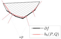
Figure 4: A range $f\subset\textup{{hreg}}_{F_{i}}(p)$ (shaded); Bisector $\textup{{b}}_{\textup{{h}}}(P,Q)$, $Q\in F\setminus F_{i}$; vertices of $\textup{{b}}_{\textup{{h}}}(P,Q)$ (unfilled circle marks).

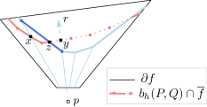
Figure 5: An old range $f\subset\textup{{hreg}}_{F_{i-1}}(p)$; New ranges of $\textup{{hreg}}_{F_{i}}(p)$ derived from $f$ (bounded by light solid lines). $\textup{{b}}_{\textup{{h}}}(P,Q)\cap\overline{f}$ where $Q$ is a cluster in conflict with $f$.

We proceed with a procedure to insert a cluser and to update the conflict graph after this insertion (see Section 4.1), and afterwards we analyze the complexity of this procedure and of the whole RIC algorithm (see Section 4.2).

4.1 Insertion of a cluster

Insert $C_{i}$ into $\textup{{HVD}}(F_{i-1})$.

We compute all faces of $\textup{{hreg}}_{F_{i}}(C_{i})$ by tracing their boundary, starting at the vertices in the vertex lists of the conflicts of $C_{i}$. In particular, while there are unprocessed vertices in these vertex lists, pick one such vertex $v$ and trace the connected component of $\partial\textup{{hreg}}_{F_{i}}(C_{i})$ adjacent to $v$. All vertices on that connected component are in the vertex lists of conflicts of $C_{i}$; mark them as processed.

The insertion of $\textup{{hreg}}_{F_{i}}(C_{i})$ results in deleting some ranges, which we call old ranges, and inserting some other ones, which we call new ranges. We have two types of new ranges: type (1): the ranges in $\textup{{hreg}}_{F_{i}}(C_{i})$; and type (2): the new ranges in the Hausdorff regions of clusters in $F_{i-1}$ derived from the old ranges, as a result of the insertion of $C_{i}$. The type (2) ranges are derived from the deleted ranges of clusters in $F_{i-1}$ (see Figure 5).

Update the conflict graph.

For each cluster $Q\in F\setminus F_{i}$ in conflict with at least one deleted range, compute the conflicts of $Q$ with the new ranges. We compute the conflicts with ranges of type (1) and (2) separately as follows.

Ranges of type (1).

Consider the ranges in $\textup{{hreg}}_{F_{i}}(C_{i})$. We follow the bisector $\textup{{b}}_{\textup{{h}}}(Q,C_{i})$ within $\textup{{hreg}}_{F_{i}}(C_{i})$, while computing this bisector on the fly. For each face $f\subset\textup{{hreg}}_{F_{i}}(C_{i})$ that is encountered as we walk on $\textup{{b}}_{\textup{{h}}}(Q,C_{i})$, we also discover vertices in $V(f,Q)$. Since $\textup{{b}}_{\textup{{h}}}(Q,C_{i})\cap f$ may consist of several components (see e.g. bold lines in Figure 5), $f$ can be encountered a number of times; each time, we augment $V(f,Q)$ independently. We do this by inserting in $V(f,Q)$ the vertices on the branch of $\textup{{b}}_{\textup{{h}}}(Q,C_{i})\cap f$ that had just been encountered, including its endpoints on $\partial f$. The position in $V(f,Q)$ of the insertion can be determined by binary search.

Ranges of type (2).

Let $f\subset\textup{{hreg}}_{F_{i-1}}(p)$, $p\in P$, be a deleted range that had been in conflict with $Q$. Recall that the vertex list $V(f,Q)$ corresponds to $\textup{{b}}_{\textup{{h}}}(P,Q)\cap\overline{f}$, which coincides with $\textup{{b}}_{\textup{{h}}}(p,Q)\cap\overline{f}$ (see Defintion 6 and Observation 2). In the following we always operate with the latter one. For each new range $f^{\prime}$ such that $f^{\prime}\subset f$ and $f^{\prime}$ is in conflict with $Q$, we need to compute list $V(f^{\prime},Q)$. Observe, that the union of $\textup{{b}}_{\textup{{h}}}(p,Q)\cap\overline{f^{\prime}}$, for all such ranges $f^{\prime}$, is $(\textup{{b}}_{\textup{{h}}}(p,Q)\cap\overline{f})\setminus\textup{{hreg}}_{F_{i}}(C_{i})$. We now introduce some notation.

We call the maximal contiguous portions of $\textup{{b}}_{\textup{{h}}}(p,Q)\cap\overline{f}$, outside $\textup{{hreg}}_{F_{i}}(C_{i})$, the active parts of $\textup{{b}}_{\textup{{h}}}(p,Q)\cap\overline{f}$. The non-active parts of $\textup{{b}}_{\textup{{h}}}(p,Q)\cap\overline{f}$ are its maximal contiguous portions inside $\textup{{hreg}}_{F_{i}}(C_{i})$. Figure 5 shows the active and the non-active parts of $\textup{{b}}_{\textup{{h}}}(p,Q)\cap\overline{f}$ by (red) bold and dotted lines respectively. Note that one active (resp., non-active) part may consist of multiple polygonal curves. A point incident to one active and one non-active part is called a transition point, see e.g. point $z$ in Figure 5.

Transition points lie in $\textup{{b}}_{\textup{{h}}}(Q,C_{i})\cap\partial\textup{{hreg}}_{F_{i}}(C_{i})$; they are used as starting points to compute conflicts for ranges of type (1). Our task is to determine all active parts of $\textup{{b}}_{\textup{{h}}}(p,Q)\cap\overline{f}$, their incident transition points, and to create conflicts induced by these active parts.

We process active and non-active parts of $\textup{{b}}_{\textup{{h}}}(p,Q)\cap\overline{f}$ sequentially:

• For a non-active part, we trace it in $\textup{{hreg}}_{F_{i}}(C_{i})$ in order to determine the transition point where the next active part begins.

• For an active part, we process sequentially the new ranges of $\textup{{HVD}}(F_{i})$ that are intersected by it. For each such range $f^{\prime}\subset f$, we compute $V(f^{\prime},Q)$, given the point $x$ where the active part enters $f^{\prime}$. In particular, we find the point $z$ where it exits $f^{\prime}$; after that the list $V(f^{\prime},Q)$ can be easily derived from the portion of $\textup{{b}}_{\textup{{h}}}(p,Q)$ between $x$ and $z$. A procedure to find point $z$ is detailed in Lemma 9. Point $z$ is the endpoint of the active part that we were processing, thus, $z$ is a transition point.

Lemma 9

Point $z$ can be determined in $O(\log{n})$ time.

Proof

To find point $z$, consider the rightmost ray $r$ originating at $p$ and passing through $\partial f^{\prime}$. If $\textup{{b}}_{\textup{{h}}}(p,Q)\cap\overline{f}$ intersects $r$ (see Figure 5), let $y$ be the point of this intersection. Otherwise, we let $t$ be the rightmost endpoint of $\textup{{b}}_{\textup{{h}}}(p,Q)\cap\overline{f}$ to the left of $r$. If $t\in{\mathcal{T}}(P)$, set $z=t$, otherwise set $y=t$.

If $y\in\partial f^{\prime}$, then we set $z=y$. In this case the active part of $\textup{{b}}_{\textup{{h}}}(p,Q)\cap\overline{f}$ enters the next new range $f^{\prime\prime}$ at point $y$. In Figure 5, this case is illustrated by point $x$ that plays the role of $z=y$.

If $y$ lies outside $\overline{f^{\prime}}$ ($y\not\in\overline{f^{\prime}}$), we determine point $z$ as the unique point on $\textup{{b}}_{\textup{{h}}}(p,Q)$, such that $z$ is between $x$ and $y$, and $z\in\partial f^{\prime}$. See Figure 5.

Suppose $y$ lies outside $\overline{f^{\prime}}$. In particular, by construction of $y$, it must lie in $\overline{f}\setminus\overline{f^{\prime}}$. The portion of $\textup{{b}}_{\textup{{h}}}(P,Q)$ between $x$ and $y$ lies entirely in $\overline{f}$, $x\in\overline{f^{\prime}}$, and $y\not\in\overline{f^{\prime}}$. By the visibility properties of $\textup{{b}}_{\textup{{h}}}(P,Q)$ and $\textup{{b}}_{\textup{{h}}}(P,C_{i})$, the portion of $\textup{{b}}_{\textup{{h}}}(P,Q)$ between $x$ and $y$ (excluding $x$) intersects $\partial f^{\prime}$ exactly once, and the intersection point $z$ lies on the top side of $\partial f^{\prime}$ (the portion of a pure edge of $\textup{{HVD}}(F_{i+1})$ on $\partial f^{\prime}$); see the dark blue line segment in Figure 5 or the top edge of $f$ in Figure 5. Let $ab$ denote the top side of $\partial f^{\prime}$, where $a$ precedes $b$ in the clockwise order around $p$. If $x\not\in ab$, the entire subsegment $az$ of $ab$ is closer to $Q$ than to $p$, and the entire $zb$ is closer to $p$ than to $Q$. If $x\in ab$, the above property holds for $xz$ and $zb$. Thus $z$ can be determined by a segment query for $ab$ (resp., $xb$) in $\textup{{FVD}}(Q)$ (see Definition 3 of the segment query). A segment query can be performed in $O(\log{n})$ time, see Section 2.

Points $y$ and $t$ can be found in $O(\log{n})$ time by a binary search in $V(f,Q)$. ∎

The following lemma shows correctness of the algorithm; its time and space complexity is analyzed in Section 4.2.

Lemma 10

The above algorithm correctly updates the Hausdorff Voronoi diagram and the conflict graph after insertion of $C_{i}$.

Proof

Correctness of updating the Hausdorff Voronoi diagram follows from Lemma 1. Indeed, each face of $\textup{{hreg}}_{F_{i}}(C_{i})$ is incident to at least one $C_{i}$-mixed vertex. Since all $C_{i}$-mixed vertices are in the vertex lists of the conflicts of $C_{i}$, all the faces of $\textup{{hreg}}_{F_{i}}(C_{i})$ are discovered.

While updating the conflict graph, all the conflicts between new ranges and clusters in $F\setminus F_{i}$ are computed. Indeed, for each $Q\in F\setminus F_{i}$, while computing the ranges of type (2), the algorithm discovers all the edges of $\textup{{HVD}}(F_{i}\cup{Q})$ outside $\textup{{hreg}}_{F_{i}}(C_{i})$. Using the transition points found while computing ranges of type (2) as starting points, the procedure to compute ranges of type (1) determines all the edges of $\textup{{HVD}}(F_{i}\cup{Q})$ inside $\textup{{hreg}}_{F_{i}}(C_{i})$. If it was not the case, then $Q$ would have a face in $\textup{{HVD}}(F_{i}\cup{Q})$ bounded solely by the edges induced by $C_{i}$ and $Q$, i.e., a face that lies inside the region of another cluster, which is not possible in the Hausdorff Voronoi diagram. ∎

4.2 Complexity analysis of the algorithm for arbitrary clusters

In this section we analyze the time and space complexity of the algorithm in Section 4.1. The conflicts are defined in a non-standard way, i.e., they have vertex lists whose complexity need not be constant. We use the Clarkson-Shor technique to bound the number of ranges created throughout the algorithm (see Theorem 3), but we cannot rely on the Clarkson-Shor technique to bound the total number of conflicts nor the time complexity of the algorithm, because the update condition of the technique (see Section 2) is not satisfied. Our analysis can be seen as extending the Clarkson-Shor analysis to such a non-standard setting.

In the next two lemmas, we analyze respectively the time complexity of updating the conflict graph after insertion of cluster $C_{i}$, and the total space required for the conflict graph at any step of the algorithm. The expectation of the total number of conflicts created during the algorithm is bounded in Theorem 4.1 that states the overall result.

Lemma 11

Updating the conflict graph after insertion of cluster $C_{i}$ can be done in time $O((A(C_{i})+L(C_{i})+V(C_{i}))\log{n})$, where $A(C_{i})$ is the number of conflicts created and deleted (i.e., new and old conflicts), $L(C_{i})$ is the total number of mixed vertices in the vertex lists of old conflicts that do not appear in the vertex lists of new conflicts, and $V(C_{i})$ is the total size of the vertex lists of all conflicts of all ranges of $\textup{{hreg}}_{F_{i}}(C_{i})$.

Proof

First consider the time complexity of creating all the conflicts of the new ranges derived from $\textup{{hreg}}_{F_{i}}(C_{i})$ (i.e., all the conflicts of the new ranges of type (1)). This is the total time spent for this task for all clusters $Q\in F\setminus F_{i}$ that are in conflict with such new ranges.

Tracing $\textup{{b}}_{\textup{{h}}}(Q,C_{i})$ inside $\textup{{hreg}}_{F_{i}}(C_{i})$ requires time proportional to the complexity of $\textup{{b}}_{\textup{{h}}}(Q,C_{i})\cap\textup{{hreg}}_{F_{i}}(C_{i})$, times $O(\log{n})$. The complexity of $\textup{{b}}_{\textup{{h}}}(Q,C_{i})\cap\textup{{hreg}}_{F_{i}}(C_{i})$ is the number of vertices of $\textup{{b}}_{\textup{{h}}}(Q,C_{i})\cap\textup{{hreg}}_{F_{i}}(C_{i})$ plus the number of times a boundary between two ranges of $\textup{{hreg}}_{F_{i}}(C_{i})$ was crossed by $\textup{{b}}_{\textup{{h}}}(Q,C_{i})$. This equals the total size of the vertex lists of all conflicts between $Q$ and the ranges of $\textup{{hreg}}_{F_{i}}(C_{i})$. Summing up this number for each cluster $Q$, we obtain $O(V(C_{i}))$. Thus the total time complexity of creating all the conflicts of the new ranges of type (1) is $O(V(C_{i})\log{n})$.

Now we analyze the time complexity of creating all the conflicts with the new ranges of type (2), for all clusters $Q\in F\setminus F_{i}$ that were in conflict with old ranges. The total time required for tracing the non-active parts of $\textup{{b}}_{\textup{{h}}}(p,Q)\in\overline{}f$ for all $Q$ is $O(L(C_{i})\log{n})$ similarly to the above, since all the conflicts corresponding to the non-active parts are discarded at this step.

What remains is to bound the time required for processing all the active parts of $\textup{{b}}_{\textup{{h}}}(p,Q)\in\overline{}f$ for all pairs $f,Q$ such that $f$ is an old range, and $Q$ was in conflict with $f$. Note that the vertices of the active parts of $\textup{{b}}_{\textup{{h}}}(p,Q)\in\overline{}f$ are counted neither by $L(C_{i})$ nor by $V(C_{i})$. To avoid visiting all vertices of the active parts and manipulating them explicitly, we do not store conflict lists together with conflicts, but rather we store them (united) with the owners of the corresponding ranges. In particular, at step $i$, for each point $p$ such that $\textup{{hreg}}_{F_{i}}(p)\neq\emptyset$, and each cluster $Q\in F\setminus F_{i}$ in conflict with some range of $\textup{{hreg}}_{F_{i}}(p)$, we store the list of vertices and endpoints of $\textup{{b}}_{\textup{{h}}}(p,Q)\cap\textup{{hreg}}_{F_{i}}(p)$, which is the union of $\textup{{b}}_{\textup{{h}}}(p,Q)\cap\overline{f}$ for all ranges $f$ of $\textup{{hreg}}_{F_{i}}(p)$. The conflict between $f$ and $Q$ then, instead of storing the list $V(f,Q)$, stores only the leftmost and the rightmost endpoints of $\textup{{b}}_{\textup{{h}}}(p,Q)\cap\overline{f}$. This way, the conflict between $Q$ and a new range $f^{\prime}$ of type (2), $f^{\prime}\subset\textup{{hreg}}_{F_{i}}(p)$, can be created in constant time, once the two endpoints of $\textup{{b}}_{\textup{{h}}}(p,Q)\cap\overline{f^{\prime}}$ are known. Any binary search in the list of vertices and endpoints of $\textup{{b}}_{\textup{{h}}}(p,Q)\cap\overline{f}$, e.g., the search for point $y$, can be performed in $O(\log{n})$ time.

To determine whether a given point $q\in f$ is in a new range of type (2) or not, it is enough to compare the distance from $q$ to the owner of $f$ and to cluster $C_{i}$. This is done by point location in $\textup{{FVD}}(C_{i})$, and thus requires $O(\log{n})$ time.

The total time required to create the conflicts of type (2) and to find the starting points for conflicts of type (1) is therefore $O((A(C_{i})+L(C_{i}))\log{n})$.

After all the new conflicts are created, for each deleted range $f$, we delete all the conflicts of $f$, which requires $O(A(C_{i}))$ time.

Finally, recall now that our procedure in fact creates first groups of smaller new ranges as subdivided by old ranges, and merges them in the true new ranges after their conflicts are computed. This requires additional $O(A(C_{i})\log n)$ time, since the total number of additional smaller new ranges is linear in the number of borders between old ranges, that is, $O(A(C_{i}))$. ∎

Lemma 12

At any step $i$, the total size of vertex lists of all the conflicts is $O(n+m+N_{i})$, where $N_{i}$ is the number of conflicts in the current conflict graph.

Proof

Consider a cluster $Q\in F\setminus F_{i}$. Members of the vertex lists of the conflicts of $Q$ are: (1) the mixed vertices of $\textup{{HVD}}(F_{i}\cup\{Q\})$ that bound the region of $Q$ in that diagram, $\textup{{hreg}}_{F_{i}\cup{Q}}(Q)$, and (2) points that are not mixed vertices of $\textup{{HVD}}(F_{i}\cup\{Q\})$. The total number of points of latter type is proportional to the number of conflicts of $Q$. Indeed, there are at most two points of the latter type per one conflict of $Q$ with a range $f$. Such points in $V(f,Q)$ are exactly the intersections between two polygonal chains, $\textup{{b}}_{\textup{{h}}}(p,Q)$ and $\partial f\setminus{\mathcal{T}}(P)$, where $p\in P$ and $f\subset\textup{{hreg}}_{F_{i}}(p)$. The first chain is concave (as seen from $p$), and the second one is convex. Thus they intersect in at most two points.

Now we bound the number of mixed vertices in the vertex lists of all conflicts of $Q$. Recall, that the mixed vertices in $V(f,Q)$ are $P$-mixed and $Q$-mixed vertices, where $P\in F_{i}$ is such that $f\subset\textup{{hreg}}_{F_{i}}(P)$. The total number of crossing mixed vertices in the vertex lists of all conflicts between $Q$ and ranges derived from the region of $P$ is linear in the number of crossings between $P$ and $Q$. There are at most two non-crossing $P$-mixed vertices in $V(f,Q)$ for each such conflict between $f$ and $Q$, since the boundary of $f$ that is a portion of ${\mathcal{T}}(P)$ is connected. The total number of $Q$-mixed vertices in $\textup{{HVD}}(F_{i}\cup\{Q\})$ is $O(|Q|)$. Thus the total number of mixed vertices in the vertex lists of all the conflicts of $Q$ is $O(|Q|+Cr(Q))$, where $Cr(Q)$ is the number of crossings between $Q$ and all the clusters in $F_{i}$.

The claim follows by summing up the above quantities over all clusters $Q$ in $F\setminus F_{i}$. ∎

We are now ready to state the main result of this section.

Theorem 4.1

The Hausdorff Voronoi diagram of a family $F$ of $k$ clusters of total complexity $n$ can be computed in $O((m+n\log{k})\log{n})$ expected time and $O(m+n\log{k})$ expected space.

Proof

The expected space complexity of the algorithm is $O(n\log{k}+m)$, implied by the fact that the Hausdorff Voronoi diagram of any subset of $F$ has complexity $O(n+m)$ [19], and by Lemma 12, stating that the additional space required to store vertex lists of the conflicts at each step is $O(n+m)$.

We now bound the expected time complexity of the algorithm. To this aim we estimate the expectation of the total number of conflicts created during the course of the algorithm, and the expectation of the sum of $L(C_{i})$ and of $V(C_{i})$, for $i=1,\dots,k$.

To analyze the expected total number of conflicts created during the course of the algorithm, we need to estimate the expected number of ranges, i.e., faces, in $\textup{{HVD}}(R)$, where $R$ is a random $r$-sample of $F$. The number of faces in a Hausdorff Voronoi diagram is proportional to the number of its mixed Voronoi vertices [19]. The number of non-crossing mixed vertices in $\textup{{HVD}}(R)$ is proportional to the total number of points in all clusters in $R$ [19]. The expectation of the latter number is $O(nr/k)$: for each of $n$ points in $F$, the probability that this point appears in $R$ is the probability that its cluster appears in $R$, which is $r/k$. For a crossing mixed vertex $v$ induced by clusters $P,Q\in F$, the probability that $v$ appears in $\textup{{HVD}}(R)$ is at most the probability that both $P$ and $Q$ appear in $R$, which is $O(r^{2}/k^{2})$. Summing over all crossings of clusters in $S$, we have that the expected number of crossing mixed vertices in $\textup{{HVD}}(R)$ is $O(mr^{2}/k^{2})$. Therefore, the expected number of ranges in $\textup{{HVD}}(R)$ is $O(nr/k+mr^{2}/k^{2})$. The Clarkson-Shor analysis (see Section 2) implies that the expected total number of conflicts created during the course of the algorithm is $O(n\log{k}+m)$.

It remains to bound the expectation of the sum of $L(C_{i})$ and of the sum of $V(C_{i})$, for $i=1,\dots,k$. We first note that since each deleted vertex was created at some point, the first sum is bounded by the second one. Thus we should bound the total number of vertices that appear in vertex lists of the conflicts during the course of the algorithm.

Recall that the total size of the vertex lists of the conflicts is proportional to the number of the conflicts plus the total number of the mixed vertices in these lists. The former quantity is expected $O(n\log{k}+m)$ as shown above. The total number of all possible crossing mixed vertices is $O(m)$, and therefore we only need to bound the non-crossing mixed vertices.

For a cluster $Q\in F$, there are $O(|Q|)$ non-crossing $Q$-mixed vertices at any step, at most one vertex per one edge of ${\mathcal{T}}(Q)$. For an edge $e$ of ${\mathcal{T}}(Q)$, there can be up to $k-1$ possible $Q$-mixed vertices on $e$; each such vertex $v$ can be assigned weight equal to $\textup{{d}}_{\textup{{f}}}(v,Q)$. If a vertex $v$ appears in the diagram at some step, any vertex $v^{\prime}$ with greater weight is guaranteed not to appear. The sequence of insertions of the clusters is a random permutation of $F$, and it corresponds to a random permutation of the sequence of the weights of mixed vertices along $e$. The ones that appear on the diagram are exactly the ones that change minimum in the partial sequence so far, and the expected number of such minimum changes is known to be $O(\log{k})$ [3]. The overall number of edges in ${\mathcal{T}}(Q)$ for all $Q\in F$ is $O(n)$, thus the total number of non-crossing vertices that appear during the course of the algorithm is $O(n\log{k})$. Therefore the sum of $V(C_{i})$, for $i=1,\dots,k$, is $O(n\log{k}+m)$.

The claim now follows from Lemma 11. ∎

5 A crossing-oblivious algorithm

In this section we discuss how to compute the diagram $\textup{{HVD}}(F)$ if it is not known whether clusters in the input family $F$ have crossings. Deciding fast whether $F$ has crossings is not an easy task, because the convex hulls of the clusters may have a quadratic total number of intersections, even if the clusters are actually non-crossing.

We overcome this issue by combining the two algorithms while staying within the best complexity bound (see Theorem 5.1). We start with the algorithm of Section 3 and run it until we realize that the diagram cannot be updated correctly. If this happens, we terminate the algorithm of Section 3, and run the algorithm of Section 4. In particular, after the insertion of a cluster $C_{i}$ we perform a check. A positive answer to this check guarantees that the region $\textup{{hreg}}_{F_{i}}(C_{i})$ is connected, and thus, it has been computed correctly. A negative answer indicates that $C_{i}$ has a crossing with some cluster which has already been inserted in the diagram and its region, $\textup{{hreg}}_{F_{i}}(C_{i})$, may be disconnected. At the first negative check, we restart the computation of the diagram from scratch using the algorithm of Section 4. We can afford to run the latter algorithm, since it is now certain that the input family of clusters has crossings.

The procedure of the check is based on the following property of the Hausdorff Voronoi diagram:

Lemma 13 ([19])

If $\textup{{hreg}}_{F_{i}}(C_{i})$ is disconnected, then each of its connected components is incident to a crossing $C_{i}$-mixed vertex of $\textup{{HVD}}(F_{i})$.

The following lemma provides the second ingredient of the check, that is, it shows how to efficiently detect whether a given face of $\textup{{hreg}}_{F_{i}}(C_{i})$ has a crossing $C_{i}$-mixed vertex on its boundary.

Lemma 14

For a connected component $f$ of $\textup{{hreg}}_{F_{i}}(C_{i})$, we can in time $O(|C_{i}|\log{n})$ detect whether there is a crossing $C_{i}$-mixed vertex on the boundary of $f$.

Proof

Let $v$ be a $C_{i}$-mixed vertex on the boundary of $f$, and let $Q$ be the cluster, that together with $C_{i}$ induces the vertex $v$. Vertex $v$ breaks ${\mathcal{T}}(C_{i})$ in two (open) connected portions: the one that intersects $f$, and the one that does not intersect $f$; we call it $\mathcal{T}_{v}(C_{i})$. Since the former portion lies in $\textup{{hreg}}_{F_{i}}(C_{i})$, it clearly contains points that are closer to $C_{i}$ than to $Q$.

Our task is to check whether $\mathcal{T}_{v}(C_{i})$ contains such points as well. If this is the case, then $C_{i}$ and $Q$ are crossing, and $v$ is a crossing $C_{i}$-mixed vertex. Otherwise, $v$ is a non-crossing $C_{i}$-mixed vertex. This can be easily verified using Definition 2. Note that for any two different $C_{i}$-mixed vertices $u,v$, the portions $\mathcal{T}_{u}(C_{i})$ and $\mathcal{T}_{v}(C_{i})$ are disjoint. Thus, it remains to check whether $\mathcal{T}_{v}(C_{i})$ contains points closer to $Q$ than to $C_{i}$, in time proportional to the number of edges in $\mathcal{T}_{v}(C_{i})$.

Observe, that given two points $u,v$ on an edge $e$ of ${\mathcal{T}}(C_{i})$, if both $u$ and $v$ are closer to $Q$ than to $C_{i}$, then all the points on $e$ between $u$ and $v$ are also closer to $Q$ than to $C_{i}$. Indeed, consider the two closed disks $D_{u},D_{v}$ centered respectively at $u$ and at $v$ whose radii equal $\textup{{d}}_{\textup{{f}}}(u,C_{i})$ and $\textup{{d}}_{\textup{{f}}}(v,C_{i})$. Since both $u,v$ are closer to $Q$ than to $C_{i}$, cluster $Q\subset D_{u}\cap D_{v}$. Further, the disk $D_{w}$ centered at any point $w\in e$ with radius $\textup{{d}}_{\textup{{f}}}(w,C_{i})$ contains $D_{u}\cap D_{v}$, and thus it contains $Q$, which means that $w$ is closer to $Q$ than to $C_{i}$.

By the above observation, it is enough to check the vertices of $\mathcal{T}_{v}(C_{i})$, including the ones at infinity along the unbounded edges of $\mathcal{T}_{v}(C_{i})$. If all of them are closer to $Q$ than to $C_{i}$, then $v$ is a non-crossing mixed vertex. Otherwise, $v$ is crossing. To check for one vertex we perform a point location in $\textup{{FVD}}(Q)$, which requires $O(\log{|Q|})=O(\log{n})$ time. ∎

We conclude with the following.

Theorem 5.1

Let $F$ be a family of $k$ clusters of total complexity $n$. There is an algorithm that computes $\textup{{HVD}}(F)$ as follows: if the clusters in $F$ are non-crossing, the algorithm works in $O(n)$ space, and expected $O(n\log{n}+k\log{n}\log{k})$ time. If the clusters in $F$ are crossing, the algorithm requires $O((m+n\log{k})\log{n})$ expected time and $O(m+n\log{k})$ expected space, where $m$ is the total number of crossings between pairs of clusters in $F$.

Proof

We insert clusters of $F$ one by one in random order, running the algorithm of Section 3.

After inserting a cluster $C_{i}$, we run the procedure in the proof of Lemma 14 for the computed region of $C_{i}$. The total time spent by this procedure is $O(n\log{n})$, since it is performed at most once for each cluster and $\sum_{i=1}^{k}|C_{i}|=n$. One of the following cases occurs:

• After each insertion, the check returned a positive answer. By Lemma 13 each newly inserted region was connected, and therefore all the connected components of each such region were inserted in the diagram. That is, the computed diagram is indeed $\textup{{HVD}}(F)$. In this case, the time complexity of the algorithm is expected $O(n\log{n}+k\log{n}\log{k})$, and its space complexity is (deterministic) $O(n)$.

• At some insertion the check returned a negative answer. In that case, the algorithm of Section 3 is aborted, and the diagram is computed from scratch by the algorithm of Section 4. The time and space requirements of this algorithm dominate the ones of the (partially performed) algorithm in Section 3 and the algorithm of the check procedure. Thus the time and space complexity of the algorithm in this case equal the ones of the algorithm of Section 3.

If the clusters in $F$ are pairwise non-crossing, then the Hausdorff Voronoi regions are connected in the diagram of any subset of $F$, and thus, by Lemma 13, the algorithm follows Case 1.

If the algorithm follows Case 2, then by Lemma 13, there is at least one crossing between clusters in $F$. This completes the proof. ∎

References

- [1] Abellanas, M., Hurtado, F., Icking, C., Klein, R., Langetepe, E., Ma, L., Palop, B., Sacristán, V.: The farthest color Voronoi diagram and related problems. In: 17th Eur. Workshop on Comput. Geom. (EWCG). pp. 113–116 (2001), full version: Tech. Rep. 002 2006, Universität Bonn
- [2] Aurenhammer, F., Klein, R., Lee, D.T.: Voronoi Diagrams and Delaunay Triangulations. World Scientific (2013)
- [3] de Berg, M., Cheong, O., van Kreveld, M., Overmars, M.: Computational Geometry – Algorithms and Applications, 3rd ed. Springer Berlin Heidelberg (2008)
- [4] Boissonnat, J.D., Yvinec, M.: Algorithmic Geometry. Cambridge University Press, New York, NY, USA (1998)
- [5] Voronoi CAA: Voronoi Critical Area Analysis. IBM VLSI CAD Tool, IBM Microelectronics Division, Burlington, VT, distributed by Cadence. Patents: US6178539, US6317859, US7240306, US7752589, US7752580, US7143371, US20090125852
- [6] Cheilaris, P., Khramtcova, E., Langerman, S., Papadopoulou, E.: A randomized incremental algorithm for the Hausdorff Voronoi diagram of non-crossing clusters. Algorithmica 76(4), 935–960 (2016)
- [7] Chen, D.Z., Huang, Z., Liu, Y., Xu, J.: On clustering induced Voronoi diagrams. In: Foundations of Computer Science (FOCS), 2013 IEEE 54th Annual Symposium on. pp. 390–399. IEEE (2013)
- [8] Cheong, O., Everett, H., Glisse, M., Gudmundsson, J., Hornus, S., Lazard, S., Lee, M., Na, H.S.: Farthest-polygon Voronoi diagrams. Comput. Geom. 44(4), 234–247 (2011)
- [9] Clarkson, K., Shor, P.: Applications of random sampling in computational geometry, II. Discrete Comput. Geom. 4, 387–421 (1989)
- [10] Clarkson, K.L., Mehlhorn, K., Seidel, R.: Four results on randomized incremental constructions. Comput. Geom. Theory Appl. 3(4), 185–212 (1993)
- [11] Claverol, M., Khramtcova, E., Papadopoulou, E., Saumell, M., Seara, C.: Stabbing circles for sets of segments in the plane. Algorithmica (2017), DOI 10.1007/s00453-017-0299-z
- [12] Dehne, F., Maheshwari, A., Taylor, R.: A coarse grained parallel algorithm for Hausdorff Voronoi diagrams. In: 35th ICPP. pp. 497–504 (2006)
- [13] Edelsbrunner, H., Guibas, L., Sharir, M.: The upper envelope of piecewise linear functions: algorithms and applications. Discrete Comput. Geom. 4, 311–336 (1989)
- [14] Huttenlocher, D.P., Kedem, K., Sharir, M.: The upper envelope of Voronoi surfaces and its applications. Discrete Comput. Geom. 9, 267–291 (1993)
- [15] Klein, R.: Concrete and abstract Voronoi diagrams, Lecture Notes in Computer Science, vol. 400. Springer (1989)
- [16] Klein, R., Mehlhorn, K., Meiser, S.: Randomized incremental construction of abstract Voronoi diagrams. Comput. Geom. 3(3), 157–184 (1993)
- [17] Maheshwari, A.: private communication (August 2018)
- [18] Papadopoulou, E.: Net-aware critical area extraction for opens in VLSI circuits via higher-order Voronoi diagrams. IEEE Trans. on CAD of Integrated Circuits and Systems 30(5), 704–717 (2011)
- [19] Papadopoulou, E.: The Hausdorff Voronoi diagram of point clusters in the plane. Algorithmica 40(2), 63–82 (2004)
- [20] Papadopoulou, E., Lee, D.T.: The Hausdorff Voronoi diagram of polygonal objects: a divide and conquer approach. Int. J. Comput. Geom. Ap. 14(6), 421–452 (2004)
- [21] Seidel, R.: The nature and meaning of perturbations in geometric computing. Discrete & Computational Geometry 19(1), 1–17 (1998)