High-order quadrature-based lattice Boltzmann models
for the flow of ultrarelativistic rarefied gases

Abstract

We present a systematic procedure for the construction of relativistic lattice Boltzmann models (R-SLB) appropriate for the simulation of flows of massless particles. Quadrature rules are used for the discretization of the momentum space in spherical coordinates. The models are optimized for one-dimensional flows. The applications considered in this paper are the Sod shock tube and the one-dimensional boost invariant expansion (Bjorken flow). Our models are tested against exact solutions in the inviscid and ballistic limits. At intermediate relaxation times (finite viscosity), we compare with the results obtained using the Boltzmann approach of multiparton scattering model for the Sod shock tube problem, as well as with a semi-analytic solution for the non-ideal Bjorken flow. In all cases our models give remarkably good results. We define a convergence test in order to find the quadrature order necessary to obtain convergence at a predefined accuracy. We show that, while in the hydrodynamic regime the number of velocities is comparable to that required for the more popular collision-streaming type models, as we go towards the ballistic regime, the size of the velocity set must be substantially increased in order to accurately reproduce the analytic profiles.

I Introduction

Kinetic theory has long been used for the description of flows far from equilibrium, where the hydrodynamic description based on the Navier-Stokes-Fourier equations is no longer applicable. A few examples of nonrelativistic nonequilibrium flows comprise plasmas Balescu (2005), flows of rarefied gases Sone (2007), as well as flows at microscale el Haq (2006a, b).

In extreme conditions, relativistic effects become important, so that the Navier-Stokes-Fourier equations, based on Galilean relativity, have to be replaced by the equations of relativistic hydrodynamics Rezzolla and Zanotti (2013). Applications of relativistic hydrodynamics comprise flows in special and general relativity, such as accretion problems Banyuls et al. (1997), stellar collapse Fryer (2004) or cosmology Ellis et al. (2012), relativistic jets emitted by active galactic nuclei Begelman et al. (1984); Martí and Müller (2015), gamma-ray bursts Kouveliotou et al. (2012); Martí and Müller (2015) or the evolution of pulsar wind nebulae, Hester et al. (1995); Martí and Müller (2015) as well as the quark-gluon plasma encountered in high-energy particle colliders Jacak and Muller (2012); Romatschke (2010).

One of the most prolific arenas where relativistic hydrodynamics has been applied is the study of the quark-gluon plasma (QGP). It has become well established that in heavy-ion collisions performed at modern colliders (RHIC, LHC), a new form of matter, called quark-gluon plasma, forms as a transitory state Heinz and Kolb (2002); Gyulassy and McLerran (2005). In this phase of matter the quarks are deconfined from their hadronic prisons, and form a plasma made of quarks and gluons. For a recent review on the subject see Heinz and Snellings (2013); Romatschke and Romatschke .

The study of the QGP system is very difficult due to the small temporal and spatial scales associated with the plasma. Experimentally, we only have access to the initial state, containing two nuclei, and the final state, containing the resultants from the collision, as measured by the detectors. On the theoretical side, it is difficult to study the system because at these energies the QCD matter is strongly coupled and perturbative methods cannot be applied. This is rather unfortunate as both at lower energies (where the quarks are confined into baryons and mesons) and at high energies (where the coupling is weak) the system is approachable with traditional methods. In the present experimental setups however, the QGP is at energies close to the phase transition point in phase space, where the coupling is strong Monnai (2014). At such energies, present lattice QCD simulations are computationally costly and have large errors Meyer (2007, 2008, 2009, 2011).

In these circumstances, the preferred approach is to describe the system in a coarse grained way using fluid dynamics. This is backed by experimental Romatschke and Romatschke (2007) and theoretical Policastro et al. (2001); Kovtun et al. (2005) evidence that the QGP behaves as a nearly perfect fluid. The basic assumption in order to use hydrodynamics is that the QGP is at, or close to, thermodynamic equilibrium. This is a reasonable assumption, as the strong coupling between the constituents draws the system rapidly towards thermal equilibrium. In this approach it is assumed that the microscopic degrees of freedom have effect only in a statistical way, the system being faithfully describable through a (small) number of macroscopic fields.

The complete process is extremely complex, containing the collision of two highly Lorentz contracted nuclei, the subsequent formation and thermalization of the QGP, the collective evolution of the QGP and, finally, (kinetic) freeze-out, when the energy density drops sufficiently so that quarks become (re)confined into baryons or mesons Jaiswal and Roy (2016). A complete simulation should contain the whole chain of processes, with one stage representing the initial conditions for the following one. In recent years it has become clear that dissipative effects should also be taken into account in order to obtain a full picture. In the dissipative case, thermodynamic equilibrium is not fully achieved, and the existing gradients of the thermodynamic fields give rise to transport phenomena. This approach has led to a number of remarkable successes over the last two decades Adams et al. (2005); Adcox et al. (2005); Song et al. (2014); Adare et al. (2011); Chatrchyan et al. (2014); Aad et al. (2012). The basic problem remains however, that the theory of relativistic dissipative hydrodynamics is not fully established yet. In particular, the values of the transport coefficients are heavily dependent on the way the theory is deduced El et al. (2010); Denicol et al. (2012); Jaiswal et al. (2013a, b, c); Jaiswal (2013a, b); Jaiswal et al. (2014); Jaiswal (2014); Florkowski et al. (2015a). The best approach is based on relativistic kinetic theory, where all macroscopic fields are derived from the microscopic distribution function, which evolves according to the Boltzmann equation.

Such an approach has the advantage that the set of hydrodynamic conservation equations, which is highly nonlinear in the viscous regime, emerges from the relativistic Boltzmann equation, where the advection is performed in a simple manner. In particular, for flows not far from equilibrium, the hydrodynamic limit of the Boltzmann equation can be obtained through the Chapman-Enskog expansion Cercignani and Kremer (2002).

Apart from naturally encompassing the nonequilibrium physics induced by rarefaction effects, the (relativistic) Boltzmann equation has the advantage that the advection term is performed along the momenta of the fluid constituents, rather than along the macroscopic flow velocity, making its implementation much simpler than required in order to solve the highly nonlinear hydrodynamic equations. The caveat of the kinetic theory approach is that in the mesoscopic description, the usual four-dimensional (4D) space-time is replaced by the 7D phase space on which the one-particle distribution function is defined.

The lattice Boltzmann (LB) method offers a prescription for the discretization of the momentum space, which is based on the recovery of the macroscopic moments of the distribution function, such that the conservation equations are exactly satisfied Succi (2001). It can be shown, via the Chapman-Enskog procedure Cercignani and Kremer (2002); Cercignani (1988), that the LB method correctly recovers the viscous hydrodynamic equations, provided that the moments of sufficiently high order of the equilibrium distribution function $f^{\text{\tiny(eq)}}$ (the Maxwell-Boltzmann or Maxwell-Jüttner distributions in the nonrelativistic and relativistic regimes, respectively) are exactly recovered. The access to higher-order moments of $f^{\text{\tiny(eq)}}$ is granted invariably by enriching the velocity set.

The LB approach has been successfully applied for modeling problems as diverse as turbulent flows Chen et al. (2003), multiphase Sofonea et al. (2004) and multicomponent Swift et al. (1996) flows, conductivity in graphene Mendoza et al. (2013a) and the statistical properties of solar flares Mendoza et al. (2014). These problems are all treatable in the context of Newtonian physics. Recently, the first relativistic Mendoza et al. (2010); Hupp et al. (2011); Mohseni et al. (2013); Mendoza et al. (2013b); Gabbana et al. (2017a, b) and general relativistic Romatschke et al. (2011) lattice Boltzmann models have been developed, that can be applied for describing the ultrarelativistic quark-gluon plasma and astrophysical flows.

Traditionally, LB models are developed using the collision-streaming paradigm Succi (2001), according to which the particle velocities, lattice spacing, and time step are chosen such that at each iteration, each fluid constituent travels via exact streaming to another fluid node. This approach is highly attractive due to the simplicity and efficiency of its implementation, but in general, it does not allow extensions to high orders. Indeed, increasing the number of velocities requires that particles hop over an increasing number of neighbors Philippi et al. (2006), which in turn makes the implementation of boundary conditions cumbersome Zhang et al. (2005); Meng and Zhang (2011, 2014). Another approach to extending the collision-streaming models to higher orders is to employ multiple distribution functions Lallemand and Luo (2003).

An alternative approach for the construction of high-order LB models is to give up the collision-streaming paradigm and instead employ off-lattice velocity sets. Here we mention the 2D shell models introduced by Watari and Tsutahara Watari and Tsutahara (2003) and their 3D extensions Watari and Tsutahara (2004, 2006), as well as the models based on the Gauss-Hermite quadrature proposed by Shan et al. Shan et al. (2006). An extension of the shell paradigm from two to three dimensions was presented in Ref. Ambrus and Sofonea (2012) for nonrelativistic flows and in Ref. Romatschke et al. (2011) for the relativistic flows of massless particles. In this approach, the velocity set is obtained by finding the roots of orthogonal polynomials, which are in general irrational numbers. Thus, the beauty of the collision-streaming approach is lost, but instead one can use the whole spectrum of finite difference, finite element or finite volume methods available for general-purpose hydrodynamic codes Rezzolla and Zanotti (2013); LeVeque (2002) in order to perform the advection step.

Our aim in this paper is to extend the results in Refs. Romatschke et al. (2011); Ambrus and Sofonea (2012) by providing a systematic recipe for the construction of high-order lattice Boltzmann models which employ quadrature techniques for the recovery of moments with respect to the spherical coordinate system in the momentum space. Specifically, the momentum space is represented using the coordinates $(p,\theta,\varphi)$ and the integrals over these coordinates are recovered using the Gauss-Laguerre and Gauss-Legendre quadrature methods on the $p$ and $\xi=\cos\theta$ coordinates Hildebrand (1987); Shizgal (2015), while the azimuthal degree of freedom is integrated analytically, due to the symmetries of the flows considered in this paper, namely the 1D Riemann problem (the Sod shock tube) and the one-dimensional boost-invariant expansion flow (the non-ideal Bjorken flow).

First, we note that Ref. Romatschke et al. (2011) proposes a radial quadrature with respect to the weight function $e^{-\overline{p}}\overline{p}^{3}$, which is only suitable for the recovery of the evolution of the stress-energy tensor $T^{\mu\nu}$. While such a quadrature is sufficient for the case when the chemical potential (or fugacity) is constant during the flow, in flows such as the Riemann problem, this is not the case and the fugacity has to be tracked separately. For this, the quadrature should allow the recovery of the evolution of the particle flux four-vector $N^{\mu}$, which we ensure by constructing the radial quadrature with respect to the weight function $e^{-\overline{p}}\overline{p}^{2}$. Moreover, the expansion of the equilibrium Maxwell-Jüttner distribution function is performed in Ref. Romatschke et al. (2011) with respect to the vector polynomials $P^{(n)}_{i_{1},i_{2},\dots i_{n}}$. In this paper, we propose a novel expansion with respect to the orthogonal Legendre polynomials, which is easily extendible to arbitrarily high orders.

The models that we introduce in this paper are in general applicable to any relativistic flows of massless particles. In order to test our models, we focus in this paper on two flow problems: the Sod shock tube subcase of the Riemann problem and the Bjorken flow. Accordingly, after the general presentation of the construction of the models, we will focus on a discretization of the momentum space suitable for these particular problems. Our aim is to demonstrate that our models are indeed capable of providing an accurate solution of the Boltzmann equation (we use the Anderson-Witting approximation for the collision term) throughout all degrees of rarefaction, from the inviscid limit up to the free molecular flow (ballistic) regime.

The recovery of the inviscid limit is a true challenge for kinetic theory-based implementations. This is so because the Boltzmann equation describes fluids with finite dissipation. In the Anderson-Witting approximation, the inviscid limit corresponds to taking the vanishing relaxation time limit ($\tau_{\text{\tiny A-W}}\rightarrow 0$) of the Boltzmann equation. However, even for $\tau_{\text{\tiny A-W}}$ (the relaxation time in units of a reference time $\widetilde{t}_{\rm ref}$, which is defined below) as small as $10^{-4}$, there is still finite dissipation since the hydrodynamic constitutive equations predict that, whenever the transport coefficients (i.e., the shear viscosity $\eta$ and the heat conductivity $\lambda_{\text{\tiny heat}}$) are non-zero, the shear stress and the heat flux are proportional to the gradients of the velocity and fugacity, respectively. In the context of the Sod shock tube problem, these quantities exhibit strong discontinuities close to the inviscid limit, giving rise to non-vanishing shear stress and heat flux which are sharply peaked around the shock front (the fugacity is discontinuous near the contact discontinuity as well, while the shear stress is non-zero throughout the rarefaction wave due to the non-vanishing velocity gradient). While the width of these peaks is dependent on the relaxation time, the total heat flux can be obtained as a numerical integral over the vicinity of the discontinuous regions. Comparing this integral with the analytic prediction confirms that our models correctly implement dissipation in the hydrodynamic limit. A more thorough study of the capability of these models to recover dissipative effects is performed in Ref. Ambrus (2018) in the context of the attenuation of longitudinal waves propagating through a relativistic gas of massless particles.

In numerical implementations, the limit $\tau_{\text{\tiny A-W}}\rightarrow 0$ is problematic for two reasons: first, the collision term becomes stiff, and second, the numerical viscosity due to the finite time step $\delta t$ and lattice spacing $\delta s$ can become dominant when compared to the physical viscosity, which is proportional to $\tau_{\text{\tiny A-W}}$. The first problem can be solved either by ensuring that $\delta t<\tau_{\text{\tiny A-W}}$, or by employing implicit-explicit algorithms Wang et al. (2007). For simplicity, in this paper we choose the first approach. In order to tackle the problem of numerical viscosity, we follow Refs. Jiang and Shu (1996); Wang et al. (2007); Chen et al. (2009); Gan et al. (2008); Shi et al. (2001); Gan et al. (2011); Hejranfar et al. (2017); Busuioc and Ambrus and employ the fifth-order weighted essentially non-oscillatory (WENO5) scheme for the advection, while for the time marching, we use the third-order Runge-Kutta (RK3) algorithm Shu and Osher (1988); Gottlieb and Shu (1998); Henrick et al. (2005); Trangenstein (2007); Busuioc and Ambrus .

On the other end of the rarefaction spectrum, we validate our models by comparing our simulation results with the analytic solution of the Vlasov (collisionless Boltzmann) equation. In this regime, the flow constituents stream freely, such that the populations corresponding to each discrete velocity move as individual groups. When the number of velocities is small, these groups can be distinctly seen, giving rise to staircaselike macroscopic profiles. In order to correctly recover the collisionless limit of the Boltzmann equation, we find that the quadrature order on the $\theta$ coordinate has to be increased to values as high as $110$. We note that the ballistic limit of the Boltzmann equation has been successfully recovered using a similar number of quadrature points, in the context of the discrete ordinate method employed in the unified gas kinetic schemes presented in Refs. Xu and Huang (2010); Chen et al. (2012); Wang and Xu (2012); Guo et al. (2013, 2015). To achieve such high quadrature orders, we employed high-precision algebra to generate the quadrature points and their corresponding weights. For completeness and for the benefit of our readers, we include with this paper two files containing the roots and weights corresponding to the Gauss-Legendre quadrature for quadrature orders between $1$ and $1000$ (see the Supplemental Material ).

As the relaxation time becomes non-negligible, the dissipative effects become important and the viscous regime settles in. For the validation of our models in this regime, we used the results obtained using the Boltzmann approach of multiparton scattering (BAMPS), as well as those obtained using the viscous sharp and smooth transport algorithm (vSHASTA), which were reported in Refs. Bouras et al. (2010, 2009a, 2009b). We note that good agreement with the above-mentioned results was also obtained with the LB method in Refs. Mendoza et al. (2010); Hupp et al. (2011); Mohseni et al. (2013).

In order to better position our approach in the context of quark-gluon plasma flows, we discuss below two limitations of the present framework. In a more realistic treatment of the quark-gluon plasma, quantum statistics should be employed for the quarks, antiquarks and gluons. An analysis of a mixture comprised of quarks and anti-quarks obeying Fermi-Dirac statistics was considered in Ref. Jaiswal (2013a) and was subsequently extended by adding gluons described using the Bose-Einstein distribution in Ref. Jaiswal et al. (2015). The Chapman-Enskog analysis of this coupled system performed in Ref. Jaiswal et al. (2015) revealed that the quantity $\lambda_{\text{\tiny heat}}T/\eta$ (where $T$ is the temperature) is strongly dependent on the ratio $\alpha=\mu/T$ between the chemical potential $\mu$ and temperature $T$, being proportional to $\alpha^{-2}$ at small and large values of $\alpha$. Up to a constant factor, this behavior reproduces the one found in Ref. Son and Starinets (2006) through the anti-de Sitter/conformal field theory (adS/CFT) correspondence for strongly coupled systems.

The analysis presented in this paper is limited to a single species of massless particles obeying Maxwell-Jüttner statistics. Within this framework, the ratio $\lambda_{\text{\tiny heat}}T/\eta$ is always constant (equal to $5/3$ according to the Chapman-Enskog expansion). An immediate generalization would be to consider a mixture of three species, however one quickly realizes that when all species follow Maxwell-Jüttner statistics, the system behaves like an ideal gas at large values of $\alpha$ (the antiquark distribution is exponentially suppressed by a factor $e^{-\alpha}$ and the gluon contribution becomes negligible). Thus, the correct treatment of the mixture of quarks, antiquarks, and gluons must account for quantum statistics. In future work, we plan to extend the present framework to the case of quantum statistics following the work of Ref. Coelho et al. (2017), where the Fermi-Dirac statistics is implemented for massless particles using the lattice Boltzmann method.

In recent studies, it was highlighted that the bulk viscosity can play an important role in ultrarelativistic heavy-ion collisions Ryu et al. (2015). Since our approach developed in this paper is limited to the flow of massless particles, the effects of the bulk viscosity cannot be investigated. In future work, the current scheme could be extended to also account for particles of non-vanishing mass, as performed, e.g., in Refs. Romatschke (2012) (where a non-ideal equation of state is modelled using a modified Boltzmann equation to accommodate a density and temperature-dependent particle mass) and Gabbana et al. (2017c).

This paper is organized as follows. In Sec. II, the relativistic Boltzmann equation, the Landau frame and the Anderson-Witting approximation for the collision term are briefly reviewed. A discussion of the transport coefficients obtained using the Chapman-Enskog and Grad methods is also provided. Section III constitutes our main contribution. Here, we discuss the quadrature method employed and its simplification in the contexts of the one-dimensional Riemann problem and of the one-dimensional boost-invariant expansion. Also, we discuss the procedure for the expansion of the Maxwell-Jüttner equilibrium distribution with respect to the generalized Laguerre and Legendre polynomials and give explicitly the expansion coefficients up to the first order with respect to the Laguerre polyomials and up to the sixth order with respect to the Legendre polynomials in Appendix A. In Sec. IV, our models are validated in the context of the Sod shock tube problem by comparing our simulation results with analytic formulas in the inviscid and ballistic regimes. In the viscous regime, the BAMPS and vSHASTA results from Refs. Bouras et al. (2010, 2009a, 2009b) are used to validate our results. At the end of Sec. IV, we present a convergence test which can be used to determine the minimum quadrature order and the minimum expansion order for $f^{\text{\tiny(eq)}}$ necessary to achieve a given degree of accuracy. In Sec. V, the nonideal Bjorken flow is treated with the aid of the Milne coordinates Culetu (2010); Okamoto et al. (2016). The relativistic Boltzmann equation is solved with respect to the Milne coordinates by employing vielbein (tetrad) fields which allow the momentum space to be decoupled from the details of the choice of space-time coordinates. Our simulation results are validated against analytic solutions in the inviscid (ideal Bjorken flow) and ballistic regimes, as well as against the semi-analytic solution presented in Ref. Florkowski et al. (2013) at finite relaxation times. Our conclusions are presented in Sec. VI. This paper comes in extension of Ref. Blaga and Ambruş (2017), where preliminary results obtained using these models in the context of shock propagation were presented.

All quantities presented in this paper are nondimensionalized with respect to fundamental reference quantities, such as the speed of light $\widetilde{v}_{\rm ref}=\widetilde{c}$, the reference time $\widetilde{t}_{\rm ref}$, the reference particle number density $\widetilde{n}_{\rm ref}$, and the reference temperature $\widetilde{T}_{\rm ref}$. The values of the reference quantities depend on the given problem and will be discussed separately in Secs. IV and V for the Sod shock tube problem and one-dimensional boost-invariant expansion. Throughout this paper, the $(-,+,+,+)$ metric signature convention is used.

II Relativistic Boltzmann equation

In this paper, we address solving the relativistic Boltzmann equation in the specific contexts of the Sod shock tube and Bjorken flow, from the nearly-inviscid regime to the free streaming regime.

The Sod shock tube scenario represents a particular instance of the Riemann problem. The initial state for the Riemann problem consists of two semi-infinite domains at rest separated by a thin membrane placed at $z=0$, which is suddenly removed at $t=0$. The system is considered to be completely homogeneous along the $x$ and $y$ axes, such that the flow becomes onedimensional.

The one-dimensional boost-invariant expansion was first proposed by Bjorken Bjorken (1983) as a model for the longitudinal expansion of a quark-gluon plasma system, following the head-on collision of two energetic nuclei. In this model, the velocity profile is imposed by symmetry requirements. The problem can be simplified considerably by considering the Milne coordinates, formed by the proper time $\tau=\sqrt{t^{2}-z^{2}}$ and rapidity $\eta_{M}=\tanh^{-1}(z/t)$, with respect to which the flow becomes stationary. In order to solve the relativistic Boltzmann equation with respect to the Milne coordinates, an orthonormal (non-holonomic) tetrad vector field is employed with respect to which the resulting metric becomes the Minkowski metric. Our models are validated by comparison with the analytic solution in the inviscid and ballistic regimes, as well as with the semianalytic results reported in Ref. Florkowski et al. (2013).

This section is structured as follows. Section II.1 briefly reviews the relativistic Boltzmann equation in the Anderson-Witting single relaxation time approximation, written with respect to arbitrary coordinates. The tetrad formalism is reviewed in Sec. II.2. The evaluation of the tetrad components of the macroscopic (hydrodynamic) variables (i.e., the particle four-flow $N^{\hat{\alpha}}$ and stress-energy tensor $T^{{\hat{\alpha}}{\hat{\beta}}}$) as moments of the Boltzmann distribution function is presented in Sec. II.3, alongside the construction of the Landau frame. The transport coefficients arising when the Anderson-Witting model is employed are reviewed in Sec. II.4. Finally, the relativistic Boltzmann equation for the Sod shock tube problem and for the Bjorken flow in Milne coordinates are presented in Secs. II.5 and II.6, respectively.

II.1 Boltzmann equation

On a general space-time and with respect to arbitrary coordinates, the Boltzmann equation in the Anderson-Witting approximation for the collision term reads Cercignani and Kremer (2002):

$$p^{\mu}\frac{\partial f}{\partial x^{\mu}}-\Gamma^{i}{}_{\mu\nu}p^{\mu}p^{\nu}\frac{\partial f}{\partial p^{i}}=\frac{p\cdot u}{\tau_{\text{\tiny A-W}}}[f-f^{\text{\tiny(eq)}}],$$ (1)

where $f$ is the Boltzmann distribution function, $p^{\mu}$ is the particle four-momentum and $\tau_{\text{\tiny A-W}}$ is the relaxation time, while the Christoffel symbols $\Gamma^{\kappa}{}_{\mu\nu}=g^{\kappa\lambda}\Gamma_{\lambda\mu\nu}$ can be obtained using the following formula C. W. Misner (1973):

$$\Gamma_{\lambda\mu\nu}=\frac{1}{2}(g_{\lambda\mu,\nu}+g_{\lambda\nu,\mu}-g_{\mu\nu,\lambda}).$$ (2)

In this section, we consider that the equilibrium distribution $f^{\text{\tiny(eq)}}$ is the Maxwell-Jüttner distribution function:

$$f^{\text{\tiny(eq)}}=\frac{n}{8\pi T^{3}}\exp\left(\frac{p^{\mu}u_{\mu}}{T}\right),$$ (3)

which is valid for particles of vanishing mass. In the above, $n$ is the particle number density, $T$ is the local temperature and $u^{\mu}$ is the macroscopic four-velocity of the fluid obtained in the Landau frame (more details are given in Sec. II.3).

The components $p^{\mu}$ of the momentum four-vector are constrained by the mass-shell condition, which for a general space-time can be written with respect to the metric $g_{\mu\nu}$ as follows:

$$p^{2}=g_{\mu\nu}p^{\mu}p^{\nu}=0,$$ (4)

leading to the following expression for $p^{0}$:

$$p^{0}=\frac{p_{0}-g_{0i}p^{i}}{g_{00}},\qquad p_{0}=-\sqrt{(g_{0i}g_{0j}-g_{00}g_{ij})p^{i}p^{j}}.$$ (5)

It can be seen that, even for massless particles, $p^{0}$ is in general a complicated function depending not only on the spatial components $p^{i}$ of the momentum, but also on the space-time coordinates through the metric tensor $g_{\mu\nu}$. In order to simplify the structure of the momentum space, we follow Ref. Cardall et al. (2013) and introduce a tetrad field as the interface between the momentum and coordinate spaces, as will be discussed in the following subsection.

II.2 Tetrad fields

The line element for a general space-time with metric tensor $g_{\mu\nu}$ can be written as:

$$ds^{2}=g_{\mu\nu}dx^{\mu}dx^{\nu}.$$ (6)

A set of four space-time vectors $e_{\hat{\alpha}}=e_{\hat{\alpha}}^{\mu}\partial_{\mu}$ (${\hat{\alpha}}\in\{0,1,2,3\}$) forms an orthonormal tetrad frame if

$$g_{\mu\nu}e^{\mu}_{\hat{\alpha}}e^{\nu}_{\hat{\beta}}=\eta_{{\hat{\alpha}}{\hat{\beta}}},$$ (7)

where $\eta_{{\hat{\alpha}}{\hat{\beta}}}={\rm diag}(-1,1,1,1)$ is the Minkowski metric. The tetrad coframe associated with the vectors $e_{\hat{\alpha}}$ is denoted $\omega^{\hat{\alpha}}=\omega^{\hat{\alpha}}_{\mu}dx^{\mu}$ and satisfies

$$\braket{\omega^{\hat{\alpha}},e_{\hat{\beta}}}=\omega^{\hat{\alpha}}_{\mu}e_{\hat{\beta}}^{\mu}=\delta^{\hat{\alpha}}{}_{\hat{\beta}},\qquad e_{\hat{\alpha}}^{\mu}\omega^{\hat{\alpha}}_{\nu}=\delta^{\mu}{}_{\nu},$$ (8)

while

$$\eta_{{\hat{\alpha}}{\hat{\beta}}}\omega^{\hat{\alpha}}_{\mu}\omega^{\hat{\beta}}_{\nu}=g_{\mu\nu}.$$ (9)

For the remainder of this section, hatted indices will refer to components expressed with respect to the above tetrad, i.e.,

$$p^{\hat{\alpha}}=\omega^{\hat{\alpha}}_{\mu}p^{\mu},\qquad p^{\mu}=e^{\mu}_{\hat{\alpha}}p^{\hat{\alpha}}.$$ (10)

The advantage of employing the tetrad field can be seen when considering the mass-shell condition (4), which, by virtue of Eq. (9), reads

$$p^{2}=\eta_{{\hat{\alpha}}{\hat{\beta}}}p^{\hat{\alpha}}p^{\hat{\beta}} =-(p^{\hat{0}})^{2}+(p^{\hat{1}})^{2}+(p^{\hat{2}})^{2}+(p^{\hat{3}})^{2}{}$$

$$=-(p^{\hat{0}})^{2}+\bm{p}^{2}=0.$$ (11)

As shown in Refs. Cardall et al. (2013); Ambrus and Cotăescu (2016), the relativistic Boltzmann equation (1) can be written with respect to the above tetrad frame components $p^{\hat{\alpha}}$ of the momentum vector as follows:

$$p^{\hat{\alpha}}e_{\hat{\alpha}}^{\mu}\frac{\partial f}{\partial x^{\mu}}-\Gamma^{\hat{\imath}}{}_{{\hat{\alpha}}{\hat{\beta}}}p^{\hat{\alpha}}p^{\hat{\beta}}\frac{\partial f}{\partial p^{\hat{\imath}}}=\frac{p\cdot u}{\tau_{\text{\tiny A-W}}}[f-f^{\text{\tiny(eq)}}],$$ (12)

where the connection coefficients are now given by

$$\Gamma^{\hat{\lambda}}{}_{{\hat{\alpha}}{\hat{\beta}}}=\eta^{\hat{\lambda}{\hat{\gamma}}}\Gamma_{{\hat{\gamma}}{\hat{\alpha}}{\hat{\beta}}},\qquad\Gamma_{{\hat{\gamma}}{\hat{\alpha}}{\hat{\beta}}}=\frac{1}{2}(c_{{\hat{\gamma}}{\hat{\alpha}}{\hat{\beta}}}+c_{{\hat{\gamma}}{\hat{\beta}}{\hat{\alpha}}}-c_{{\hat{\alpha}}{\hat{\beta}}{\hat{\gamma}}}).$$ (13)

In the above, $c_{{\hat{\alpha}}{\hat{\beta}}{\hat{\gamma}}}$ are linked to the Cartan coefficients $c_{{\hat{\alpha}}{\hat{\beta}}}{}^{\hat{\lambda}}$ through

$$c_{{\hat{\alpha}}{\hat{\beta}}\hat{\lambda}}=c_{{\hat{\alpha}}{\hat{\beta}}}{}^{{\hat{\gamma}}}\eta_{{\hat{\gamma}}\hat{\lambda}},\qquad c_{{\hat{\alpha}}{\hat{\beta}}}{}^{{\hat{\gamma}}}=\braket{\omega^{\hat{\gamma}},[e_{\hat{\alpha}},e_{\hat{\beta}}]},$$ (14)

where the commutator of the vector fields $e_{\hat{\alpha}}$ and $e_{\hat{\beta}}$ is given by

$$[e_{\hat{\alpha}},e_{\hat{\beta}}]=(e^{\nu}_{\hat{\alpha}}\partial_{\nu}e_{\hat{\beta}}^{\mu}-e^{\nu}_{\hat{\beta}}\partial_{\nu}e_{\hat{\alpha}}^{\mu})\partial_{\mu},$$ (15)

such that the Cartan coefficients can be written as

$$c_{{\hat{\alpha}}{\hat{\beta}}}{}^{{\hat{\gamma}}}=\omega^{\hat{\gamma}}_{\mu}(e^{\nu}_{\hat{\alpha}}\partial_{\nu}e_{\hat{\beta}}^{\mu}-e^{\nu}_{\hat{\beta}}\partial_{\nu}e_{\hat{\alpha}}^{\mu}).$$ (16)

Finally, Eq. (11) allows $p^{\hat{0}}$ to be written as:

$$p^{\hat{0}}=p,\qquad p=\sqrt{(p^{\hat{1}})^{2}+(p^{\hat{2}})^{2}+(p^{\hat{3}})^{2}}.$$ (17)

The above expression for $p^{\hat{0}}$ prompts the use of the spherical coordinates to represent the tetrad components $p^{\hat{\alpha}}$ of the momentum space, as follows:

$$p^{\hat{1}}= p\cos\varphi\sqrt{1-\xi^{2}},$$

$$p^{\hat{2}}= p\sin\varphi\sqrt{1-\xi^{2}},{}$$

$$p^{\hat{3}}= p\xi,$$ (18)

where $\xi=\cos\theta$. In order to account for this coordinate transformation in the momentum space, it is convenient to employ the Boltzmann equation in conservative form Cardall et al. (2013); Ambrus and Cotăescu (2016):

$$\frac{1}{\sqrt{-g}}\partial_{\mu}\left(\sqrt{-g}e^{\mu}_{\hat{\alpha}}p^{\hat{\alpha}}f\right)-\frac{p^{\hat{0}}}{\sqrt{\lambda}}\frac{\partial}{\partial p^{\widetilde{\imath}}}\left(P^{{\widetilde{\imath}}}{}_{{\hat{\imath}}}\Gamma^{\hat{\imath}}{}_{{\hat{\alpha}}{\hat{\beta}}}\frac{p^{\hat{\alpha}}p^{\hat{\beta}}}{p^{\hat{0}}}f\sqrt{\lambda}\right)\\ =\frac{p\cdot u}{\tau_{\text{\tiny A-W}}}[f-f^{\text{\tiny(eq)}}],$$ (19)

where $p^{\widetilde{\imath}}\in\{p,\xi,\varphi\}$ represent the new coordinates in the momentum space, $\lambda^{-1/2}=|{\rm det}P^{\widetilde{\jmath}}{}_{\hat{\imath}}|$ and the matrix $P^{\widetilde{\jmath}}{}_{\hat{\imath}}=\partial p^{\widetilde{\jmath}}/\partial p^{\hat{\imath}}$ has the following components Ambrus and Blaga (2015):

$$P^{\widetilde{\jmath}}{}_{\hat{\imath}}=\begin{pmatrix}\cos\varphi\sqrt{1-\xi^{2}}&\sin\varphi\sqrt{1-\xi^{2}}&\xi\\ {\displaystyle-\frac{\xi}{p}\cos\varphi\sqrt{1-\xi^{2}}}&{\displaystyle-\frac{\xi}{p}\sin\varphi\sqrt{1-\xi^{2}}}&{\displaystyle\frac{1-\xi^{2}}{p}}\\ {\displaystyle-\frac{\sin\varphi}{p\sqrt{1-\xi^{2}}}}&{\displaystyle\frac{\cos\varphi}{p\sqrt{1-\xi^{2}}}}&0\end{pmatrix}.$$ (20)

II.3 Hydrodynamic moments of the distribution function

In this paper, we are only interested in tracking the particle four-flow $N^{\mu}$ and the stress-energy tensor $T^{\mu\nu}$, which are defined as follows Cercignani and Kremer (2002):

$$N^{\mu}=\sqrt{-g}\int\frac{d^{3}p}{(-p_{0})}\,f\,p^{\mu},$$ (21)

$$T^{\mu\nu}=\sqrt{-g}\int\frac{d^{3}p}{(-p_{0})}\,f\,p^{\mu}p^{\nu}.$$ (22)

The above expressions exhibit a nontrivial dependence on the space-time metric due to the factor $p_{0}$, which is given in Eq. (5). However, the tetrad components $N^{\hat{\alpha}}$ and $T^{{\hat{\alpha}}{\hat{\gamma}}}$ can be easily written in terms of the tetrad components of the momentum vector as follows:

$$N^{\hat{\alpha}}=\int\frac{d^{3}p}{p^{\hat{0}}}\,f\,p^{\hat{\alpha}},\qquad T^{{\hat{\alpha}}{\hat{\gamma}}}=\int\frac{d^{3}p}{p^{\hat{0}}}\,f\,p^{\hat{\alpha}}p^{\hat{\gamma}}.$$ (23)

On a general space-time, these moments are conserved with respect to the Boltzmann equation. Indeed, multiplying Eq. (19) with $1$ and $p^{\hat{\alpha}}$ and integrating over the momentum space yields

$$\nabla_{\hat{\alpha}}N^{\hat{\alpha}}= e_{\hat{\alpha}}^{\mu}\partial_{\mu}N^{\hat{\alpha}}+\Gamma^{{\hat{\alpha}}}{}_{{\hat{\gamma}}{\hat{\alpha}}}N^{\hat{\gamma}}=0,$$

$$\nabla_{\hat{\alpha}}T^{{\hat{\alpha}}{\hat{\gamma}}}= e_{\hat{\alpha}}^{\mu}\partial_{\mu}T^{{\hat{\alpha}}{\hat{\gamma}}}+\Gamma^{\hat{\alpha}}{}_{{\hat{\sigma}}{\hat{\alpha}}}T^{{\hat{\sigma}}{\hat{\gamma}}}+\Gamma^{\hat{\gamma}}{}_{{\hat{\sigma}}{\hat{\alpha}}}T^{{\hat{\alpha}}{\hat{\sigma}}}=0.$$ (24)

The right-hand sides of Eqs. (24) vanish only when $1$ and $p^{\hat{\alpha}}$ are collision invariants Cercignani and Kremer (2002):

$$u_{\hat{\gamma}}\int\frac{d^{3}p}{p^{\hat{0}}}[f-f^{\text{\tiny(eq)}}]p^{\hat{\gamma}}=u_{\hat{\gamma}}(N^{\hat{\gamma}}-N^{\hat{\gamma}}_{\text{\tiny eq}})=0,$$

$$u_{\hat{\gamma}}\int\frac{d^{3}p}{p^{\hat{0}}}[f-f^{\text{\tiny(eq)}}]p^{\hat{\alpha}}p^{\hat{\gamma}}=u_{\hat{\gamma}}(T^{{\hat{\alpha}}{\hat{\gamma}}}-T^{{\hat{\alpha}}{\hat{\gamma}}}_{\text{\tiny eq}})=0.$$ (25)

The above relations are automatically satisfied when $u^{\hat{\alpha}}$ is the Landau velocity, defined through the following eigenvalue equation:

$$T^{\hat{\alpha}}{}_{\hat{\gamma}}u^{\hat{\gamma}}=-Eu^{\hat{\alpha}},$$ (26)

subject to the conditions $E>0$, $u^{\hat{0}}>0$ and $u^{2}=-1$. Furthermore, Eq. (25) imposes that $f^{\text{\tiny(eq)}}$ (3) is defined in terms of the Landau energy $E$, Landau particle number density $n=-u_{\hat{\gamma}}N^{\hat{\gamma}}$, and Landau velocity $u^{\hat{\gamma}}$. Equation (3) can be rewritten with respect to the tetrad frame components $p^{\hat{\alpha}}$ and $u^{\hat{\alpha}}$:

$$f^{\text{\tiny(eq)}}=\frac{n}{8\pi T^{3}}\exp\left(\frac{p^{\hat{\alpha}}u_{\hat{\alpha}}}{T}\right).$$ (27)

Equation (26) defines the Landau velocity with respect to which the Landau (energy) frame is established Landau and Lifshitz (1987). The stress-energy tensor $T^{{\hat{\alpha}}{\hat{\gamma}}}$ can be decomposed with respect to the Landau velocity $u^{\hat{\alpha}}$ as

$$T^{{\hat{\alpha}}{\hat{\gamma}}}=Eu^{\hat{\alpha}}u^{\hat{\gamma}}+(P+\overline{\omega})\Delta^{{\hat{\alpha}}{\hat{\gamma}}}+\Pi^{{\hat{\alpha}}{\hat{\gamma}}},$$ (28)

where $\Delta^{{\hat{\alpha}}{\hat{\gamma}}}=\eta^{{\hat{\alpha}}{\hat{\gamma}}}+u^{\hat{\alpha}}u^{\hat{\gamma}}$ is the projector on the hypersurface orthogonal to $u^{\hat{\alpha}}$. The macroscopic energy density $E$, hydrostatic pressure $P$, dynamic pressure $\overline{\omega}$, and pressure deviator $\Pi^{{\hat{\alpha}}{\hat{\beta}}}$ can be obtained as follows:

$$E=u_{\hat{\alpha}}u_{\hat{\gamma}}T^{{\hat{\alpha}}{\hat{\gamma}}},\quad P+\overline{\omega}=\frac{1}{3}\Delta_{{\hat{\alpha}}{\hat{\gamma}}}T^{{\hat{\alpha}}{\hat{\gamma}}},\quad\Pi^{{\hat{\alpha}}{\hat{\gamma}}}=T^{\langle{\hat{\alpha}}{\hat{\gamma}}\rangle},$$ (29)

where the notation $A^{\langle{\hat{\alpha}}{\hat{\gamma}}\rangle}$ stands for:

$$A^{\langle{\hat{\alpha}}{\hat{\gamma}}\rangle}=\left[\frac{1}{2}\left(\Delta^{\hat{\alpha}}{}_{\hat{\lambda}}\Delta^{\hat{\gamma}}{}_{\hat{\sigma}}+\Delta^{\hat{\gamma}}{}_{\hat{\lambda}}\Delta^{\hat{\alpha}}{}_{\hat{\sigma}}\right)-\frac{1}{3}\Delta^{{\hat{\alpha}}{\hat{\gamma}}}\Delta_{{\hat{\lambda}}{\hat{\sigma}}}\right]A^{{\hat{\lambda}}{\hat{\sigma}}}.$$ (30)

For the case of massless particles considered in this paper, $\overline{\omega}$ vanishes since $T^{{\hat{\alpha}}}{}_{{\hat{\alpha}}}=0$ and $E=3P$. In the case when the flow constituents obey the Maxwell-Jüttner statistics, the temperature $T$ is related to the pressure via the equation of state of the ideal gas:

$$P=nT.$$ (31)

The particle number density $n$ can be related to $N^{\hat{\alpha}}$ through Bouras et al. (2010); Cercignani and Kremer (2002)

$$N^{\hat{\alpha}}=nu^{\hat{\alpha}}+J^{\hat{\alpha}},\qquad J^{\hat{\alpha}}=-\frac{n}{E+P}q^{\hat{\alpha}},$$ (32)

where $J^{\hat{\alpha}}$ and the heat flux $q^{\hat{\alpha}}$ are orthogonal to $u^{\hat{\alpha}}$.

In terms of the spherical coordinates (18), the integrals in Eqs. (23) become

$$\begin{pmatrix}N^{\hat{\alpha}}\\ T^{{\hat{\alpha}}{\hat{\gamma}}}\end{pmatrix}=\int_{0}^{\infty}dp\,p\int_{-1}^{1}d\xi\int_{0}^{2\pi}d\varphi\,f\,\begin{pmatrix}p^{\hat{\alpha}}\\ p^{{\hat{\alpha}}}p^{{\hat{\gamma}}}\end{pmatrix}.$$ (33)

II.4 Transport coefficients

In flows close to equilibrium, the heat flux $q^{\hat{\alpha}}$ and pressure deviator $\Pi^{{\hat{\alpha}}{\hat{\beta}}}$ can be written as follows Rezzolla and Zanotti (2013); Cercignani and Kremer (2002):

$$q^{\hat{\alpha}}= -\lambda_{\text{\tiny heat}}\Delta^{{\hat{\alpha}}{\hat{\beta}}}e_{\hat{\beta}}^{\nu}\left(\partial_{\nu}T-\frac{T}{E+P}\partial_{\nu}P\right)$$ (34a)

$$= \ \frac{\lambda_{\text{\tiny heat}}T}{4}\Delta^{{\hat{\alpha}}{\hat{\beta}}}e_{\hat{\beta}}^{\nu}\partial_{\nu}\ln\overline{\lambda},$$ (34b)

$$\Pi_{{\hat{\alpha}}{\hat{\beta}}}= -2\eta\nabla_{<{\hat{\alpha}}}u_{{\hat{\beta}}>},$$ (34c)

where the relative fugacity $\overline{\lambda}$ is defined as:

$$\overline{\lambda}=\frac{P}{T^{4}}.$$ (35)

Noting that for ultrarelativistic flows, the dynamic pressure $\overline{\omega}$ and thus also the coefficient of bulk viscosity vanishes, the heat conductivity $\lambda_{\text{\tiny heat}}$ and shear viscosity $\eta$ in Eqs. (34) comprise the only non-vanishing transport coefficients for the ultrarelativistic fluid. When the Anderson-Witting approximation for the collision term is employed, expressions for the transport coefficients can be obtained in the hydrodynamic regime (small $\tau_{\text{\tiny A-W}}$) through either the Chapman-Enskog procedure Cercignani and Kremer (2002); Anderson and Witting (1974); Ambruş (2017) or via Grad’s 14 moments approach Cercignani and Kremer (2002). While in the nonrelativistic limit, the results from the two approaches coincide, in the ultrarelativistic limit they give different expression for the shear viscosity and heat conductivity Cercignani and Kremer (2002):

Grad’s method: $$\eta= \frac{2}{3}P\tau_{\text{\tiny A-W}}, \lambda_{\text{\tiny heat}}= \frac{4}{5}\frac{P\tau_{\text{\tiny A-W}}}{T},$$ (36a)

Chapman-Enskog: $$\eta= \frac{4}{5}P\tau_{\text{\tiny A-W}}, \lambda_{\text{\tiny heat}}= \frac{4}{3}\frac{P\tau_{\text{\tiny A-W}}}{T}.$$ (36b)

In Ref. Romatschke et al. (2011), the Grad expression for $\eta$ is preferred. There is, however, a recent indication in the literature that the Chapman-Enskog expansion leads to better agreement with the solution of the Boltzmann equation in the relaxation time approximation for the collision term, such as the Anderson-Witting model used in this paper Bhalerao et al. (2014); Ryblewski (2015); Florkowski et al. (2015b); Gabbana et al. (2017b); Ambrus (2018). Thus, for the remainder of this paper, we use the Chapman-Enskog expressions for $\eta$ and $\lambda_{\text{\tiny heat}}$, unless otherwise specified.

II.5 Equation for the Sod shock tube problem

In the case of the Sod shock tube problem, the background space-time is the Minkowski space and the tetrad field is trivially given by

$$e_{\hat{0}}=\partial_{t},\qquad e_{\hat{1}}=\partial_{x},\qquad e_{\hat{2}}=\partial_{y},\qquad e_{\hat{3}}=\partial_{z},$$ (37)

such that all connection coefficients $\Gamma_{{\hat{\gamma}}{\hat{\alpha}}{\hat{\beta}}}$ vanish. Assuming that the flow is homogeneous along the $x$ and $y$ directions, Eq. (19) reduces to

$$\partial_{t}f+\xi\partial_{z}f=-\frac{\gamma(1-\beta\xi)}{\tau_{\text{\tiny A-W}}}[f-f^{\text{\tiny(eq)}}],$$ (38)

where the four-velocity was taken as $u^{\hat{\alpha}}=(\gamma,0,0,\beta\gamma)$, such that $p\cdot u=-p\gamma(1-\beta\xi)$. The equilibrium distribution simplifies to

$$f^{\text{\tiny(eq)}}=\frac{n}{8\pi T^{3}}\exp\left[-\frac{p\gamma}{T}(1-\beta\xi)\right].$$ (39)

Since the flow in the Sod shock tube problem is unidirectional, $f$ can be assumed to be independent of $\varphi$ and the integrals with respect to $\varphi$ can be performed automatically in Eq. (33), yielding

$$N^{\hat{\alpha}}=\begin{pmatrix}N^{{\hat{t}}}\\ 0\\ 0\\ N^{{\hat{z}}}\end{pmatrix},\qquad T^{{\hat{\alpha}}{\hat{\beta}}}=\begin{pmatrix}T^{{\hat{t}}{\hat{t}}}&0&0&T^{{\hat{t}}{\hat{z}}}\\ 0&T^{{\hat{x}}{\hat{x}}}&0&0\\ 0&0&T^{{\hat{y}}{\hat{y}}}&0\\ T^{{\hat{z}}{\hat{t}}}&0&0&T^{{\hat{z}}{\hat{z}}}\end{pmatrix},$$ (40)

where $T^{{\hat{t}}{\hat{z}}}=T^{{\hat{z}}{\hat{t}}}$ and

$$T^{{\hat{x}}{\hat{x}}}=T^{{\hat{y}}{\hat{y}}}=\frac{1}{2}(T^{{\hat{t}}{\hat{t}}}-T^{{\hat{z}}{\hat{z}}}).$$ (41)

Let us now construct the Landau frame for the stress-energy tensor in Eq. (40). The solution of Eq. (26) is

$$E=\frac{1}{2}\left[T^{{\hat{t}}{\hat{t}}}-T^{{\hat{z}}{\hat{z}}}+\sqrt{(T^{{\hat{t}}{\hat{t}}}+T^{{\hat{z}}{\hat{z}}})^{2}-4(T^{{\hat{t}}{\hat{z}}})^{2}}\right],$$ (42)

while the Landau velocity is given by

$$u^{\hat{\alpha}}=\gamma(1,0,0,\beta)^{T},\qquad{}\beta=\frac{T^{{\hat{t}}{\hat{z}}}}{E+T^{{\hat{z}}{\hat{z}}}},$$

$$\gamma=(1-\beta^{2})^{-1/2}.$$ (43)

In order to satisfy the orthogonality relation $q_{\hat{\alpha}}u^{\hat{\alpha}}=0$, the heat flux $q^{\hat{\alpha}}$, defined in Eq. (32), must have the form:

$$q^{\hat{\alpha}}=q(\beta,0,0,1)^{T}.$$ (44)

Using the definition (32) of $q^{\hat{\alpha}}$, $q$ can be obtained as follows:

$$q=-4T\left(N^{\hat{z}}-n\beta\gamma\right).$$ (45)

Finally, the restrictions $u_{\hat{\alpha}}\Pi^{{\hat{\alpha}}{\hat{\beta}}}=0$ and $\Pi^{\hat{\alpha}}{}_{\hat{\alpha}}=0$ reduce the number of degrees of freedom of the pressure deviator $\Pi^{{\hat{\alpha}}{\hat{\beta}}}$ to a single number $\Pi$ Bouras et al. (2010):

$$\Pi^{{\hat{\alpha}}{\hat{\beta}}}=\Pi\begin{pmatrix}\beta^{2}\gamma^{2}&0&0&\beta\gamma^{2}\\ 0&-\frac{1}{2}&0&0\\ 0&0&-\frac{1}{2}&0\\ \beta\gamma^{2}&0&0&\gamma^{2}\end{pmatrix}.$$ (46)

Substituting the above expression into (28) allows $\Pi$ to be written as:

$$\Pi=\frac{2}{3}E-T^{{\hat{t}}{\hat{t}}}+T^{{\hat{z}}{\hat{z}}}.$$ (47)

II.6 Equation for the one-dimensional boost-invariant expansion

The formalism described in this section can be specialized to the case of the Milne coordinate system, for which the line element (6) reads:

$$ds^{2}=-d\tau^{2}+dx^{2}+dy^{2}+\tau^{2}d\eta_{M}^{2},$$ (48)

where $\tau=\sqrt{t^{2}-z^{2}}$ is the proper time and $\eta_{M}=\tanh^{-1}(z/t)=\frac{1}{2}\ln\frac{t+z}{t-z}$ is the rapidity Bjorken (1983). The square root of the determinant of the metric $g_{\mu\nu}$ is

$$\sqrt{-g}=\tau.$$ (49)

A natural choice for the orthonormal tetrad corresponding to the metric (48) is:

$$\omega^{\hat{\tau}}= d\tau, \omega^{\hat{x}}= dx, \omega^{\hat{x}}= dy, \omega^{{\hat{\eta}}_{M}}= \tau\,d\eta_{M},$$

$$e_{\hat{\tau}}= \partial_{\tau}, e_{\hat{x}}= \partial_{x}, e_{\hat{y}}= \partial_{y}, e_{{\hat{\eta}}_{M}}= \tau^{-1}\partial_{\eta_{M}}.$$ (50)

The non-vanishing Cartan coefficients (14) are:

$$c_{{\hat{\tau}}{\hat{\eta}}_{M}}{}^{{\hat{\eta}}_{M}}=-c_{{\hat{\eta}}_{M}{\hat{\tau}}}{}^{{\hat{\eta}}_{M}}=-\frac{1}{\tau},$$ (51)

giving rise to the following connection coefficients (13):

$$\Gamma_{{\hat{\tau}}{\hat{\eta}}_{M}{\hat{\eta}}_{M}}=-\Gamma_{{\hat{\eta}}_{M}{\hat{\tau}}{\hat{\eta}}_{M}}=-\frac{1}{\tau}.$$ (52)

The Boltzmann equation in conservative form (19) reduces to

$$\frac{1}{\tau}\partial_{\tau}(\tau f)-\frac{\xi^{2}}{\tau p^{2}}\partial_{p}(fp^{3})-\frac{1}{\tau}\partial_{\xi}[\xi(1-\xi^{2})f]\\ =-\frac{1}{\tau_{\text{\tiny A-W}}}[f-f^{\text{\tiny(eq)}}].$$ (53)

where homogeneity along the spatial directions $x$, $y$, and $\eta_{M}$ was assumed, such that the Landau velocity is

$$u^{\hat{\alpha}}=(1,0,0,0)^{T}.$$ (54)

In this case, the equilibrium distribution (3) simplifies to

$$f^{\text{\tiny(eq)}}=\frac{n}{8\pi T^{3}}e^{-p/T},$$ (55)

while $N^{\hat{\alpha}}=(n,0,0,0)^{T}$ and no heat flux is present ($q^{\hat{\alpha}}=0$). Furthermore, the pressure deviator $\Pi^{{\hat{\alpha}}{\hat{\gamma}}}$ reduces to

$$\Pi^{{\hat{\alpha}}{\hat{\gamma}}}=\Pi\,{\rm diag}\left(0,-\frac{1}{2},-\frac{1}{2},1\right).$$ (56)

Thus, the stress-energy tensor (28) is diagonal, having the following form:

$$T^{{\hat{\alpha}}{\hat{\beta}}}={\rm diag}(E,\mathcal{P}_{T},\mathcal{P}_{T},\mathcal{P}_{L}),$$ (57)

where the transverse pressure $\mathcal{P}_{T}$ (along the $x$ and $y$ directions) and longitudinal pressure $\mathcal{P}_{L}$ (along the $\eta_{M}$ direction) are given by Florkowski et al. (2013)

$$\mathcal{P}_{T}=P-\frac{\Pi}{2},\qquad\mathcal{P}_{L}=P+\Pi.$$ (58)

III Lattice Boltzmann model

We now wish to employ the lattice Boltzmann (LB) method to solve Eqs. (38) and (53) numerically. Specifically, we are interested in constructing a model which can successfully tackle the numerical challenges of simulating flows of all degrees of rarefaction, starting from the inviscid limit (small $\tau_{\text{\tiny A-W}}$) up to the ballistic regime ($\tau_{\text{\tiny A-W}}\rightarrow\infty$). We present our solution as a two-step process: first, a quadrature method is chosen which allows the correct recovery of the first and second-order moments of $f$; second, $f^{\text{\tiny(eq)}}$ in the Anderson-Witting collision term is replaced by a suitably truncated series expansion such that the relevant moments of the collision term are correctly recovered.

Since the flows considered in this paper are independent of the azimuthal momentum space coordinate $\varphi$, we do not consider the problem of recovering integrals over this variable here. We note that a suitable quadrature was proposed by Mysovskikh Mysovskikh (1988) and applications of this quadrature to LB modeling can be found in Refs. Watari and Tsutahara (2003); Romatschke et al. (2011); Ambrus and Sofonea (2012).

In Sec. III.1, the quadrature problem is stated. Sections III.2 and III.3 discuss the quadrature method for the radial and angular coordinates $p$ and $\xi$, respectively, as well as the construction of the momentum space derivatives occuring in Eq. (53) for the one-dimensional boost-invariant expansion. In Sec. III.4, the expansion of $f^{\text{\tiny(eq)}}$ is presented, while Sec. III.5 summarizes the model construction. The finite-difference scheme employed in this paper is summarized in Sec. III.6.

III.1 Quadratures

In the following, we will focus on constructing a quadrature procedure suitable for the recovery of the following type of moments of $f$:

$$M_{s,r}=\int\frac{d^{3}p}{p^{\hat{0}}}f\,p^{s+1}\xi^{r}.$$ (59)

Since $f$ is independent of $\varphi$, the integral with respect to $\varphi$ can be performed analytically:

$$M_{s,r}=2\pi\int_{0}^{\infty}dp\,p^{s+2}\,\int_{-1}^{1}d\xi\,f\,\xi^{r}.$$ (60)

With respect to the above notation, the non-vanishing components of $N^{\hat{\alpha}}$ and $T^{{\hat{\alpha}}{\hat{\beta}}}$ that appear in Eqs. (40) in the context of the Sod shock tube problem can be written as:

$$N^{{\hat{t}}}=M_{0,0},\qquad N^{\hat{z}}=M_{0,1},{}$$

$$T^{{\hat{t}}{\hat{t}}}=M_{1,0},\qquad T^{{\hat{t}}{\hat{z}}}=M_{1,1},\qquad T^{{\hat{z}}{\hat{z}}}=M_{1,2},$$ (61)

while $T^{\hat{x}\hat{x}}=T^{\hat{y}\hat{y}}=\frac{1}{2}(M_{1,0}-M_{1,2})$. Similar relations hold in the case of the Bjorken flow, when $N^{\hat{\eta}_{M}}=T^{{\hat{\tau}}\hat{\eta}_{M}}=0$. The recovery of the moments (60) requires quadrature methods which are discussed below.

III.2 Radial quadrature

$k$	$\overline{p}_{k}$	$w_{k}^{L}$
$1$	$2$	$1.5$
$2$	$6$	$0.5$

Table 1: The quadrature roots and weights employed for the radial quadrature.

In order to tackle the integral with respect to $p$ in Eq. (60), $f$ can be expanded as follows:

$$f=\frac{1}{T_{0}^{3}}e^{-\overline{p}}\sum_{\ell=0}^{\infty}\frac{1}{(\ell+1)(\ell+2)}\mathcal{F}_{\ell}L_{\ell}^{(2)}(\overline{p}),$$ (62)

where $\overline{p}=p/T_{0}$ is the ratio between the magnitude $p$ of the particle momentum and some reference temperature $T_{0}$ Romatschke et al. (2011), $L_{\ell}^{(2)}$ is the generalized Laguerre polynomial of type $2$ and order $\ell$, given explicitly in Eq. (96), while the expansion coefficients $\mathcal{F}_{\ell}$ can be obtained as follows:

$$\mathcal{F}_{\ell}=\int_{0}^{\infty}dp\,p^{2}\,f\,L^{(2)}_{\ell}(\overline{p}).$$ (63)

The compatibility between Eqs. (62) and (63) is ensured by the orthogonality and completeness relations satisfied by the generalized Laguerre polynomials:

$$\int_{0}^{\infty}d\overline{p}\,e^{-\overline{p}}\overline{p}^{2}\,L^{(2)}_{\ell}(\overline{p})L^{(2)}_{\ell^{\prime}}(\overline{p})=(\ell+1)(\ell+2)\delta_{\ell,\ell^{\prime}},$$ (64a)

$$\sum_{\ell=0}^{\infty}\frac{L_{\ell}^{(2)}(\overline{p})L_{\ell}^{(2)}(\overline{p}^{\prime})}{(\ell+1)(\ell+2)}=\delta(\overline{p}^{\prime}-\overline{p})\frac{e^{(\overline{p}+\overline{p}^{\prime})/2}}{\overline{p}\,\overline{p}^{\prime}}.$$ (64b)

An expansion similar to the one in Eq. (62) can be performed for the term involving the $p$ derivative of $f$ in Eq. (53):

$$\frac{1}{p^{2}}\frac{\partial(fp^{3})}{\partial p}=\frac{e^{-\overline{p}}}{T_{0}^{3}}\sum_{\ell=0}^{\infty}\frac{1}{(\ell+1)(\ell+2)}\mathcal{F}^{p}_{\ell}L_{\ell}^{(2)}(\overline{p}),$$ (65)

where the coefficients $\mathcal{F}^{p}_{\ell}$ can be obtained starting from Eq. (63), by applying integration by parts:

$$\mathcal{F}^{p}_{\ell}=-\int_{0}^{\infty}dp\,p^{2}\,f\,p\frac{\partial L_{\ell}^{(2)}(\overline{p})}{\partial p}.$$ (66)

Combining the following properties of the generalized Laguerre polynomials Olver et al. (2010):

$$\frac{dL_{\ell}^{(\alpha)}(\overline{p})}{d\overline{p}}= -L_{\ell-1}^{(\alpha+1)}(\overline{p}),$$

$$\overline{p}L_{\ell-1}^{(\alpha+1)}(\overline{p})= (\ell+\alpha)L_{\ell-1}^{(\alpha)}(\overline{p})-\ell L_{\ell}^{(\alpha)}(\overline{p}),$$ (67)

the term $p[dL_{\ell}^{(2)}(\overline{p})/dp]$ can be expressed using the generalized Laguerre polynomials as follows:

$$p\frac{\partial L_{\ell}^{(2)}(\overline{p})}{\partial p}=\ell L_{\ell}^{(2)}(\overline{p})-(\ell+2)L_{\ell-1}^{(2)}(\overline{p}),$$ (68)

such that Eq. (66) becomes:

$$\mathcal{F}^{p}_{\ell}=\begin{cases}(\ell+2)\mathcal{F}_{\ell-1}-\ell\mathcal{F}_{\ell},&\ell>0,\\ 0,&\ell=0.\end{cases}$$ (69)

Substituting the above result into Eq. (65) leads to the following expression:

$$\frac{1}{p^{2}}\frac{\partial(fp^{3})}{\partial p}=\frac{e^{-\overline{p}}}{T_{0}^{3}}\sum_{\ell=1}^{\infty}\frac{L_{\ell}^{(2)}(\overline{p})}{(\ell+1)}\left[\mathcal{F}_{\ell-1}-\frac{\ell}{\ell+2}\mathcal{F}_{\ell}\right].$$ (70)

For later convenience, Eq. (70) can be expressed by taking into account the definition (63) of the coefficients $\mathcal{F}_{\ell}$ in the following integral form:

$$\frac{1}{p^{2}}\frac{\partial(fp^{3})}{\partial p}=\int_{0}^{\infty}dp^{\prime}\,p^{\prime}{}^{2}\,\mathcal{K}^{\text{\tiny L}}(p,p^{\prime})f(p^{\prime}),$$ (71)

where we have introduced a kernel $\mathcal{K}^{\text{\tiny L}}(p,p^{\prime})$ following Refs. Ambrus et al. ; Busuioc and Ambrus , having the following expression:

$$\mathcal{K}^{\text{\tiny L}}(p,p^{\prime})=\frac{e^{-\overline{p}}}{T_{0}^{3}}\sum_{\ell=1}^{\infty}\frac{1}{(\ell+1)(\ell+2)}L_{\ell}^{(2)}(\overline{p})\\ \times\left[(\ell+2)L_{\ell-1}^{(2)}(\overline{p}^{\prime})-\ell\,L_{\ell}^{(2)}(\overline{p}^{\prime})\right].$$ (72)

We now consider the truncation $f^{(L)}$ of $f$ at order $L$ with respect to $\ell$:

$$f^{(L)}=\frac{1}{T_{0}^{3}}e^{-\overline{p}}\sum_{\ell=0}^{L}\frac{1}{(\ell+1)(\ell+2)}\mathcal{F}_{\ell}L_{\ell}^{(2)}(\overline{p}).$$ (73)

After the replacement of $f$ with $f^{(L)}$ in Eq. (60), the moments $M_{s,r}$ become:

$$M_{s,r}=2\pi T_{0}^{s}\sum_{\ell=0}^{L}\frac{1}{(\ell+1)(\ell+2)}\\ \times\left[\int_{0}^{\infty}d\overline{p}\,e^{-\overline{p}}\overline{p}^{s+2}L_{\ell}^{(2)}(\overline{p})\right]\left[\int_{-1}^{1}d\xi\,\mathcal{F}_{\ell}\xi^{r}\right].$$ (74)

The integrand in the integral with respect to $\overline{p}$ can be written as a polynomial in $\overline{p}$ multiplied by the weight function $\omega(\overline{p})=e^{-\overline{p}}\overline{p}^{2}$. The recovery of such integrals can be performed using the Gauss-Laguerre quadrature method, which can be summarized as:

$$\int_{0}^{\infty}d\overline{p}\,e^{-\overline{p}}\overline{p}^{2}\,L_{\ell}^{(2)}(\overline{p})\overline{p}^{s}\simeq\sum_{k=1}^{Q_{\text{\tiny L}}}w_{k}^{L}L^{(2)}_{\ell}(\overline{p}_{k})\overline{p}_{k}^{s},$$ (75)

where the $Q_{\text{\tiny L}}$ quadrature points $\overline{p}_{k}$ are the roots of $L_{Q_{\text{\tiny L}}}^{(2)}$ and $w_{k}^{L}$ are the corresponding quadrature weights, given by Hildebrand (1987); Shizgal (2015):

$$w_{k}^{L}=\frac{\overline{p}_{k}(Q_{\text{\tiny L}}+2)}{(Q_{\text{\tiny L}}+1)[L_{Q_{\text{\tiny L}}+1}^{(2)}(\overline{p}_{k})]^{2}}.$$ (76)

We note that the Laguerre polynomials $L_{\ell}^{(\alpha)}(x)$ defined in Ref. Hildebrand (1987) differ from the ones employed in this paper by a factor of $\ell!$, giving rise to a different expression for the quadrature weights. The equality in Eq. (75) is exact if $2Q_{\text{\tiny L}}>\ell+s$. We conclude that for the recovery of the moments $M_{s,r}$ of $f$ with $s=L$, a number of $Q_{\text{\tiny L}}>L$ quadrature points must be employed.

We now show that the exact recovery of the evolution of $N^{\hat{\alpha}}$ and $T^{{\hat{\alpha}}{\hat{\beta}}}$ is ensured by taking only the terms with $\ell=0$ and $\ell=1$ in Eq. (62), i.e., the terms with $\ell>1$ do not contribute towards the evolution of these two quantities.

In the context of the Sod shock tube problem, substituting the expansion (62) into Eq. (38) and taking the coefficient with respect to $L^{(2)}_{\ell}$ gives:

$$\partial_{t}\mathcal{F}_{\ell}+\xi\partial_{z}\mathcal{F}_{\ell}=-\frac{u^{0}-u^{z}\xi}{\tau_{\text{\tiny A-W}}}(\mathcal{F}_{\ell}-\mathcal{F}^{\text{\tiny(eq)}}_{\ell}).$$ (77)

Similarly, substituting Eqs. (62) and (70) into Eq. (53) yields:

$$\frac{1}{\tau}\partial_{\tau}(\tau\mathcal{F}_{\ell})-\frac{\xi^{2}}{\tau}[(\ell+2)\mathcal{F}_{\ell-1}-\ell\mathcal{F}_{\ell}]-\frac{1}{\tau}\partial_{\xi}[\xi(1-\xi^{2})\mathcal{F}_{\ell}]\\ =-\frac{1}{\tau_{\text{\tiny A-W}}}[\mathcal{F}_{\ell}-\mathcal{F}_{\ell}^{\text{\tiny(eq)}}],$$ (78)

where the second term has non-vanishing values only when $\ell>0$. The left-hand sides of Eqs. (77) and (78) are independent of the coefficients $\mathcal{F}_{\ell^{\prime}}$ with $\ell^{\prime}>\ell$. There is an indirect dependence on $\mathcal{F}_{0}$ and $\mathcal{F}_{1}$ on the right-hand sides of Eqs. (77) and (78) through the coefficients $\mathcal{F}_{\ell}^{\text{\tiny(eq)}}$, since the Landau frame ($u$) and $f^{\text{\tiny(eq)}}$ are constructed using information from $N^{\hat{\alpha}}$ and $T^{{\hat{\alpha}}{\hat{\beta}}}$. No higher-order terms are required for the construction of $\mathcal{F}_{\ell}^{\text{\tiny(eq)}}$, since Eq. (61) shows that $N^{\hat{\alpha}}$ and $T^{{\hat{\alpha}}{\hat{\beta}}}$ can be obtained as moments $M_{s,r}$ of $f$ of orders $s=0$ and $s=1$. Thus, the evolution of $N^{\hat{\alpha}}$ and $T^{{\hat{\alpha}}{\hat{\beta}}}$ can be tracked exactly by considering the evolution of only $f^{(L)}$ (73) with $L=1$. The exact recovery of $N^{\hat{\alpha}}$ and $T^{{\hat{\alpha}}{\hat{\beta}}}$ from this truncated expansion is ensured by using $Q_{\text{\tiny L}}=2$ quadrature points on the radial direction, which are obtained as solutions of the equation:

$$L_{2}^{(2)}(\overline{p}_{k})\equiv 6-4\overline{p}_{k}+\frac{1}{2}\overline{p}_{k}^{2}=0$$ (79)

The corresponding roots and quadrature weights are given in Table 1.

III.3 Quadrature with respect to $\xi$

Let us now consider the expansion of $f$ with respect to $\xi=\cos\theta$:

$$f=\sum_{m=0}^{\infty}\frac{2m+1}{2}\mathcal{P}_{m}P_{m}(\xi),$$ (80)

where $P_{m}(\xi)$ is the Legendre polynomial of order $m$. Using the following orthogonality relation:

$$\int_{-1}^{1}d\xi\,P_{m}(\xi)P_{m^{\prime}}(\xi)=\frac{2}{2m+1}\delta_{m,m^{\prime}},$$ (81)

the coefficients $\mathcal{P}_{m}$ can be obtained as

$$\mathcal{P}_{m}=\int_{-1}^{1}d\xi\,f\,P_{m}(\xi).$$ (82)

We now turn to the derivative of $f$ with respect to $\xi$ in Eq. (53). Writing

$$\frac{\partial[\xi(1-\xi^{2})f]}{\partial\xi}=\sum_{m=0}^{\infty}\frac{2m+1}{2}\mathcal{P}^{\xi}_{m}P_{m}(\xi),$$ (83)

the expansion coefficients $\mathcal{P}^{\xi}_{m}$ can be obtained using integration by parts as

$$\mathcal{P}^{\xi}_{m}=-\int_{-1}^{1}d\xi\,f\,\xi(1-\xi^{2})\frac{dP_{m}(\xi)}{d\xi}.$$ (84)

The following relation can be used to simplify the derivative of $P_{m}(\xi)$ Gradshteyn and Ryzhik (2014):

$$(1-\xi^{2})\frac{dP_{m}(\xi)}{d\xi}=-\frac{m(m+1)}{2m+1}\left[P_{m+1}(\xi)-P_{m-1}(\xi)\right],$$ (85)

while the following recurrence relation can be used to express $\xi P_{m}(\xi)$ in terms of the Legendre polynomials:

$$\xi P_{m}(\xi)=\frac{m+1}{2m+1}P_{m+1}(\xi)+\frac{m}{2m+1}P_{m-1}(\xi).$$ (86)

Using Eqs. (85) and (86) into Eq. (84) yields:

$$\frac{\partial[\xi(1-\xi^{2})f]}{\partial\xi}=\sum_{m=0}^{\infty}\frac{m(m+1)}{2}P_{m}(\xi)\left[\frac{m+2}{2m+3}\mathcal{P}_{m+2}\right.\\ \left.-\left(\frac{m}{2m-1}-\frac{m+1}{2m+3}\right)\mathcal{P}_{m}-\frac{m-1}{2m-1}\mathcal{P}_{m-2}\right].$$ (87)

For later convenience, Eq. (80) can be used to express Eq. (87) in integral form:

$$\frac{\partial[\xi(1-\xi^{2})f]}{\partial\xi}=\int_{-1}^{1}d\xi^{\prime}\,\mathcal{K}^{P}(\xi,\xi^{\prime})f(\xi^{\prime}),$$ (88)

where the integration kernel $\mathcal{K}^{P}(\xi,\xi^{\prime})$ is

$$\mathcal{K}^{P}(\xi,\xi^{\prime})=\sum_{m=1}^{\infty}\frac{m(m+1)}{2}P_{m}(\xi)\left[\frac{m+2}{2m+3}P_{m+2}(\xi^{\prime})\right.\\ \left.-\left(\frac{m}{2m-1}-\frac{m+1}{2m+3}\right)P_{m}(\xi^{\prime})-\frac{m-1}{2m-1}P_{m-2}(\xi^{\prime})\right].$$ (89)

In order to recover the integral with respect to $\xi$ in Eq. (74), the sum over $m$ in Eq. (80) must be truncated at an order $P$:

$$f^{(P)}=\sum_{m=0}^{P}\frac{2m+1}{2}\mathcal{P}_{m}P_{m}(\xi).$$ (90)

The above truncation ensures that the integrand inside the integral with respect to $\xi$ in Eq. (74) is a polynomial of order $P+r$. Such integrals can be recovered using the Gauss-Legendre quadrature:

$$\int_{-1}^{1}d\xi\,f^{(P)}(\xi)\xi^{r}\simeq\sum_{j=1}^{Q_{\xi}}w_{j}^{\xi}f^{(P)}(\xi_{j})\xi_{j}^{r},$$ (91)

where the $Q_{\xi}$ quadrature points $\xi_{j}$ are the roots of the Legendre polynomial $P_{Q_{\xi}}(\xi)$ of order $Q_{\xi}$. The quadrature weights $w_{j}^{\xi}$ can be obtained using the following formula Hildebrand (1987):

$$w_{j}^{\xi}=\frac{2(1-\xi_{j}^{2})}{[(Q_{\xi}+1)P_{Q_{\xi}+1}(\xi_{j})]^{2}}.$$ (92)

The equality in Eq. (91) is exact if $2Q_{\xi}>P+r$. In order to ensure the exact recovery of the moments $M_{s,r}$ (74) of orders $0\leq r\leq P$, the above restriction becomes $Q_{\xi}>P$.

III.4 Expanding $f^{\text{\tiny(eq)}}$

The expansion (62) can be employed for $f^{\text{\tiny(eq)}}$ to yield:

$$f^{\text{\tiny(eq)}}=\frac{1}{T_{0}^{3}}e^{-\overline{p}}\sum_{\ell=0}^{\infty}\frac{1}{(\ell+1)(\ell+2)}\mathcal{F}_{\ell}^{\text{\tiny(eq)}}L_{\ell}^{(2)}(\overline{p}),$$ (93)

The coefficients $\mathcal{F}_{\ell}^{\text{\tiny(eq)}}$ can be calculated analytically:

$$\mathcal{F}^{\text{\tiny(eq)}}_{\ell}= \frac{n}{8\pi T^{3}}\int_{0}^{\infty}dp\,p^{2}\,e^{-\left(\overline{p}/\theta\right)(u^{\hat{0}}-u\cos\gamma_{u})}L_{\ell}^{(2)}(\overline{p})$$

$$= \frac{n}{8\pi}\frac{(\ell+1)(\ell+2)}{(u^{\hat{0}}-u\cos\gamma_{u})^{3}}\left(1-\frac{\theta}{u^{\hat{0}}-u\cos\gamma_{u}}\right)^{\ell},$$ (94)

where $\theta=T/T_{0}$ (not to be confused with the polar angle) and $\cos\gamma_{u}=\bm{u}\cdot\bm{v}/u$ represents the angle between $\bm{u}$ and $\bm{v}=\bm{p}/p$, such that

$$u\cos\gamma_{u}=\frac{\bm{u}\cdot\bm{p}}{p}=\beta\gamma\xi,$$ (95)

where the latter equality holds for the case when the macroscopic velocity $\bm{u}$ is aligned along the third axis ($\beta=u^{\hat{3}}/u^{\hat{0}}$). In deriving Eq. (94), the following explicit expression for the Laguerre polynomials was used:

$$L_{\ell}^{(2)}(\overline{p})=\sum_{s=0}^{\ell}\frac{(-\overline{p})^{s}(\ell+2)!}{s!(s+2)!(\ell-s)!}.$$ (96)

Since the coefficients $\mathcal{F}^{\text{\tiny(eq)}}_{\ell}$ (94) now depend on $\xi$ through $\cos\gamma_{u}$, it is convenient to expand them with respect to the Legendre polynomials $P_{m}(\cos\gamma_{u})$. The connection with an expansion with respect to $P_{m}(\xi)$ discussed in Sec. III.3 will be presented in Eq. (102) at the end of this subsection. The expansion of $\mathcal{F}^{\text{\tiny(eq)}}_{\ell}$ thus reads:

$$\mathcal{F}^{\text{\tiny(eq)}}_{\ell}=\sum_{m=0}^{\infty}\frac{2m+1}{2}a_{\ell,m}^{\text{\tiny(eq)}}P_{m}(\cos\gamma_{u}).$$ (97)

Using Eq. (81), the coefficients $a_{\ell,m}^{\text{\tiny(eq)}}$ can be obtained as follows:

$$a_{\ell,m}^{\text{\tiny(eq)}}=\frac{n(\ell+1)(\ell+2)}{8\pi}\int_{-1}^{1}\frac{d(\cos\gamma_{u})}{(u^{\hat{0}}-u\cos\gamma_{u})^{3}}\\ \times\left(1-\frac{\theta}{u^{\hat{0}}-u\cos\gamma_{u}}\right)^{\ell}P_{m}(\cos\gamma_{u}).$$ (98)

Evaluating the above integrals is a rather tedious task, amenable to algebraic computing techniques. The exact expressions for $a_{\ell,m}$ for $0\leq\ell\leq 1$ and $0\leq m\leq 6$ are presented in Appendix A.

In order to construct the collision term in Eq. (38), the expansion of $f^{\text{\tiny(eq)}}$ with respect to the Laguerre and Legendre polynomials must be truncated at a finite order. The orders up to which $f^{\text{\tiny(eq)}}$ is expanded with respect to $\overline{p}$ and $\cos\gamma_{u}$ will be denoted $N_{\text{\tiny L}}$ and $N_{\Omega}$, respectively:

$$f^{\text{\tiny(eq)}}_{N_{\text{\tiny L}},N_{\Omega}}=\frac{1}{T_{0}^{3}}e^{-\overline{p}}\sum_{\ell=0}^{N_{\text{\tiny L}}}\frac{1}{(\ell+1)(\ell+2)}L_{\ell}^{(2)}(\overline{p})\\ \times\sum_{m=0}^{N_{\Omega}}\frac{2m+1}{2}a_{\ell,m}^{\text{\tiny(eq)}}P_{m}(\cos\gamma_{u}).$$ (99)

The analysis in Sec. III.2 revealed that setting $N_{\text{\tiny L}}=1$ is sufficient to exactly recover the evolution of $N^{\mu}$ and $T^{\mu\nu}$. The truncation with respect to $N_{\Omega}$ is less obvious, since according to the analysis in Sec. III.3 and in Appendix B, a truncation at a finite value of $N_{\Omega}$ invariably introduces errors which make the overall simulation results approximate. In what follows, an analysis of the relative importance of the terms of higher $m$ appearing in Eq. (97) is presented.

Let us begin by making the following expansion in the integrand in Eq. (98):

$$\frac{1}{(u^{\hat{0}}-u\cos\gamma_{u})^{3}}\left(1-\frac{\theta}{u^{\hat{0}}-u\cos\gamma_{u}}\right)^{\ell}{}$$

$$=\frac{1}{(u^{\hat{0}})^{3}}\sum_{i=0}^{\ell}\frac{\ell!}{i!(\ell-i)!}\left(-\frac{\theta}{u^{\hat{0}}}\right)^{i}\left(1-\frac{u}{u^{\hat{0}}}\cos\gamma_{u}\right)^{-i-3}.$$ (100)

Since $u/u^{\hat{0}}<1$, an expansion in powers of $u/u^{\hat{0}}$ can be performed:

$$\frac{1}{(u^{\hat{0}}-u\cos\gamma_{u})^{3}}\left(1-\frac{\theta}{u^{\hat{0}}-u\cos\gamma_{u}}\right)^{\ell}=\frac{1}{(u^{\hat{0}})^{3}}\\ \times\sum_{j=0}^{\infty}\frac{1}{j!}\left(\frac{u}{u^{\hat{0}}}\cos\gamma_{u}\right)^{j}\sum_{i=0}^{\ell}\frac{\ell!(i+j+2)!}{i!(i+2)!(\ell-i)!}\left(-\frac{\theta}{u^{\hat{0}}}\right)^{i}.$$ (101)

Since $P_{m}(\cos\gamma_{u})$ is orthogonal to all terms in the above sum for which $0\leq j<m$, it is now clear that the leading term in $a_{\ell,m}^{\text{\tiny(eq)}}$ is of order $(u/u^{\hat{0}})^{m}$. This is also confirmed in the explicit series expansions given in Appendix A.

From the above analysis, we conclude that the order $N_{\Omega}$ at which the expansion of $f^{\text{\tiny(eq)}}$ with respect to the angular coordinates can be truncated must be correlated to the maximum expected value of $u$ in the flow. We defer the analysis of the value of $N_{\Omega}$ suitable for the simulations presented in this paper until Sec. IV.5.1.

Before ending this section, it is worth noting that for the unidirectional flow considered in this paper, $\cos\gamma_{u}={\rm sgn}(u^{\hat{3}})\xi$, implying that the expansion of $f^{\text{\tiny(eq)}}$ with respect to $\cos\gamma_{u}$ is effectively an expansion with respect to $\xi=p^{\hat{3}}/p^{\hat{0}}$. In the general case when the flow is not necessarily aligned along the $z$ axis, the expansion of $f^{\text{\tiny(eq)}}$ can be performed in a similar manner, since the addition theorem can be employed to split $P_{m}(\cos\gamma_{u})$ in terms of a series in $\cos\theta$ and $\sin\theta$ Abramowitz and Stegun (1972); Olver et al. (2010):

$$P_{m}(\cos\gamma_{u})= \frac{4\pi}{2m+1}\sum_{q=-m}^{m}Y_{m,q}(\theta,\varphi)Y^{*}_{m,q}(\theta_{u},\varphi_{u})$$

$$= P_{m}(\xi)P_{m}(\cos\theta_{u})+2\sum_{q=1}^{m}\frac{(m-q)!}{(m+q)!}$$

$$\times P_{m}^{q}(\xi)P_{m}^{q}(\cos\theta_{u})\cos[q(\varphi-\varphi_{u})].$$ (102)

where $Y_{s,m}(\theta,\varphi)$ are the spherical harmonics and $P_{m}^{q}(z)$ are the associated Legendre polynomials. The term containing $\varphi$ can be expressed as $\cos[q(\varphi-\varphi_{u})]=\cos q\varphi\cos q\varphi_{u}+\sin q\varphi\sin q\varphi_{u}$, being automatically in the form required for the Mysovskikh trigonometric quadrature presented in Refs. Mysovskikh (1988); Romatschke et al. (2011); Ambrus and Sofonea (2012).

III.5 Discretization of the momentum space

In the previous subsections, we have shown that the recovery of the integrals with respect to $\xi=p^{\hat{3}}/p^{\hat{0}}$ and $p=p^{\hat{0}}$ can be performed using the Gauss-Legendre and Gauss-Laguerre quadrature methods. The main conclusion of Sec. III.2 is that $Q_{\text{\tiny L}}=2$ is sufficient for the recovery of the evolution of $T^{\mu\nu}$. Similarly, the expansion order $N_{\text{\tiny L}}$ of $f^{\text{\tiny(eq)}}$ with respect to the generalized Laguerre polynomials is always set to $N_{\text{\tiny L}}=1$. The number of quadrature points $Q_{\xi}$ on the $\xi$ coordinate of the momentum space remains a free parameter and the effect of varying $Q_{\xi}$ on the accuracy of our LB simulations will be investigated in the numerical results sections (Secs. IV and V). The expansion order $N_{\Omega}$ of $f^{\text{\tiny(eq)}}$ with respect to the Legendre polynomials $P_{m}(\cos\gamma_{u})$ is also left as a free parameter.

After applying the above-mentioned quadrature methods, the momentum space is discretized according to

$$p^{\hat{\alpha}}=p(1,\cos\varphi\sqrt{1-\xi^{2}},\sin\varphi\sqrt{1-\xi^{2}},\xi){}$$

$$\rightarrow p^{\hat{\alpha}}_{jk}=p_{k}(1,\sqrt{1-\xi_{j}^{2}},0,\xi_{j}),$$ (103)

where we have implicitly selected one quadrature point $\varphi=0$ along the azimuthal coordinate. The radial components $p_{k}=T_{0}\overline{p}_{k}$ are related to the roots of $L_{2}^{(2)}(\overline{p})$ and are listed in Table 1, while $\xi_{j}$ ($j=1,2,\dots Q_{\xi}$) are the roots of $P_{Q_{\xi}}(\xi)$. Since at high values of $Q_{\xi}$, high-precision algebraic software is required in order to generate the roots $\xi_{j}$ and their corresponding weights $w_{j}^{\xi}$, we provide in the Supplemental Material their values for $Q_{\xi}$ between $1$ and $1000$ [90].

Thus, the number of velocities required to discretize the momentum space is:

$$N_{\text{\tiny vel}}=Q_{L}\times Q_{\xi}=2Q_{\xi},$$ (104)

while the corresponding model is denoted $\text{R-SLB}(N_{\Omega};Q_{\xi})$. In these models, we always consider $N_{\text{\tiny L}}=1$ and $Q_{\text{\tiny L}}=2$, while $Q_{\xi}>N_{\Omega}\geq 0$.

The recovery of the moments $M_{s,r}$ (60) is ensured through the use of the Gauss-Laguerre and Gauss-Legendre quadratures, as follows:

$$M_{s,r}=\sum_{j=1}^{Q_{\xi}}\sum_{k=1}^{Q_{\text{\tiny L}}}f_{jk}\xi_{j}^{r}p_{k}^{s},$$ (105)

where $f_{jk}$ are related to the distribution function $f(p,\xi,\varphi)$ through:

$$f_{jk}=2\pi T_{0}^{3}e^{\overline{p}_{k}}w_{j}^{\xi}w_{k}^{L}f(p_{k},\xi_{j},\varphi=0),$$ (106)

where the factor $2\pi$ corresponds to the azimuthal quadrature with a single point, as explained in Ref. Ambrus and Sofonea (2012). In particular, $N^{\hat{\alpha}}$ and $T^{\hat{\alpha}\hat{\sigma}}$ can be recovered as follows:

$$\begin{pmatrix}N^{\hat{0}}\\ N^{\hat{3}}\end{pmatrix}=\sum_{k=1}^{Q_{\text{\tiny L}}}\sum_{j=1}^{Q_{\xi}}f_{jk}\begin{pmatrix}1\\ \xi_{j}\end{pmatrix},{}$$

$$\begin{pmatrix}T^{\hat{0}\hat{0}}\\ T^{\hat{0}\hat{3}}\\ T^{\hat{3}\hat{3}}\end{pmatrix}=\sum_{k=1}^{Q_{\text{\tiny L}}}\sum_{j=1}^{Q_{\xi}}f_{jk}p_{k}\begin{pmatrix}1\\ \xi_{j}\\ \xi_{j}^{2}\end{pmatrix},$$ (107)

while $T^{\hat{1}\hat{1}}=T^{\hat{2}\hat{2}}=\frac{1}{2}(T^{\hat{0}\hat{0}}-T^{\hat{3}\hat{3}})$.

Equation (106) can be employed to make the transition between Eq. (71) and its equivalent after discretization:

$$\left[\frac{1}{p^{2}}\frac{\partial(fp^{3})}{\partial p}\right]_{jk}=\sum_{k^{\prime}=1}^{Q_{L}}\mathcal{K}^{\text{\tiny L}}_{k,k^{\prime}}f_{jk^{\prime}},$$ (108)

where the $Q_{L}\times Q_{L}$ matrix $\mathcal{K}^{\text{\tiny L}}_{k,k^{\prime}}$ has the following elements:

$$\mathcal{K}^{\text{\tiny L}}_{k,k^{\prime}}=w_{k}^{L}\sum_{\ell=1}^{Q_{L}-1}\frac{1}{(\ell+1)(\ell+2)}L_{\ell}^{(2)}(\overline{p}_{k})\\ \times\left[(\ell+2)L^{(2)}_{\ell-1}(\overline{p}_{k^{\prime}})-\ell\,L^{(2)}_{\ell}(\overline{p}_{k^{\prime}})\right].$$ (109)

Since $Q_{\text{\tiny L}}=2$, the above expression reduces to

$$\mathcal{K}^{\text{\tiny L}}_{k,k^{\prime}}=\frac{1}{6}w_{k}^{L}(3-\overline{p}_{k})\overline{p}_{k^{\prime}}.$$ (110)

Similarly, Eq. (88) can be replaced using a quadrature sum, yielding

$$\left[\frac{\partial[\xi(1-\xi^{2})f]}{\partial\xi}\right]_{jk}=\sum_{j^{\prime}=1}^{Q_{\xi}}\mathcal{K}^{P}_{j,j^{\prime}}f_{j^{\prime},k},$$ (111)

where the $Q_{\xi}\times Q_{\xi}$ matrix $\mathcal{K}^{P}_{j,j^{\prime}}$ has the following entries:

$$\mathcal{K}^{P}_{j,j^{\prime}}=w_{j}\sum_{m=1}^{Q_{\xi}-3}\frac{m(m+1)(m+2)}{2(2m+3)}P_{m}(\xi_{j})P_{m+2}(\xi_{j^{\prime}})\\ -w_{j}\sum_{m=1}^{Q_{\xi}-1}\frac{m(m+1)}{2}P_{m}(\xi_{j})\left[\frac{(2m+1)P_{m}(\xi_{j^{\prime}})}{(2m-1)(2m+3)}\right.\\ \left.+\frac{m-1}{2m-1}P_{m-2}(\xi_{j^{\prime}})\right].$$ (112)

III.6 Spatial and temporal discretization

The time variable is discretized using equal time steps. In the context of the Sod shock tube problem discussed in Sec. IV, the time step is $\delta t$ and the value of the time variable after $n$ steps is:

$$t_{n}=n\delta t.$$ (113)

In the context of the one-dimensional boost-invariant expansion considered in Sec. V, the initial time is $\tau_{0}>0$, such that after $n$ time steps of duration $\delta\tau$, the time variable has the value

$$\tau_{n}=\tau_{0}+n\delta\tau.$$ (114)

The spatial discretization is trivial for the Bjorken flow, since in this case the flow is considered to be homogeneous along all spatial directions. For the Sod shock tube, the flow is homogeneous with respect to the $x$ and $y$ coordinates, such that the flow domain consists of $Z$ equallysized cubic cells. Cell $s$ ($1\leq s\leq Z$) is centered on the point having coordinates:

$$x_{s}=y_{s}=0,\qquad z_{s}=\left(s-\frac{1}{2}\right)\delta z-\frac{L}{2},$$ (115)

where $\delta z=L/Z$ is the lattice spacing.

Following the discretization of the momentum space presented in Sec. III.5, the distribution function $f(z,p,\xi,t)$ is replaced by the set of functions $f_{jk}(z,t)$ according to Eq. (106). At time $t=t_{n}$, the function $f_{jk}(z,t)$ is replaced by a set of cell averages defined as:

$$f_{n;s;jk}\approx\int_{z_{s-1/2}}^{z_{s+1/2}}dz\,f_{jk}(z,t=t_{n}).$$ (116)

With the above conventions the relativistic Boltzmann equation for the Sod shock tube (38) reads

$$(\partial_{t}f)_{n;s;jk}+(\xi\partial_{z}f)_{n;s;jk}\\ =-\frac{\gamma_{n;s}(1-\beta_{n;s}\xi_{j})}{\tau_{\text{\tiny A-W};n;s}}[f_{n;s;jk}-f^{\text{\tiny(eq)}}_{n;s;jk}],$$ (117)

while in the case of the one-dimensional boost-invariant expansion, Eq. (53) reduces to:

$$(\partial_{\tau}f)_{n;jk}-\frac{\xi_{j}^{2}}{\tau_{n}}\sum_{k^{\prime}=1}^{Q_{\text{\tiny L}}}\mathcal{K}^{\text{\tiny L}}_{k,k^{\prime}}f_{n;j,k^{\prime}}-\frac{1}{\tau_{n}}\sum_{j^{\prime}=1}^{Q_{\xi}}\mathcal{K}^{P}_{j,j^{\prime}}f_{n;j^{\prime},k}\\ =-\frac{1}{\tau_{n}}f_{n;jk}-\frac{1}{\tau_{\text{\tiny A-W};n}}[f_{n;jk}-f^{\text{\tiny(eq)}}_{n;jk}].$$ (118)

The time stepping is performed using the explicit, total variation diminishing (TVD), nonlinearly stable third-order Runge-Kutta (RK3) method Shu and Osher (1988); Gottlieb and Shu (1998); Henrick et al. (2005); Trangenstein (2007); Busuioc and Ambrus . In order to employ the RK3 algorithm, the Boltzmann equations for the Sod shock tube (38) and for the Bjorken flow (53) can be put in the form:

$$(\partial_{t}f)_{n;s;jk}= (L_{\text{\tiny Sod}}[f])_{n;s;jk},$$

$$(\partial_{\tau}f)_{n;jk}= (L_{\text{\tiny Bjorken}}[f])_{n;jk},$$ (119)

where $L(f)$ is given for the Sod shock tube problem discussed in Sec. IV by

$$L_{\text{\tiny Sod}}[f_{n;s;jk}]=-(\xi\partial_{z}f)_{n;s;jk}\\ -\frac{u^{0}_{n;s}-u^{z}_{n;s}\xi_{j}}{\tau_{\text{\tiny A-W};n;s}}\left[f_{n;s;jk}-f^{\text{\tiny(eq)}}_{n;s;jk}\right],$$ (120)

while in the case of the Bjorken flow discussed in Sec. V, it has the following form:

$$L_{\text{\tiny Bjorken}}[f_{n;jk}]=-\frac{f_{n;jk}}{\tau_{n}}+\frac{\xi_{j}^{2}}{\tau_{n}}\sum_{k^{\prime}=1}^{Q_{\text{\tiny L}}}\mathcal{K}^{\text{\tiny L}}_{k,k^{\prime}}f_{n;j,k^{\prime}}\\ +\frac{1}{\tau_{n}}\sum_{j^{\prime}=1}^{Q_{\xi}}\mathcal{K}^{P}_{j,j^{\prime}}f_{n;j^{\prime},k}-\frac{1}{\tau_{\text{\tiny A-W};n}}[f_{n;jk}-f^{\text{\tiny(eq)}}_{n;jk}].$$ (121)

The third order Runge-Kutta algorithm consists of applying the following steps Shu and Osher (1988); Gottlieb and Shu (1998):

$$f^{(1)}_{n;s;jk} =f_{n;s;jk}+\delta t\,L[f_{n;s;jk}],$$

$$f^{(2)}_{n;s;jk} =\frac{3}{4}f_{n;s;jk}+\frac{1}{4}f^{(1)}_{n;s;jk}+\frac{1}{4}\delta t\,L[f^{(1)}_{n;s;jk}],$$

$$f_{n+1;s;jk} =\frac{1}{3}f_{n;s;jk}+\frac{2}{3}f^{(2)}_{n;s;jk}+\frac{2}{3}\delta t\,L[f^{(2)}_{n;s;jk}].$$ (122)

The Butcher tableau Butcher (2008) corresponding to the above procedure is presented in Table 2.

$0$
$1$	$1$
$1/2$	$1/4$	$1/4$
	$1/6$	$1/6$	$2/3$

Table 2: Butcher tableau corresponding to the third-order total variation diminshing (TVD) Runge-Kutta (RK3) time-stepping procedure described in Eq. (122).

The maximum values of the time steps $\delta t$ and $\delta\tau$ which can be employed with the explicit RK3 algorithm considered in this paper suffer from two constraints. In particular, the time step is bounded from above by the relaxation time $\tau_{\text{\tiny A-W}}$. This is because when the time step is of the order of $\tau_{\text{\tiny A-W}}$, the equation becomes stiff. The second constraint applies only to advection problems (the Sod shock tube in this paper) and requires that the Courant-Friedrichs-Lewy (CFL) number is smaller than 1:

$$\text{CFL}=\frac{v_{\text{\tiny max}}\delta t}{\delta z}<1.$$ (123)

In the context of the Sod shock tube, the reference length is taken to be the flow domain length, such that $\delta z=1/Z$, while the reference speed is taken to be the speed of light, such that $v_{\text{\tiny max}}<1$. This implies that

$$\delta t\lesssim\frac{1}{Z}.$$ (124)

Finally, the advection term for the Sod shock tube is implemented using the fifth-order weighted essentially non-oscillatory (WENO) scheme Rezzolla and Zanotti (2013); Gan et al. (2011). The WENO scheme is particularly good for reproducing flows around discontinuities, like shock waves or contact discontinuities, effectively eliminating spurious oscillations and heavily suppressing numerical viscosity Rezzolla and Zanotti (2013); Gan et al. (2011). The scheme produces remarkably sharp profiles around the discontinuities. The implementation of the scheme starts by writing the advection term in the Boltzmann equation (117) as

$$(\partial_{z}\xi f)_{n;s;jk}=\frac{1}{\delta z}\left(\mathcal{F}_{n;s+1/2;jk}-\mathcal{F}_{n;s-1/2;jk}\right).$$ (125)

The numerical fluxes are defined as

$$\mathcal{F}_{n;s+1/2;jk}=\overline{\omega}_{1}\mathcal{F}^{1}_{n;s+1/2;jk}+\overline{\omega}_{2}\mathcal{F}^{2}_{n;s+1/2;jk}\\ +\overline{\omega}_{3}\mathcal{F}^{3}_{n;s+1/2;jk}.$$ (126)

The interpolating functions $\mathcal{F}^{q}_{n;s+1/2;jk}$ are computed in an upwind-biased manner by taking into account the sign of $J_{n;s;jk}=\xi_{j}f_{n;s;jk}$. For the case when $J_{n;s;jk}>0$, the interpolating functions are given by

$$\mathcal{F}^{1}_{s+1/2}= \frac{1}{3}J_{s-2}-\frac{7}{6}J_{s-1}+\frac{11}{6}J_{s},{}$$

$$\mathcal{F}^{2}_{s+1/2}= -\frac{1}{6}J_{s-1}+\frac{5}{6}J_{s}+\frac{1}{3}J_{s+1},{}$$

$$\mathcal{F}^{3}_{s+1/2}= \frac{1}{3}J_{s}+\frac{5}{6}J_{s+1}-\frac{1}{6}J_{s+2},$$ (127)

where, for simplicity, the labels $n$, $j$, and $k$ were omitted. The construction of the flux $\mathcal{F}_{s-1/2}$, as well as the associated interpolation functions $\mathcal{F}^{q}_{s-1/2}$, can be performed as described above, by replacing $s\rightarrow s-1$. The weighting factors $\overline{\omega}_{q}$ appearing in Eq. (126) are defined as:

$$\overline{\omega}_{q}=\frac{\widetilde{\omega}_{q}}{\widetilde{\omega}_{1}+\widetilde{\omega}_{2}+\widetilde{\omega}_{3}},\quad\widetilde{\omega}_{q}=\frac{\delta_{q}}{\sigma^{2}_{q}}.$$ (128)

The ideal weights $\delta_{q}$ are $\delta_{1}=0.1$, $\delta_{2}=0.6$, and $\delta_{3}=0.3$, while the smoothness functions $\sigma_{q}$ are given by:

$$\sigma_{1}= \frac{13}{12}\left(J_{s-2}-2J_{s-1}+J_{s}\right)^{2}+\frac{1}{4}\left(J_{s-2}-4J_{s-1}+3J_{s}\right)^{2},{}$$

$$\sigma_{2}= \frac{13}{12}\left(J_{s-1}-2J_{s}+J_{s+1}\right)^{2}+\frac{1}{4}\left(J_{s-1}-J_{s+1}\right)^{2},{}$$

$$\sigma_{3}= \frac{13}{12}\left(J_{s}-2J_{s+1}+J_{s+2}\right)^{2}+\frac{1}{4}\left(3J_{s}-4J_{s+1}+J_{s+2}\right)^{2}.$$ (129)

The weighing factors $\overline{\omega}_{q}$ are not defined when the smoothness functions $\sigma_{q}$ vanish. In order to avoid division by zero errors, it is customary to add a small but nonzero term to $\sigma_{q}$ in the denominators of $\widetilde{\omega}_{q}$ Gan et al. (2011). In our numerical experiments, we found that this introduces small but visible spurious effects, so that instead we preferred to employ the following limiting values of $\overline{\omega}_{q}$ Busuioc and Ambrus :

(i)

If $\sigma_{1}=\sigma_{2}=\sigma_{3}$,

$$\overline{\omega}_{q}=\delta_{q}.$$ (130)

(ii)

If $\sigma_{q}=0$ for all $q$, except when $q=p$,

$$\overline{\omega}_{q}=\begin{cases}{\displaystyle\frac{\delta_{q}}{\sum_{q^{\prime}\neq p}\delta_{q^{\prime}}}},&q\neq p,\\ 0,&q=p.\end{cases}$$ (131)

(iii)

If $\sigma_{q}=0$ only when $q=p$,

$$\overline{\omega}_{q}=\begin{cases}1,&q=p,\\ 0,&q\neq p.\end{cases}$$ (132)

With the above definitions, the WENO5 scheme can be used without altering the smoothness functions.

IV Sod shock tube

In this section, we consider the validation of the LB models introduced in Sec. III in the case of a particular instance of the Riemann problem, called Sod’s shock tube, which we investigate throughout the full range of the degree of rarefaction (starting from the nearly inviscid regime up to the ballistic regime). The problem statement is given in Sec. IV.1.

The first validation test is performed in Sec. IV.2, where we consider a comparison between our numerical results and the analytic solution of the Sod shock tube problem in the inviscid regime. Since in the kinetic formulation, there is always some finite dissipation due to the nonvanishing value of the relaxation time $\tau_{\text{\tiny A-W}}$, we also consider in this subsection the properties of the integrated heat flux and shear stress around the flow discontinuities, thus validating the correct recovery of dissipative effects as predicted through the Chapman-Enskog expansion. In Sec. IV.3, we consider a comparison between our numerical results and the analytic solution of the Sod shock tube problem in the ballistic (free-streaming) regime. The final validation test is presented in Sec. IV.4, where our numerical results are compared with those reported in Refs.Bouras et al. (2010, 2009a, 2009b), obtained using the Boltzmann approach of multiparton scattering (BAMPS) model, which implies solving the full Boltzmann equation for on-shell particles, with a stochastic microscopic model for the collision term Bouras et al. (2009a). We also compare our results with those obtained using the viscous sharp and smooth transport algorithm (vSHASTA), which are reported also in Refs. Bouras et al. (2010, 2009a, 2009b).

Throughout the validation sections (Secs. IV.2, IV.3, and IV.4), our simulation results are obtained using so-called “reference models,” which are LB models constructed as presented in Sec. III, with a sufficiently high quadrature order $Q_{\xi}$ to ensure good agreement with the benchmark data. After validation, these reference models are used in Sec. IV.5 as benchmark results in a convergence test designed to obtain the minimum quadrature $Q_{\xi}^{\text{\tiny conv}}$, as well as the minimum expansion order $N_{\Omega}$ of $f^{\text{\tiny(eq)}}$ required to reduce the relative error in the simulation profiles below a certain threshold.

Section IV.6 ends this section with a summary of our results and conclusions.

IV.1 Numerical setup and nondimensionalization convention

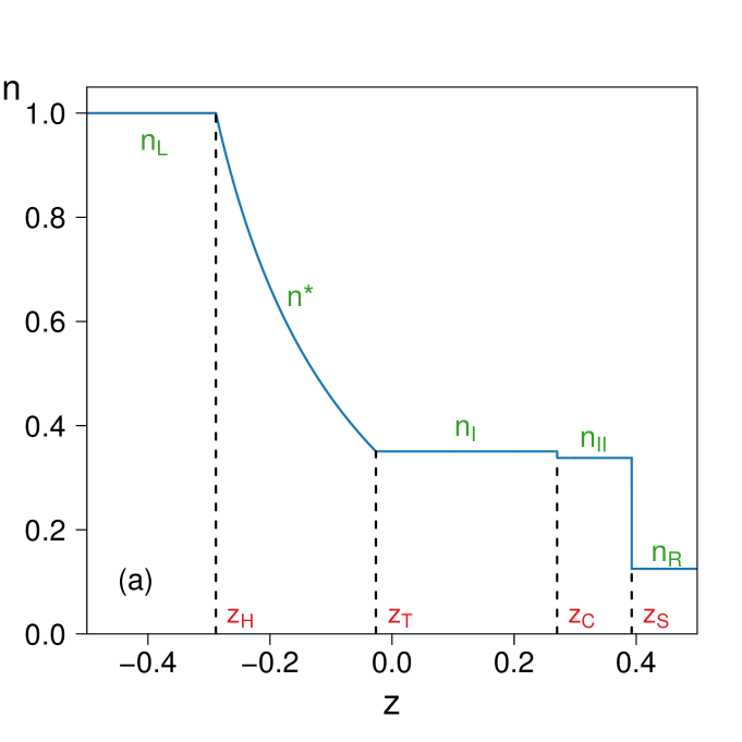
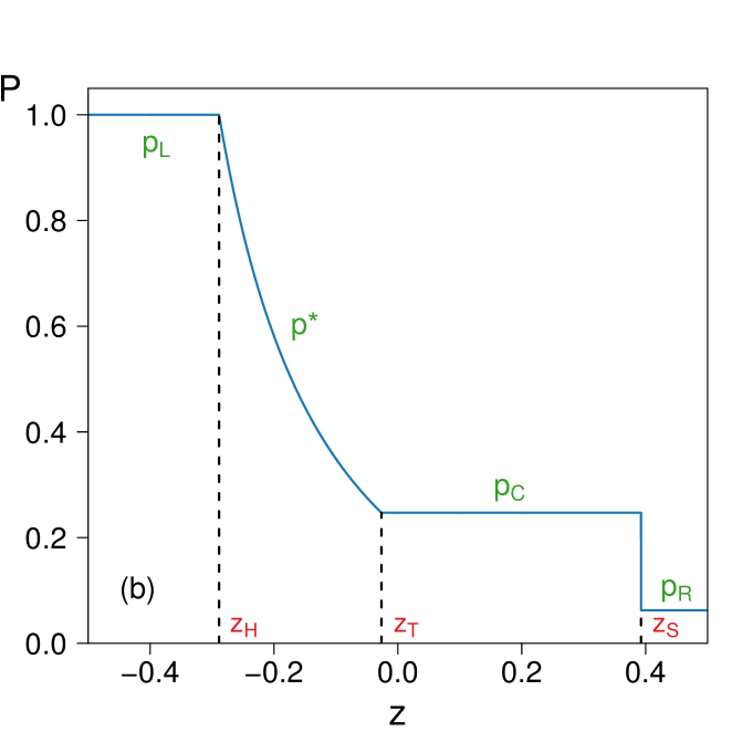
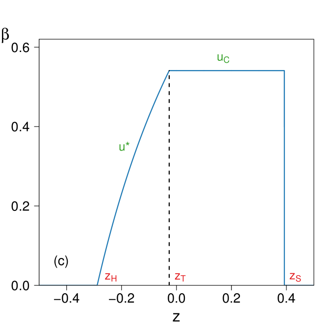
Figure 1: The flow structure in the inviscid limit of the Sod shock tube problem.

For the initial state in our simulations, we consider two chambers separated by a thin membrane. The two parts of the fluid are in different states such that the macroscopic fields describing the state of the fluid are discontinuous at the interface. Although the setup is very simple, the presence of large gradients make it a powerful test for numerical methods. We assume that, before the membrane is removed, the fluid constituents in the two domains are in local thermal equilibrium described by the following initial conditions:

$$(P,n,\beta)=\begin{cases}(P_{\text{\tiny L}},n_{\text{\tiny L}},\beta_{\text{\tiny L}}=0)&\text{if}\ \ z<0,\\ (P_{\text{\tiny R}},n_{\text{\tiny R}},\beta_{\text{\tiny R}}=0)&\text{if}\ \ z>0.\end{cases}$$ (133)

In the following, we take the reference pressure $\widetilde{P}_{\rm ref}$, temperature $\widetilde{T}_{\rm ref}$ and density $\widetilde{n}_{\rm ref}$ to be those of the left initial state, i.e.,

$$\widetilde{T}_{\text{\tiny ref}}=\widetilde{T}_{\text{\tiny L}},\qquad\widetilde{P}_{\text{\tiny ref}}=\widetilde{P}_{\text{\tiny L}},\qquad\widetilde{n}_{\text{\tiny ref}}=\widetilde{n}_{\text{\tiny L}}.$$ (134)

In the above, we employed the convention that dimensional quantities are denoted using a tilde $\widetilde{\phantom{T}}$. The above choice implies that $P_{\text{\tiny L}}=n_{\text{\tiny L}}=T_{\text{\tiny L}}=1$, which is the convention that we will use throughout this section. Furthermore, the reference length $\widetilde{L}_{\text{\tiny ref}}$ is chosen to be equal to the domain length, while the reference velocity $\widetilde{v}_{\text{\tiny ref}}=\widetilde{c}$ is chosen to be the speed of light. This implies the following definition for the reference time:

$$\widetilde{t}_{\text{\tiny ref}}=\frac{\widetilde{L}_{\text{\tiny ref}}}{\widetilde{c}}.$$ (135)

In the ideal (inviscid) case, as the system evolves in time, we see the formation of a rarefaction wave (R) moving to the left, as well as a contact discontinuity (C) and shock wave (S) moving to the right. As shown in Fig. 1, these features divide the flow into 5 regions: regions L and R represent the initial unperturbed states to the left of the rarefaction wave and to the right of the shock wave, regions I and II form the central plateau C to the left and right of the contact discontinuity, and the * region consists of the interval between the head and tail of the rarefaction wave. The region to which a particular macroscopic field refers will be indicated via a subscript (e.g., $P_{*}$ refers to the pressure in the rarefaction wave). A complete solution of the Riemann problem in the inviscid regime is represented by finding the values of the fields in the intermediate regions I, II, and * in terms of the initial conditions from the external unperturbed regions L and R. For completeness, we present in detail the procedure for obtaining such a solution in Sec. IV.2.

As the viscosity is increased, dissipation causes the interfaces between the above mentioned regions to become smooth, while in the ballistic regime, the fluid constituents stream freely, such that the above regions become indistinguishable. In the viscous regime, we follow Ref. Bouras et al. (2009a) and characterize the degree of rarefaction using the ratio $(\overline{\eta/s})$ (assumed to be constant) between the shear viscosity $\eta$ and the entropy density $s$, expressed in Planck units. The connection between $(\overline{\eta/s})$ and the nondimensionalized Anderson-Witting relaxation time $\tau_{\text{\tiny A-W}}$ employed in this paper can be established as follows.

The nondimensional relaxation time $\tau_{\text{\tiny A-W}}=\widetilde{\tau}_{\text{\tiny A-W}}/\widetilde{t}_{\text{\tiny ref}}$ can be related to the ratio $\widetilde{\eta}/\widetilde{s}$ starting from Cercignani and Kremer (2002):

$$\frac{\widetilde{\eta}}{\widetilde{s}}=\frac{4\widetilde{\tau}_{\text{\tiny A-W}}\widetilde{T}}{5(4-\ln\lambda)},$$ (136)

where the fugacity $\lambda$ is defined as Cercignani and Kremer (2002):

$$\lambda=\frac{\widetilde{n}\pi^{2}}{g_{s}}\left(\frac{\widetilde{\hbar}\widetilde{c}}{\widetilde{k}_{B}\widetilde{T}}\right)^{3}.$$ (137)

In the context of quark-gluon plasma systems, $g_{s}=16$ is the number of degrees of freedom for gluons. It is convenient to express $\lambda=\overline{\lambda}\lambda_{\text{\tiny ref}}$ using the relative fugacity $\overline{\lambda}$ (35), in terms of the fugacity $\lambda_{\text{\tiny ref}}=\lambda_{\text{\tiny L}}$ in the left side of the channel:

$$\overline{\lambda}=\frac{n}{T^{3}},\qquad\lambda_{\text{\tiny ref}}=\frac{\widetilde{n}_{\text{\tiny ref}}\pi^{2}}{g_{s}}\left(\frac{\widetilde{\hbar}\widetilde{c}}{\widetilde{k}_{B}\widetilde{T}_{\text{\tiny ref}}}\right)^{3}.$$ (138)

With the above notation, $\tau_{\text{\tiny A-W}}$ can be obtained from Eq. (136) as:

$$\tau_{\text{\tiny A-W}}=\frac{\eta}{s}\frac{5}{4T}[4-\ln(\overline{\lambda}\lambda_{\text{\tiny ref}})],$$ (139)

where $\eta/s$ is:

$$\frac{\eta}{s}=\frac{\widetilde{\eta}}{\widetilde{s}}\frac{\widetilde{c}}{\widetilde{T}_{\text{\tiny ref}}\widetilde{L}_{\text{\tiny ref}}}.$$ (140)

The connection between $(\overline{\eta/s})$ and the ratio $\eta/s$ obtained by applying the non-dimensionalization procedure discussed in this subsection can be established as follows:

$$(\overline{\eta/s})\equiv\frac{\widetilde{k}_{B}}{\widetilde{\hbar}}\left(\frac{\widetilde{\eta}}{\widetilde{s}}\right)=\frac{\widetilde{k}_{B}\widetilde{T}_{\text{\tiny ref}}\widetilde{L}_{\text{\tiny ref}}}{\widetilde{\hbar}\widetilde{c}}\left(\frac{\eta}{s}\right).$$ (141)

The above procedure gives the following expression for the non-dimensional relaxation time $\tau_{\text{\tiny A-W}}$:

$$\tau_{\text{\tiny A-W}}= \frac{\tau_{\text{\tiny A-W};0}}{T}\left[1-\frac{1}{4}\ln(\overline{\lambda}\lambda_{\text{\tiny ref}})\right],$$

$$\tau_{\text{\tiny A-W};0}= 5\frac{\widetilde{\hbar}\widetilde{c}(\overline{\eta/s})}{\widetilde{k}_{B}\widetilde{T}_{\text{\tiny ref}}\widetilde{L}_{\text{\tiny ref}}}.$$ (142)

As discussed at the beginning of this subsection, at $t=0$, the system is initialized using

$$f(z,t=0)=\begin{cases}f^{\text{\tiny(eq)}}_{\text{\tiny L}},&z<0,\\ f^{\text{\tiny(eq)}}_{\text{\tiny R}},&z>0,\end{cases}$$ (143)

where

$$f^{\text{\tiny(eq)}}_{\text{\tiny L}}=\frac{n_{\text{\tiny L}}}{8\pi T_{\text{\tiny L}}^{3}}e^{-p/T_{\text{\tiny L}}},\qquad f^{\text{\tiny(eq)}}_{\text{\tiny R}}=\frac{n_{\text{\tiny R}}}{8\pi T_{\text{\tiny R}}^{3}}e^{-p/T_{\text{\tiny R}}}.$$ (144)

In order to employ the numerical scheme described in Sec. III.6, boundary conditions must be employed to the left and right of the fluid domain. Since the WENO5 scheme requires information from three nodes in the upstream direction, three ghost nodes are required on both sides of the fluid domain. According to the discussion in Sec. III.6, the nodes to the left of the fluid domain have labels $s=0,\ -1$ and $-2$, while the nodes to the right are given by $s=Z+1$, $Z+2$, and $Z+3$. In this paper, we follow Ref. Gan et al. (2011) and set:

$$f_{n;0;jk}=f_{n;-1;jk}=f_{n;-2;jk}= f^{\text{\tiny(eq)}}_{\text{\tiny L};jk},$$

$$f_{n;Z+1;jk}=f_{n;Z+2;jk}=f_{n;Z+3;jk}= f^{\text{\tiny(eq)}}_{\text{\tiny R};jk}.$$ (145)

IV.2 Inviscid regime

The analytic solution for the Sod shock tube problem is well known Rezzolla and Zanotti (2013). Since the solution is usually not particularized for the case of massless particles considered in this paper, we review the derivation of the analytic solution for this case in Sec. IV.2.1. Our simulation results for the macroscopic profiles are presented in Sec. IV.2.2. In order to assess the capabilities of our models to recover dissipative effects, we present in Sec. IV.2.3 an analysis of the nonequilibrium quantities (heat flux and shear stress) induced near the flow discontinuities.

IV.2.1 Analytic profiles

In the case of the Riemann problem with the initial conditions (133), the density profile of the flow at a finite time contains three features: a rarefaction wave (R) traveling to the left and a shock wave (S) and contact discontinuity (C) traveling to the right. The rarefaction wave is a simple wave. This means that the flow is isentropic and has a number of Riemann invariants, properties which can be exploited to obtain the values of the thermodynamic fields inside the wave Rezzolla and Zanotti (2013). In the case of shock-waves either one or several of the fields present discontinuities. The macroscopic conservation equations then induce a number of junction conditions (the Rankine-Hugoniot junction conditions) involving the density, pressure, and velocity of the fluid on the two sides of the discontinuity.

Rarefaction wave.

In order to find relations that determine the fields inside the rarefaction wave, we start from the macroscopic conservation equations Cercignani and Kremer (2002):

$$Dn= -n\,\partial_{\mu}u^{\mu},$$

$$Du^{\alpha}= -\frac{1}{4P}\Delta^{\alpha\mu}\partial_{\mu}P,$$

$$DP= -\frac{4P}{3}\partial_{\mu}u^{\mu},$$ (146)

where $D=u^{\alpha}\partial_{\alpha}=\gamma(\partial_{t}+\beta\partial_{z})$ and $\Delta^{\alpha\beta}=\eta^{\alpha\beta}+u^{\alpha}u^{\beta}$. The rarefaction wave, as any simple wave, is self-similar. This means that the fields depend on space and time only through the self-similarity variable $\zeta=\frac{z}{t}$, such that Eq. (146) becomes:

$$(\beta-\zeta)\frac{dn}{d\zeta}\ = -n\gamma^{2}(1-\beta\zeta)\frac{d\beta}{d\zeta},$$ (147a)

$$(\beta-\zeta)\frac{d\beta}{d\zeta}= -\frac{1}{4P\gamma^{2}}(1-\beta\zeta)\frac{dP}{d\zeta},$$ (147b)

$$(\beta-\zeta)\frac{dP}{d\zeta}\ = -\frac{4P}{3}\gamma^{2}(1-\beta\zeta)\frac{d\beta}{d\zeta}.$$ (147c)

Using Eq. (147c) to eliminate the pressure in Eq. (147b) gives the following constraint for $\zeta$:

$$\zeta=\frac{\beta\mp c_{s}}{1\mp c_{s}\beta},$$ (148)

where $c_{s}=1/\sqrt{3}$ is the speed of sound for an ultrarelativistic fluid. The lower sign refers to the case when the rarefaction wave moves to the right and is therefore irrelevant for the present case. Plugging relation (148) back into Eqs. (147a) and (147c) gives:

$$\frac{1}{n\sqrt{3}}\frac{dn}{d\zeta}+\gamma^{2}\frac{d\beta}{d\zeta}= 0,$$

$$\frac{\sqrt{3}}{4P}\frac{dP}{d\zeta}+\gamma^{2}\frac{d\beta}{d\zeta}= 0.$$ (149)

Integrating these relations and with a bit of rearrangement, the expressions for the Riemann invariants can be obtained:

$$n\left(\frac{1+\beta}{1-\beta}\right)^{\frac{\sqrt{3}}{2}}=\text{const},\qquad P\left(\frac{1+\beta}{1-\beta}\right)^{\frac{2}{\sqrt{3}}}=\text{const}.$$ (150)

The Riemann invariants are conserved along the rarefaction wave,thus allowing the quantities in this region (denoted using a star $*$) to be expressed as functions of the parameters in the unperturbed left state ($n_{\text{\tiny L}},P_{\text{\tiny L}},\beta_{\text{\tiny L}}=0$):

$$\beta_{*}= \frac{c_{s}+\zeta}{1+c_{s}\zeta},$$ (151a)

$$P_{*}= P_{\text{\tiny L}}\left[\frac{(1-c_{s})(1-\zeta)}{(1+c_{s})(1+\zeta)}\right]^{2/\sqrt{3}},$$ (151b)

$$n_{*}= n_{\text{\tiny L}}\left[\frac{(1-c_{s})(1-\zeta)}{(1+c_{s})(1+\zeta)}\right]^{\sqrt{3}/2}.$$ (151c)

It can be seen that throughout the rarefaction wave, the relative fugacity (35) remains equal to the relative fugacity in the left state:

$$\overline{\lambda}_{*}=\frac{n_{*}^{4}}{P_{*}^{3}}=\frac{n_{\text{\tiny L}}^{4}}{P_{\text{\tiny L}}^{3}}=\overline{\lambda}_{\text{\tiny L}}.$$ (152)

Once the similarity variable $\zeta_{T}$ of the tail of the rarefaction wave is known, the values of $n_{\text{\tiny I}}$, $P_{\text{\tiny C}}$, and $\beta_{\text{\tiny C}}$ can be found. The problem is resolved by finding the velocity on the central plateau (from the conditions at the shock front) and matching with Eq. (148).

Shock wave.

In the hydrodynamic description, the shockwaves represent discontinuities in the values of the macroscopic fields of the fluid. The values of these quantities to the left and right of the shockwave are given by the Rankine-Hugoniot junction conditions Rezzolla and Zanotti (2013):

$$n_{\text{\tiny II}}\,\gamma_{\text{\tiny C,{S}}}\,\beta_{\text{\tiny C,{S}}}= n_{\text{\tiny R}}\,\gamma_{\text{\tiny R,{S}}}\,\beta_{\text{\tiny R,{S}}},$$ (153a)

$$P_{\text{\tiny C}}\gamma_{\text{\tiny C,{S}}}^{2}\left(1+3\,\beta_{\text{\tiny C,{S}}}^{2}\right)= P_{\text{\tiny R}}\gamma_{\text{\tiny R,{S}}}^{2}\,\left(1+3\,\beta_{\text{\tiny R,{S}}}^{2}\right),$$ (153b)

$$P_{\text{\tiny C}}\gamma_{\text{\tiny C,{S}}}^{2}\beta_{\text{\tiny C,{S}}}= P_{\text{\tiny R}}\gamma_{\text{\tiny R,{S}}}^{2}\beta_{\text{\tiny R,{S}}},$$ (153c)

where the subscript $s$ indicates that the velocities $\beta_{\text{\tiny C,{S}}}$ and $\beta_{\text{\tiny R,{S}}}$ are evaluated in the rest frame of the shock front. Manipulating Eq. (153), the velocities of the fluid on the two sides of the shock can be obtained:

$$\beta_{\text{\tiny C,{S}}}=-\sqrt{\frac{P_{\text{\tiny C}}+3P_{\text{\tiny R}}}{3(P_{\text{\tiny R}}+3P_{\text{\tiny C}})}},\qquad\beta_{\text{\tiny R,{S}}}=-\sqrt{\frac{P_{\text{\tiny R}}+3P_{\text{\tiny C}}}{3(P_{\text{\tiny C}}+3P_{\text{\tiny R}})}}.$$ (154)

The velocities of the shock front and on the central plateau with respect to the Eulerian frame in which the unperturbed fluid is at rest can be obtained using the relativistic law of velocity composition:

$$\beta_{\text{\tiny shock}}=\sqrt{\frac{P_{\text{\tiny R}}+3P_{\text{\tiny C}}}{3(P_{\text{\tiny C}}+3P_{\text{\tiny R}})}},{}$$

$$\beta_{\text{\tiny C}}=\frac{\beta_{\text{\tiny C,{S}}}-\beta_{\text{\tiny R,{S}}}}{1-\beta_{\text{\tiny C,{S}}}\beta_{\text{\tiny R,{S}}}}=\sqrt{\frac{3(P_{\text{\tiny C}}-P_{\text{\tiny R}})^{2}}{(P_{\text{\tiny C}}+3P_{\text{\tiny{R}}})(3P_{\text{\tiny C}}+P_{\text{\tiny{R}}})}}.$$ (155)

From the first junction condition (153), the density in the left side of the shock $n_{\text{\tiny II}}$ can be obtained as:

$$n_{\text{\tiny II}}=n_{\text{\tiny R}}\frac{\gamma_{\text{\tiny R,{S}}}\,\beta_{\text{\tiny R,{S}}}}{\gamma_{\text{\tiny C,{S}}}\,\beta_{\text{\tiny C,{S}}}}=n_{R}\sqrt{\frac{P_{C}(P_{R}+3P_{C})}{P_{R}(P_{C}+3P_{R})}}.$$ (156)

Contact discontinuity and central plateau.

The contact discontinuity is a particular kind of shockwave where there is no mass transport through the discontinuity surface with the pressure and velocity of the fluid being constant throughout, such that $\beta_{\text{\tiny I}}=\beta_{\text{\tiny II}}\equiv\beta_{\text{\tiny C}}$, $P_{\text{\tiny I}}=P_{\text{\tiny II}}\equiv P_{\text{\tiny C}}$, and $n_{\text{\tiny I}}\neq n_{\text{\tiny II}}$.

The last parameter needed to find the complete solution of the Sod problem is the pressure on the plateau. This can be found by requiring that Eqs. (155), (151b), and (148) are simultaneously satisfied. This yields the following expression for the coordinate of the rarefaction tail $\zeta_{\text{\tiny T}}$:

$$\zeta_{\text{\tiny T}}=\frac{\sqrt{3}-1-(\sqrt{3}+1)(P_{\text{\tiny C}}/P_{\text{\tiny L}})^{\sqrt{3}/2}}{\sqrt{3}-1+(\sqrt{3}+1)(P_{\text{\tiny C}}/P_{\text{\tiny L}})^{\sqrt{3}/2}}.$$ (157)

The pressure on the central plateau $P_{\text{\tiny C}}$ can be found as a root of the equation

$$\frac{(P_{\text{\tiny L}}/P_{\text{\tiny C}})^{\sqrt{3}/2}-1}{(P_{\text{\tiny L}}/P_{\text{\tiny C}})^{\sqrt{3}/2}+1}-\sqrt{\frac{3(P_{\text{\tiny C}}-P_{\text{\tiny R}})^{2}}{(P_{\text{\tiny C}}+3P_{\text{\tiny R}})(3P_{\text{\tiny C}}+P_{\text{\tiny R}})}}=0.$$ (158)

The density $n_{\text{\tiny I}}$ between the rarefaction tail and the contact discontinuity can be found using Eq. (151c) with $\zeta=\zeta_{\text{\tiny T}}$:

$$n_{\text{\tiny I}}=n_{\text{\tiny L}}\left(\frac{P_{\text{\tiny C}}}{P_{\text{\tiny L}}}\right)^{3/4}.$$ (159)

Full solution.

In order to obtain the full solution of the Sod shock tube problem, the following steps can be taken. First, the pressure on the central plateau $P_{\text{\tiny C}}$ can be found as a root of Eq. (158). Then, the shock front velocity $\beta_{\text{\tiny shock}}$, central plateau velocity $\beta_{\text{\tiny C}}$, and rarefaction tail similarity coordinate $\zeta_{T}$ can be found using Eqs. (155) and (157). The densities $n_{\text{\tiny I}}$ and $n_{\text{\tiny II}}$ to the left and right of the contact discontinuity can be found using Eqs. (159) and (156), respectively. The structure of the full solution is represented in Fig. 1 and has the following mathematical formulation:

$$\beta(z,t)=\begin{cases}\beta_{\text{\tiny L}},&z<z_{\text{\tiny H}},\\ \beta_{*},&z_{\text{\tiny H}}<z<z_{\text{\tiny T}},\\ \beta_{\text{\tiny C}},&z_{\text{\tiny T}}<z<z_{\text{\tiny S}},\\ \beta_{\text{\tiny R}},&z>z_{\text{\tiny S}},\end{cases}{}$$

$$P(z,t)=\begin{cases}P_{\text{\tiny L}},&z<z_{\text{\tiny H}},\\ P_{*},&z_{\text{\tiny H}}<z<z_{\text{\tiny T}},\\ P_{\text{\tiny C}},&z_{\text{\tiny T}}<z<z_{\text{\tiny S}},\\ P_{\text{\tiny R}},&z>z_{\text{\tiny S}},\end{cases},$$

$$n(z,t)=\begin{cases}n_{\text{\tiny L}},&z<z_{\text{\tiny H}},\\ n_{*},&z_{\text{\tiny H}}<z<z_{\text{\tiny T}},\\ n_{\text{\tiny I}},&z_{\text{\tiny T}}<z<z_{\text{\tiny C}},\\ n_{\text{\tiny II}},&z_{\text{\tiny C}}<z<z_{\text{\tiny S}},\\ n_{\text{\tiny R}},&z>z_{\text{\tiny S}}.\end{cases}$$ (160)

In the above, $z_{\text{\tiny H}}$ ($z_{\text{\tiny T}}$), $z_{\text{\tiny C}}$ and $z_{\text{\tiny S}}$ represent the locations of the head (tail) of the rarefaction wave, of the contact discontinuity and of the shock front, respectively, being given by

$$z_{\text{\tiny H}}= -c_{s}t,\qquad z_{\text{\tiny T}}=\left(\frac{\beta_{\text{\tiny C}}-c_{s}}{1-\beta_{\text{\tiny C}}c_{s}}\right)t,\qquad$$ (161)

$$z_{\text{\tiny C}}= \,\beta_{\text{\tiny C}}t,\qquad\quad z_{\text{\tiny S}}=\beta_{\text{\tiny shock}}t,$$ (162)

where $c_{s}=1/\sqrt{3}$ is the sound speed and $\beta_{\text{\tiny C}}$ and $\beta_{\text{\tiny shock}}$ are given in Eq. (155).

IV.2.2 Macroscopic profiles

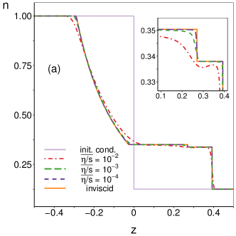
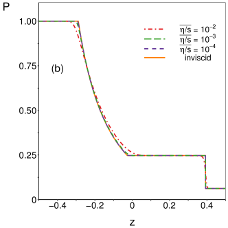
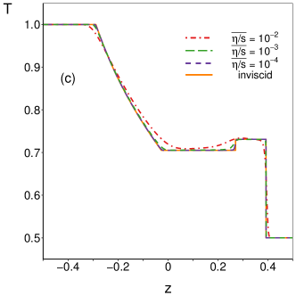
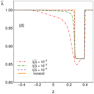
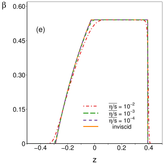
Figure 2: Density (a), pressure (b), temperature (c), fugacity (d) and velocity (e) profiles for decreasing values of the ratio $(\overline{\eta/s})$, compared with the analytical results for the inviscid limit, presented in Sec. IV.2.1. The quadrature order is $Q_{\xi}=6$, the number of points is $Z=10\,000$, the time step was set to $5\times 10^{-6}$ and the snapshot corresponds to $t=0.5$ (i.e., $100\,000$ iterations were performed). The initial conditions are $(n_{\text{\tiny L}},T_{\text{\tiny L}},P_{\text{\tiny L}})=(1,1,1)$ and $(n_{\text{\tiny R}},T_{\text{\tiny R}},P_{\text{\tiny R}})=(0.125,0.5,0.0625)$.

Let us now specialize the solution obtained in Sec. IV.2.1 to the case considered in Refs. Bouras et al. (2010, 2009b); Hupp et al. (2011); Mohseni et al. (2013), where

$$\widetilde{k}_{B}\widetilde{T}_{\text{\tiny ref}}=0.4\ {\rm GeV},\qquad\widetilde{P}_{\text{\tiny ref}}=5.43\ {\rm GeV}/{\rm fm}^{3},{}$$

$$\widetilde{n}_{\text{\tiny ref}}=13.57\ {\rm fm}^{-3},$$ (163)

while the reference length is $\widetilde{L}_{\text{\tiny ref}}=6.4\ {\rm fm}$. With the above quantities, $\lambda_{\text{\tiny ref}}\simeq 1$ and

$$\tau_{\text{\tiny A-W}}= \frac{\tau_{\text{\tiny A-W};0}}{T}\left(1-\frac{\ln\overline{\lambda}}{4}\right),$$

$$\tau_{\text{\tiny A-W};0}\simeq 0.3854(\overline{\eta/s}).$$ (164)

The reference quantities given in Eq. (163) refer to the initial state in the left half of the channel. In the right half, the following values are used:

$$\widetilde{k}_{B}\widetilde{T}_{\text{\tiny R}}=0.2\ {\rm GeV},\qquad\widetilde{P}_{\text{\tiny R}}=0.33\ {\rm GeV}/{\rm fm}^{3},{}$$

$$\widetilde{n}_{\text{\tiny R}}=1.66\ {\rm fm}^{-3},$$ (165)

which correspond to:

$$T_{\text{\tiny R}}=0.5,\qquad P_{\text{\tiny R}}=0.0625,\qquad n_{\text{\tiny R}}=0.125.$$ (166)

With the above values, the relative fugacity (35) at initial time is constant throughout the channel:

$$\overline{\lambda}_{\text{\tiny L}}=\overline{\lambda}_{\text{\tiny R}}=1.$$ (167)

The relaxation times in the two halves of the channel are:

$$\tau_{\text{\tiny A-W};\text{\tiny L}}\simeq 0.3854(\overline{\eta/s}),\qquad\tau_{\text{\tiny A-W};\text{\tiny R}}\simeq 0.7708(\overline{\eta/s}).$$ (168)

Applying the analysis in Sec. IV.2.1, the following numerical values are obtained:

$$\beta_{\text{\tiny shock}}\simeq 0.785,\qquad\beta_{\text{\tiny C}}\simeq 0.541,{}$$

$$P_{\text{\tiny C}}\simeq 0.247,\qquad n_{\text{\tiny I}}\simeq 0.350,\qquad n_{\text{\tiny II}}\simeq 0.338,$$ (169)

while the rarefaction head and tail are located at $z_{\text{\tiny H}}=-t/\sqrt{3}\simeq-0.577t$ and $z_{T}=\zeta_{T}t\simeq-0.053t$. The contact discontinuity is located at $z_{\text{\tiny C}}=\beta_{\text{\tiny C}}t\simeq 0.541t$.

Figure 2 shows the profiles of $n$, $P$, $T$, and $\overline{\lambda}$ obtained from our simulations at various values of $(\overline{\eta/s})$. The convergence towards the analytical result can be clearly seen as $(\overline{\eta/s})\rightarrow 0$ (the inviscid limit). For these simulations, we used a grid of $Z=10\,000$ nodes and a time step of $\delta t=5\times 10^{-6}$. While the shock front in the particle number density profile is already well recovered at $(\overline{\eta/s})=10^{-3}$, at $(\overline{\eta/s})=10^{-4}$ it spans around four to six grid points, which is equivalent to $0.04$–$0.06\%$ of the size of the domain.

The orders of the quadratures are fixed at $Q_{\text{\tiny L}}=2$, $Q_{\varphi}=1$, and $Q_{\xi}=6$ for the radial, azimuthal and polar quadratures, while the expansion of $f^{\text{\tiny(eq)}}$ was truncated at $N_{\text{\tiny L}}=1$ and $N_{\Omega}=5$. We remind the reader that the values $Q_{\xi}=6$ and $N_{\Omega}=5$ are used here to validate a benchmark “reference profile,” while in Sec. IV.5, the capabilities of models with smaller values of $Q_{\xi}$ and $N_{\Omega}$ will be discussed.

If $(\overline{\eta/s})$ is decreased below $10^{-4}$ while keeping $\delta t$ and $\delta z$ fixed at the values used above, the macroscopic profiles start developing spurious oscillations. For the values of $(\overline{\eta/s})\geq 10^{-4}$, our simulations are stable, mainly due to the increased stability ensured by the combination of the fifth order WENO and third order Runge-Kutta schemes, employed for the implementation of the spatial and temporal derivatives, respectively.

IV.2.3 Non-equilibrium quantities and dissipative effects

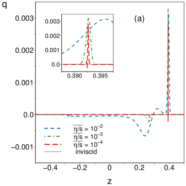
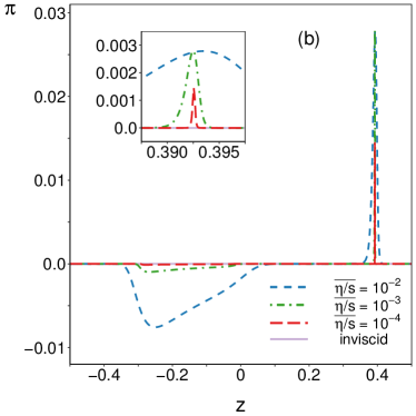
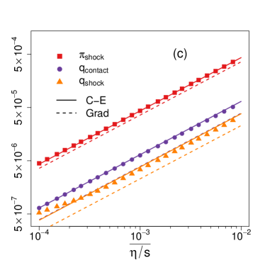
Figure 3: Profiles of $q$ (a) and $\Pi$ (b) for decreasing values of $(\overline{\eta/s})$. (c) The integrated values of $q$ and $\Pi$ over small vicinities around the contact discontinuity and the shock front are shown in absolute value as functions of $(\overline{\eta/s})$ in log-log scale (the integral of $\Pi$ around the contact discontinuity is not shown, since $\Pi$ vanishes in this region). The analytic results (175) and (176) are also represented for comparison, for values of the transport coefficients obtained with both the Chapman-Enskog (solid lines) and Grad (dashed lines) methods. The simulation parameters are presented in the caption of Fig. 2.

In Subsec. IV.2.1, we considered the flow of a perfect fluid. In theory, this corresponds to taking the limit of vanishing relaxation time in the Anderson-Witting Boltzmann equation (38). In our implementation of the Boltzmann equation, the relaxation time can never be decreased to $0$, such that the transport coefficients defined in Eqs. (36b), assumed to vanish in the inviscid limit presented above, will always be finite. According to Eqs. (34), the heat flux $q^{\mu}$ and pressure deviator $\Pi^{\mu\nu}$ can be obtained in the hydrodynamic regime (small values of $\tau_{\text{\tiny A-W}}$) by taking gradients of $T$, $P$ and $u^{\mu}$. In the inviscid limit, these quantities are discontinuous in the vicinity of the shock front and of the contact discontinuity (the pressure and velocity are discontinuous only at the shock front). Thus, it is natural to expect that their gradients will be sharply peaked in these regions.

As mentioned in Sec. II.5, $q^{\mu}$ and $\Pi^{\mu\nu}$ can be fully characterized by the scalar quantities $q$ (44) and $\Pi$ (46), which we represent in Fig. 3. It can be seen in plot (a) that $q$ presents a strong fluctuation around the contact discontinuity, while plot (b) demonstrates that $\Pi$ has nonvanishing values mostly around the rarefaction wave, peaking towards its head. Both $q$ and $\Pi$ exhibit a strong spike at the shock front, even when $(\overline{\eta/s})=10^{-4}$, induced via Eqs. (34) due to the strong gradients of the macroscopic fields. The width of this spike decreases as $(\overline{\eta/s})$ is decreased and the shock front becomes narrower.

In this subsection, we consider a quantitative analysis of these nonequilibrium effects by evaluating the integrated values of $q$ and $\Pi$ over the regions where they are non-negligible. The value of these integrals can be estimated analytically by considering the flow to be close to the inviscid limit, where the solution for the macroscopic profiles is given in Sec. IV.2.1.

Considering that the macroscopic fields depend only on the similarity variable $\zeta=z/t$, the action of the convective derivative $D=u^{\mu}\partial_{\mu}$ and of $\Delta^{\mu\nu}\partial_{\nu}=\eta^{\mu\nu}\partial_{\nu}+u^{\mu}D$ on an arbitrary function $f(\zeta)$ can be reduced to:

$$Df(\zeta)= \frac{\gamma}{t}(\beta-\zeta)\partial_{\zeta}f,$$ (170a)

$$\Delta^{\mu\nu}\partial_{\nu}f(\zeta)= \frac{\gamma^{2}}{t}\left(\delta^{\mu}{}_{z}+\beta\delta^{\mu}{}_{0}\right)(1-\beta\zeta)\partial_{\zeta}f.$$ (170b)

With the above formulas, Eqs. (34b) and (34c) can be used to find $q$ and $\Pi$ as:

$$q= \frac{\lambda_{\text{\tiny heat}}T}{4}\Delta^{z\nu}\partial_{\nu}\ln\overline{\lambda}=\frac{\lambda_{\text{\tiny heat}}T\gamma^{2}}{4t}(1-\beta\zeta)\partial_{\zeta}\ln\overline{\lambda},$$ (171a)

$$\Pi= -\frac{4\eta}{3}\partial_{\mu}u^{\mu}=-\frac{4\eta}{3t}(1-\beta\zeta)\partial_{\zeta}(\gamma\beta),$$ (171b)

where the definition (35) for the relative fugacity $\overline{\lambda}$ was employed.

Since, according to Eq. (152), $\overline{\lambda}$ is constant from the unperturbed region on the left up to the contact discontinuity, $q$ vanishes in this region. This is confirmed in Fig. 3(a). Similarly, $\Pi$ vanishes between the tail of the rarefaction and the shock front, since $\beta=\beta_{\text{\tiny C}}$ is constant in this region. Figure 3(b) confirms this prediction.

Close to the shock front, both $q$ and $\Pi$ can be put in the form:

$$f_{\text{\tiny disc}}=\frac{1}{t}g(\zeta)\partial_{\zeta}h(\zeta),$$ (172)

where both $g$ and $h$ may be discontinuous at $\zeta=\zeta_{d}$. Using the Heaviside step function, $g(\zeta)$ and $\partial_{\zeta}h(\zeta)$ can be written as:

$$g(\zeta)= \theta(\zeta-\zeta_{d})g_{>}+\theta(\zeta_{d}-\zeta)g_{<},$$ (173a)

$$\partial_{\zeta}h(\zeta)= \delta(\zeta-\zeta_{d})(h_{>}-h_{<}),$$ (173b)

where the subscript $>$ ($<$) denotes the value of the function $g(\zeta)$ or $h(\zeta)$ to the right (left) of the discontinuity. The integral of $f_{\text{\tiny disc}}$ over a small region $z_{d}\pm\delta z$ around the point $z_{d}=\zeta_{d}t$ is given by:

$$\lim_{\delta z\rightarrow 0}\int_{z_{d}-\delta z}^{z_{d}+\delta z}f_{\text{\tiny disc}}dz=\frac{1}{2}(g_{>}+g_{<})(h_{>}-h_{<}).$$ (174)

The value of the integrals of $q$ over the vicinity of the contact discontinuity and of the shock front can be estimated through

contact: $$\int_{z_{\text{\tiny C}}-\delta z}^{z_{\text{\tiny C}}+\delta z}q\,dz=\frac{1}{8}(\lambda_{\text{\tiny heat},\text{\tiny I}}T_{\text{\tiny I}}+\lambda_{\text{\tiny heat},\text{\tiny II}}T_{\text{\tiny II}})\ln\frac{\overline{\lambda}_{\text{\tiny II}}}{\overline{\lambda}_{\text{\tiny I}}},$$ (175a)

shock: $$\int_{z_{\text{\tiny S}}-\delta z}^{z_{\text{\tiny S}}+\delta z}q\,dz=\frac{1}{8}\left[\lambda_{\text{\tiny heat},R}T_{R}\right.$$

$$\hskip 20.0pt\left.+\lambda_{\text{\tiny heat},\text{\tiny II}}T_{\text{\tiny II}}\gamma_{\text{\tiny C}}^{2}(1-\beta_{\text{\tiny C}}\beta_{\text{\tiny shock}})\right]\ln\frac{\overline{\lambda}_{\text{\tiny R}}}{\overline{\lambda}_{\text{\tiny II}}}.$$ (175b)

Similar expressions can be found for the integrals of $\Pi$:

contact: $$\int_{z_{\text{\tiny C}}-\delta z}^{z_{\text{\tiny C}}+\delta z}\Pi\,dz=0,$$ (176a)

shock: $$\int_{z_{\text{\tiny S}}-\delta z}^{z_{\text{\tiny S}}+\delta z}\Pi\,dz=\frac{2v_{\text{\tiny C}}\gamma_{\text{\tiny C}}}{3}\left[\eta_{R}+\eta_{\text{\tiny II}}(1-v_{\text{\tiny C}}v_{\text{\tiny S}})\right].$$ (176b)

In Fig. 3(c), the numerical estimate of the integrals calculated in Eqs. (175) and (176) are compared with the above analytic results when the transport coefficients are obtained using either the Grad moment method (36a) or the Chapman-Enskog method (36b). The agreement between the numerical data and the analytic prediction when the Chapman-Enskog values of the transport coefficients are used is remarkably good, even when $(\overline{\eta/s})\simeq 5\times 10^{-3}$. This result confirms the analyses of Refs. Bhalerao et al. (2014); Ryblewski (2015); Florkowski et al. (2015b); Gabbana et al. (2017b); Ambrus (2018), where further evidence was found supporting the validity of the Chapman-Enskog (as opposed to the Grad method) expressions for the transport coefficients, even when large gradients are present.

IV.3 Ballistic regime

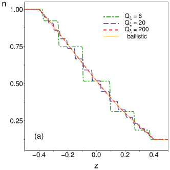
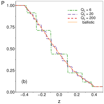
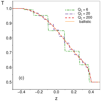
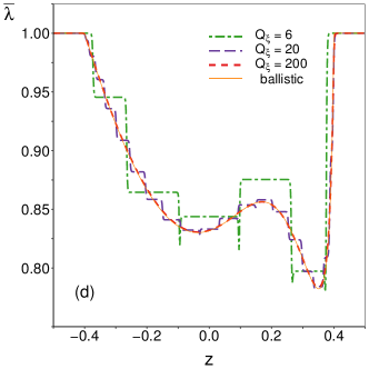
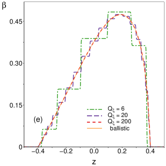
Figure 4: Profiles of the density (a), relative fugacity (b), pressure (c), temperature (d), and velocity (e), for different orders of the polar quadrature. The profiles corresponding to $Q_{\xi}=200$ are overlapped with the analytic solutions given in Sec. IV.3.1. The profiles represent snapshots at $t=0.4$, obtained using a number of $Z=1000$ nodes with a time step $\delta t=5\times 10^{-4}$. The initial state is described in the caption of Fig. 2.

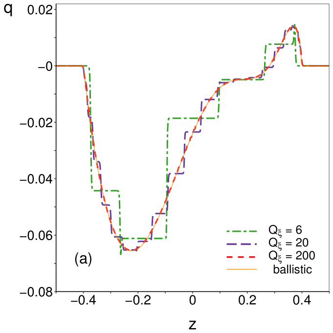
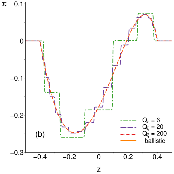
Figure 5: Ballistic regime profiles of the heatflux (a) and pressure deviator (b), for different orders of the polar quadrature. The simulation parameters are described in the caption of Fig.4.

In the ballistic case, the collision term vanishes and the Boltzmann equation (38) can be solved analytically (see, e.g., Refs. Greiner and Rischke (1996) and Guo et al. (2015) for the analytic treatment of the ballistic regime of the sphericallysymmetric relativistic and 1D nonrelativistic cases of the Riemann problem). For completeness, we present the free-streaming solution of the relativistic Sod shock tube problem in Sec. IV.3.1. Our numerical results are discussed in Sec. IV.3.2.

IV.3.1 Analytic solution

The collisionless version of the Boltzmann equation (38) reduces to:

$$\left(\partial_{t}+\xi\partial_{z}\right)f=0.$$ (177)

At initial time, the flow is in thermal equilibrium characterized by the macroscopic fields given in Eq. (133), such that

$$f(z,\xi,t=0)=\theta(-z)f^{\text{\tiny(eq)}}_{\text{\tiny L}}+\theta(z)f^{\text{\tiny(eq)}}_{\text{\tiny R}},$$ (178)

where

$$f^{\text{\tiny(eq)}}_{\text{\tiny L}/\text{\tiny R}}=\frac{n_{\text{\tiny L}/\text{\tiny R}}}{8\pi T^{3}_{\text{\tiny L}/\text{\tiny R}}}\exp\left(-\frac{p}{T_{\text{\tiny L}/\text{\tiny R}}}\right).$$ (179)

Equation (177) is automatically satisfied if $f\equiv f(z-\xi t)$, which can be combined with the initial condition (178) to yield:

$$f(\zeta,\xi)=\theta(\xi-\zeta)f^{\text{\tiny(eq)}}_{\text{\tiny L}}+\theta(\zeta-\xi)f^{\text{\tiny(eq)}}_{\text{\tiny R}},$$ (180)

where $\zeta=z/t$ and $t>0$ was assumed. Noting that, due to causality, the regions $\zeta>1$ and $\zeta<-1$ remain unperturbed, Eq. (180) can be put in the form

$$f(\zeta,\xi)=\begin{cases}f^{\text{\tiny(eq)}}_{\text{\tiny L}},&\zeta<-1,\\ \theta(\xi-\zeta)f^{\text{\tiny(eq)}}_{\text{\tiny L}}+\theta(\zeta-\xi)f^{\text{\tiny(eq)}}_{\text{\tiny R}},&|\zeta|<1,\\ f^{\text{\tiny(eq)}}_{\text{\tiny R}},&\zeta>1.\end{cases}$$ (181)

In the two external regions $|\zeta|>1$, the macroscopic fields are always at their initial equilibrium values. In the intermediate region, $N^{\mu}$ and $T^{\mu\nu}$ can be obtained through (23). Specifically, the nonvanishing components of $N^{\mu}$ are given by:

$$N^{0}(\zeta)= \left(\frac{n_{\text{\tiny L}}+n_{\text{\tiny R}}}{2}\right)-\left(\frac{n_{\text{\tiny L}}-n_{\text{\tiny R}}}{2}\right)\zeta,{}$$

$$N^{z}(\zeta)= \left(\frac{n_{\text{\tiny L}}-n_{\text{\tiny R}}}{4}\right)\left(1-\zeta^{2}\right),$$ (182)

while $N^{x}(t,z)=\ N^{y}(t,z)=0$, as expected from Eq. (40). Furthermore, the nonvanshing components of $T^{\mu\nu}$ are:

$$T^{00}= \frac{3}{2}(P_{\text{\tiny L}}+P_{\text{\tiny R}})-\frac{3}{2}(P_{\text{\tiny L}}-P_{\text{\tiny R}})\zeta,{}$$

$$T^{0z}= \frac{3}{4}(P_{\text{\tiny L}}-P_{\text{\tiny R}})\left(1-\zeta^{2}\right),{}$$

$$T^{zz}= \frac{1}{2}\left(P_{\text{\tiny L}}+P_{\text{\tiny R}}\right)-\frac{1}{2}\left(P_{\text{\tiny L}}-P_{\text{\tiny R}}\right)\zeta^{3},$$ (183)

while $T^{xx}=T^{yy}=\frac{1}{2}(T^{00}-T^{zz})$. The energy density $E$, macroscopic velocity $u^{\mu}$, heat flux $q$, and shear pressure $\Pi$ can be computed using Eqs. (42)–(47). Because their analytic expressions are cumbersome, we omit them here and mention that the profiles of these quantities can be represented in a straightforward manner using the above solution.

For completeness, we also include an analysis of the Eckart frame, in which the macroscopic velocity $u^{\mu}_{e}=\gamma_{e}(1,0,0,\beta_{e})^{T}$ is defined as the unit vector which is parallel to the particle four-flow $N^{\mu}$:

$$N^{\mu}=n_{e}u^{\mu}_{e},$$ (184)

While in the unperturbed regions, the macroscopic fields computed with respect to the Eckart and Landau frames coincide, in the perturbed regions they are generally different. The Eckart frame particle number density $n_{e}=-u^{\mu}_{e}N_{\mu}$ and velocity $\beta_{e}=u^{z}_{e}/u^{t}_{e}$ are given by:

$$n_{e}= \left[\left(\frac{1+\zeta}{2}n_{\text{\tiny R}}+\frac{1-\zeta}{2}n_{\text{\tiny L}}\right)^{2}\right.$$

$$\left.-\left(\frac{n_{\text{\tiny L}}-n_{\text{\tiny R}}}{2}\right)^{2}\left(\frac{1-\zeta^{2}}{2}\right)^{2}\right]^{1/2},$$ (185)

$$\beta_{e}= \frac{1}{2}\frac{(n_{\text{\tiny L}}-n_{\text{\tiny R}})\left(1-\zeta^{2}\right)}{\left(n_{\text{\tiny L}}+n_{\text{\tiny R}}\right)-\left(n_{\text{\tiny L}}-n_{\text{\tiny R}}\right)\zeta}.$$ (186)

The other macroscopic quantities (energy, pressure, shear stress, and heat flux) can be obtained from Eqs. (183), as follows:

$$E_{e}=u_{e}^{\mu}u_{e}^{\nu}T_{\mu\nu},\quad q_{e}^{\mu}=-\Delta^{\mu\nu}_{e}u_{e}^{\lambda}T_{\nu\lambda},\quad\Pi_{e}^{\mu\nu}=T^{\langle\mu\nu\rangle},$$ (187)

while $P=\frac{1}{3}E$. Since the final results are rather lengthy, their algebraic expressions are not reproduced here. The maximum Eckart frame velocity $\beta_{e}^{\text{\tiny max}}$ of the flow occurs at $z=\beta_{e}^{\text{\tiny max}}t$ and is given by:

$$\beta_{e}^{\text{\tiny max}}=\frac{1-\sqrt{n_{\text{\tiny R}}/n_{\text{\tiny L}}}}{1+\sqrt{n_{\text{\tiny R}}/n_{\text{\tiny L}}}}.$$ (188)

IV.3.2 Numerical results

Figures 4 and 5 present our simulation results, obtained using $Z=1000$ nodes on the $z$ axis and a time step equal to $\delta t=5\times 10^{-4}$. In choosing the polar quadrature order $Q_{\xi}$, we note that because the flow constituents stream freely, the populations corresponding to different values of $\xi_{j}$ ($1\leq j\leq Q_{\xi}$) will travel along the $z$ axis with different velocities (see Figs. 4 and 5). This gives rise to staircase-like profiles, with the number of steps being equal to the quadrature order $Q_{\xi}$. We find that setting $Q_{\xi}=200$ produces profiles which are well overlapped with the analytic solution presented in Sec. IV.3.1. The effect of lowering $Q_{\xi}$ on the resulting profiles will be discussed in Sec. IV.5.2. The distribution function was initialized using the expansion of $f^{\text{\tiny(eq)}}$ truncated at $N_{\text{\tiny L}}=1$ and $N_{\Omega}=5$, while the radial quadrature was always kept at $Q_{\text{\tiny L}}=2$.

IV.4 Viscous regime

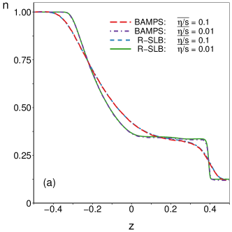
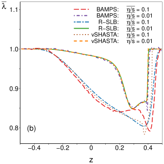
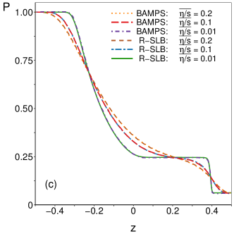
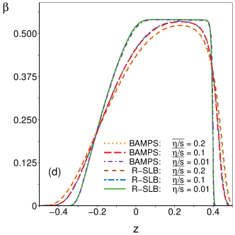
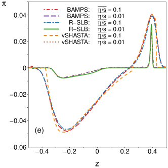
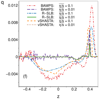
Figure 6: Comparison between the profiles obtained with the LB model with $Q_{\xi}=500$ and $N_{\Omega}=5$ and the results obtained using the BAMPS and vSHASTA methods, which were reported in Refs. Bouras et al. (2010, 2009b), for various values of $(\overline{\eta/s})$. (a) Density $n$; (b) relative fugacity $\overline{\lambda}$; (c) Pressure $P$; (d) velocity $\beta=u^{z}/u^{0}$; (e) pressure deviator $\Pi$; (f) heat flux $q$. In (b), (e) and (f), the vSHASTA results are also included.

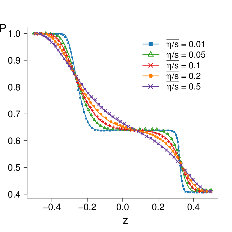
Figure 7: Comparison between the profiles of the pressure $P$, obtained with the LB model with $Q_{\xi}=500$ and $N_{\Omega}=5$ (lines), and the results obtained using the BAMPS method reported in Ref. Bouras et al. (2009a) (points), for various values of $(\overline{\eta/s})$.

In this section, we discuss the validation of our models in the regime where dissipation becomes important. We compare our simulation results with those obtained in Refs. Bouras et al. (2010, 2009a, 2009b) using two methods: the Boltzmann approach of multiparton scattering (BAMPS) model and the viscous sharp and smooth transport algorithm (vSHASTA). For the simulations presented in this section, we used the “reference model” having quadrature orders $Q_{\text{\tiny L}}=2$, $Q_{\varphi}=1$, and $Q_{\xi}=500$. The expansion of $f^{\text{\tiny(eq)}}$ was truncated at $N_{\text{\tiny L}}=1$ and $N_{\Omega}=5$.

In Fig. 6, the profiles of $n$, $\overline{\lambda}$, $P$, $\beta$, $\Pi$ and $q$ are represented for the initial conditions $(n_{\text{\tiny L}},T_{\text{\tiny L}},P_{\text{\tiny L}})=(1,1,1)$ and $(n_{\text{\tiny R}},T_{\text{\tiny R}},P_{\text{\tiny R}})=(0.125,0.5,0.0625)$, corresponding to the values used in Refs. Bouras et al. (2010); Hupp et al. (2011); Mohseni et al. (2013); Bouras et al. (2009b). Very good agreement between the results of our simulations and BAMPS is observed for the profiles of $n$, $P$ and $\beta$ when $(\overline{\eta/s})\in\{0.01,0.1,0.2\}$, where the connection between $(\overline{\eta/s})$, and the relaxation time $\tau_{\text{\tiny A-W}}$ is given in Eq. (164).

Furthermore, since the relaxation time of the Anderson-Witting model is chosen such that $(\overline{\eta/s})$ matches the BAMPS value, we note that the shear stress $\Pi$ is also in good agreement with both the vSHASTA Bouras et al. (2010, 2009b) and BAMPS data at $(\overline{\eta/s})=0.01$. At $(\overline{\eta/s})=0.1$, our simulation results for $\Pi$ are close to the BAMPS results, while the discrepancy with the vSHASTA data seems to indicate that the hydrodynamic description loses its validity. The situation is somewhat reversed for the relative fugacity $\overline{\lambda}$ (35) and the heat flux $q$. At $(\overline{\eta/s})=0.01$, the agreement between our results and the vSHASTA data is very good, while the BAMPS data exhibits a spike in $\overline{\lambda}$ near the shock front. Since in the hydrodynamic limit, the heat flux is proportional to the derivatives of $\overline{\lambda}$ [see Eq. (34b)], the spike in the profile of $\overline{\lambda}$ induces a larger peak value of $q$ near the shock front. Even though the vSHASTA method seems to be inaccurate at $(\overline{\eta/s})=0.1$, our results are still closer to the vSHASTA data as compared to the BAMPS data.

The agreement between our simulation and the vSHASTA results is not surprising. According to Eq. (53) in Ref. Bouras et al. (2010), the vSHASTA algorithm implements the heat conductivity $\lambda_{\text{\tiny heat}}$ (denoted $\kappa_{q}$ in Ref. Bouras et al. (2010)) such that $\eta/\lambda_{\text{\tiny heat}}=3T/5$, which is the same as that corresponding to the Chapman-Enskog expansion (36b). Since the value of $(\overline{\eta/s})$ is fixed in both our own and in the vSHASTA simulations to match the value of $(\overline{\eta/s})$ employed in the BAMPS simulations, it follows that the value of $\lambda_{\text{\tiny heat}}$ arising in our simulations corresponds to that employed by vSHASTA.

We attribute the strong fluctuations observed in the BAMPS result to the sensitivity of $\overline{\lambda}=n^{4}/P^{3}$ to errors in $n$ or $P$, which are prone to be present in any stochastic numerical method. Indeed, allowing $n$ and $P$ to fluctuate by some small quantities $\delta n$ and $\delta P$, it can be seen that the fluctuation in $\overline{\lambda}$ is

$$\frac{\delta\overline{\lambda}}{\overline{\lambda}}=\frac{4\delta n}{n}-\frac{3\delta P}{P}.$$ (189)

In the inviscid regime $P_{\text{\tiny C}}\simeq 0.247$ around the contact discontinuity and $P_{\text{\tiny R}}=0.0625$. This indicates that the fluctuation $\delta P$ in $P$ can be amplified by a factor between $12$ and $48$.

In Fig. 7, the pressure profile is compared with the BAMPS results reported in Ref. Bouras et al. (2009a) for higher values of $(\overline{\eta/s})$, for the following reference values Bouras et al. (2009a); Mendoza et al. (2010):

$$\widetilde{k}_{B}\widetilde{T}_{\text{\tiny ref}}=0.35\ {\rm GeV},\qquad\widetilde{P}_{\text{\tiny ref}}=5.43\ {\rm GeV}/{\rm fm}^{3},{}$$

$$\widetilde{n}_{\text{\tiny ref}}=15.514\ {\rm fm}^{-3},$$ (190)

while the reference length is $\widetilde{L}_{\text{\tiny ref}}=6.4\ {\rm fm}$. With the above quantities, $\lambda_{\text{\tiny ref}}\simeq 1.715$ and

$$\tau_{\text{\tiny A-W}}\simeq \frac{\tau_{\text{\tiny A-W};0}}{T}\left(0.865-\frac{\ln\overline{\lambda}}{4}\right),$$

$$\tau_{\text{\tiny A-W};0}\simeq 0.4405(\overline{\eta/s}).$$ (191)

In the right half of the domain, the system is initialized according to:

$$\widetilde{k}_{B}\widetilde{T}_{\text{\tiny R}}=0.35\ {\rm GeV},\qquad\widetilde{P}_{\text{\tiny R}}=2.22\ {\rm GeV}/{\rm fm}^{3},{}$$

$$\widetilde{n}_{\text{\tiny R}}=6.34\ {\rm fm}^{-3},$$ (192)

which correspond to:

$$T_{\text{\tiny R}}=1,\qquad P_{\text{\tiny R}}=0.409,\qquad n_{\text{\tiny R}}=0.409.$$ (193)

With the above values, the relative fugacity (35) takes the following values:

$$\overline{\lambda}_{\text{\tiny L}}=1,\qquad\overline{\lambda}_{\text{\tiny R}}=0.409.$$ (194)

The relaxation times in the two halves of the channel are:

$$\tau_{\text{\tiny A-W};\text{\tiny L}}\simeq 0.3811(\overline{\eta/s}),\qquad\tau_{\text{\tiny A-W};\text{\tiny R}}\simeq 0.4795(\overline{\eta/s}).$$ (195)

The simulation conditions in this case are less challenging, but this choice of parameters allows us to validate our results for the pressure profile up to $(\overline{\eta/s})=0.5$.

IV.5 Convergence test

To determine the adequate order for the quadratures at a given relaxation time, we follow Refs. Ambrus and Sofonea (2016a, b) and employ a convergence test, which is described below. In the inviscid and ballistic regimes, the profiles recovered with our LB models show a satisfactory convergence trend towards the analytic solutions. At a finite relaxation time however, as there is no analytic profile to which to compare, we can only check whether the procedure converges as we increase the order of the quadrature $Q_{\xi}$, as well as the truncation order $N_{\Omega}$ of $f^{\text{\tiny(eq)}}$. To this end, we chose the model with $Q_{\xi}=500$ and $N_{\Omega}=6$ to be the reference model with which the reference profiles are obtained. In order to test if a given model has achieved convergence, the following error measure is introduced:

$$\epsilon=\max_{j}(\epsilon_{j}),\qquad\epsilon_{j}=\left|\frac{\max_{z}\left[d_{j}(z)-d_{j,\text{\tiny\,ref}}(z)\right]}{\max_{z}[d_{j}(z)]-\min_{z}[d_{j}(z)]}\right|,$$ (196)

where the error is computed only for the macroscopic profiles $d_{j}\in\left\{n,T,\gamma\right\}$ at time $t=0.5$. The procedure selects, for a given quantity, the largest error in a single point on the whole spatial domain, for all tested profiles. We say that a model with a given $Q_{\xi}$ and $N_{\Omega}$ has achieved convergence when

$$\epsilon<\epsilon_{\text{\tiny th}}$$ (197)

for a given threshold, which we set unless otherwise stated to $\epsilon_{\text{\tiny th}}=1\%$. In Sec. IV.5.1, we employ the above test to determine the dependence of $N_{\Omega}^{\text{\tiny conv}}$ required to achieve convergence for a wide range of $(\overline{\eta/s})$, while in Sec. IV.5.2, we determine the quadrature order $Q_{\xi}^{\text{\tiny conv}}$ required to achieve convergence at various values of $\epsilon_{\text{\tiny th}}$ from the inviscid regime to the ballistic regime. These convergence tests are performed using the two initial states (166) and (193). All simulations are performed using $Z=1000$ points and $\delta t=5\times 10^{-4}$.

IV.5.1 Convergence with respect to the expansion order of $f^{\text{\tiny(eq)}}$

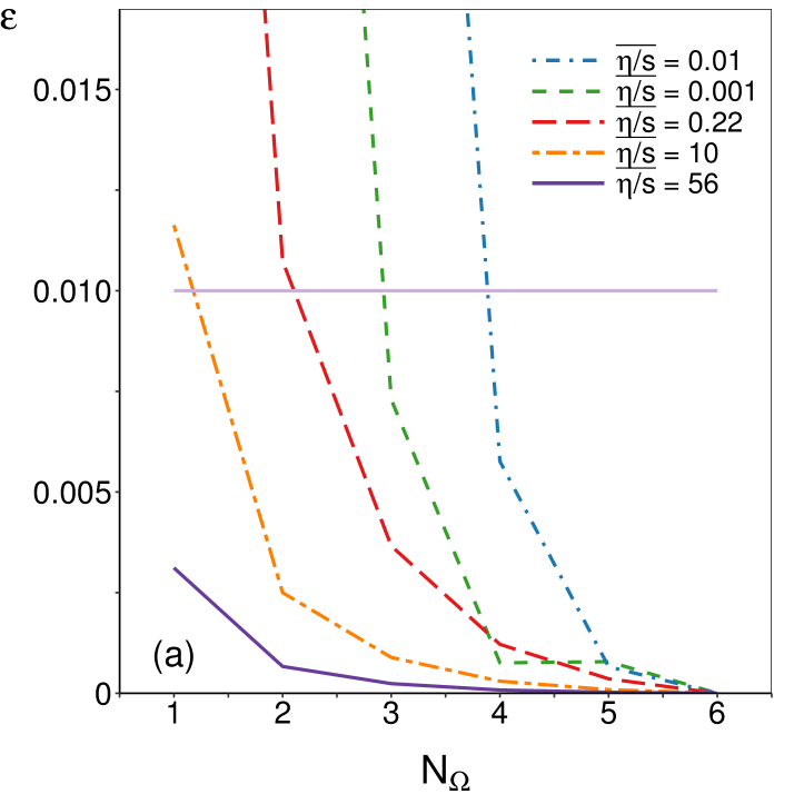
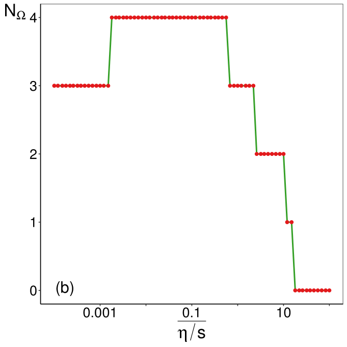
Figure 8: (a) The error $\epsilon$ (196) as a function of $N_{\Omega}$ for various values of $(\overline{\eta/s})$ ($Q_{\xi}=500$ is kept constant). The reference profiles considered here were obtained using $Q_{\xi}=500$ and $N_{\Omega}=6$. (b) The minimum expansion order $N_{\Omega}^{\text{\tiny conv}}$ required to reduce the error (196) of a model with $Q_{\xi}=500$ below the threshold $\epsilon_{\text{\tiny th}}=1\%$.

As mentioned in Sec. III.4, the order $N_{\Omega}$ at which $f^{\text{\tiny(eq)}}$ should be expanded with respect to the angular coordinates (in the case of the shock tube problem considered here, the expansion involves only $\xi=\cos\theta$) cannot be determined a priori. The expansion coefficients required to construct $f^{\text{\tiny(eq)}}$ up to $N_{\Omega}=6$ are given in Appendix A. All simulations presented in this subsection were performed using the initial state considered in Fig. 6.

Taking as a reference model the model with $Q_{\xi}=500$ and $N_{\Omega}=6$, Fig. 8(a) shows the dependence of $\epsilon$ (196) on $N_{\Omega}$ at $Q_{\xi}=500$ for various values of $(\overline{\eta/s})$. It can be seen that, for a fixed value of $(\overline{\eta/s})$, $\epsilon$ decreases as $N_{\Omega}$ is increased. Since the reference profiles correspond to $N_{\Omega}=6$, the value of $\epsilon$ at $N_{\Omega}=6$ is always $0$.

In Fig. 8(b), the dependence with respect to $(\overline{\eta/s})$ of the order $N_{\Omega}^{\text{\tiny conv}}$ required to bring $\epsilon$ below the threshold $\epsilon_{\text{\tiny th}}=1\%$ is shown. It can be seen that, for $(\overline{\eta/s})\lesssim 10^{-3}$, $N_{\Omega}^{\text{\tiny conv}}=3$. For $10^{-3}\lesssim(\overline{\eta/s})\lesssim 1$, $N_{\Omega}^{\text{\tiny conv}}$ increases to $4$. At larger values of $(\overline{\eta/s})$, the flow enters the transition regime, where the effect of collisions becomes progressively small. The value of $N_{\Omega}^{\text{\tiny conv}}$ decreases with $(\overline{\eta/s})$ down to $N_{\Omega}^{\text{\tiny conv}}=0$ as the free-streaming regime settles in at $(\overline{\eta/s})\gtrsim 18$.

According to the analysis presented in this subsection, setting $N_{\Omega}=4$ is sufficient to obtain results which are within $1\%$ error with respect to the reference profiles. Before ending this section, it is important to note that the conclusions presented in this subsection hold for the flow parameters in Eq. (166). If the initial conditions are changed such that the flow develops a larger maximum velocity, the value of $N_{\Omega}^{\text{\tiny conv}}$ may have larger values. A similar analysis should be performed whenever the flow parameters are changed, in order to accurately determine the value of $N_{\Omega}$ necessary to satisfy the convergence test (197).

IV.5.2 Convergence with respect to the quadrature order $Q_{\xi}$

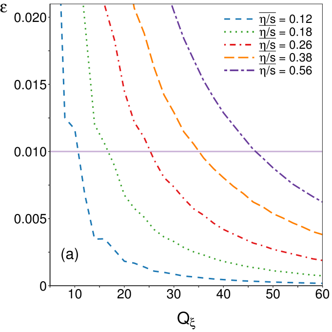
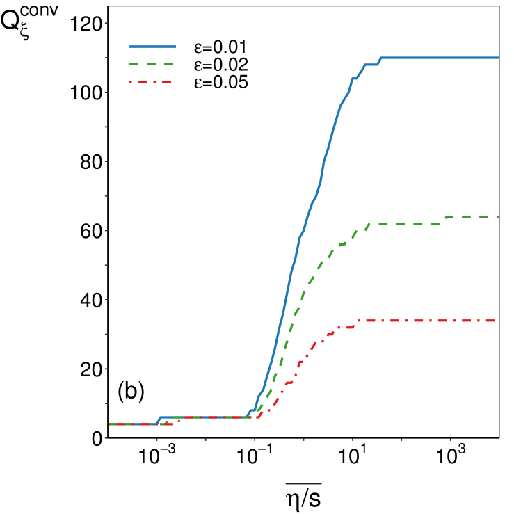
Figure 9: (a) The error $\epsilon$ (196) as a function of $Q_{\xi}$ for various values of $(\overline{\eta/s})$. The reference profiles considered here were obtained using $Q_{\xi}=500$ and $N_{\Omega}=5$. (b) The minimum quadrature order $Q_{\xi}^{\text{\tiny conv}}$ required to reduce the error (196) of a model with $N_{\Omega}={\rm min}(Q_{\xi}-1,5)$ below various values of the threshold $\epsilon_{\text{\tiny th}}$. The initial state for this analysis is given in Eq. (166).

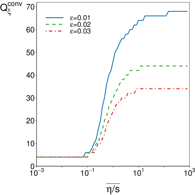
Figure 10: The minimum quadrature order $Q_{\xi}^{\text{\tiny conv}}$ required to reduce the error (196) of a model with $N_{\Omega}={\rm min}(Q_{\xi}-1,5)$ below various values of the threshold $\epsilon_{\text{\tiny th}}$ for the initial state given in Eq. (193).

Regime	Range of $(\overline{\eta/s})$	$N_{\text{\tiny vel}}$	$N_{\Omega}$
Inviscid	$(\overline{\eta/s})\lesssim 10^{-3}$	$8$	$3$
Hydrodynamic	$10^{-3}\lesssim(\overline{\eta/s})\lesssim 0.083$	$10-12$	$4$
Transition	$0.083\lesssim(\overline{\eta/s})\lesssim 18$	$12-200$	$0-4$
Ballistic	$(\overline{\eta/s})\gtrsim 18$	$220$	$0$

Table 3: Number of velocities $N_{\text{\tiny vel}}$ and expansion order $N_{\Omega}$ required in the simulation of the Sod shock tube problem with initial conditions (166) to reduce the error $\epsilon$ (196) below $\epsilon_{\text{\tiny th}}=1\%$. The error is computed for the profiles of $n$, $T$, and $\gamma$ at $t=0.5$ with respect to those obtained with $\text{R-SLB}(6;500)$ for various flow regimes.

In this section, the effects of varying the quadrature order $Q_{\xi}$ on the profiles of $n$, $T$, and $\gamma$ are investigated. The convergence test (197) is performed with respect to the reference profiles obtained using the model with $Q_{\xi}=500$ and $N_{\Omega}=5$. The initial states given by Eqs. (166) and (193) are discussed in Figs. 9 and 10, respectively.

Figure 9(a) shows the dependence of the error $\epsilon$ (196) on the quadrature order $Q_{\xi}$ for various values of $(\overline{\eta/s})$. It can be seen that $\epsilon$ decreases smoothly as $Q_{\xi}$ is increased, demonstrating the stability of our quadrature procedure.

In Fig. 9(b), the dependence on $(\overline{\eta/s})$ can be seen for the quadrature order $Q_{\xi}^{\text{\tiny conv}}$ required to reduce $\epsilon$ below the threshold error $\epsilon_{\text{\tiny th}}\in\{1\%,2\%,5\%\}$. For a fixed value of $(\overline{\eta/s})$, it can be seen that $Q_{\xi}^{\text{\tiny conv}}$ increases as $\epsilon_{\text{\tiny th}}$ is decreased. Similar features are observed in Fig. 10 for the initial state given in Eq. (193). In both cases, for a fixed value of $\epsilon_{\text{\tiny th}}$, three plateau regions and one transition region can be distinguished, which are described below for the most stringent case, namely the initial conditions in Eq. (166) and for the threshold $\epsilon_{\text{\tiny th}}=1\%$.

The inviscid limit, for which $Q_{\xi}^{\text{\tiny conv}}=4$ and $N_{\Omega}^{\text{\tiny conv}}=3$, occurs when $(\overline{\eta/s})\lesssim 10^{-3}$. In the hydrodynamic regime, [$10^{-3}\lesssim(\overline{\eta/s})\lesssim 0.083$], the non-equilibrium terms in $T^{\mu\nu}$ become important and the features of the shock become smooth, while $Q_{\xi}^{\text{\tiny conv}}$ increases to $6$ and $N_{\Omega}^{\text{\tiny conv}}$ increases to $4$. During the transition regime [$0.083\lesssim(\overline{\eta/s})\lesssim 18$], $Q_{\xi}$ increases sharply from $6$ to $\sim$100, while $N_{\Omega}^{\text{\tiny conv}}$ decreases from $4$ to $0$. Finally, in the free-streaming regime [$(\overline{\eta/s})\gtrsim 18$], $Q_{\xi}^{\text{\tiny conv}}$ reaches $110$, while $N_{\Omega}^{\text{\tiny conv}}=0$, confirming that in this regime, the particle collisions become insignificant. These results are summarized in Table 3.

We conclude that, for the initial conditions (166) and (193) and for $Z=1000$ points, a number of $Q_{\xi}\simeq 100$ quadrature points are sufficient to reduce the errors in the profiles of $n$, $T$, and $\gamma$ below the threshold of $1\%$. At high values of $(\overline{\eta/s})$, $Q_{\xi}^{\text{\tiny conv}}$ shows a strong dependence on the number $Z$ of points used to discretize the flow domain. As discussed in Sec. IV.3.2, in the free-streaming limit, the flow develops a staircaselike pattern, with the number of steps equal to $Q_{\xi}$. For a given number of fluid nodes, $Q_{\xi}$ must be increased such that the transition between these steps is smooth. If, for a fixed value of $Q_{\xi}$, the number of nodes (and hence the resolution) is increased, the staircase redevelops. A similar argument holds for the case when $Z$ is decreased.

IV.6 Summary

This section was devoted to validating the lattice Boltzmann (LB) model introduced in Sec. III in the context of the Sod shock tube problem. In order to compare our simulation results with the results obtained using the BAMPS stochastic approach and the vSHASTA hydrodynamic solver, we employed a constant shear viscosity to entropy ratio $\eta/s$.

In the inviscid regime, our models were able to recover the analytic solution of the relativistic Euler equations to very good accuracy at $(\overline{\eta/s})=10^{-4}$ [$(\overline{\eta/s})$ is the value of $\eta/s$ expressed in Planck units, as discussed in Sec. IV.1], where only $2Q_{\xi}=2\times 4=8$ velocities were required.

In order to recover the analytic solution of the free-streaming (ballistic) limit of the relativistic Boltzmann equation, the quadrature order $Q_{\xi}$ had to be increased to $110$ when $1000$ nodes were used. At smaller values of $Q_{\xi}$, the flow progresses in a staircaselike fashion, the populations corresponding to each discrete velocity propagating independently. Our simulations show that increasing the number of grid points also requires the increase of $Q_{\xi}$ in order to maintain smooth macroscopic profiles.

Our study of the dissipative regime starts while investigating the flow close to the inviscid regime. Due to the kinetic nature of our numerical approach, the systems in our simulations always exhibit some dissipation, since the transport coefficients are proportional to the relaxation time $\tau_{\text{\tiny A-W}}$, which has to remain finite in order for the simulations to be stable. In the vicinity of the shock front and contact discontinuity, the flow profiles can develop discontinuities and the non-equilibrium quantities (heat flux $q$ and shear stress $\Pi$) become non-negligible, since they are proportional to the gradients of the macroscopic fields. The magnitudes of $q$ and $\Pi$ can be estimated analytically by considering their integrated value over the range where they are non-negligible. A comparison between our numerical results and the analytic prediction indicates that our numerical scheme is consistent with the Chapman-Enskog prediction for the transport coefficients (heat conductivity and shear viscosity), while the analytic results corresponding to the Grad prediction for the transport coefficients are in visible disagreement with our numerical results.

The final validation test that we considered was a comparison with the data obtained using the BAMPS stochastic method and the vSHASTA hydrodynamics solver Bouras et al. (2010, 2009a, 2009b). In order to correlate our simulations with the simulations performed in these references, the relaxation time was implemented such that the viscosity to entropy ratio $(\overline{\eta/s})$, expressed in Planck units, matched the one employed therein. This required as an input the analytic expression for the shear viscosity. Based on our previous investigation of the dissipative effects in the nearlyinviscid regime, our model was implemented starting from the Chapman-Enskog values for the shear viscosity. Good agreement was in general observed for $(\overline{\eta/s})$ up to $0.5$. There is some discrepancy between our simulation results and the BAMPS data for the heat flux, our results being closer to the vSHASTA prediction. This can be explained since in the vSHASTA implementation, the heat conductivity is fixed at the value predicted through the Chapman-Enskog procedure for the Anderson-Witting model for ultrarelativistic particles, which coincides with the model employed in our implementation. The number of velocities required to obtain good agreement with the BAMPS data is less than $20$ at $(\overline{\eta/s})\lesssim 0.1$. At $(\overline{\eta/s})\simeq 0.5$, the flow enters the rarefied regime and a significantly larger number of quadrature points is required, as indicated by Figs. 9 and 10.

V One-dimensional boost-invariant expansion

We now consider the evolution with respect to the proper time $\tau$ of the distribution function corresponding to a fluid which is homogeneous with respect to the spatial coordinates of the Milne coordinate system introduced in Sec. II.6 from an initial equilibrium state, described by the Maxwell-Jüttner distribution. This assumption represents the implementation of the one-dimensional boost-invariant expansion model (Bjorken flow). This setup is used to test the LB models introduced in Sec. III throughout the whole rarefaction spectrum. Our models are validated against analytic solutions in the inviscid and ballistic regimes, as well as against numerical solutions of the second-order hydrodynamics equations in the viscous regime. In the transition regime, our numerical results are validated by comparison with the semianalytic results reported in Ref. Florkowski et al. (2013).

The nondimensionalization convention and initial state are discussed in Sec. V.1. The macroscopic equations are discussed in Sec. V.2. The subsequent analysis is performed separately for the parton gas (flow at vanishing chemical potential) and ideal gas ($P=nT$) assumptions, which are discussed in Secs. V.3 and V.4, respectively. A test of the convergence of our numerical results with respect to the quadrature order is performed in Sec. V.5. Section V.6 summarizes our results and concludes this section.

V.1 Nondimensionalization convention and initial setup

The nondimensionalization procedure employed in this section uses as reference quantities the initial proper time $\widetilde{\tau}_{\rm ref}=\widetilde{\tau}_{0}=(0.25/\widetilde{c})\ {\rm fm}$ and the initial system temperature $\widetilde{T}_{\rm ref}=\widetilde{T}_{0}$. Two particular values for $\widetilde{T}_{0}$ are considered, namely $\widetilde{k}_{B}\widetilde{T}_{0}=0.3\ {\rm GeV}$ and $\widetilde{k}_{B}\widetilde{T}_{0}=0.6\ {\rm GeV}$. The relaxation time $\tau_{\text{\tiny A-W}}$ is fixed by imposing a constant shear viscosity to entropy ratio $(\overline{\eta/s})$, expressed in Planck units, such that:

$$\tau_{\text{\tiny A-W}}=\frac{\tau_{\text{\tiny A-W};0}}{T}\left[1-\frac{\ln(\overline{\lambda}\lambda_{\text{\tiny ref}})}{4}\right],\quad\tau_{\text{\tiny A-W};0}=\frac{5\widetilde{\hbar}(\overline{\eta/s})}{\widetilde{\tau}_{0}\widetilde{k}_{B}\widetilde{T}_{0}},$$ (198)

where the relative fugacity $\overline{\lambda}$ and reference fugacity $\lambda_{\text{\tiny ref}}$ are defined in Eq. (138). More details on how to arrive at Eq. (198) can be found in Sec. IV.1. The reference particle number density $\widetilde{n}_{\text{\tiny ref}}=\widetilde{n}_{0}$ is taken to be the particle number density at initial time, such that $n_{0}=1$ and $\overline{\lambda}(\tau=1)=1$. Throughout this section, only the case when the chemical potential vanishes at initial time is considered, i.e., $\lambda_{\text{\tiny ref}}=1$, such that the initial (reference) particle number density is determined by the initial temperature through:

$$\widetilde{n}_{\text{\tiny ref}}=\frac{g_{s}}{\pi^{2}}\left(\frac{\widetilde{k}_{B}\widetilde{T}_{\text{\tiny ref}}}{\widetilde{\hbar}\widetilde{c}}\right)^{3},$$ (199)

where $g_{s}=16$ is the gluon number of degrees of freedom.

Taking into account the above non-dimensionalization conventions, the distribution function at initial time takes the following form:

$$f(\tau=1)=\frac{1}{8\pi}e^{-p}.$$ (200)

A generalization of the above initial condition is to account for possible anisotropies in the initial particle distribution function, e.g., by employing the Romatschke-Strickland anisotropic distribution Romatschke and Strickland (2003); Florkowski et al. (2013). For simplicity, we only consider the isotropic initial state given by Eq. (200) and defer the study of the anisotropic case for future work.

V.2 Macroscopic equations

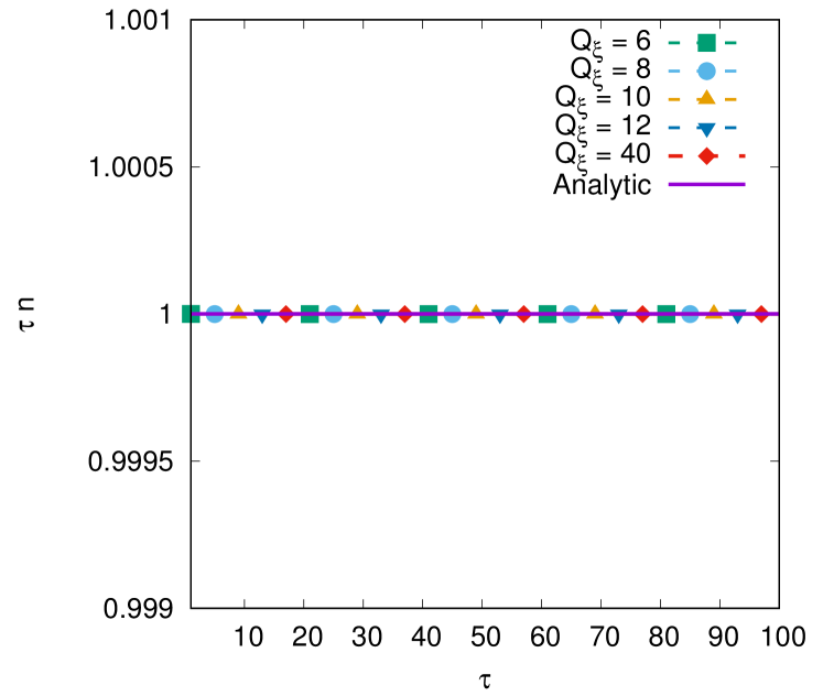
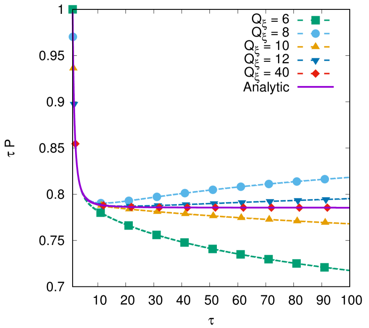
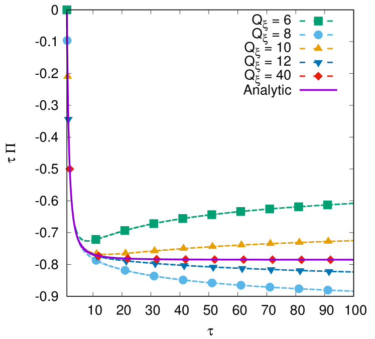
Figure 11: Evolution of $\tau n$ (a), $\tau P$ (b), and $\tau\Pi$ (c) with respect to $\tau$. The $\tau$ factor is included in order to highlight the asymptotic limits (207). The numerical results corresponding to various $Q_{\xi}$ (dashed lines and points) are compared to the analytic solutions (solid lines) given in Eqs. (202) and (206), which are overlapped with the $Q_{\xi}=40$ curves.

Using the connection coefficients given in Eq. (52), the conservation equations $\nabla_{{\hat{\alpha}}}N^{\hat{\alpha}}=0$ and $\nabla_{{\hat{\sigma}}}T^{{\hat{\alpha}}{\hat{\sigma}}}=0$ reduce to:

$$\partial_{\tau}(N^{\hat{\tau}}\tau)= \ 0,$$

$$\partial_{\tau}(T^{{\hat{\tau}}{\hat{\tau}}}\tau)+T^{{\hat{\eta}}_{M}{\hat{\eta}}_{M}}= \ 0,{}$$

$$\partial_{\tau}(T^{{\hat{\tau}}{\hat{x}}}\tau)=\partial_{\tau}(T^{{\hat{\tau}}{\hat{y}}}\tau)= \ 0,{}$$

$$\partial_{\tau}(T^{{\hat{\tau}}{\hat{\eta}}_{M}}\tau^{2})= \ 0.$$ (201)

The equations on the last two lines above are automatically satisfied by setting $T^{{\hat{\tau}}{\hat{x}}}=T^{{\hat{\tau}}{\hat{y}}}=T^{{\hat{\tau}}{\hat{\eta}}_{M}}=0$, such that the stress-energy tensor takes the form in Eq. (57) and the Landau velocity is $u^{\hat{\alpha}}=(1,0,0,0)^{T}$ (54) at all times $\tau>\tau_{0}$. In this case, the Landau and Eckart frames coincide, such that $N^{\hat{\tau}}=n$ is just the particle number density. Furthermore, the first relation in Eq. (201) yields

$$n=\frac{1}{\tau},$$ (202)

while the second line in (201) reduces to:

$$4P^{1/4}\partial_{\tau}(\tau P^{3/4})+\Pi=0.$$ (203)

In the inviscid regime, Eq. (203) can be solved by setting $\Pi=0$, giving the Bjorken ideal flow solution Bjorken (1983):

$$P=\frac{1}{\tau^{4/3}},\qquad T=\frac{1}{\tau^{1/3}},$$ (204)

where the expression for $T=P/n$ was obtained by noting that $n$ is given by Eq. (202). It can be seen that $\lambda=1$ for all values of $\tau$, such that in the inviscid regime, the chemical potential vanishes at all times.

In the free-streaming regime, the Boltzmann equation (53) subject to the initial condition (200) imposed at $\tau=1$ has the following exact solution:

$$f(\tau;p,\xi)=\frac{1}{8\pi}\exp\left(-p\sqrt{1+(\tau^{2}-1)\xi^{2}}\right).$$ (205)

The macroscopic quantities $P=\frac{1}{3}T^{{\hat{\tau}}{\hat{\tau}}}$ and $\mathcal{P}_{L}=T^{{\hat{\eta}}_{M}{\hat{\eta}}_{M}}=P-\Pi$ can be computed by direct integration of Eq. (205):

$$P= \frac{1}{2}\left[\frac{\arctan\left(\sqrt{\tau^{2}-1}\right)}{\sqrt{\tau^{2}-1}}+\frac{1}{\tau^{2}}\right],$$

$$\mathcal{P}_{L}= \frac{3}{2}\frac{1}{\tau^{2}-1}\left[\frac{\arctan\left(\sqrt{\tau^{2}-1}\right)}{\sqrt{\tau^{2}-1}}-\frac{1}{\tau^{2}}\right],$$ (206)

As $\tau\rightarrow\infty$, the following asymptotic behavior is achieved:

$$\lim_{\tau\rightarrow\infty}(\tau P)=-\lim_{\tau\rightarrow\infty}(\tau\Pi)=\frac{\pi}{4}.$$ (207)

The solution (206) is compared with our numerical results in Fig. 11, highlighting the asymptotic behavior (206) by representing the quantities $\tau n$, $\tau P$, and $\tau\Pi$. It can be seen that the numerical results improve as the quadrature $Q_{\xi}$ is increased, with clear deviations from the analytic solutions of $P$ and $\Pi$ at $Q_{\xi}\lesssim 12$, while at $Q_{\xi}=40$, the agreement with the analytic solution is excellent. It is noteworthy that the evolution of $\tau n$ is exactly recovered even when $Q_{\xi}=6$. The expansion order of $f^{\text{\tiny(eq)}}$ is $N_{\Omega}=5$ and the time step was set to $\delta\tau=10^{-3}$.

In the viscous regime, the Chapman-Enskog procedure shows that the shear stress $\Pi$ is given up to first order by:

$$\Pi=4\eta\nabla^{\langle{\hat{x}}}u^{{\hat{x}}\rangle}=-\frac{4\eta}{3}\Gamma^{\hat{\alpha}}{}_{{\hat{\tau}}{\hat{\alpha}}}=-\frac{4\eta}{3\tau},$$ (208)

where $\Gamma^{\hat{\alpha}}{}_{{\hat{\tau}}{\hat{\alpha}}}=1/\tau$ according to Eq. (52). The equation for the pressure (203) becomes:

$$4P^{1/4}\partial_{\tau}(\tau P^{3/4})=\frac{16P}{15\tau}\tau_{\text{\tiny A-W}},$$ (209)

where the Chapman-Enskog expression (36b) for the shear viscosity $\eta$ was employed. It can be seen that $\Pi$ takes the value $-4\eta/3$ at initial time ($\tau=1$), which is incompatible with the initial condition (200), according to which the fluid is in thermal equilibrium when $\tau=1$. Thus, the constitutive equation for $\Pi$ must be upgraded to an evolution equation by employing a secondorder hydrodynamics formulation, giving rise to the following system of equations Jaiswal (2013a); Florkowski et al. (2013):

$$3\tau\partial_{\tau}P+4P= -\Pi,$$

$$\tau_{\Pi}\partial_{\tau}\Pi+\Pi= -\frac{4\eta}{3\tau}-\beta_{\Pi}\frac{\tau_{\Pi}}{\tau}\Pi,$$ (210)

where $\tau_{\Pi}=\tau_{\rm A-W}$ and $\beta_{\Pi}=38/21$ for the Anderson-Witting approximation of the collision term Jaiswal (2013a); Florkowski et al. (2013). For completeness, a derivation of the above relations is presented in Appendix C using a moment-based method.

V.3 Parton gas model

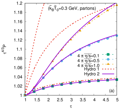
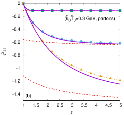
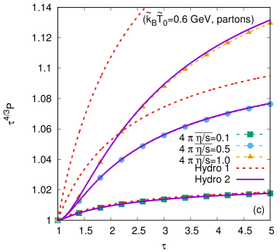
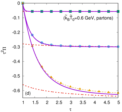
Figure 12: Time evolution of (left) $\tau^{4/3}P$ and (right) $\tau^{2}\Pi$ for $\widetilde{k}_{B}\widetilde{T}_{0}=0.3\ {\rm GeV}$ (top) and $0.6\ {\rm GeV}$ (bottom) for $4\pi(\overline{\eta/s})\in\{0.1,0.5,1.0\}$ for partons ($\mu=0$). The numerical results (dotted lines and points) are compared with the first-order (dotted lines) and second-order (solid lines) hydrodynamics results obtained from Eqs. (215) and (216), respectively. The factors $\tau^{4/3}$ and $\tau^{2}$ multiplying $P$ and $\Pi$ are inspired from the form of the first-order hydrodynamics solutions (215).

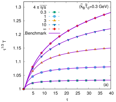
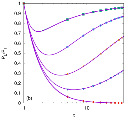
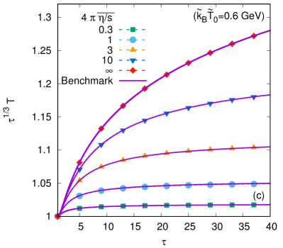
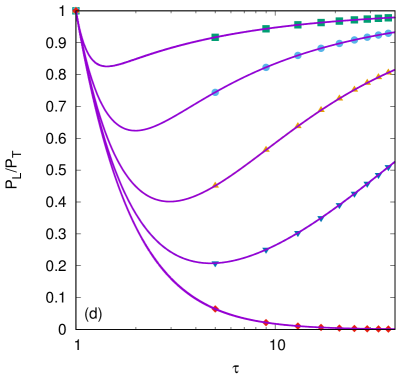
Figure 13: Evolution with respect to $\tau$ of (left) $T$ and (right) ratio $\mathcal{P}_{L}/\mathcal{P}_{T}$ of the longitudinal to the transverse pressure, for $\widetilde{k}_{B}\widetilde{T}_{0}=0.3\ {\rm GeV}$ (top) and $0.6\ {\rm GeV}$ (bottom), for various values of $(\overline{\eta/s})$, under the assumption of vanishing chemical potential discussed in Sec. V.3. The numerical results (dotted lines and points) are validated using benchmark results (solid lines) as follows: for $(\overline{\eta/s})=\infty$, the analytic formulas (206) and (211) are used; at $4\pi(\overline{\eta/s})=0.3$, the numerical solution of the second order hydrodynamics equations (216) is used; when $4\pi(\overline{\eta/s})\in\{1,3,10\}$, the semi-analytic solution reported in Ref. Florkowski et al. (2013) is represented.

In the parton gas model, the fluid undergoing boost-invariant expansion is dominated by gluons, which are considered to evolve at vanishing chemical potential Florkowski et al. (2013). In this model, $\overline{\lambda}=1$ for all $\tau\geq 1$. This can be achieved by constructing $f^{\text{\tiny(eq)}}$ and $\tau_{\text{\tiny A-W}}$ with $n^{\text{\tiny(eq)}}=T^{3}$, where the temperature is related to the isotropic pressure $P=\frac{1}{3}T^{{\hat{\tau}}{\hat{\tau}}}$ through Florkowski et al. (2013):

$$T^{\text{\tiny(eq)}}=P^{1/4}\equiv T,\qquad n^{\text{\tiny(eq)}}=P^{3/4},$$

$$f^{\text{\tiny(eq)}}=\frac{1}{8\pi}\exp\left(-\frac{p^{\hat{\tau}}}{P^{1/4}}\right),$$ (211)

where the first relation also defines the fluid temperature $T$, such that $\tau_{\text{\tiny A-W}}$ (198) becomes

$$\tau_{\text{\tiny A-W}}=\frac{\tau_{\text{\tiny A-W};0}}{P^{1/4}},\qquad\tau_{\text{\tiny A-W};0}=\frac{5\widetilde{\hbar}(\overline{\eta/s})}{\widetilde{\tau}_{0}\widetilde{k}_{B}\widetilde{T}_{0}}.$$ (212)

It is noteworthy that the parton density $n$ is not conserved. Its evolution is governed by (241):

$$\partial_{\tau}(\tau n)=-\frac{P^{1/4}}{\tau_{\text{\tiny A-W};0}}(n-P^{3/4}).$$ (213)

In the context of first-order hydrodynamics, Eq. (203) can be simplified by substituting $\Pi$ from Eq. (208):

$$\frac{\partial_{\tau}(\tau P^{3/4})}{(\tau P^{3/4})^{2/3}}=\frac{4\tau_{\text{\tiny A-W};0}}{15\tau^{5/3}}.$$ (214)

The above equation can be solved analytically, such that $P$ and $\Pi$ are given by

$$P= \frac{1}{\tau^{4/3}}\left[1+\frac{2\tau_{\text{\tiny A-W};0}}{15}\left(1-\frac{1}{\tau^{2/3}}\right)\right]^{4},$$

$$\Pi= -\frac{16\tau_{\text{\tiny A-W};0}}{15\tau^{2}}\left[1+\frac{2\tau_{\text{\tiny A-W};0}}{15}\left(1-\frac{1}{\tau^{2/3}}\right)\right]^{3}.$$ (215)

In the case of the second-order hydrodynamics equations, the following system must be solved:

$$\partial_{\tau}P= -\frac{4}{3\tau}P-\frac{1}{3\tau}\Pi,$$

$$\partial_{\tau}\Pi= -\frac{P^{1/4}}{\tau_{\text{\tiny A-W};0}}\Pi-\frac{38}{21\tau}\Pi-\frac{16}{15\tau}P.$$ (216)

Further analytic development seems difficult to achieve, however the above system can be easily integrated numerically.

Finally, outside the hydrodynamic regime, a semianalytic formula was derived in Ref. Florkowski et al. (2013), which allows the temperature $T$, parton number density $n$, and longitudinal pressure $\mathcal{P}_{L}$ to be computed iteratively via the following equations:

$$T^{4}(\tau)= D(\tau,1)\frac{\mathcal{H}(\tau^{-1})}{\mathcal{H}(1)}$$

$$+\int_{1}^{\tau}\frac{T^{4}(\tau^{\prime})d\tau^{\prime}}{2\tau_{\text{\tiny A-W}}(\tau^{\prime})}\,D(\tau,\tau^{\prime})\mathcal{H}\left(\frac{\tau^{\prime}}{\tau}\right),$$

$$n(\tau)= \frac{1}{\tau}\left[D(\tau,1)+\int_{1}^{\tau}\frac{T^{3}(\tau^{\prime})\tau^{\prime}d\tau^{\prime}}{\tau_{\text{\tiny A-W}}(\tau^{\prime})}D(\tau,\tau^{\prime})\right],$$

$$\mathcal{P}_{L}(\tau)= 3\left[D(\tau,1)\frac{\mathcal{H}_{L}(\tau^{-1})}{\mathcal{H}(1)}.\right.$$

$$\left.+\int_{1}^{\tau}\frac{T^{4}(\tau^{\prime})d\tau^{\prime}}{2\tau_{\text{\tiny A-W}}(\tau^{\prime})}\,D(\tau,\tau^{\prime})\mathcal{H}_{L}\left(\frac{\tau^{\prime}}{\tau}\right)\right],$$ (217)

where the damping function $D(\tau_{2},\tau_{1})$ and the $\mathcal{H}$ and $\mathcal{H}_{L}$ functions are given by:

$$D(\tau_{2},\tau_{1})= \exp\left[-\frac{1}{\tau_{\text{\tiny A-W;0}}}\int_{\tau_{1}}^{\tau_{2}}d\tau^{\prime\prime}\,T(\tau^{\prime\prime})\right],$$

$$\mathcal{H}(y)= y^{2}+\frac{\arctan\sqrt{y^{-2}-1}}{\sqrt{y^{-2}-1}},$$

$$\mathcal{H}_{L}(y)= y^{2}\frac{d}{dy}\left[\frac{\mathcal{H}(y)}{y}\right].$$ (218)

The temperature profile $T_{(n)}$ at the $n$th iteration is found by inserting $T_{(n-1)}$ on the right-hand side of the first of Eqs. (217). This iterative method was started with the ideal flow solution $T_{(0)}=\tau^{-1/3}$. The numerical integrals were computed using the trapezoidal rule and the integration domain comprised $975$ equidistant intervals of length $\delta\tau=0.04$ distributed between $\tau=1$ and $\tau=\tau_{f}=40$. The algorithm was stopped when the $L_{2}$ norm of the difference $T_{(n)}-T_{(n-1)}$ between the temperature profiles obtained after $n$ and $n-1$ iterations decreased below the tolerance threshold $10^{-7}$:

$$L_{2}^{(n)}=\sqrt{\int_{1}^{\tau_{f}}\frac{d\tau}{\tau_{f}-1}[T_{(n)}(\tau)-T_{(n-1)}(\tau)]^{2}}\leq 10^{-7}.$$ (219)

The validity of the first- and second-order hydrodynamics theories is tested in Fig. 12. It can be seen that the second-order theory accurately captures the early time relaxation of $\Pi$ (right column) from $\Pi=0$ at $\tau=1$ to the value predicted by the first-order theory, which becomes accurate at $\tau\gtrsim\tau_{0}+5[4\pi(\overline{\eta/s})]$ for sufficiently small values of $4\pi(\overline{\eta/s})$. The limitations of the first-order hydrodynamics theory become evident when considering the evolution of the pressure (left column in Fig. 12). At $4\pi(\overline{\eta/s})\gtrsim 0.5$, the first-order theory presents significant deviations from the second-order theory and the numerical results.

While accurate at $4\pi(\overline{\eta/s})\lesssim 0.5$, the second-order hydrodynamics formulation seems to lose validity when $4\pi(\overline{\eta/s})\gtrsim 1$, as shown in Fig. 12. For $4\pi(\overline{\eta/s})\in\{1,3,10\}$, Fig. 13 shows a comparison of our results for the temperature $T$ and the ratio $\mathcal{P}_{L}/\mathcal{P}_{T}$ between the longitudinal and the numerical iterative solution of Eq. (217). Excellent agreement is found at both $\widetilde{k}_{B}\widetilde{T}_{0}=0.3\ {\rm GeV}$ and $0.6\ {\rm GeV}$. Also in Fig. 13, a comparison with the analytic solution (206) in the ballistic regime is presented, showing that our models can recover the flow features in this regime as well.

The parameters for the simulations discussed in this section were $Q_{\xi}=40$, $N_{\Omega}=5$ and $\delta\tau=10^{-3}$.

V.4 Ideal gas model

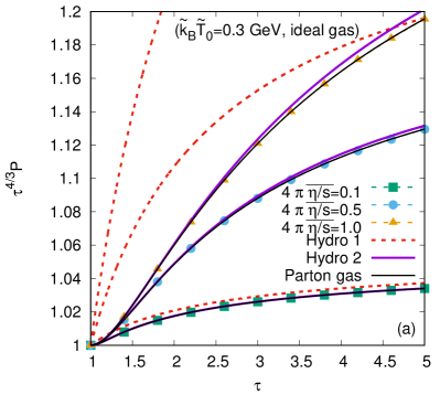
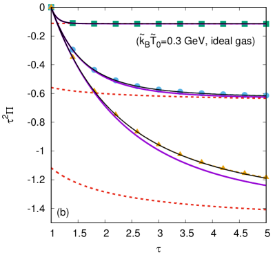
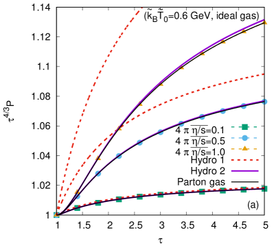
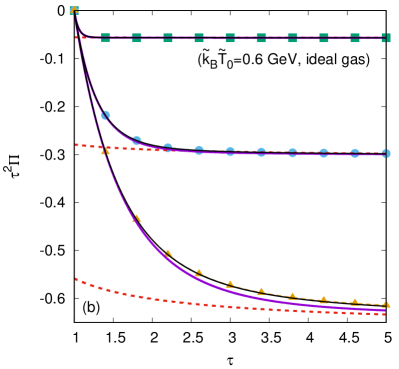
Figure 14: Time evolution of (left) $P$ and (right) $\Pi$ for $4\pi(\overline{\eta/s})\in\{0.1,0.5,1\}$ for initial temperatures $\widetilde{k}_{B}\widetilde{T}_{0}=0.3\ {\rm GeV}$ (top) and $0.6\ {\rm GeV}$ (bottom). The various curves show the numerical results obtained using LB for the cases of the ideal gas (dotted lines and points) and of the gas of partons (solid black lines), as well as the solutions of the first (dotted lines) and second (solid purple lines) hydrodynamics equations (221) and (222) for the ideal gas. The ideal and parton gas results seem to be overlapped for all tested values of $(\overline{\eta/s})$ and $\widetilde{T}_{0}$.

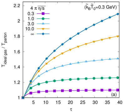
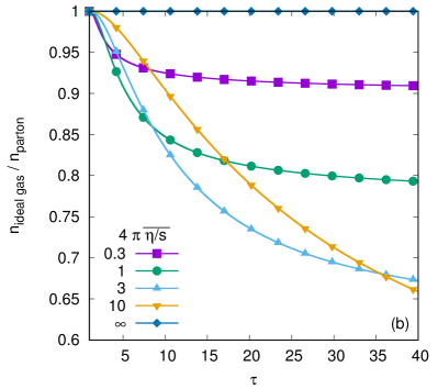
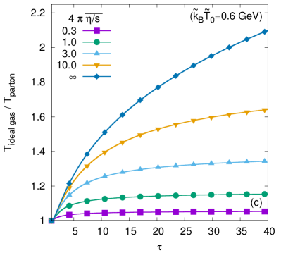
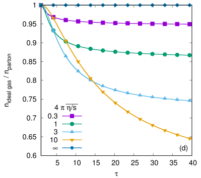
Figure 15: Evolution of the ratios (left) $T_{\text{ideal gas}}/T_{\text{partons}}$ and (right) $n_{\text{ideal gas}}/n_{\text{partons}}$ of the temperatures and densities obtained for the ideal ($P=nT$) and parton ($\mu_{\rm eq}=0$) gases, for $\widetilde{k}_{B}\widetilde{T}_{0}=0.3\ {\rm GeV}$ (top) and $0.6\ {\rm GeV}$ (bottom) for $4\pi(\overline{\eta/s})\in\{0.3,1,3,10,\infty\}$.

Let us now consider that the medium is an ideal gas, such that $P=nT$ and $n^{\text{\tiny(eq)}}=n$ in Eq. (241), where $n$ is given by Eq. (202), while $T=P/n=\tau P$. In this case, $f^{\text{\tiny(eq)}}$ is computed via Eq. (27), while $\tau_{\text{\tiny A-W}}$ (198) becomes

$$\tau_{\text{\tiny A-W}}=\frac{\tau_{\text{\tiny A-W};0}}{\tau P}\left[1+\ln(\tau P^{3/4})\right],\quad\tau_{\text{\tiny A-W};0}=\frac{5\widetilde{\hbar}(\overline{\eta/s})}{\widetilde{\tau}_{0}\widetilde{k}_{B}\widetilde{T}_{0}}.$$ (220)

In order to derive the time evolution of $P$ predicted via the first-order dissipative hydrodynamics approximation, Eq. (220) can be substituted into Eq. (209), giving the following system of equations:

$$\frac{\partial_{\tau}(P\tau^{4/3})}{\frac{4}{3}+\ln(P\tau^{4/3})}= \frac{4\tau_{\text{\tiny A-W};0}}{15\tau^{5/3}},$$

$$\Pi= -\frac{4\tau_{\text{\tiny A-W};0}}{5\tau^{2}}\left[\frac{4}{3}+\ln(P\tau^{4/3})\right].$$ (221)

In the second-order hydrodynamics approach, the following system of equations must be solved:

$$\partial_{\tau}P= -\frac{4}{3\tau}P-\frac{1}{3\tau}\Pi,$$

$$\partial_{\tau}\Pi= -\frac{\tau P}{\tau_{\text{\tiny A-W};0}[1+\ln(\tau P^{3/4})]}\Pi-\frac{38}{21\tau}\Pi-\frac{16}{15\tau}P.$$ (222)

The solution of the above system is obtained via numerical integration.

Figure 14 validates our implementation by comparing the numerical results obtained with our LB models with the predictions of the first- and second-order hydrodynamics equations (221) and (222), respectively. As in the case of the parton gas, the first-order hydrodynamics formulation cannot account for a vanishing $\Pi$ (right column) at initial time $\tau=1$ and is thus inaccurate for $\tau\lesssim 1+5[4\pi(\overline{\eta/s})]$. Furthermore, it loses applicability when $4\pi(\overline{\eta/s})\gtrsim 0.5$, especially when considering the evolution of the isotropic pressure $P$ (left column). The second-order hydrodynamics formulation provides a good match for the early time evolution of both $\Pi$ and $P$ and seems to lose validity when $4\pi(\overline{\eta/s})\gtrsim 1$. Also in Fig. 14, a comparison between the ideal gas (dotted lines and points) and the parton gas (solid black lines) shows that the evolution of $P$ and $\Pi$ is (surprisingly) extremely similar in the two models.

In Fig. 15, the time evolution predicted in the ideal gas ($P=nT$) and parton gas ($\mu=0$) models is further compared by considering the evolution of the temperature $T$ (left) and number density $n$ (right). It can be seen that the temperature of the ideal gas undergoing the longitudinal boost-invariant expansion always exceeds the temperature of the parton gas. The ratio $n_{\text{ideal gas}}/n_{\text{partons}}$ at fixed values for $\tau$ decreases when $4\pi(\overline{\eta/s})\lesssim 3$ from $1$ in the perfect fluid regime [$(\overline{\eta/s})\rightarrow 0$] towards a minimum value, after which it increases for $4\pi(\overline{\eta/s})\gtrsim 10$ towards $1$ in the ballistic regime [$(\overline{\eta/s})\rightarrow\infty$].

V.5 Convergence test

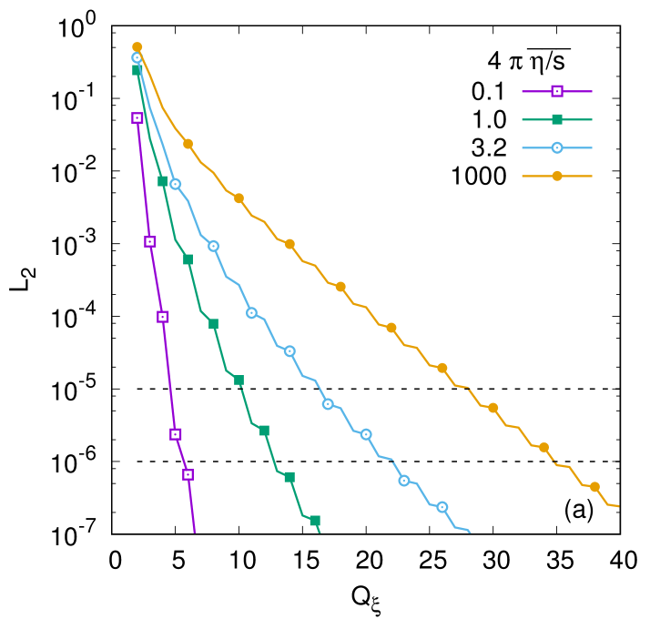
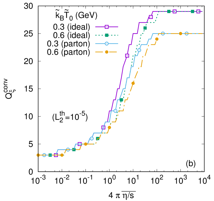
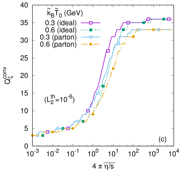
Figure 16: (a) Maximum $L_{2}$ norm (224) as a function of $Q_{\xi}$ for $\widetilde{k}_{B}\widetilde{T}_{0}=0.3\ {\rm GeV}$, under the assumption of a parton gas ($\mu=0)$. (b),(c) Dependence with respect to $4\pi(\overline{\eta/s})$ of $Q_{\xi}^{\rm conv}$ for $L_{2}^{\text{\tiny th}}=10^{-5}$ (b) and $L_{2}^{\text{\tiny th}}=10^{-6}$ (c), obtained for $\widetilde{k}_{B}\widetilde{T}_{0}\in\{0.3\ {\rm GeV},0.6\ {\rm GeV}\}$, for both the parton and ideal gases. The $L_{2}$ norm is computed with respect to the reference model $\text{R-SLB}(5;100)$.

Regime	Range of $4\pi(\overline{\eta/s})$	$N_{\text{\tiny vel}}$
Inviscid	$4\pi(\overline{\eta/s})\lesssim 10^{-3}$	$6$
Hydrodynamic	$10^{-3}\lesssim 4\pi(\overline{\eta/s})\lesssim 0.05$	$10$
Transition	$0.05\lesssim 4\pi(\overline{\eta/s})\lesssim 1000$	$10$–$66$
Ballistic	$4\pi(\overline{\eta/s})\gtrsim 1000$	$66$

Table 4: Number of velocities $N_{\text{\tiny vel}}$ required in the simulation of the Bjorken flow in order to reduce below $L_{2}^{\text{\tiny th}}=10^{-6}$ the $L_{2}$ norm for the evolution of $n$, $P$, $T$, and $\Pi$ for a parton gas ($\mu=0$) at $\widetilde{k}_{B}\widetilde{T}_{0}=0.3\ {\rm GeV}$ for various flow regimes. The reference model is $\text{R-SLB}(5;100)$.

In order to assess the efficiency of our implementation, we consider a convergence test similar to that employed in Sec. IV.5 in the context of the Sod shock tube. Since the spatial dependence of the macroscopic fields is trivial, it is convenient to consider the $L_{2}$ norm of the time evolution of the macroscopic fields $n$, $P$, $T$, and $\Pi$ with respect to the results obtained with the reference model $\text{R-SLB}(5;100)$ having $N_{\Omega}=5$ and $Q_{\xi}=100$. Denoting by $n_{\rm ref}$, etc., the profiles obtained using the reference model, the $L_{2}$ norm for the evolution of the macroscopic field $A\in\{n,T,P,\Pi\}$ is computed using

$$L_{2}(A)=\sqrt{\int_{1}^{\tau_{f}}\frac{d\tau}{\tau_{f}-1}\,[A(\tau)-A_{\rm ref}(\tau)]^{2}},$$ (223)

where $\tau_{f}=40$. We considered that convergence was achieved when

$$L_{2}\leq L_{2}^{\text{\tiny th}},\qquad L_{2}={\rm max}_{A}[L_{2}(A)],$$ (224)

where $L_{2}^{\text{\tiny th}}\in\{10^{-5},10^{-6}\}$.

Figure 16(a) shows the decrease of $L_{2}$ with $Q_{\xi}$ for various values of $(\overline{\eta/s})$. It can be seen that as $(\overline{\eta/s})$ is increased, more quadrature points are required in order to achieve the same $L_{2}$ error norm. Figures 16(b) and 16(c) show the minimum quadrature order $Q_{\xi}^{\rm conv}$ required to achieve (224) as a function of $4\pi(\overline{\eta/s})$ between the inviscid limit $10^{-3}$, where $Q_{\xi}^{\rm conv}=3$, and the ballistic limit $10^{4}$, where $Q_{\xi}^{\rm conv}=25$ for $L_{2}^{\text{\tiny th}}=10^{-5}$ (b) and $Q_{\xi}^{\rm conv}=33$ for $L_{2}^{\text{\tiny th}}=10^{-6}$ (c). The convergence orders are computed separately for $\widetilde{k}_{B}\widetilde{T}_{0}=0.3\ {\rm GeV}$ and $0.6\ {\rm Gev}$, as well as for the ideal and parton gases. The results for the convergence test with $L_{2}^{\text{\tiny th}}=10^{-6}$ corresponding to a parton gas at initial temperature $\widetilde{k}_{B}\widetilde{T}_{0}=300\ {\rm GeV}$ are summarized in Table 4.

V.6 Summary

In this section, the LB models introduced in Sec. III were employed to investigate the one-dimensional boost invariant (Bjorken) flow in the Milne coordinate system. Our models were validated by comparison with analytic solutions in the inviscid and ballistic regimes, as well as with the numerical solution of the second-order hydrodynamics at finite relaxation times. In the transition regime, our models were validated by comparison with a semi-analytic solution, constructed using an iterative process. All comparisons show that our models are capable of accurately reproducing the benchmark data. Aside from the vanishing chemical potential case considered in Ref. Florkowski et al. (2013), corresponding to a parton gas comprised of gluons, we presented for comparison an analysis of the case when the fluid obeys the ideal gas law $P=nT$, highlighting a slower temperature decrease compared to the parton gas model.

VI Summary and conclusion

In this paper, a relativistic lattice Boltzmann (LB) model was developed for the simulation of flows of ultrarelativistic particles. The momentum space is discretized by using a set of quadrature rules, giving rise to off-grid velocity sets. As the procedure for selecting the velocities is analytical, the set can be extended up to arbitrarily high orders. This in turn allows flows with any degree of rarefaction (i.e., the entire range of the relaxation time) to be described accurately. The model is validated in the contexts of the Sod shock tube problem and of the Bjorken flow.

In the inviscid limit, both the Sod problem and the Bjorken flow have analytic solutions (the inviscid limit of the latter case is the ideal Bjorken flow discussed in Ref. Bjorken (1983)). In the Anderson-Witting model for the relativistic Boltzmann equation, the relaxation time depends linearly on the shear viscosity and thus the inviscid result is recovered as the ratio $(\overline{\eta/s})$ between the shear viscosity and entropy density (expressed in Planck units) goes to $0$. Our results show a clear convergence towards the analytic profiles as $(\overline{\eta/s})$ is decreased.

Close to equilibrium, the heat flux and shear pressure can be related to the gradients of the temperature, velocity and pressure via the constitutive equations of the first order hydrodynamics theory. In the case of the Sod shock tube problem, the nonequilibrium quantities develop large spikes where the macroscopic fields exhibit discontinuities, as confirmed in our plots. These spikes can be characterized quantitatively by integrating the heat flux and shear pressure around the discontinuities. The numerical results for the integrated heat flux and shear pressure are in remarkably good agreement with the theoretical estimates obtained based on the Chapman-Enskog prediction for the transport coefficients (thus invalidating the Grad moment expansion values). In the context of the one-dimensional boost-invariant expansion, we employed a numerical solution of the second-order hydrodynamics theory and found excellent agreement with our LB results for $4\pi(\overline{\eta/s})\lesssim 0.5$.

For intermediate relaxation times, our results were validated by comparing with the numerical results obtained with the BAMPS model Bouras et al. (2010, 2009a, 2009b) in the case of the Sod shock tube problem. For the Bjorken flow outside the inviscid regime, the semi-analytic results reported in Ref. Florkowski et al. (2013) were used as benchmark results. Our models successfully reproduced these results with high accuracy.

Finally, the ballistic regime was considered, where the macroscopic profiles can be obtained analytically. In this case, the flow constituents stream freely and much higher quadrature orders are required in order to reproduce the analytic profiles. For the Sod shock tube problem, the smoothness of the macroscopic profiles decreases when the grid resolution is increased at fixed quadrature order $Q_{\xi}$, or when $Q_{\xi}$ is decreased at fixed resolution. We found that a good agreement with the analytic result is obtained with $Z=1000$ grid points and $Q_{\xi}=110$ (220 velocities). In the case of the one-dimensional boost-invariant expansion, the number of quadrature points required increases with the time span of the simulation. Thus, for a simulation terminated at a time $\tau=40$ expressed in units of the initial proper time, we found that $Q_{\xi}=33$ (66 velocities) was sufficient to obtain accurate results.

In order to find the combinations of $Q_{\xi}$ and $N_{\Omega}$ which yield reasonably accurate results for a specific value of $(\overline{\eta/s})$, a convergence test was employed. In the context of the Sod shock tube, we tracked the relative error of the profiles of $n$, $P$, and $\gamma$, computed with respect to the profiles obtained using a reference model with $Q_{\xi}=500$ and $N_{\Omega}=6$. The required number of velocities $N_{\text{\tiny vel}}=Q_{\text{\tiny L}}\times Q_{\xi}$ and expansion order on the angular sector $N_{\Omega}$, in the different regimes, are summarized for the Sod shock tube problem in Table 3. In the context of the Bjorken flow, we considered the evolution of $n$, $P$, $T$, and $\Pi$ and computed the $L_{2}$ norm with respect to the result obtained using a reference model with $Q_{\xi}=100$ for $\tau$ between $1$ and $\tau_{f}=40$. The convergence test required that the $L_{2}$ norm decreased below the threshold value of $10^{-6}$. The result of the convergence test is summarized in Table 4.

The models introduced in this paper have been successful in reproducing the analytic and benchmark results available throughout the whole range of the relaxation time, making them a reliable and competitive tool for the simulation of relativistic flows of massless particles obeying Maxwell-Jüttner statistics. In the future, we plan to extend our models to account for massive particles (with possible density and temperature dependencies of the particle effective mass Romatschke (2012)), as well as quantum statistics (Fermi-Dirac and Bose-Einstein statistics Coelho et al. (2017)). The current models can be readily applied for the study of more complex expansion models for the hydrodynamic phase of the quark-gluon plasma produced in heavy ion collision, such as the Gubser flow Gubser (2010) or the radially expanding conformal soliton flow Friess et al. (2007); Noronha and Denicol (2015).

Acknowledgements. The authors are grateful to Dr. M. Mendoza (KTH, Zurich, Switzerland) for hospitality during preliminary discussions, as well as for suggesting the comparison with the BAMPS data. The authors also thank Prof. L.-S. Luo (Old Dominion University, Norfolk, Virginia, USA) for suggesting the hyperbolicity test. The authors are grateful to an anonymous Phys. Rev. C referee for the critical reading of the manuscript and for many useful comments. We are also indebted to the Aptara Editorial Team and to the Physical Review C Production Team for their care and patience in preparing this manuscript for publication. This work was supported by a grant of the Romanian National Authority for Scientific Research and Innovation, CNCS-UEFISCDI, Project No. PN-II-RU-TE-2014-4-2910.

Appendix A Expansion coefficients for the Maxwell-Jüttner equilibrium distribution

In this section, the coefficients $a_{\ell,s}^{\text{\tiny(eq)}}$, defined in Eq. (97), are calculated explicitly. Equation (98) can be brought to a simpler form by changing the integration variable to $q=1-\theta/(u^{0}-u\cos\gamma_{u})$:

$$a_{\ell,s}^{\text{\tiny(eq)}}=\frac{n(\ell+1)(\ell+2)}{8\pi u\theta^{2}}\\ \times\int_{1-\theta/(u^{0}-u)}^{1-\theta/(u^{0}+u)}dq\,q^{\ell}(1-q)P_{s}\left[\frac{1}{u}\left(u^{0}-\frac{\theta}{1-q}\right)\right].$$ (225)

For simplicity, it is convenient to express $a_{\ell,s}^{\text{\tiny(eq)}}$ as

$$a_{\ell,s}^{\text{\tiny(eq)}}=\frac{n(\ell+1)(\ell+2)}{4\pi}u^{0}\widetilde{a}_{\ell,s}^{\text{\tiny(eq)}}.$$ (226)

For the case $\ell=0$, the following results are obtained:

$$\widetilde{a}_{0,0}^{\text{\tiny(eq)}}= 1,\qquad\widetilde{a}_{0,1}^{\text{\tiny(eq)}}=\frac{u}{u^{0}},\qquad\widetilde{a}_{0,2}^{\text{\tiny(eq)}}=\frac{3}{2u^{3}u^{0}}{\rm arcsinh}\,u+1-\frac{3}{2u^{2}},\qquad\widetilde{a}_{0,3}^{\text{\tiny(eq)}}=\frac{15}{2u^{4}}{\rm arcsinh}\,u-\frac{1}{2u^{3}u^{0}}(15+5u^{2}-2u^{4}),$$

$$\widetilde{a}_{0,4}^{\text{\tiny(eq)}}= \frac{15}{4u^{5}u^{0}}(7+6u^{2}){\rm arcsinh}\,u-\frac{1}{4u^{4}}(105+20u^{2}-4u^{4}),$$

$$\widetilde{a}_{0,5}^{\text{\tiny(eq)}}= \frac{105}{4u^{6}}(3+2u^{2}){\rm arcsinh}\,u-\frac{1}{4u^{5}u^{0}}(315+315u^{2}+28u^{4}-4u^{6}),$$

$$\widetilde{a}_{0,6}^{\text{\tiny(eq)}}= \frac{105}{16u^{7}u^{0}}(33+48u^{2}+16u^{4}){\rm arcsinh}\,u-\frac{1}{16u^{6}}(3465+2730u^{2}+168u^{4}-16u^{6}).$$ (227)

When $\ell=1$, we find the following coefficients:

$$\widetilde{a}_{1,0}^{\text{\tiny(eq)}}= \widetilde{a}_{0,0}^{\text{\tiny(eq)}}-\frac{\theta}{3u^{0}}(3+4u^{2}),\qquad\widetilde{a}_{1,1}^{\text{\tiny(eq)}}=\widetilde{a}_{0,1}^{\text{\tiny(eq)}}-\frac{4u\theta}{3},\qquad\widetilde{a}_{1,2}^{\text{\tiny(eq)}}=\widetilde{a}_{0,2}^{\text{\tiny(eq)}}-\frac{4\theta u^{2}}{3u^{0}},$$

$$\widetilde{a}_{1,3}^{\text{\tiny(eq)}}= \widetilde{a}_{0,3}^{\text{\tiny(eq)}}+\frac{5\theta}{2u^{4}u^{0}}{\rm arcsinh}\,u-\frac{\theta}{6u^{3}}(15-10u^{2}+8u^{4})],$$

$$\widetilde{a}_{1,4}^{\text{\tiny(eq)}}= \widetilde{a}_{0,4}^{\text{\tiny(eq)}}+\frac{35\theta}{2u^{5}}{\rm arcsinh}\,u-\frac{\theta}{6u^{4}u^{0}}(105+35u^{2}-14u^{4}+8u^{6}),$$

$$\widetilde{a}_{1,5}^{\text{\tiny(eq)}}= \widetilde{a}_{0,5}^{\text{\tiny(eq)}}+\frac{35\theta}{4u^{6}u^{0}}(9+8u^{2}){\rm arcsinh}\,u-\frac{\theta}{12u^{5}}(945+210u^{2}-56u^{4}+16u^{6}),$$

$$\widetilde{a}_{1,6}^{\text{\tiny(eq)}}= \widetilde{a}_{0,6}^{\text{\tiny(eq)}}+\frac{105\theta}{4u^{7}}(11+8u^{2}){\rm arcsinh}\,u-\frac{\theta}{12u^{6}u^{0}}(3465+3675u^{2}+378u^{4}-72u^{6}+16u^{8}).$$ (228)

All coefficients with $s>1$ are not defined at $u=0$. To avoid division by zero errors, in our implementation we used the Maclaurin series expansion of $\widetilde{a}_{\ell,s}^{\text{\tiny(eq)}}$ up to $u^{11}$ whenever $u<0.05$:

$$\widetilde{a}_{0,2}^{\text{\tiny(eq)}}=\frac{4u^{2}}{5}-\frac{24u^{4}}{35}+\frac{64u^{6}}{105}-\frac{128u^{8}}{231}+\frac{512u^{10}}{1001}+O\left(u^{12}\right),$$

$$\widetilde{a}_{0,3}^{\text{\tiny(eq)}}=\frac{4u^{3}}{7}-\frac{2u^{5}}{3}+\frac{15u^{7}}{22}-\frac{35u^{9}}{52}+\frac{21u^{11}}{32}+O\left(u^{12}\right),\qquad\widetilde{a}_{0,4}^{\text{\tiny(eq)}}=\frac{8u^{4}}{21}-\frac{128u^{6}}{231}+\frac{640u^{8}}{1001}-\frac{2048u^{10}}{3003}+O\left(u^{12}\right),$$

$$\widetilde{a}_{0,5}^{\text{\tiny(eq)}}=\frac{8u^{5}}{33}-\frac{60u^{7}}{143}+\frac{7u^{9}}{13}-\frac{21u^{11}}{34}+O\left(u^{12}\right),\qquad\widetilde{a}_{0,6}^{\text{\tiny(eq)}}=\frac{64u^{6}}{429}-\frac{128u^{8}}{429}+\frac{1024u^{10}}{2431}+O\left(u^{12}\right).$$ (229)

Similar expansions can be obtained for $\ell=1$:

$$\widetilde{a}_{1,2}^{\text{\tiny(eq)}}= \widetilde{a}_{0,2}^{\text{\tiny(eq)}}-\frac{4\theta}{3}u^{2}+\frac{2\theta}{3}u^{4}-\frac{\theta}{2}u^{6}+\frac{5\theta}{12}u^{8}-\frac{35\theta}{96}u^{10}+O\left(u^{12}\right),$$

$$\widetilde{a}_{1,3}^{\text{\tiny(eq)}}= \widetilde{a}_{0,3}^{\text{\tiny(eq)}}-\frac{8\theta}{7}u^{3}+\frac{64\theta}{63}u^{5}--\frac{640\theta}{693}u^{7}+\frac{2560\theta}{3003}u^{9}-\frac{1024\theta}{1287}u^{11}+O\left(u^{12}\right),$$

$$\widetilde{a}_{1,4}^{\text{\tiny(eq)}}= \widetilde{a}_{0,4}^{\text{\tiny(eq)}}-\frac{8\theta}{9}u^{4}+\frac{12\theta}{11}u^{6}-\frac{15\theta}{13}u^{8}+\frac{7\theta}{6}u^{10}+O\left(u^{12}\right),$$

$$\widetilde{a}_{1,5}^{\text{\tiny(eq)}}= \widetilde{a}_{0,5}^{\text{\tiny(eq)}}-\frac{64\theta}{99}u^{5}+\frac{1280\theta}{1287}u^{7}-\frac{512\theta}{429}u^{9}+\frac{28672\theta}{21879}u^{11}+O\left(u^{12}\right),$$

$$\widetilde{a}_{1,6}^{\text{\tiny(eq)}}= \widetilde{a}_{0,6}^{\text{\tiny(eq)}}-\frac{64\theta}{143}u^{6}+\frac{32\theta}{39}u^{8}-\frac{56\theta}{51}u^{10}+O\left(u^{12}\right).$$ (230)

Appendix B Hyperbolicity

In order for a numerical model to provide a reliable numerical solution to the relativistic Boltzmann equation, it is desirable that its hyperbolicity nature be preserved. In the case of the one dimensional boost-invariant expansion, the flow is assumed to be homogeneous with respect to the spatial directions, thus no advection is performed. In this case, the lattice Boltzmann algorithm proposed in Eq. (118) is trivially hyperbolic.

In the case of the Sod shock tube, the Boltzmann equation after discretization (117) can be written as:

$$\partial_{t}f_{jk}+\xi_{j}\partial_{z}f_{jk}=S_{jk},$$ (231)

where the source term $S_{jk}$ is completely local:

$$S_{jk}=-\frac{u^{0}-u^{z}\xi_{j}}{\tau_{\text{\tiny A-W}}}[f_{jk}-f^{\text{\tiny(eq)}}_{jk}].$$ (232)

Grouping the indices $j$ and $k$ under a single index $\kappa$ ($1\leq\kappa\leq Q_{\xi}\times Q_{L}$), defined such that $\kappa=(k-1)Q_{\xi}+j$, Eq. (231) can be written as

$$\partial_{t}U_{\kappa}+A_{\kappa,\kappa^{\prime}}\partial_{z}U_{\kappa^{\prime}}=S_{\kappa},$$ (233)

where $U_{\kappa}=f_{jk}$ and $A_{\kappa,\kappa^{\prime}}=\delta_{\kappa,\kappa^{\prime}}\xi_{j}$. The matrix $A_{\kappa,\kappa^{\prime}}$ is in diagonal form and its eigenvalues $\xi_{j}$ are the roots of the Legendre polynomial of order $Q_{\xi}$, i.e., $P_{Q_{\xi}}(\xi_{j})=0$. Even though the roots of the Legendre polynomials are distinct real numbers satisfying $-1<\xi_{j}<1$, each root is repeated $Q_{\text{\tiny L}}=2$ times due to the radial quadrature. Thus, the system corresponding to Eq. (233) is hyperbolic Rezzolla and Zanotti (2013); Toro (2009).

Appendix C Second-order hydrodynamics for the Bjorken flow

In order to derive the correct equation obeyed by $\Pi$ at small values of the relaxation time $\tau_{\text{\tiny A-W}}$, a moment expansion of Eq. (53) can be performed, following the procedure described in Ref. Ambrus (2018). In particular, the expansion of $f$ and $f^{\text{\tiny(eq)}}$ with respect to the Laguerre and Legendre polynomials discussed in Sec. III is considered:

$$\begin{pmatrix}f\\ f^{\text{\tiny(eq)}}\end{pmatrix}= e^{-p}\sum_{\ell=0}^{\infty}\frac{L_{\ell}^{(2)}(p)}{(\ell+1)(\ell+2)}\begin{pmatrix}\mathcal{F}_{\ell}\\ \mathcal{F}^{\text{\tiny(eq)}}_{\ell}\end{pmatrix},$$

$$\begin{pmatrix}\mathcal{F}_{\ell}\\ \mathcal{F}^{\text{\tiny(eq)}}_{\ell}\end{pmatrix}= \sum_{m=0}^{\infty}\frac{2m+1}{2}\begin{pmatrix}\mathcal{F}_{\ell,m}\\ \mathcal{F}^{\text{\tiny(eq)}}_{\ell,m}\end{pmatrix}P_{m}(\xi),$$ (234)

where $T_{0}=1$ was employed, such that $\overline{p}=p$. The coefficients $\mathcal{F}_{\ell,m}$ can be written in terms of the macroscopic fields $n$, $P$ and $\Pi$ as follows:

$$\mathcal{F}_{0,0}=n,\quad\mathcal{F}_{1,0}=3(n-P),\quad 3\mathcal{F}_{0,2}-\mathcal{F}_{1,2}=\frac{3}{2}\Pi.$$ (235)

Furthermore, $\mathcal{F}_{0,1}=\mathcal{F}_{1,1}=0$ since $N^{\hat{\eta}}=\mathcal{F}_{0,1}$ and $T^{{\hat{\tau}}{\hat{\eta}}}=3(\mathcal{F}_{0,1}-\mathcal{F}_{1,1})$ are assumed to vanish. The expansion coefficients of $f^{\text{\tiny(eq)}}$ are given by:

$$\mathcal{F}^{\text{\tiny(eq)}}_{0,0}=n^{\text{\tiny(eq)}},\quad\mathcal{F}^{\text{\tiny(eq)}}_{1,0}=3[n^{\text{\tiny(eq)}}-P^{\text{\tiny(eq)}}],$$ (236)

while $\mathcal{F}^{\text{\tiny(eq)}}_{0,1}=\mathcal{F}^{\text{\tiny(eq)}}_{1,1}=\mathcal{F}_{0,2}^{\text{\tiny(eq)}}=\mathcal{F}^{\text{\tiny(eq)}}_{1,2}=0$.

As remarked in Sec. III.2, the evolution of the stress-energy tensor is captured exactly even if the expansion with respect to the Laguerre polynomials is truncated at $\ell=1$.

$$\begin{pmatrix}f\\ f^{\text{\tiny(eq)}}\end{pmatrix}\rightarrow e^{-p}\left[\begin{pmatrix}\mathcal{F}_{0}\\ \mathcal{F}^{\text{\tiny(eq)}}_{0}\end{pmatrix}\frac{L_{0}^{(2)}(p)}{2}+\begin{pmatrix}\mathcal{F}_{1}\\ \mathcal{F}^{\text{\tiny(eq)}}_{1}\end{pmatrix}\frac{L_{1}^{(2)}(p)}{6}\right],$$ (237)

where $\mathcal{F}_{0}$ and $\mathcal{F}_{1}$ obey Eq. (78):

$$\frac{1}{\tau}\partial_{\tau}(\tau\mathcal{F}_{0})-\frac{1}{\tau}\partial_{\xi}[\xi(1-\xi^{2})\mathcal{F}_{0}]$$

$$\hskip 100.0pt=-\frac{1}{\tau_{\text{\tiny A-W}}}[\mathcal{F}_{0}-\mathcal{F}_{0}^{\text{\tiny(eq)}}],$$

$$\frac{1}{\tau}\partial_{\tau}(\tau\mathcal{F}_{1})-\frac{\xi^{2}}{\tau}[3\mathcal{F}_{0}-\mathcal{F}_{1}]-\frac{1}{\tau}\partial_{\xi}[\xi(1-\xi^{2})\mathcal{F}_{1}]$$

$$\hskip 100.0pt=-\frac{1}{\tau_{\text{\tiny A-W}}}[\mathcal{F}_{1}-\mathcal{F}_{1}^{\text{\tiny(eq)}}].$$ (238)

For simplicity, only the terms up to $m=2$ are considered in the expansion with respect to the Legendre polynomials. In this case, $\mathcal{F}_{\ell}$ and $\mathcal{F}_{\ell}^{\text{\tiny(eq)}}$ are approximated as follows:

$$\begin{pmatrix}\mathcal{F}_{\ell}\\ \mathcal{F}^{\text{\tiny(eq)}}_{\ell}\end{pmatrix}\rightarrow\frac{1}{2}\begin{pmatrix}\mathcal{F}_{\ell,0}\\ \mathcal{F}^{\text{\tiny(eq)}}_{\ell,0}\end{pmatrix}P_{0}(\xi)+\frac{5}{2}\begin{pmatrix}\mathcal{F}_{\ell,2}\\ \mathcal{F}^{\text{\tiny(eq)}}_{\ell,2}\end{pmatrix}P_{2}(\xi).$$ (239)

Substituting the above expansion into Eq. (238) gives the following equations:

$$\partial_{\tau}(\tau\mathcal{F}_{0,0})+\frac{\tau}{\tau_{\text{\tiny A-W}}}[\mathcal{F}_{0,0}-\mathcal{F}^{\text{\tiny(eq)}}_{0,0}]= 0,$$

$$\partial_{\tau}(\tau\mathcal{F}_{1,0})-\frac{1}{3}(3\mathcal{F}_{0,0}-\mathcal{F}_{1,0})-\frac{2}{3}(3\mathcal{F}_{0,2}-\mathcal{F}_{1,2})$$

$$+\frac{\tau}{\tau_{\text{\tiny A-W}}}[\mathcal{F}_{1,0}-\mathcal{F}^{\text{\tiny(eq)}}_{1,0}]= 0,$$

$$\partial_{\tau}(\tau\mathcal{F}_{0,2})+\frac{2}{5}\mathcal{F}_{0,0}+\frac{2}{7}\mathcal{F}_{0,2}+\frac{\tau}{\tau_{\text{\tiny A-W}}}\mathcal{F}_{0,2}= 0,$$

$$\partial_{\tau}(\tau\mathcal{F}_{1,2})-\frac{2}{5}\mathcal{F}_{0,0}-\frac{11}{7}\mathcal{F}_{0,2}+\frac{8}{15}\mathcal{F}_{1,0}$$

$$+\frac{17}{21}\mathcal{F}_{1,2}+\frac{\tau}{\tau_{\text{\tiny A-W}}}\mathcal{F}_{1,2}= 0.$$ (240)

The above expansion results in the following evolution equations:

$$\partial_{\tau}(\tau n)= -\frac{\tau}{\tau_{\text{\tiny A-W}}}[n-n^{\text{\tiny(eq)}}],$$

$$4P^{1/4}\partial_{\tau}(\tau P^{3/4})+\Pi= -\frac{3\tau}{\tau_{\text{\tiny A-W}}}[P-P^{\text{\tiny(eq)}}],$$

$$\frac{\tau_{\text{\tiny A-W}}}{\tau}\partial_{\tau}(\tau\Pi)+\Pi+\frac{17\tau_{\text{\tiny A-W}}}{21\tau}\Pi= -\frac{16\tau_{\text{\tiny A-W}}}{15\tau}P,$$ (241)

plus another equation for the fourth degree of freedom in Eq. (240). The conservation equations (201) are recovered when $f^{\text{\tiny(eq)}}$ is defined such that $n^{\text{\tiny(eq)}}=n$ and $P^{\text{\tiny(eq)}}=P$. While the latter equality is always enforced in order to ensure the conservation of the stress-energy tensor, the first equality is not valid when the chemical potential is assumed to vanish Florkowski et al. (2013).

References

- Balescu (2005) R. Balescu, Aspects of Anomalous Transport in Plasmas (IOP, Cornwall, 2005).
- Sone (2007) Y. Sone, Molecular Gas Dynamics: Theory, Techniques and Applications (Birkhäuser, Boston, 2007).
- el Haq (2006a) M. G. el Haq, MEMS Handbook (CRC, Boca Raton, 2006).
- el Haq (2006b) M. G. el Haq, MEMS Applications (CRC, Boca Raton, 2006).
- Rezzolla and Zanotti (2013) L. Rezzolla and O. Zanotti, Relativistic Hydrodynamics (Oxford University Press, Oxford, 2013).
- Banyuls et al. (1997) F. Banyuls, J. A. Font, J. M. Ibanez, J. M. Marti, and J. A. Miralles, Astrophys. J. 476, 221 (1997).
- Fryer (2004) C. L. Fryer, Stellar Collapse (Kluwer, Dordrecht, 2004).
- Ellis et al. (2012) G. F. R. Ellis, R. Maartens, and M. A. H. MacCallum, Relativistic Cosmology (Cambridge University Press, Cambridge, UK, 2012).
- Begelman et al. (1984) M. C. Begelman, R. D. Blandford, and M. J. Rees, Rev. Mod. Phys. 56, 255 (1984).
- Martí and Müller (2015) J. M. Martí and E. Müller, Living Rev. Comput. Astrophys. 1, 3 (2015).
- Kouveliotou et al. (2012) C. Kouveliotou, R. A. M. Wijers, and S. Woosley, Gamma-ray Bursts (Cambridge University Press, New York, 2012).
- Hester et al. (1995) J. J. Hester, P. A. Scowen, R. Sankrit, C. J. Burrows, J. S. G. III, J. A. Holtzman, A. Watson, J. T. Trauger, G. E. Ballester, S. Casertano, and et al., Astrophys. J. 448, 240 (1995).
- Jacak and Muller (2012) B. V. Jacak and B. Muller, Science 337, 310 (2012).
- Romatschke (2010) P. Romatschke, Int. J. Mod. Phys. E 19, 1 (2010).
- Heinz and Kolb (2002) U. Heinz and P. Kolb, Nucl. Phys. A 702, 269 (2002).
- Gyulassy and McLerran (2005) M. Gyulassy and L. McLerran, Nucl. Phys. A 750, 30 (2005).
- Heinz and Snellings (2013) U. Heinz and R. Snellings, Ann. Rev. Nucl. Part. Sc. 63, 123 (2013).
- (18) P. Romatschke and U. Romatschke, ArXiv:1712.05815 [nucl-th].
- Monnai (2014) A. Monnai, Relativistic Dissipative Hydrodynamic Description of the Quark-Gluon Plasma (Springer, Japan, 2014).
- Meyer (2007) H. B. Meyer, Phys. Rev. D 76, 101701 (2007).
- Meyer (2008) H. B. Meyer, Phys. Rev. Lett. 100, 162001 (2008).
- Meyer (2009) H. B. Meyer, Nucl. Phys. A 830, 641c (2009).
- Meyer (2011) H. B. Meyer, Eur. Phys. J. A 47, 86 (2011).
- Romatschke and Romatschke (2007) P. Romatschke and U. Romatschke, Phys. Rev. Lett. 99, 172301 (2007).
- Policastro et al. (2001) G. Policastro, D. T. Son, and A. O. Starinets, Phys. Rev. Lett. 87, 081601 (2001).
- Kovtun et al. (2005) P. K. Kovtun, D. T. Son, and A. O. Starinets, Phys. Rev. Lett. 94, 111601 (2005).
- Jaiswal and Roy (2016) A. Jaiswal and V. Roy, Adv. High Energy Phys. 2016 (2016).
- Adams et al. (2005) J. Adams, M. Aggarwal, Z. Ahammed, J. Amonett, B. Anderson, D. Arkhipkin, G. Averichev, S. Badyal, Y. Bai, J. Balewski, et al., Nucl. Phys. A 757, 102 (2005).
- Adcox et al. (2005) K. Adcox, S. Adler, S. Afanasiev, C. Aidala, N. Ajitanand, Y. Akiba, A. Al-Jamel, J. Alexander, R. Amirikas, K. Aoki, et al., Nucl. Phys. A 757, 184 (2005).
- Song et al. (2014) H. Song, S. A. Bass, and U. Heinz, Phys. Rev. C 89, 034919 (2014).
- Adare et al. (2011) A. Adare, S. Afanasiev, C. Aidala, N. Ajitanand, Y. Akiba, H. Al-Bataineh, J. Alexander, K. Aoki, Y. Aramaki, E. Atomssa, et al., Phys. Rev. Lett. 107, 252301 (2011).
- Chatrchyan et al. (2014) S. Chatrchyan, V. Khachatryan, A. Sirunyan, A. Tumasyan, W. Adam, T. Bergauer, M. Dragicevic, J. Eroe, C. Fabjan, M. Friedl, et al., Phys. Rev. C 89, 044906 (2014).
- Aad et al. (2012) G. Aad, B. Abbott, J. Abdallah, S. A. Khalek, A. A. Abdelalim, A. Abdesselam, O. Abdinov, B. Abi, M. Abolins, O. AbouZeid, et al., Phys. Rev. C 86, 014907 (2012).
- El et al. (2010) A. El, Z. Xu, and C. Greiner, Phys. Rev. C 81, 041901 (2010).
- Denicol et al. (2012) G. S. Denicol, H. Niemi, E. Molnar, and D. H. Rischke, Phys. Rev. D 85, 114047 (2012).
- Jaiswal et al. (2013a) A. Jaiswal, R. S. Bhalerao, and S. Pal, Phys. Lett. B 720, 347 (2013a).
- Jaiswal et al. (2013b) A. Jaiswal, R. S. Bhalerao, and S. Pal, J. Phys.: Conf. Ser. 422, 012003 (2013b).
- Jaiswal et al. (2013c) A. Jaiswal, R. S. Bhalerao, and S. Pal, Phys. Rev. C 87, 021901 (2013c).
- Jaiswal (2013a) A. Jaiswal, Phys. Rev. C 87, 051901 (2013a).
- Jaiswal (2013b) A. Jaiswal, Phys. Rev. C 88, 021903 (2013b).
- Jaiswal et al. (2014) A. Jaiswal, R. Ryblewski, and M. Strickland, Phys. Rev. C 90, 044908 (2014).
- Jaiswal (2014) A. Jaiswal, Nucl. Phys. A 931, 1205 (2014).
- Florkowski et al. (2015a) W. Florkowski, A. Jaiswal, E. Maksymiuk, R. Ryblewski, and M. Strickland, Phys. Rev. C 91, 054907 (2015a).
- Cercignani and Kremer (2002) C. Cercignani and G. M. Kremer, The Relativistic Boltzmann Equation: Theory and Applications (Birkhäuser Verlag, Basel, Switzerland, 2002).
- Succi (2001) S. Succi, The Lattice Boltzmann Equation for Fluid Dynamics and Beyond (Clarendon, Oxford, 2001).
- Cercignani (1988) C. Cercignani, The Boltzmann Equation and Its Applications (Springer-Verlag, New York, 1988).
- Chen et al. (2003) H. Chen, S. Kandasamy, S. Orszag, R. Shock, S. Succi, and V. Yakhot, Science 301, 633 (2003).
- Sofonea et al. (2004) V. Sofonea, A. Lamura, G. Gonnella, and A. Cristea, Phys. Rev. E 70, 046702 (2004).
- Swift et al. (1996) M. R. Swift, E. Orlandini, W. R. Osborn, and J. M. Yeomans, Phys. Rev. E 54, 5041 (1996).
- Mendoza et al. (2013a) M. Mendoza, H. J. Herrmann, and S. Succi, Sci. Rep 3, 3106 (2013a).
- Mendoza et al. (2014) M. Mendoza, A. Kaydul, L. de Arcangelis, J. S. Andrade Jr, and H. J. Herrmann, Nat. Commun. 5, 5035 (2014).
- Mendoza et al. (2010) M. Mendoza, B. M. Boghosian, H. J. Herrmann, and S. Succi, Phys. Rev. Lett. 105, 014502 (2010).
- Hupp et al. (2011) D. Hupp, M. Mendoza, I. Bouras, S. Succi, and H. J. Herrmann, Phys. Rev. D 84, 125015 (2011).
- Mohseni et al. (2013) F. Mohseni, M. Mendoza, S. Succi, and H. J. Herrmann, Phys. Rev. D 87, 083003 (2013).
- Mendoza et al. (2013b) M. Mendoza, I. Karlin, S. Succi, and H. J. Herrmann, Phys. Rev. D 87, 065027 (2013b).
- Gabbana et al. (2017a) A. Gabbana, M. Mendoza, S. Succi, and R. Tripiccione, Phys. Rev. E 95, 053304 (2017a).
- Gabbana et al. (2017b) A. Gabbana, M. Mendoza, S. Succi, and R. Tripiccione, Phys. Rev. E 96, 023305 (2017b).
- Romatschke et al. (2011) P. Romatschke, M. Mendoza, and S. Succi, Phys. Rev. C 84, 034903 (2011).
- Philippi et al. (2006) P. C. Philippi, L. A. Hegele Jr, L. O. E. Dos Santos, and R. Surmas, Phys. Rev. E 73, 056702 (2006).
- Zhang et al. (2005) Y. H. Zhang, R. S. Qin, and D. R. Emerson, Phys. Rev. E 71, 047702 (2005).
- Meng and Zhang (2011) J. P. Meng and Y. H. Zhang, J. Comput. Phys. 230, 835 (2011).
- Meng and Zhang (2014) J. P. Meng and Y. H. Zhang, J. Comput. Phys. 258, 601 (2014).
- Lallemand and Luo (2003) P. Lallemand and L.-S. Luo, Int. J. Mod. Phys. B 17, 41 (2003).
- Watari and Tsutahara (2003) M. Watari and M. Tsutahara, Phys. Rev. E 67, 036306 (2003).
- Watari and Tsutahara (2004) M. Watari and M. Tsutahara, Phys. Rev. E 70, 016703 (2004).
- Watari and Tsutahara (2006) M. Watari and M. Tsutahara, Physica A 364, 129 (2006).
- Shan et al. (2006) X. Shan, X.-F. Yuan, and H. Chen, J. Fluid Mech. 550, 413 (2006).
- Ambru\cbs and Sofonea (2012) V. E. Ambru\cbs and V. Sofonea, Phys. Rev. E 86, 016708 (2012).
- LeVeque (2002) R. J. LeVeque, Finite Volume Methods for Hyperbolic Problems, Cambridge Texts in Applied Mathematics, 1st. ed. (Cambridge University Press, Cambridge, UK, 2002).
- Hildebrand (1987) F. B. Hildebrand, Introduction to Numerical Analysis, 2nd ed. (Dover, New York, 1987).
- Shizgal (2015) B. Shizgal, Spectral Methods in Chemistry and Physics: Applications to Kinetic Theory and Quantum Mechanics (Scientific Computation) (Springer, New York, 2015).
- Ambru\cbs (2018) V. E. Ambru\cbs, Phys. Rev. C 97, 024914 (2018).
- Wang et al. (2007) Y. Wang, Y. He, T. Zhao, G. Tang, and W. Tao, Int. J. Mod. Phys. C 18, 1961 (2007).
- Jiang and Shu (1996) G. S. Jiang and C. W. Shu, J. Comput. Phys. 126, 202 (1996).
- Chen et al. (2009) F. Chen, A.-G. Xu, G.-C. Zhang, Y.-B. Gan, T. Cheng, and Y.-J. Li, Commun. Theor. Phys. 52, 681 (2009).
- Gan et al. (2008) Y.-B. Gan, A.-G. Xu, G.-C. Zhang, P. Zhang, L. Zhang, and Y.-J. Li, Commun. Theor. Phys. 50, 201 (2008).
- Shi et al. (2001) W. Shi, W. Shyy, and R. Mei, Numer. Heat Transfer B40, 1 (2001).
- Gan et al. (2011) Y. Gan, A. Xu, G. Zhang, and Y. Li, Phys. Rev. E 83, 056704 (2011).
- Hejranfar et al. (2017) K. Hejranfar, M. H. Saadat, and S. Taheri, Phys. Rev. E 95, 023314 (2017).
- (80) S. Busuioc and V. E. Ambru\cbs, ArXiv:1708.05944 [physics.flu-dyn].
- Shu and Osher (1988) C.-W. Shu and S. Osher, J. Comput. Phys. 77, 439 (1988).
- Gottlieb and Shu (1998) S. Gottlieb and C.-W. Shu, Math. Comput. 67, 73 (1998).
- Henrick et al. (2005) A. K. Henrick, T. D. Aslam, and J. M. Powers, J. Comput. Phys 207, 542 (2005).
- Trangenstein (2007) J. A. Trangenstein, Numerical Solution of Hyperbolic Partial Differential Equations (Cambridge University Press, New York, 2007).
- Xu and Huang (2010) K. Xu and J.-C. Huang, J. Comput. Phys. 229, 7747 (2010).
- Chen et al. (2012) S. Chen, K. Xu, C. Lee, and Q. Cai, J. Comput. Phys. 231, 6643 (2012).
- Wang and Xu (2012) R.-J. Wang and K. Xu, Acta Mech. Sinica 28, 1022 (2012).
- Guo et al. (2013) Z. Guo, K. Xu, and R. Wang, Phys. Rev. E 88, 033305 (2013).
- Guo et al. (2015) Z. Guo, R. Wang, and K. Xu, Phys. Rev. E 91, 033313 (2015).
- Note (1) See Supplemental Material at (URL will be inserted by the publisher) for the roots of the Legendre polynomials of orders up to 1000 (rootsP.txt) and the corresponding weights for the Gauss-Legendre quadrature (weightsP.txt).
- Bouras et al. (2010) I. Bouras, E. Molnár, H. Niemi, Z. Xu, A. El, O. Fochler, C. Greiner, and D. H. Rischke, Phys. Rev. C 82, 024910 (2010).
- Bouras et al. (2009a) I. Bouras, E. Molnár, H. Niemi, Z. Xu, A. El, O. Fochler, C. Greiner, and D. H. Rischke, Phys. Rev. Lett. 103, 032301 (2009a).
- Bouras et al. (2009b) I. Bouras, E. Molnár, H. Niemi, Z. Xu, A. El, O. Fochler, C. Greiner, and D. Rischke, Nucl. Phys. A 830, 741c (2009b).
- Jaiswal et al. (2015) A. Jaiswal, B. Friman, and K. Redlich, Phys. Lett. B 751, 548 (2015).
- Son and Starinets (2006) D. T. Son and A. O. Starinets, J. High Energy Phys. JHEP03, 052 (2006).
- Coelho et al. (2017) R. C. V. Coelho, M. Mendoza, M. M. Doria, and H. J. Herrmann, Phys. Rev. B 96, 184307 (2017).
- Ryu et al. (2015) S. Ryu, J.-F. Paquet, C. Shen, G. S. Denicol, B. Schenke, S. Jeon, and C. Gale, Phys. Rev. Lett. 115, 132301 (2015).
- Romatschke (2012) P. Romatschke, Phys. Rev. D 85, 065012 (2012).
- Gabbana et al. (2017c) A. Gabbana, M. Mendoza, S. Succi, and R. Tripiccione, Phys. Rev. E 95, 053304 (2017c).
- Cule\cbtu (2010) H. Cule\cbtu, Int. J. Mod. Phys. D 19, 1379 (2010).
- Okamoto et al. (2016) K. Okamoto, Y. Akamatsu, and C. Nonaka, Eur. Phys. J. C 76, 579 (2016).
- Florkowski et al. (2013) W. Florkowski, R. Ryblewski, and M. Strickland, Phys. Rev. C 88, 024903 (2013).
- Blaga and Ambruş (2017) R. Blaga and V. E. Ambruş, AIP Conf. Proc. 1796, 020010 (2017).
- Bjorken (1983) J. D. Bjorken, Phys. Rev. D 27, 140 (1983).
- C. W. Misner (1973) J. A. W. C. W. Misner, K. S. Thorne, Gravitation (Freeman, New York, 1973).
- Cardall et al. (2013) C. Y. Cardall, E. Endeve, and A. Mezzacappa, Phys. Rev. D 88, 023011 (2013).
- Ambru\cbs and Cotăescu (2016) V. E. Ambru\cbs and I. I. Cotăescu, Phys. Rev. D 94, 085022 (2016).
- Ambru\cbs and Blaga (2015) V. E. Ambru\cbs and R. Blaga, Ann. West Univ. Timisoara, Ser. Phys. 58, 89 (2015).
- Landau and Lifshitz (1987) L. D. Landau and E. M. Lifshitz, Fluid Mechanics (Pergamon, Oxford, 1987).
- Anderson and Witting (1974) J. L. Anderson and H. R. Witting, Physica 74, 489 (1974).
- Ambruş (2017) V. E. Ambruş, AIP Conf. Proc. 1796, 020006 (2017).
- Bhalerao et al. (2014) R. S. Bhalerao, A. Jaiswal, S. Pal, and V. Sreekanth, Phys. Rev. C 89, 054903 (2014).
- Ryblewski (2015) R. Ryblewski, J. Phys.: Conf. Ser. 612, 012058 (2015).
- Florkowski et al. (2015b) W. Florkowski, A. Jaiswal, E. Maksymiuk, R. Ryblewski, and M. Strickland, Phys. Rev. C 91, 054907 (2015b).
- Mysovskikh (1988) I. P. Mysovskikh, Soviet Math. Dokl. 36, 229 (1988).
- Olver et al. (2010) F. W. J. Olver, D. W. Lozier, R. F. Boisvert, and C. W. Clark, NIST Handbook of Mathematical Functions (Cambridge University Press, New York, USA, 2010).
- (117) V. E. Ambru\cbs, V. Sofonea, R. Fournier, and S. Blanco, ArXiv:1708.03249 [physics.flu-dyn].
- Gradshteyn and Ryzhik (2014) I. S. Gradshteyn and I. M. Ryzhik, Table of Integrals, Series and Products, 8th ed. (Academic Press, Boston, USA, 2014).
- Abramowitz and Stegun (1972) M. Abramowitz and I. A. Stegun, Handbook of Mathematical Functions (National Bureau of Standards, Washington D.C., USA, 1972).
- Butcher (2008) J. C. Butcher, Numerical Methods for Ordinary Differential Equations, 2nd ed. (John Wiley & Sons, Chichester, England, 2008).
- Greiner and Rischke (1996) C. Greiner and D.-H. Rischke, Phys. Rev. C 54, 1360 (1996).
- Ambru\cbs and Sofonea (2016a) V. E. Ambru\cbs and V. Sofonea, J. Comput. Phys. 316, 760 (2016a).
- Ambru\cbs and Sofonea (2016b) V. E. Ambru\cbs and V. Sofonea, J. Comput. Sci. 17, 403 (2016b).
- Romatschke and Strickland (2003) P. Romatschke and M. Strickland, Phys. Rev. D 68, 036004 (2003).
- Gubser (2010) S. S. Gubser, Phys. Rev. D 82, 085027 (2010).
- Friess et al. (2007) J. Friess, S. S. Gubser, G. Michalogiorgakis, and S. S. Pufu, JHEP 04, 080 (2007).
- Noronha and Denicol (2015) J. Noronha and G. S. Denicol, Phys. Rev. D 92, 114032 (2015).
- Toro (2009) E. F. Toro, Riemann Solvers and Numerical Methods for Fluid Dynamics: A Practical Introduction, 3rd ed. (Springer, Berlin, 2009).