In-network Compression for Multiterminal Cascade MIMO Systems
Abstract
We study the problem of receive beamforming in uplink cascade multiple-input multiple-output (MIMO) systems as an instance of that of cascade multiterminal source coding for lossy function computation. Using this connection, we develop two coding schemes for the second and show that their application leads to beamforming schemes for the first. In the first coding scheme, each terminal in the cascade sends a description of the source that it observes; the decoder reconstructs all sources, lossily, and then computes an estimate of the desired function. This scheme improves upon standard routing in that every terminal only compresses the innovation of its source w.r.t. the descriptions that are sent by the previous terminals in the cascade. In the second scheme, the desired function is computed gradually in the cascade network, and each terminal sends a finer description of it. In the context of uplink cascade MIMO systems, the application of these two schemes leads to centralized receive-beamforming and distributed receive-beamforming, respectively. Numerical results illustrate the performance of the proposed methods and show that they outperform standard routing.
I Introduction
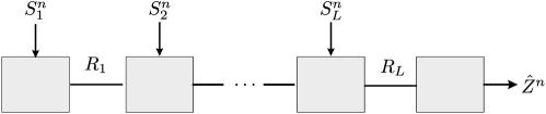
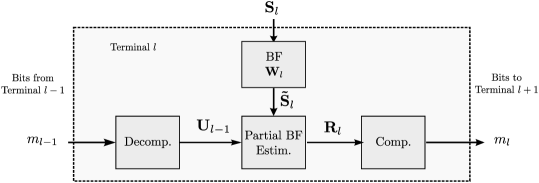
Consider the cascade communication system for function computation shown in Figure 1. Terminal , , observes, or measures, a discrete memoryless source and communicates with Terminal over an error-free finite-capacity link of rate . Terminal does not observe any source, and plays the role of a decoder which wishes to reconstruct a function lossily, to within some average fidelity level , where for some function . The memoryless sources are arbitrary correlated among them, with joint measure . For this communication system, optimal tradeoffs among compression rate tuples and allowed distortion level , captured by the rate-distortion region of the model, are not known in general, even if the sources are independent. For some special cases, inner and outer bounds on the rate-distortion region, that do not agree in general, are known, e.g., in [2] for the case . A related work for the case has also appeared in [3]. For the general case with , although a single-letter characterization of the rate-distortion region seems to be out of reach, one can distinguish essentially two different transmission approaches or modes. In the first mode, each terminal operates essentially as a routing node. That is, each terminal in the cascade sends an appropriate compressed version, or description, of the source that it observes; the decoder reconstructs all sources, lossily, and then computes an estimate of the desired function. In this approach, the computation is performed centrally, at only the decoder, i.e., Terminal . In the second mode, Terminal , , processes the information that it gets from the previous terminal, and then describes it, jointly with its own observation or source, to the next terminal. That is, in a sense, the computation is performed distributively in the network. (See, e.g., [4, 5, 6], where variants of this approach are sometimes referred to as in-network processing).
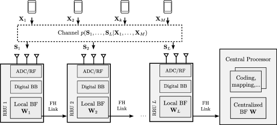
Consider now the seemingly unrelated uplink multiple-input multiple-output (MIMO) system model shown in Figure 2. In this model, users communicate concurrently with a common base station (BS), as in standard uplink wireless systems. The base station is equipped with a large number of antennas, e.g., a Massive MIMO BS; and the baseband processing is distributed across a number, say , of modules or radio remote units (RRUs). The modules are connected each to a small number of antennas; and are concatenated in a line network, through a common fronthaul link that connects them to a central processor (CP) unit. This architecture, sometimes referred to as “chained MIMO” [7] and proposed as an alternative to the standard one in which each RRU has its dedicated fronthaul link to the CP [8, 9, 10, 11, 12, 13, 14, 15, 16, 17], offers a number of advantages and an additional degree of flexibility if more antennas/modules are to be added to the system. The reader may refer to [18, 19, 20, 21] where examples of testbed implementations of this novel architecture can be found. For this architecture, depending on the amount of available channel state information (CSI), receive-beamforming operations may be better performed centrally at the CP or distributively across RRUs. Roughly, if CSI is available only at the CP, not at the RRUs, it seems reasonable that beamforming operations be performed only centrally, at the CP. In this case, RRU , , sends a compressed version of its received signal to the CP which first collects the vector and then performs receive-beamforming on it. In contrast, if local CSI is available or can be acquired at the RRUs, due to the linearity of the receive beamforming (which is a simple matrix multiplication) parts of the receive beamforming operations can be performed distributively at the RRUs (see Section III).
The above shows some connections among the model of Figure 2 and that, more general, of Figure 1. In this paper, we study them using a common framework. Specifically, we develop two coding schemes for the multiterminal cascade source coding problem of Figure 1; and then show that their application to the uplink cascade MIMO system of Figure 1 leads to schemes for receive-beamforming which, depending on the amount of available CSI at the RRUs, are better performed centrally at the CP or distributively across RRUs. In the first coding scheme, each terminal in the cascade sends a description of the source that it observes; the decoder reconstructs all sources lossily and then computes an estimate of the desired function. This scheme improves upon standard routing in that every terminal only compresses the innovation of its source w.r.t. the descriptions that are sent by the previous terminals in the cascade. In the second scheme, the desired function is computed gradually in the cascade network; and each terminal sends a finer description of it. Furthermore, we also derive a lower bound on the minimum distortion at which the desired function can be reconstructed at the decoder by relating the problem to the Wyner-Ziv type system studied in [22]. Numerical results show that the proposed methods outperform standard compression strategies and perform close to the lower bound in some regimes.
I-A Notation
Throughout, we use the following notation. Upper case letters are used to denote random variables, e.g., ; lower case letters used to denote realizations of random variables ; and calligraphic letters denote sets, e.g., . The cardinality of a set is denoted by . The length- sequence is denoted as ; and, for the sub-sequence is denoted as . Boldface upper case letters denote vectors or matrices, e.g., , where context should make the distinction clear. For an integer , we denote the set of integers smaller or equal as ; and, for , we use the shorthand notations , and . We denote the covariance of a vector by ; is the cross-correlation , and the conditional correlation matrix of given as . The length- vector with all entries equal zero but the -th element which is equal unity is denoted as , i.e., ; and the matrix whose entries are all zeros, but the first diagonal elements which are equal unity, is denoted by , for and otherwise. We also, define .
II Cascade Source Coding System Model
Let be a sequence of independent and identically distributed (i.i.d.) samples of the -dimensional source jointly distributed as over . For convenience, we denote .
A cascade of terminals are concatenated as shown in Figure 1, such that Terminal , , is connected to Terminal over an error-free link of capacity bits per channel use. Terminal is interested in reconstructing a sequence lossily, to within some fidelity level, where , , for some function . To this end, Terminal , , which observes the sequence and receives message from Terminal , generates a message as for some encoding function , and forwards it over the error-free link of capacity to Terminal . At Terminal , the message is mapped to an estimate of , using some mapping . Let be the reconstruction alphabet and be a single letter distortion. The distortion between and the reconstruction is defined as .
Definition 1.
A tuple is said to achieve distortion for the cascade multi-terminal source coding problem if there exist encoding functions , , and a function such that
The rate-distortion (RD) region of the cascade multi-terminal source coding problem is defined as the closure of all rate tuples that achieve distortion .
III Schemes for Cascade Source Coding
In this section, we develop two coding schemes for the cascade source coding model of Figure 1 and analyze the RD regions that they achieve.
III-A Improved Routing (IR)
A simple strategy which is inspired by standard routing (SR) in graphical networks and referred to as multiplex-and-forward in [5] has Terminal , , forward a compressed version of its source to the next terminal, in addition to the bit stream received from the previous terminal in the cascade (without processing). The decoder decompresses all sources and then outputs an estimate of the desired function. In SR, observations are compressed independently and correlation with the observation of the next terminal in the cascade is not exploited.
In this section, we propose a scheme, to which we refer to as “Improved Routing” (IR), which improves upon SR by compressing at each terminal its observed signal into a description considering the compressed observations from the previous terminals, i.e., as side information available both at the encoder and the decoder [23]. Thus, each terminal only compresses the innovative part of the observation with respect to the compressed signals from previous terminals (see Section IV-A). In doing so, it uses bits per source sample. Along with the produced compression index of rate , each terminal also forwards the bit stream received from the previous terminal to the next one without processing. The decoder successively decompresses all sources and outputs an estimate of the function of interest.
Theorem 1.
The RD region that is achievable with the IR scheme is given by the union of rate tuples satisfying
| (1) |
for some joint pmf and function , s.t. and .
Remark 1.
The auxiliary random variables that are involved in (1) satisfy the following Markov Chains
| (2) |
where and .∎
Outline Proof: Fix , and a joint pmf that factorizes as
| (3) |
and a reconstruction function such that . Also, fix non-negative such that for , for .
Codebook generation: Let for . Generate a codebook consisting of a collection of codewords , indexed with , where codeword has its elements generated i.i.d. according to . For each index , generate a codebook consisting of a collection of codewords indexed with , where codeword is generated independently and i.i.d. according to . Similarly, for each index tuple generate a codebook of codewords indexed with , and where codeword has its elements generated i.i.d. according to .
Encoding at Terminal 1: Terminal finds an index such that is strongly -jointly typical with , i.e., . Using standard arguments, this step can be seen to have vanishing probability of error as long as is large enough and
| (4) |
Then, it forwards to Terminal 2.
Encoding at Terminal : Upon reception of with the indices , Terminal finds an index such that are strongly -jointly typical with , i.e., . Using standard arguments, this step can be seen to have vanishing probability of error as long as is large enough and
| (5) |
Then, it forwards and to Terminal as .
Reconstruction at end Terminal : Terminal collects all received indices as , and reconstructs the codewords . Then, it reconstructs an estimate of sample-wise as , . Note that in doing so, the average distortion constraint is satisfied.
Remark 2.
In the coding scheme of Theorem 1, the compression rate on the communication hop between Terminal and Terminal , , can be improved further (i.e., reduced) by taking into account sequence as decoder side information, through Wyner-Ziv binning. The resulting strategy, however, is not of “routing type”, unless every Wyner-Ziv code is restricted to account for the worst side information ahead in the cascade, i.e., binning at Terminal accounts for the worst quality side information among the sequences . Also, in this case, since the end Terminal , or CP, does not observe any side information, i.e., , this strategy makes most sense if the Wyner-Ziv codes are chosen such that the last relay terminal in the cascade, i.e., Terminal , recovers an estimate of the desired function and then sends it using a standard rate-distortion code to the CP in a manner that allows the latter to reconstruct the desired function to within the desired fidelity level.
The above routing scheme necessitates that every terminal , , reads the compressed bit streams from previous terminals in the cascade prior to the compression of its own source. This is reflected through treated not only as decoder side information but also as encoder side information. From a practical viewpoint, treating previous terminals streams as encoder side information improves rates but generally entails additional delays. The following corollary specializes the result of Theorem 1 to the case in which is treated only as decoder side information, i.e., the auxiliary random variables are restricted to satisfy that forms a Markov chain. We also present an alternate coding scheme that is based on successive Wyner-Ziv coding [24].
Corollary 1.
The RD region that is achievable with the WZR scheme is given by the set of rate tuples satisfying
| (6) |
for some joint pmf and function s.t. .
Remark 3.
The auxiliary random variables that are involved in (6) satisfy the following Markov Chains
| (7) |
where and . ∎
Outline Proof: The proof of Corollary 1 follows by applying successively standard Wyner-Ziv source coding [24]. Hereafter, we only outline the main steps, for the sake of brevity. Fix and a joint pmf that factorizes as
| (8) |
and a function such that . Also, fix non-negative , such that for for .
Codebook generation: Let non-negative , and set for . Generate codebooks , , with codebook consisting of a collection of independent codewords indexed with , where codeword has its elements generated i.i.d. according to . Randomly and independently assign these codewords into bins indexed with , each containing codewords.
Encoding at Terminal : Terminal finds an index such that is strongly -jointly typical111For formal definitions of strongly -joint typicality, the reader may refer to [23]. with , i.e., . Using standard arguments, it is easy to see that this can be accomplished with vanishing probability of error as long as is large and
| (9) |
Let such that . Terminal then forwards the bin index and the received message to Terminal as .
Reconstruction at the end Terminal : Terminal collects all received bin indices as , and reconstructs the codewords successively in this order, as follows. Assuming that codewords have been reconstructed correctly, it finds the appropriate codeword by looking in the bin for the unique that is -jointly typical with . Using standard arguments, it is easy to see that the error in this step has vanishing probability as long as is large and
| (10) |
Terminal reconstructs an estimate of sample-wise as , . Note that in doing so the average distortion constraint is satisfied.
Finally, substituting and combining (9) and (10), we get (6); and this completes the proof of Corollary 1. ∎
Remark 4.
Remark 5.
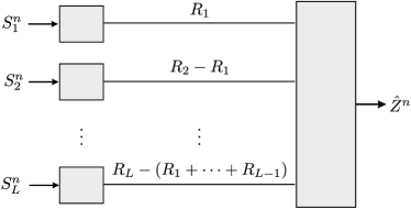
As it can be conveyed from the proof of Corollary 1, since every Terminal , , uses a part of its per-sample rate to simply route the bit streams received from the previous terminals in the cascade and the remaining per-sample bits to convey a description of its observed source , the resulting scheme can be seen as one for the model shown in Figure 3 in which the terminals are connected through parallel links to the CP. Using this connection, the performance of the above WZR scheme can be further improved by compressing the observations à-la Berger-Tung [25].
Remark 6.
In accordance with Remark 2, for the model of Figure 1 yet another natural coding strategy is one in which one decomposes the problem into successive Wyner-Ziv type problems for function computation, one for each hop. Specifically, in this strategy one sees the communication between Terminal and Terminal , , as a Wyner-Ziv source coding problem with two-sided state information, state information at the encoder and state information at the decoder. This strategy, which is not of “routing type”, is developed in the next section.
III-B In-Network Processing (IP)
In the routing schemes in Section III-A, the function of interest is computed at the destination from the compressed observations, i.e., the terminals have to share the fronthaul to send a compressed version of their observations to Terminal . We present a scheme to which we refer to as “In-Network Processing” (IP), in which instead, each terminal computes a part of the function to reconstruct at the decoder so that the function of interest is computed along the cascade. To that end, each terminal decompresses the signal received from the previous terminal and jointly compresses it with its observation to generate an estimate of the part of the function of interest, which is forwarded to the next terminal (see Section IV-C). Correlation between the computed part of the function and the source at the next terminal is exploited through Wyner-Ziv coding. Note that by decompressing and recompressing the observations at each terminal, additional distortion is introduced [2].
Theorem 2.
The RD region that is achievable with IP is given by the union of rate tuples satisfying
| (11) |
for some joint pmf and a function , such that and .
Remark 7.
The auxiliary random variables that are involved in (11) satisfy the following Markov Chains
| (12) |
where , . ∎
Outline Proof: Fix and a joint pmf that factorizes as
| (13) |
and a function such that . Also fix non-negative .
Codebook generation: Let non-negative . Generate codebooks , , with codebook consisting of a collection of independent codewords , indexed with , where codeword has its elements generated randomly and independently i.i.d. according to . Randomly and independently assign these codewords into bins indexed with , each containing codewords.
Encoding at Terminal : Terminal finds an index such that is strongly -jointly typical with , i.e., . Using standard arguments, it is easy to see that this can be accomplished with vanishing probability of error as long as is large and
| (14) |
Let such that . Terminal then forwards the index to Terminal .
Decompression and encoding at Terminal : Upon reception of the bin index from Terminal , Terminal finds by looking in the bin for the the unique that is -jointly typical with . Using standard arguments, it can be seen that this can be accomplished with vanishing probability of error as long as is large enough and
| (15) |
Then, Terminal finds an index such that is strongly -jointly typical with , i.e., . Using standard arguments, it can be seen that this can be accomplished with vanishing probability of error as long as is large and
| (16) |
Let such that . Terminal forwards the bin index to Terminal as . Reconstruction at end Terminal : Terminal collects the bin index and reconstructs the codeword by looking in the bin . Since Terminal does not have available any side information sequence, from (15), successful recovery of the unique in the bin requires . That is, each bin contains a single codeword and . Then, Terminal reconstructs an estimate of sample-wise as , . In doing so, the average distortion constraint is satisfied.
Remark 8.
It is shown in [2] that for , in general none of the IR and IP schemes outperform the other; and a scheme combining the two strategies is proposed.
IV Centralized and Distributed Beamforming in Chained MIMO Systems
In this section, we apply the cascade source coding model to study the achievable distortion in a Gaussian uplink MIMO system with a chained MIMO architecture (C-MIMO) in which single antenna users transmit over a Gaussian channel to RRUs as shown in Figure 2. The signal received at RRU , , equipped with antennas, , is given by
| (17) |
where is the signal transmitted by the users and , is the signal transmitted by user . We assume that each user satisfies an average power constraint , , where ; is the channel between the users and RRU and is the additive ambient noise.
The transmitted signal by the users is assumed to be distributed as and we denote the observations at the RRUs as . Thus, we have , where and .
In traditional receive-beamforming, a beamforming filter is applied at the decoder on the received signal to estimate the channel input with the linear function
| (18) |
In C-MIMO, the decoder (the CP) is interested in computing the receive beamforming signal with minimum distortion, although is not directly available at the CP but remotely observed at the terminals. Depending on the available CSI, receive-beamforming computation may be better performed centrally at the CP or distributively across the RRUs:
Centralized Beamforming: If CSI is available only at the CP, not at the RRUs, it seems reasonable that beamforming operations are performed only centrally at the CP. In this case, RRU , , sends a compressed version of its output signal to the CP, which first collects the vector , and then performs receive-beamforming on it.
Distributed Beamforming: If local CSI is available at the RRUs, or can be acquired, receive beamforming operations can be performed distributively along the cascade. Due to linearity the joint beamforming operation (18) can be expressed as a function of the received source as
| (19) |
where corresponds to blocks of columns of such that . In this case, the receive beamforming signal can be computed gradually in the cascade network, by letting the RRUs compute a part of the desired function, e.g., as proposed in Section IV-C, RRU , computes an estimate of .
The distortion between and the reconstruction of the beamforming signal at the CP is measured with the sum-distortion
| (20) |
For a given fronthaul tuple in the RD region , the minimum achievable average distortion is characterized by the distortion-rate function222This formulation is equivalent to the rate-distortion framework considered in Section III; here we consider the distortion-rate formulation for convenience. given by
| (21) |
Next, we study the distortion-rate function in a Gaussian C-MIMO model under centralized and distributed beamforming with the schemes proposed for the cascade source coding problem.
IV-A Centralized Beamforming with Improved Routing
In this section, we consider distortion-rate function of the IR scheme in Section III-A applied for centralized beamforming. Each RRU forwards a compressed version of the observation to the CP, which estimates the receive-beamforming signal from the decompressed observations. While the optimal test channels are in general unknown, next theorem gives the distortion-rate function of IR for centralized beamforming for the C-MIMO setup under jointly distributed Gaussian test channels.
Theorem 3.
The distortion-rate function for the IR scheme under jointly Gaussian test channels is given by
| (22) | ||||
| (23) | ||||
| (24) |
where and , , , , .
Proof: We evaluate Theorem 1 by considering jointly Gaussian sources and test channels satisfying and the minimum mean square error (MMSE) estimator as reconstruction function , where we define and . Note that MMSE reconstruction is optimal under (20), while considering jointly Gaussian test channels might be suboptimal in general. First we derive a lower bound on the achievable distortion. We have
| (25) | ||||
| (26) | ||||
| (27) | ||||
| (28) |
where in (26) we define the MMSE error , which is Gaussian distributed as ; (27) follows due to the orthogonality principle [23], and due to the fact that for Gaussian random variables, orthogonality implies independence of and .
For the fixed test channels, let us choose matrix such that for
| (29) |
Note that such always exists since , and can be found explicitly as follows. After some straightforward algebraic manipulations, (29) can be written as , where . Note that , and let and . Then, it follows that is given by , where and . Then, from (28), we have
| (30) | ||||
| (31) | ||||
| (32) |
The distortion is lower bounded as
| (33) |
where (33) follows due to the linearity of the MMSE estimator for jointly Gaussian variables.
The lower bound given by (32) and (33) is achievable by letting , with , and independent of all other variables, as follows
| (34) | ||||
| (35) | ||||
| (36) | ||||
| (37) | ||||
| (38) |
where (36) follows since and (37) is due to the orthogonality principle. In the case , we have which can be trivially achieved by letting .
Optimizing over the positive semidefinite covariance matrices gives the desired minimum distortion in Theorem 3. This completes the proof. ∎
The IR scheme in Section III-A requires joint compression at RRU of the observed source and the previous compression codewords to generate the compression codeword . However, for the Gaussian C-MIMO, it is shown next that the sum-distortion in Theorem 3 can also be achieved by applying at each RRU separate decompression of the previous compression codewords, the innovation sequence computation , followed by independent compression of into a codeword , which is independent of the previous compression codewords , as follows. See Figure 5. At RRU :
-
•
Upon receiving bits , decompress .
-
•
Compute the innovation sequence .
-
•
Compress at bits per sample independently of using a codeword , where , with independent of each other.
Note that corresponds to the MMSE error of estimating from , and is an i.i.d. zero-mean Gaussian sequence distributed as .
Proposition 1.
For the Gaussian C-MIMO model, separate decompression, innovation computation and independent innovation compression achieves the minimum distortion characterized by the distortion-rate function in Theorem 3.
Proof: We show that any distortion achievable for a pmf and the corresponding in Theorem 3 is also achievable with separate decompression, innovation computation and compression as detailed above. From standard arguments, compressing at bits requires
| (39) | ||||
| (40) | ||||
| (41) |
where (41) follows since , which follows since RRU can compute for , which is distributed as the test channels and thus .
The distortion between and its estimation from satisfies
| (42) | ||||
| (43) | ||||
| (44) |
Thus, any achievable distortion for given and fixed in Theorem 3 is achievable by separate decompression, innovation computation and independent compression of the innovation. This completes the proof. ∎
Determining the optimal covariance matrices achieving in Theorem 3 requires a joint optimization, which is generally not simple. Next, we propose a method to successively obtain a feasible solution and the corresponding minimum distortion for given :
-
1.
For a given fronthaul tuple , fix non-negative , satisfying , for .
-
2.
For such , sequentially find from RRU to RRU as the minimizing the distortion between the innovation and its reconstruction as follows. At RRU , for given and , is found from the covariance matrix minimizing
(45) Note that (45) corresponds to the distortion-rate problem of compressing a Gaussian vector source at bits and its solution is given below in Proposition 2.
-
3.
Compute the achievable distortion by evaluating as in Theorem 1 with the chosen covariance matrices .
-
4.
Compute as the minimum over satisfying the fronthaul constraints for .
The solution for the distortion-rate problem in (45) is standard and given next for completeness.
Proposition 2.
Given , let , where and . The optimal distortion (45) is where is the solution to
| (46) |
and is achieved with , where and 333Note the slight abuse of notation. If for the -th uncorrelated components we have , in the achievability we have . It should be understood that the -th component is not assigned any bit for compression. This is in line with (46) as the number of bits assigned for the -th component is given by ..
Outline Proof: The minimization of the RD problem in (45) is standard, e.g. [26], and well known to be achieved by uncorrelating the vector source into uncorrelated components as . Then, the available bits are distributed over the parallel source components by solving the reverse water-filling problem
The solution to this problem is given by , where satisfies (46). The optimality of follows since is achieved with as stated in Proposition 2 [26, 27]. ∎
IV-B Centralized Beamforming with Successive Wyner-Ziv
In this section, we consider the distortion-rate function of the WZR scheme in Corollary 1 for centralized beamforming. Similarly to IR, each RRU forwards a compressed version of its observation to the CP, which estimates the receive-beamforming signal from the decompressed observations. Next theorem shows that WZR achieves the same distortion-rate function as the IR scheme under jointly Gaussian test channels.
Theorem 4.
The distortion-rate function of the WZR scheme with jointly Gaussian test channels, is the same as the distortion-rate function of the IR scheme with Gaussian test channels in Theorem 3, i.e.,
Outline Proof: Since , we only need to show that any distortion achievable with IR in Theorem 3 is also achievable with WZR. For fixed and with IR in Theorem 3, the minimum distortion is achieved by considering a test channel . Since this test channel is also in the class of test channels of WZR, it follows that any achievable distortion for fixed and in Theorem 3 is achievable with WZR. ∎
IV-C In-Network Processing for Distributed Beamforming
In this section, we study the distortion-rate function of the IP scheme in Section III-B for distributed beamforming. At each RRU, the received signal from the previous terminal is jointly compressed with the observation and forwarded to the next RRU. While the optimal joint compression per RRU along the cascade remains an open problem, even for independent observations [23], we propose to gradually compute the desired function by reconstructing at each RRU parts of . In particular, compression at RRU is designed such that RRU reconstructs from and the received bits an estimate of the part of the function:
| (47) |
The design of the compression is done successively. Assuming are fixed, at RRU , , is obtained as the solution to the following distortion-rate problem:
| (48) | ||||
| (49) |
Problem (48)-(49) corresponds to the distortion-rate function of the Wyner-Ziv type source coding problem of lossy reconstruction of function as , which is a function of the encoder observation when side information , is available at the decoder [22]. Proposition 3 given below characterizes the optimal test channel at RRU given , i.e., , and shows that it is Gaussian distributed as,
| (50) |
where and .
Remark 9.
Remark 10.
Equation (52) highlights that due to the successive decompression and recompression performed at each RRU, the quantization noises propagate throughout the cascade. The linear combination of the locally beamformed signal and the decompressed signal can be seen as a noisy observation of the remote sources , through an additive channel with channel coefficients and correlated noise . This noisy signal is used as an estimate of the partial beamformed signal (47) to be reconstructed at the next RRU.
Next proposition characterizes the optimal test channel in (50) with and for given test channels with their corresponding and .
Proposition 3.
Let , , where and , and , where . The minimum distortion (48) is and satisfies
| (53) |
where , , , In addition, the minimum distortion in is achieved with and , where is a diagonal matrix, with the -th diagonal element .
Outline Proof: The proof is similar to that of the remote Wyner-Ziv source coding problem for source reconstruction in [27]. We consider lossy function reconstruction. For simplicity, we drop the RRU index in this proof and define , , and .
First, we obtain a lower bound on the achievable distortion. Let us define the MMSE filters
| (56) |
We have from the MMSE estimation of Gaussian vector sources [23],
| (57) | ||||
| (58) |
where and correspond to the MMSE errors and are zero-mean jointly Gaussian random vectors independent of each other, is independent of and is independent of and have the covariance matrices given by and .
On the other distortion side, we have
| (59) | ||||
| (60) | ||||
| (61) | ||||
| (62) |
where (61) follows from (58) and where we have defined ; (62) follows from the independence of from , and .
Next, let us define and , where follows from the eigenvalue decomposition
| (63) |
Note that has independent components of variance . Therefore, from (62) we have
| (64) | ||||
| (65) |
where (64) follows due to the orthonormality of .
On the other hand, we have
| (66) | ||||
| (67) | ||||
| (68) | ||||
| (69) | ||||
| (70) | ||||
| (71) | ||||
| (72) | ||||
| (73) |
where (67) follows due to the data processing inequality; (69) is due to (57) and the orthogonality principle of the MMSE estimator; (70) is due to the definition of ; (71) follows since conditioning reduces entropy; and (73) is due to the data processing inequality and since , where , is a function of .
It follows from (65) and (73) that is lower bounded by the sum-distortion of compressing , , given as a reverse water filling problem with a modified distortion , so that is reconstructed with distortion ,
| (74) |
Note that if , then and if , then . The minimum is found with , for satisfying (53) [26].
The achievability of the derived lower bound follows by considering the set of tuples in in Theorem 2 for satisfying the additional Markov chain , which is included in , as , with and and where and . ∎
The distortion-rate function of the proposed IP scheme in Gaussian C-MIMO is given next.
Theorem 5.
Given with and successively obtained as in Proposition 3, the distortion-rate of the proposed IP scheme function is given as
| (75) |
where ; ; , and .
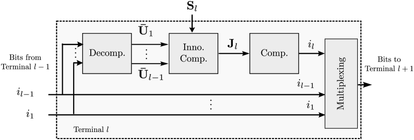
The IP scheme in Section III-B requires joint compression at each RRU. However, for the Gaussian C-MIMO, it is shown next that the distortion-rate function in Theorem 5 can be achieved by applying at each RRU separate decompression, partial function estimation followed by compression, as shown in Figure 6. At RRU :
-
•
Upon receiving , decompress .
-
•
Apply local beamforming as .
-
•
Linearly combine , to compute an estimate of the partial function up to Terminal :
(76) -
•
Forward a compressed version of to Terminal using Wyner-Ziv compression considering as side information and the test channel , .
Terminal reconstructs using an MMSE estimator as .
Proposition 4.
For the C-MIMO model, separate decompression, partial function estimation and Wyner-Ziv compression achieves the distortion-rate function in Theorem 5.
Proof: The proof follows by showing that at any RRU , the minimum distortion and the test channel in Proposition 3 can also be obtained with separate decompression, partial function estimation and compression. RRU decompresses and computes and . From standard arguments, it follows that compressing à-la Wyner-Ziv with as decoder side information requires
| (77) | ||||
| (78) | ||||
| (79) |
where (78) follows since is orthonormal.
V A Lower Bound
In this section, we obtain an outer bound on the RD region using a Wyner-Ziv type system in which the decoder is required to estimate the value of some function of the input at the encoder and the side information [22]. We use the following notation from [28]. Define the minimum average distortion for given as , and the Wyner-Ziv type RD function for value , encoder input and side information available at the decoder, as [22]
| (80) |
An outer bound can be obtained using the rate-distortion Wyner-Ziv type function in (80).
Theorem 6.
The RD region is contained in the region , given by the union of tuples satisfying
| (81) |
Outline Proof: The outer bound is obtained by the RD region of network cuts, such that for the -th cut, acts as side information at the decoder. See Appendix A. ∎
In the Gaussian C-MIMO model, Theorem 6 can be used to explicitly write a lower bound on the achievable distortion for a given fronthaul tuple as given next.
Proposition 5.
Given the fronthaul tuple , the achievable distortion in a C-MIMO system is lower bounded by , where
| (82) |
with , for and are the eigenvalues of , with .
VI Numerical Results
In this section, we provide numerical examples to illustrate the average sum-distortion obtained using IR and IP as detailed in Section IV. We consider several C-MIMO examples, with users and RRUs, each equipped with antennas under different fronthaul capacities. The CP wants to reconstruct the receive-beamforming signal using the Zero-Forcing weights given by
| (83) |
The channel coefficients are distributed as . We also consider the SR scheme of [5]. The schemes are compared among them, and to the lower bound in Theorem 6. Note that WZR achieves the same distortion-rate function as IR as shown in Theorem 4, and is omitted.
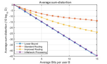
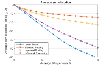
Figure 8 depicts the sum-distortion in a C-MIMO network with users and RRUs, each equipped with antennas for equal fronthaul capacity per link , as a function of the average number of bits per user . As it can be seen from the figure, the scheme IP based on distributed beamforming outperforms the other centralized beamforming schemes, and performs close to the lower bound. For centralized beamforming, the scheme IF performs significantly better than SR, as it reduces the required fronthaul by only compressing the innovation at each RRU.
Figure 8 shows the sum-distortion in a C-MIMO network with users and RRUs, each equipped with antennas, with increasing fronthaul capacity per link , as a function of the average number of bits per user . In this case, the IP scheme using distributed beamforming also achieves the lowest sum-distortion among the proposed schemes.
References
- [1] I. Estella and A. Zaidi, “In-network compression for multiterminal cascade mimo systems,” in to appear in Proc. IEEE Int’l Conference on Communications (ICC), Paris, France, May 2017.
- [2] P. Cuff, H. I. Su, and A. E. Gamal, “Cascade multiterminal source coding,” in Proc. IEEE Int’l Symposium on Information Theory Proceedings (ISIT), Jun. 2009, pp. 1199–1203.
- [3] H. Permuter and T. Weissman, “Cascade and triangular source coding with side information at the first two nodes,” IEEE Tran. Inf. Theory, vol. 58, no. 6, pp. 3339–3349, Jun. 2012.
- [4] M. Sefidgaran and A. Tchamkerten, “Distributed function computation over a rooted directed tree,” IEEE Tran. Inf. Theory, vol. PP, no. 99, pp. 1–1, Feb. 2016.
- [5] S. H. Park, O. Simeone, O. Sahin, and S. Shamai, “Multihop backhaul compression for the uplink of cloud radio access networks,” IEEE Trans. on Vehic. Tech., vol. PP, no. 99, pp. 1–1, May 2015.
- [6] Y. Yang, P. Grover, and S. Kar, “Coding for lossy function computation: Analyzing sequential function computation with distortion accumulation,” in IEEE Int’l Symposium on Information Theory (ISIT), Jul. 2016, pp. 140–144.
- [7] A. Puglielli, N. Narevsky, P. Lu, T. Courtade, G. Wright, B. Nikolic, and E. Alon, “A scalable massive MIMO array architecture based on common modules,” in 2015 IEEE Int’l Conference on Communication Workshop (ICCW), Jun. 2015, pp. 1310–1315.
- [8] O. Somekh, B. Zaidel, and S. Shamai, “Sum rate characterization of joint multiple cell-site processing,” IEEE Trans. Inf. Theory, vol. 53, no. 12, pp. 4473–4497, Dec. 2007.
- [9] A. Del Coso and S. Simoens, “Distributed compression for MIMO coordinated networks with a backhaul constraint,” IEEE Trans. Wireless Comm., vol. 8, no. 9, pp. 4698–4709, Sep. 2009.
- [10] A. Sanderovich, O. Somekh, H. Poor, and S. Shamai, “Uplink macro diversity of limited backhaul cellular network,” IEEE Trans. Inf. Theory, vol. 55, no. 8, pp. 3457–3478, Aug. 2009.
- [11] S.-H. Park, O. Simeone, O. Sahin, and S. Shamai, “Robust and efficient distributed compression for cloud radio access networks,” IEEE Trans. Vehicular Technology, vol. 62, no. 2, pp. 692–703, Feb. 2013.
- [12] ——, “Joint decompression and decoding for cloud radio access networks,” IEEE Signal Processing Letters, vol. 20, no. 5, pp. 503–506, May 2013.
- [13] Y. Zhou and W. Yu, “Optimized backhaul compression for uplink cloud radio access network,” IEEE Journal on Sel. Areas in Comm., vol. 32, no. 6, pp. 1295–1307, Jun. 2014.
- [14] B. Nazer, A. Sanderovich, M. Gastpar, and S. Shamai, “Structured superposition for backhaul constrained cellular uplink,” in Proc. IEEE Int’l Symposium on Information Theory (ISIT), Seoul, Korea, Jun. 2012.
- [15] S.-N. Hong and G. Caire, “Compute-and-forward strategies for cooperative distributed antenna systems,” IEEE Trans. Inf. Theory, vol. 59, no. 9, pp. 5227–5243, Sep. 2013.
- [16] I. Estella-Aguerri and A. Zaidi, “Lossy compression for compute-and-forward in limited backhaul uplink multicell processing,” IEEE Trans. Communications, vol. 64, no. 12, pp. 5227–5238, Dec. 2016.
- [17] I. Estella and A. Zaidi, “Partial compute-compress-and-forward for limited backhaul uplink multicell processing,” in Proc. 53rd Annual Allerton Conf. on Comm., Control, and Computing, Monticello, IL, Sep. 2015.
- [18] C. Shepard, H. Yu, N. Anand, E. Li, T. Marzetta, R. Yang, and L. Zhong, “Argos: Practical many-antenna base stations,” in Proc. of the 18th Annual Int’l Conference on Mobile Computing and Networking (Mobicom ’12), 2012, pp. 53–64.
- [19] C. Shepard, H. Yu, and L. Zhong, “ArgosV2: a flexible many-antenna research platform,” in Proc. of the 19th Annual International Conference on Mobile Computing and Networking (MobiCom ’13). New York, NY, USA: ACM, Sep. 2013, pp. 163–166.
- [20] J. Vieira, S. Malkowsky, K. Nieman, Z. Miers, N. Kundargi, L. Liu, I. Wong, V. Öwall, O. Edfors, and F. Tufvesson, “A flexible 100-antenna testbed for massive MIMO,” in 2014 IEEE Globecom Workshops (GC Wkshps), Dec. 2014, pp. 287–293.
- [21] H. V. Balan, M. Segura, S. Deora, A. Michaloliakos, R. Rogalin, K. Psounis, and G. Caire, “USC SDR, an easy-to-program, high data rate, real time software radio platform,” in Proc. of the Second Workshop on Software Radio Implementation Forum (SRIF ’13), Aug. 2013, pp. 25–30.
- [22] H. Yamamoto, “Wyner - Ziv theory for a general function of the correlated sources (corresp.),” IEEE Tran. Inf. Theory, vol. 28, no. 5, pp. 803–807, Sep 1982.
- [23] A. E. Gamal and Y.-H. Kim, Network Information Theory. Cambridge University Press, 2011.
- [24] A. D. Wyner and J. Ziv, “The rate-distortion function for source coding with side information at the decoder,” IEEE Trans. Inf. Theory, vol. 22, pp. 1–10, Jan. 1976.
- [25] T. Berger and R. Yeung, “Multiterminal source encoding with one distortion criterion,” IEEE Trans. Inf. Theory, vol. 35, no. 2, pp. 228–236, Mar. 1989.
- [26] T. M. Cover and J. A. Thomas, Elements of Information Theory. Wiley-Interscience, 1991.
- [27] C. Tian and J. Chen, “Remote vector Gaussian source coding with decoder side information under mutual information and distortion constraints,” IEEE Tran. Inf. Theory, vol. 55, no. 10, pp. 4676–4680, Oct. 2009.
- [28] S. Shamai, S. Verdú, and R. Zamir, “Systematic lossy source-channel coding,” IEEE Trans. Inf. Theory, vol. 44, no. 2, pp. 564–579, Mar. 1998.
Appendix A Proof of Theorem 6
Suppose there exist , and such that for , , where as . Define for , where and note the Markov chain relation
| (84) |
For the -th cut we have,
| (85) | ||||
| (86) | ||||
| (87) | ||||
| (88) | ||||
| (89) | ||||
| (90) |
where (87) follows since is i.i.d., (88) follows since conditioning reduces entropy. On the other hand, we have
| (91) | ||||
| (92) | ||||
| (93) |
where (92) follows since is a deterministic function of , i.e., , (93) follows since reducing the information can only increase the distortion, Then,
| (94) | ||||
| (95) | ||||
| (96) |
where (94) follows since is monotonic in , (95) is due to being a function of , and (96) follows as is convex and monotone in . This completes the proof.∎