Polydisperse polymer brushes: internal structure, critical behavior, and interaction with flow

Abstract

ABSTRACT: We study the effect of polydispersity on the structure of polymer brushes by analytical theory, a numerical self-consistent field approach, and Monte Carlo simulations. The polydispersity is represented by the Schulz-Zimm chain-length distribution. We specifically focus on three different polydispersities representing sharp, moderate and extremely wide chain length distributions and derive explicit analytical expressions for the chain end distributions in these brushes. The results are in very good agreement with numerical data obtained with self-consistent field calculations and Monte Carlo simulations. With increasing polydispersity, the brush density profile changes from convex to concave, and for given average chain length $N_{n}$ and grafting density $\sigma$, the brush height $H$ is found to scale as $(H/H_{\mathrm{mono}}-1)\propto(\mbox{${N_{w}}/{N_{n}}$}-1)^{1/2}$ over a wide range of polydispersity indices ${N_{w}}/{N_{n}}$ (here $H_{\mathrm{mono}}$ is the height of the corresponding monodisperse brush. Chain end fluctuations are found to be strongly suppressed already at very small polydispersity. Based on this observation, we introduce the concept of the brush as a near-critical system with two parameters (scaling variables), $(N_{n}\sigma^{2/3})^{-1}$ and $(N_{w}/N_{n}-1)^{1/2}$, controlling the distance from the critical point. This approach provides a good description of the simulation data. Finally we study the hydrodynamic penetration length $l_{\mathrm{p}}$ for brush-coated surfaces in flow. We find that it generally increases with polydispersity. The scaling behavior crosses over from $l_{\mathrm{p}}\sim N_{\mathrm{n}}^{1/2}\sigma^{-1/6}$ for monodisperse and weakly polydisperse brushes to $l_{\mathrm{p}}\sim N_{n}^{2/3}$ for strongly polydisperse brushes.

I Introduction

Polymer brushes have been the subject of intense investigations starting from the seminal paper by Alexander roughly 40 years ago Alexander:1977 . As surface modifiers, they have applications in various fields, e.g., as anti-fouling surfaces Biofouling , lubrication Klein:1991 ; Singh:2015 , biomedicine Zdyrko:2009 , biomaterial Ayres:2010 , nanosensoring Stimuli_responsive ; Cohen_Stuart and others. The current level of understanding of brushes is to a large extent based on a relatively simple but detailed analytical theory, which was proposed at an early stage MWC ; Zhulina ; Skvortsov:1988 . Although the original theory described only equilibrium properties of monodisperse brushes, it gave an impetus for a large body of experimental and simulation-based work extending well outside this scope (see the reviews Klein:1991 ; Advincula:2011 ; Binder_Kreer:2011 ; Halperin:1992 ). As far as the brush density profiles and detailed characteristics of brush-forming chains are concerned, the picture provided by theory and simulations for various chain lengths, grafting densities and solvent qualities is extremely detailed. Thermodynamic parameters such as the chemical potential and the osmotic pressure profiles are also readily available Romeis:2012 ; Netz:2006 ; Netz:1998 .

The experimental synthesis of monodisperse brushes (or brushes with a very narrow molar mass distribution) requires special methods. Polymer brushes formed by long chains are typically produced using “grafting to” and “grafting from” techniques. In the “grafting to” technique, narrowly fractioned pre-formed polymer chains of a given number-averaged chain length $N_{n}$ are tethered to a surface either by chemical bonding or by strong adsorption of a short sticky block. The number of grafted chains per unit area, $\sigma$, can be calculated from the total mass of grafted material and the total area, both directly measurable in the experiment. During the brush synthesis, polymer molecules must diffuse through an existing grafted polymer layer to reach the reactive sites decorating the surface. Due to steric hindrance, this becomes increasingly difficult with increasing height and density of the polymer brush. Hence only synthesize brushes with relatively low grafting densities and moderate brush thickness can be synthesized with this technique. Very recently, it was reported in the literature Minko2016 that the highest grafting density for poly(ethylene glycol) (PEG) brushes that would be obtained using the grafting to method is close to 1.2 chains/nm².

The “grafting from” approach has become the preferred option for the synthesis of dense polymer brushes. This approach uses a surface immobilized initiator layer and subsequent in situ polymerization to generate the polymer brush. The method gives a polydisperse brush with higher grafting density $\sigma$ independent of the polymerization time. In contrast to the “grafting to” methodology, calculating $\sigma$ for systems prepared by the “grafting from” approach is more challenging because $N_{n}$ is unknown a priori. One method of characterizing the chain length distribution (or the molecular weight distribution) is to degraft the polymer chains from a large surface area and collect a sufficient amount of material, which is then analyzed using a sensitive analytical method of size exclusion chromatography. It was shown Turgman that the chain length distribution of the degrafted chains of poly(methyl-methacrylate) is close to the so-called Schulz-Zimm distribution. The values of the polydispersity index, $\mbox{${N_{w}}/{N_{n}}$}\thickapprox 1.15-1.19$, were marginally higher than those typically observed for bulk polymers grown under similar conditions and did not reveal any significant dependence on the polymerization time. (Here $N_{w}$ denotes the weight averaged chain length which can be determined experimentally, e.g., by scattering methods). Thus the experimental techniques available for producing polymer brushes with high polymerization index typically yield rather broad chain length distributions. Broad distributions are also typical for biological brushes covering the surface of some cells or blood vessels Pandav .

It is common wisdom that polydispersity may significantly affect the properties of polymeric systems. However, experimental work comparing the properties of polymer brushes that differ only in polydispersity is still very rare. In Ref. Balko:2013 , curves showing the energy vs. separation upon bringing together two brush-coated surfaces were compared for brushes with $\mbox{${N_{w}}/{N_{n}}$}\thickapprox 1.06$ and $\mbox{${N_{w}}/{N_{n}}$}\thickapprox 1.23$, and similar values for the number-averaged molar mass $M_{n}=37000$ and the grafting density $\sigma=0.195$. Russell and co-workers Russel:2007 observed that surfaces with a quaternary ammonia-modified dry polydisperse brush could kill bacteria cells, while a polymer brush of the same thickness but with low polydispersity could not penetrate the bacterial cell envelope (the charge density is a critical parameter for the killing efficacy).

Polydispersity should also affect the penetration of polymer brushes by proteins. In particular, differences in the fouling properties of brushes were attributed to indirect polydispersity effects although no clear-cut experimental evidence was given Krishnamoorthy:2014 .

From a theoretical point of view, the study of polydispersity effects on the structure and properties of brushes is quite difficult. A general approach based on the self-consistent field (SCF) theory in the strong-stretching limit was proposed by Milner, Witten, and Cates (MWC) Milner_Polydisp . It allows to calculate the brush density profile as well as individual chain stretching characteristics numerically for a given chain length distribution. Closed-form analytical expressions for the density profiles are typically not available, although some global brush characteristics are given in a simple integral form. Intriguingly, almost none of the predictions have been compared to numerical SCF work or simulations. At least part of the problem seems to be psychological, since the variety of conceivable chain length distribution functions is overwhelming. Whether the strong stretching approximation which proved to be so useful in the case of monodisperse brushes is practical for broad chain length distributions remains an open question. Monte Carlo (MC) simulations of polydisperse brushes face the additional challenge that one must perform quenched disorder averages, due to the fact that chains of different length are permanently grafted to a substrate. An extensive numerical SCF study of polydispersity effects on the brush structure was presented in Leermakers on the basis of the Schulz-Zimm distribution, which is commonly used to describe experimental samples. With this choice of distribution shape, the polydispersity parameter ${N_{w}}/{N_{n}}$ can be tuned in a range from 1 to 2. Brush density profiles for moderate grafting density and good solvent conditions were calculated, allowing to study systematic changes in the brush height and in the profile shape with increasing polydispersity. Qualitatively, the picture can be summarized as follows: Starting from the familiar parabolic (convex cap-like) profile in the purely monodisperse case, the mean curvature of the profile decreases monotonically, resulting in clearly concave shapes at $\mbox{${N_{w}}/{N_{n}}$}>1.4$. In the case of moderate polydispersity, $\mbox{${N_{w}}/{N_{n}}$}\simeq 1.15$, the density profile is almost linear. Another paper by the same group addressed the polydispersity effects on the brush penetration by nanoparticles using SCF calculations deVos_nanopartcle . It was shown that the larger the polydispersity, the easier it is for a small particle to penetrate the brush and to touch the substrate. For very large particles an opposite effect is found: it is harder to compress a polydisperse brush than a corresponding monodisperse brush.

In the present paper we study three cases representing vanishingly small, moderate and large polydispersity. By combining closed-form analytical solutions based on the MWC theory with a Green’s function approach we calculate the density profiles and the individual chain conformations (including the chain fluctuations neglected by the strong stretching approximation) and test the theory predictions by MC simulations and one-dimensional SCF numerics. Finally, we examine the effect of polydisperse brushes on hydrodynamical shear flow and calculate in particular the hydrodynamic penetration depth.

The remainder of the paper is organized as follows: Sec. II describes the model system, the MC scheme, and the Schulz-Zimm distribution. In Sec. III, we discuss general characteristics of polydisperse brushes, such as their height and their density profiles. In Sec. IV, we briefly summarize the main predictions of the analytical theory (which are derived in detail in Appendix B, based on the MWC theory). The theoretical predictions are compared with MC simulations and numerical SCF calculations in Sec. V. In this context, we also analyze the chain end fluctuations in weakly polydisperse brushes and introduce the concept of monodisperse brushes as near-critical systems. The implications for the interaction with hydrodynamic flows are discussed in Sec. VI. We close with a summary of the main features of polydisperse brushes in Sec. VII. The Appendix summarizes technical details on the SCF theory and presents the derivations of analytical results – in particular, the analytical expressions for the Green’s function of single chains embedded in three types of brush (monodisperse, moderately polydisperse with exactly linear density profile, and strongly polydisperse) and the expressions for the hydrodynamic penetration length in these brushes.

II Model and Monte Carlo scheme

The system is composed of a dense polydisperse brush in implicit solvent in a volume $V=L_{x}\cdot L_{y}\cdot L_{z}$. We adopt periodic boundaries along the $x$ and $y$ directions, while impenetrable boundary walls are placed $z=0$ and $z=L_{z}$. Polymer chains are modelled as chains of beads connected by harmonic springs with the spring constant $3k_{\mathrm{B}}T/2a^{2}$, where $a$ is the statistical bond length, $k_{B}$ is the Boltzmann constant, and $T$ the temperature. We will use $a$ as the unit length and $k_{B}T$ as the energy unit. Brush chains in the system are grafted with one end each onto a flat substrate located at $z_{0}$, which is chosen $0<z_{0}<a$ for practical reasons. The nonbonded interaction is formulated in terms of the local monomer density, implying that we have soft interactions. The Hamiltonian thus has the Edwards type EdwardsType1 ; EdwardsType2 ; EdwardsType3 ; Hybrid_PF ; Klushin:2015 and can be written as

$$\beta\mathcal{H} = \frac{3}{2a^{2}}\sum_{\alpha=1}^{n_{b}}\sum_{j=1}^{N_{j}-1}\Big{(}\mathbf{R}_{\alpha j}-\mathbf{R}_{\alpha,j-1}\Big{)}^{2}$$ (1)

$$+\frac{v}{2}\int d\mathbf{r}\hat{\phi}^{2}(\mathbf{r})$$

where $\beta\equiv 1/k_{B}T$, and the bond length $a$ is assumed to be the same for each monomer. In the first term $\mathbf{R}_{\alpha j}$ denotes the location of the $j$th bead in the $\alpha$-th chain, the index $\alpha$ running over all $n_{b}$ brush chains, and $N_{\alpha}$ is the chain length for the $\alpha$-th brush chain. The second term represents the nonbonded effective monomer-monomer interactions. Here, $v$ is the excluded volume interaction parameter measuring the monomer-monomer interaction strength in good solvent. The microscopic density of monomers is a function of conformation, $\hat{\phi}=\sum_{\alpha=1}^{n_{b}}\sum_{j}\delta(\mathbf{r}-\mathbf{R}_{\alpha j})$. We will use $\phi$ to denote the smoothed density, for example, the ensemble average density, i.e., $\phi\equiv\langle\hat{\phi}\rangle$. In the present work, we choose $v=1$, which corresponds in explicit solvent to a Flory-Huggins parameter $\chi=0$ (athermal solvent conditions) in mean-field approximation chi_v . Furthermore, we set $\beta=1$ and $a=1$, thus defining the simulation units for length and energy.

In the MC simulations, local densities are extracted from the position of the beads using a Particle-to-Mesh technique Particle_Mesh , which provides a way for the smoothing of density operators. In the present work we use the first order Cloud-in-Cells scheme CIC , which means that monomers are partitioned between their eight nearest neighbour vortices with a weight that depends on the relative distance between the monomer and the vortex. This implies that two beads interact even when they are in neighbour cells, and thus the interaction distance is effectively larger than cell size. Higher order schemes are conceivable, but computationally more expensive.

For the chain length distribution, we choose the Schulz-Zimm (SZ) distribution Schulz ; Zimm , a realistic size distribution that is often adopted to describe polymer polydispersity. The continuous SZ distribution is a two-parameter function, and if one uses $N_{n}$, the number-averaged chain length and $k$, a parameter related to the polydispersity index, as the free parameters, the SZ distribution can be written as

$$P(N)=\frac{k^{k}N^{k-1}}{\Gamma(k)N_{n}^{k}}\exp\Big{(}-k\frac{N}{N_{n}}\Big{)},$$ (2)

where $\Gamma(k)$ is the Gamma function. In the limit of $k\to\infty$ the distribution becomes a $\delta$-peak, while for $k=1$, it reduces to a simple exponential distribution. It is easy to check that $P(N)$ is normalized to unity, and the first order moment is given by $\langle N\rangle=\int_{0}^{\infty}dNNP(N)=N_{n}$ as expected, while the high order moments can be obtained by a recursion formula $\langle N^{m}\rangle=\langle N^{m-1}\rangle N_{n}\frac{k+m-1}{k}$. The weight-averaged chain length can be calculated as $N_{w}\equiv\langle N^{2}\rangle/\langle N\rangle=N_{n}\frac{k+1}{k}$. The relation between $N_{w}$ and $N_{n}$ can be expressed in terms of $k$ as $\mbox{${N_{w}}/{N_{n}}$}=1+1/k$.

In practice we have only a finite number $n=\sigma\cdot L_{x}\cdot L_{y}$ of chains in the system ($\sigma$ is the grafting density). We determine all possible sets of $n$ chains whose first, second, and third chain length moment are consistent with those of the SZ distribution within one percent. Then we perform SCF calculations to estimate the brush density profiles of each set (they are almost identical) and select the set that produces the smoothest profiles. This set is then used for the simulations. Disorder averages are carried out with respect to the arrangement of grafting points of the chains SCF_book .

In the present study, the number averaged chain length is fixed at $N_{n}=100$. The system is divided into cubic cells with the size $a^{3}=1$. To study the effect of polydispersity, we specifically choose three different polydispersities with $k=50,7$, and 1 representing vanishingly small, moderate and large polydispersity, and study brushes with grafting density $\sigma=0.1,0.2,0.3$. At chain length $N=100$, the mean squared radius of gyration of free chains is $R_{g}^{2}=N/6$. The overlap area density is calculated as $\sigma^{*}=\frac{1}{\pi R_{g}^{2}}\simeq 0.02$. Therefore the crowding $\sigma/\sigma^{*}$ at our grafting densities ranges from 5 to 15. The grafting points of the chains on the substrate are fixed on a regular square lattice. The system size is chosen $L_{x}=60$, $L_{y}=60$, and $L_{z}=200$.

These systems were studied by MC simulations. In every MC update, we try to move the position of one chosen monomer to a new position with a distance in space comparable to the bond length. This trial move results in an energy change including the bonded and non-bonded energy, and it is accepted or rejected according to the Metropolis probability. In all simulations, $4\times 10^{5}$ MC steps per monomer were performed to equilibrate the system, and another $4\times 10^{5}$ MC steps to extract statistical averages. We checked the equilibration by running further simulations up to $8\times 10^{5}$ MC steps. Consistent results were obtained for both brush properties and single chain behavior. Final statistical quantities were obtained by averaging the results from 48 separate independent MC runs with different arrangement of the grafting points.

III General characteristics of polydisperse brush: height and density

A family of brush density profiles for brushes with Schulz-Zimm chain length distributions and polydispersity indices $\mbox{${N_{w}}/{N_{n}}$}=1,\>1.02,\>1.15,\>2$ at fixed surface grafting density $\sigma=0.3$ and number average $N_{n}=100$ is shown in Fig. 1.

Figure 1: Density profile $\phi(z)$ of polymer brushes at fixed number average $N_{n}=100$ and $\sigma=0.3$ for several polydispersity indices $\mbox{${N_{w}}/{N_{n}}$}=1,1.02,1.15,2$ as indicated.

As the polydispersity is increased, the shape of the brush density profiles changes from a concave parabola to a convex curve, and the brush height increases. Several observations turn out to be of very general validity. First, the area under all the profile curves is the same. This follows from the definition of the number averaged chain length, $N_{n}$. Indeed, the area under the curve corresponds to the total number of monomers (per unit grafting area), which is the product of the number of chains per unit area, $\sigma$, and the average number of monomers per chain, $N_{n}$. Thus $\int\phi(z)dz=\sigma N_{n}$ irrespective of the particular shape of the chain length distribution. The next observation concerns the local brush density near the solid substrate. At the surface one observes a small dip which is of the order of a few monomer sizes and may be model-dependent. It is known that off-lattice molecular chain models may produce density oscillations very close to the surface as a result of packing effects Binder_Milchev_2012 . Here, we are interested in the extrapolated density at the surface, $\phi(0)$, as the property of the smooth model-independent profile. It is clear for Fig. 1 that $\phi(0)$ changes little with increasing polydispersity index, although some decrease is observed for the largest polydispersity, $\mbox{${N_{w}}/{N_{n}}$}=2$. The analytical theory of polydisperse brushes developed by Milner, Witten, and Cates (MWC) predicts that in the strong-stretching limit under good solvent conditions, within the second-order virial expansion approximation, the extrapolated density $\phi(0)$ is completely determined by one single parameter: the product of $\sigma$ and the second virial coefficient $v$. The same holds for chain length distributions of any shape and any average chain length, and hence, the expression derived for monodisperse brushes is very generally valid:

$$\phi(0)=\phi_{0}=\frac{3}{2}\left(\frac{\pi\sigma v}{2}\right)^{2/3}$$ (3)

Most experimental studies of polymer brushes have focused on investigating the brush height as a function of the average chain length and the grafting density. The original Alexander-de Gennes theory predicts the scaling form $H\sim N\sigma^{1/3}$and the more detailed SCF theory of monodisperse brushes MWC ; Zhulina gives the same scaling with a specific prefactor:

$$H_{\mathrm{mono}}=\left(\frac{4\sigma v}{\pi^{2}}\right)^{1/3}N_{n}$$ (4)

Numerical SCF calculations Leermakers have indicated that the same scaling applies to polydisperse brushes. In Appendix B we demonstrate that this scaling follows directly from the MWC theory for any realistic chain length distribution. Thus the form of the chain length distribution only affects the prefactor. For any single-parameter family of chain length distribution the pre-factor becomes a function of the polydispersity index, hence the height can be written as $H=A\left(\mbox{${N_{w}}/{N_{n}}$}\right)\>N_{n}\sigma^{1/3}.$ Our goal is to estimate the pre-factor $A(\mbox{${N_{w}}/{N_{n}}$})$ from our MC simulations. Unfortunately, extracting the brush height from numerical data on the density profiles is not entirely straightforward because of the very tenuous tail caused by the chain fluctuations. In monodisperse brushes, a popular way to overcome this problem is to simply extrapolate the parabolic profiles, but this approach is not applicable in general polydisperse brushes. Hence we adopt a simple pragmatic approach and define the brush height $H$ as the distance where the density becomes smaller than a threshold value of 0.01.

Figure 2: Brush height of polydisperse brushes $H(N_{n},\sigma,k)$ reduced by the height of the corresponding monodisperse brush $H_{\mathrm{mono}}(N_{n},\sigma)$ as a function the polydispersity parameter $(\mbox{${N_{w}}/{N_{n}}$}-1)^{1/2}$ at three different grafting densities $\sigma=0.1,$ 0.2 and 0.3. The straight line corresponds to Eq. (5)

Analytical considerations for specific chain length distributions Milner_Polydisp ; Klushin:1992 have suggested that the average height of a polydisperse brush $H$, rescaled by the height of the corresponding monodisperse brush $H_{\mathrm{mono}}(N_{n},\sigma)$, should be a linear function of $(\mbox{${N_{w}}/{N_{n}}$}-1)^{1/2}$ for narrow chain length distributions. We test our simulation results for the brush height against this theoretical prediction. For the SZ distribution, we have $(\mbox{${N_{w}}/{N_{n}}$}-1)=1/k$, and hence we plot the ratio $H(N_{n},\sigma,k)/H_{\mathrm{mono}}(N_{n},\sigma)$ in Fig. 2 vs. $(\mbox{${N_{w}}/{N_{n}}$}-1)^{-1/2}$ for different grafting densities $\sigma$. The data roughly collapse onto a single straight line, which can be described by a simple equation

$$H/H_{\mathrm{mono}}=1+\alpha\left(\mbox{${N_{w}}/{N_{n}}$}-1\right)^{1/2}$$ (5)

over a wide range of polydispersity indices. Here $\alpha\approx 1$ is an empirical prefactor whose exact value depends on the cut-off value used for estimating the brush height. For example, if the cut-off value is chosen 0.01, we get $\alpha=1.05\pm 0.03$ as shown in Fig.(2); for a cut-off value 0.001, we get $\alpha=1.15\pm 0.03$ (data not shown). At low polydispersity, the brush height is almost independent of the predefined cut-off, since the brush tail is sharp; at high polydispersity, when the brush tail becomes flat, the estimated brush height is sensitive to the cut-off.

IV Analytical results

Explicit analytical predictions for the structure of polymer brushes with experimentally relevant chain length distributions are not found in the literature. Here we provide some results for three cases inspired by simulation results for brushes with SZ polydispersity. The brush density profiles presented above in Fig. 1 (which correspond to moderate grafting densities and good solvent conditions) illustrate the systematic changes of the profile shape with increasing polydispersity. For weakly polydisperse brushes with $\mbox{${N_{w}}/{N_{n}}$}\simeq 1.02$, the profiles change very little compared to the purely monodisperse parabolic brush. Thus we can apply exact results available for the latter case to identify weak polydispersity effects. The moderately polydisperse case is exemplified by the density profile which has a nearly constant slope for $\mbox{${N_{w}}/{N_{n}}$}\simeq 1.15$. According to the basic tenets of the SCF theory, a linear density profile generates a linear mean-field potential. Fortunately, exact solutions are also available for chains in a linear external potential Mansfield . Although for the SZ case the profile is only approximately linear, we demonstrate that a somewhat different chain length distribution with a similar polydispersity index generates a strictly linear profile (at least in the strong stretching limit). Finally, the case of the largest polydispersity with an exponential chain length distribution and $\mbox{${N_{w}}/{N_{n}}$}\simeq 2$ also admits an exact analytical solution in the framework of the MWC theory.

We analyze not only the average brush properties such as the density profile, but also the behavior of individual brush chains including the mean end positions and their fluctuations. In the following, we list the most important fundamental analytical results. All derivations and most expressions that are used later for comparisons with the simulations data are found in Appendix B.

IV.1 Monodisperse polymer brush

The density profile of monodisperse brushes is given by a well-known expression:

$$\phi(z)=\phi_{0}\left(1-\frac{z^{2}}{H_{\mathrm{mono}}^{2}}\right)$$ (6)

with $\phi_{0}$ and $H_{\mathrm{mono}}$ given by Eqs (3) and (4). The mean-squared fluctuations of the chain end position are also known:

$$\mathrm{var}Z_{\mathrm{mono}}=\left(\frac{2}{5}-\left(\frac{3\pi}{16}\right)^{2}\right)H_{\mathrm{mono}}^{2}$$ (7)

In the polydisperse brushes, our main interest will be to investigate the end-monomer distributions for chains of different length. To enable a meaningful comparison, we introduce a vanishing fraction of minority chains of different length, $N$, into the otherwise monodisperse brush. The end monomer probability density for a minority chain is deduced from the Green’s function which is a known solution of the Edwards’ equation in the presence of a purely parabolic potential and an impenetrable inert grafting surface Skvortsov:1997 :

$$G(z,N)=B\>z\exp\left[-\frac{3\pi}{4N_{n}}\cot\left(\frac{\pi N}{2N_{n}}\right)z^{2}\right]$$ (8)

where $B$ is a normalization factor.

IV.2 Moderately polydisperse brush

The moderately polydisperse brush considered here is characterized by a linear density profile:

$$\phi_{\mathrm{lin}}(z)=\phi_{0}-fz$$ (9)

where $\phi_{0}$ is given by Eq. (3). The brush height is:

$$H=\frac{4}{3}H_{\mathrm{mono}}.$$ (10)

and the mean force per monomer is $f=\phi_{0}/H$. The Green’s function of a chain placed in a uniform force field of strength $f$ is a solution of the corresponding Edwards equation which was obtained in Ref. Mansfield :

$$G(z,N)=\left(\frac{2\pi N}{3}\right)^{-1/2}\exp\left[\frac{f^{2}N^{3}}{18}-\frac{3}{2N}\left(z-\frac{f\,N^{2}}{6}\right)^{2}\right]$$ (11)

On the basis of the MWC theory, one can find a closed-form analytical solution for the chain length distribution $P_{\mathrm{lin}}(N)$ that generates a brush with exactly linear profile (see Appendix B):

$$P_{\mathrm{lin}}(N)=\frac{3N}{N_{\mathrm{max}}^{2}}\left[1-\frac{N^{2}}{N_{\mathrm{max}}^{2}}\right]^{1/2}$$ (12)

where the cut-off chain length is $N_{\mathrm{max}}=\frac{16}{3\pi}N_{n}$. The polydispersity index of this distribution is $\mbox{${N_{w}}/{N_{n}}$}=1.15$, which is close to the value $\mbox{${N_{w}}/{N_{n}}$}=1.14$ of the SZ distribution producing approximately linear brush density profile.

IV.3 Strongly polydisperse brush

For the strongly polydisperse case with $\mbox{${N_{w}}/{N_{n}}$}=2$, the SZ distribution simplifies to a purely exponential form:

$$P(N)=\frac{1}{N_{n}}\exp\left(-\frac{N}{N_{n}}\right)\$$ (13)

which allows an exact closed-form solution on the basis of the MWC theory.

The brush density profile is given in the form

$$\phi_{\mathrm{exp}}(z)=\phi(0)\cdot\Psi\left(\frac{z}{3H_{\mathrm{mono}}}\right)$$ (14)

where $y=\Psi(x)$ is the inverse of the function $x=\sqrt{1-y}-\sqrt{y}\arcsin\left(\sqrt{1-y}\right)$. The brush height is $H=3H_{\mathrm{mono}}$. This last result differs from the value obtained by MC simulations $H\simeq 2H_{\mathrm{mono}}$ (see Fig.2). This is not surprising, as the brush profile has a very long and flat tail at high polydispersities, and the determination of the brush height from MC simulations becomes difficult. In other respect, the theoretical predictions and the MC simulation data match reasonably well (see below).

The full Green’s function for a chain of arbitrary length $N$ is not available. However, one can derive an exact expression for the average end chain position as a function of $N$:

$$Z_{e}(N) = \frac{6N_{n}}{\pi}\Big{(}\frac{2\phi_{0}}{3}\Big{)}^{1/2}\left[\left(1-\exp\left(-\frac{2N}{3N_{n}}\right)\right)^{1/2}\right.$$

$$- \left.\exp\left(-\frac{2N}{3N_{n}}\right)\arcsin\left(1-\exp\left(-\frac{2N}{3N_{n}}\right)\right)^{1/2}\right]$$

All other details are given in Appendix B.

V Simulation results and comparison with theory

We now discuss the results from MC simulations, analytical theory as well as numerical SCF calculations in one dimension. The one dimensional SCF approach used in these calculations is outlined in Appendix A.

V.1 Monodisperse and weakly polydisperse polymer brushes

Figure 3: (a): Density profiles from MC simulations in rescaled coordinates $\phi(z)/\sigma^{2/3}$ vs $z/(N_{n}\sigma^{1/3})$ for monodisperse brushes at $N_{n}=100$ and grafting densities $\sigma=0.1,$ 0.2 and 0.3. The chain length distribution $P(N)$ of the brush chains is a delta-peak, see inset. Solid purple line corresponds to the parabolic density profile predicted by Eq. (45). (b): Average end position $Z_{e}(N)$ and (c): fluctuations of the end positions var$Z_{N}$ (c) of isolated minority chains of length $N$ inserted in the monodisperse brush at grafting density $\sigma=0.2$ as obtained from Monte Carlo simulations (red squares) and numerical self-consistent field calculations (green circles). Solid purple lines shows the corresponding theoretical predictions given in Appendix B.2, which are calculated from Eq. (49).

We first consider the monodisperse limit ($k\to\infty$, $\mbox{${N_{w}}/{N_{n}}$}=1$) as a reference. Fig. 3 compares the MC simulations data and the SCF calculations with the theoretical predictions for monodisperse brushes at $N_{n}=100$ and grafting densities $\sigma=0.1,$ 0.2 and 0.3. Panel (a) displays the density profiles in rescaled coordinates $\phi(z)/\sigma^{2/3}$ vs $z/(N_{n}\sigma^{1/3})$. The chain length distribution has the form of a delta-function and is shown in inset. Panels (b) and (c) show the average end position and fluctuations for minority chains inserted in the otherwise monodisperse brush of chain length $N_{n}$. The length of the minority chain is denoted as $N$ and it can be shorter or longer than $N_{n}.$

Figure 4: Same as Fig. 3 for weakly polydisperse brushes with Schulz-Zimm distribution at $k=50$ with $N_{n}=100$, $\mbox{${N_{w}}/{N_{n}}$}=1.02$. The corresponding chain length distribution is shown in the inset of (a)). Solid purple lines show the theoretical predictions for monodisperse brushes (same curves as in Fig. 3.

To enable a comparison with polydisperse brushes, where the length of the individual constituent chains generally differs from the number average $N_{n}$, we add isolated minority chains with length $N\neq N_{n}$ to the monodisperse brush and study their behavior. A sharp increase in the end-height fluctuations as $N\rightarrow N_{n}$, see panel (c), signals the onset of critical-type behavior of individual chains in the monodisperse brush. The critical behavior of individual chains is inherently linked to monodispersity and is suppressed in polydisperse brushes as will be discussed below sec.V.4. Next we study a very weakly polydisperse brush with $k=50$, $\mbox{${N_{w}}/{N_{n}}$}=1.02$. Such a brush would be considered monodisperse in most experimental setups. For such weak polydispersities with $k^{-1}\ll 1$, the SZ distribution is a narrow symmetric peak, see the inset of Fig. 4(a). The density profile is still close to the theoretical parabolic shape of Eq. (45). The main difference is that the tenuous tail at the outer edge of the brush is more strongly pronounced. However, the behavior of the end position $Z_{e}(N)$ for chains of length $N$ is distinctly different from the truly monodisperse case. The average end positions of the constituent chains are described by a well-defined increasing function $Z_{e}(N)$, which is less sharp than that for minority chains described in the previous subsection, see panel (b). The peak of the fluctuations around $N=N_{n}$ is smaller and broader in comparison to the monodisperse brush, see panel (c). This confirms the conclusions of Ref. Klushin:1992 , where anomalous fluctuations were predicted to be suppressed already in weakly polydisperse brushes.

V.2 Moderately polydisperse brush

We turn to discuss brushes with moderate polydispersity, focusing in particular on the case discussed in Sec. B.4, where the brush density profile is close to linear. For the SZ distribution, this is reached at $k=7$, corresponding to $\mbox{${N_{w}}/{N_{n}}$}=1.14$. In Appendix B.4, we also derive a chain length distribution profile that generates a strictly linear density profile in the strong segregation limit (Eq. (62)). In the following, we will study and compare the structure of polydisperse brushes with these two chain length distributions, i.e., the SZ distribution at $k=7$ and the distribution of Eq. (62). We begin with the latter (Fig. 5).

Figure 5: Same as Fig. 3 for moderately polydisperse brushes with chain length distribution given by Eq. (62) (shown in the inset of (a)) with $N_{n}=100$ and $\mbox{${N_{w}}/{N_{n}}$}=1.15$, leading to a maximum chain length $N_{\mathrm{max}}=170$. Solid purple lines show theoretical predictions for brushes with linear density profiles as derived from Eq. (65) in Sec. B.4.

Figure 6: Same as Fig. 5 for moderately polydisperse brushes with SZ chain length distribution at $k=7$ with $N_{n}=100$ and $\mbox{${N_{w}}/{N_{n}}$}=1.14$. Inset in panel (a) shows the corresponding chain length distribution. Solid purple lines show the same theoretical curves than in Fig. 5.

Fig. 5(a) demonstrates that the density profile obtained by MC simulations is, indeed, extremely close to linear even for moderately long chains with $N_{n}=100$. Theoretical curves for the average end positions and fluctuations are calculated numerically based on the Green’s function, Eq. (11). Our specific chain length distribution function has a the polydispersity index $\mbox{${N_{w}}/{N_{n}}$}=1.15$ and a strict cut-off at the maximum chain length $N_{\mathrm{max}}=\frac{16}{3\pi}N_{n}$. In order to also assess chain end positions and fluctuations for longer chains, we use the same procedure than for the monodisperse chains and calculate the properties of longer probe chains inserted in the brush with linear profile. The application of the Green’s function formalism to chains that extend outside the brush edge is explained in Appendix B.4 at the example of monodisperse brushes.

The theory predicts the mean positions of chain ends reasonably well (Fig. 5(b)); in particular, the middle part of the curves follow a simple quadratic dependence $Z_{e}(N)=N^{2}f/6$, as expected for a free chain in a gravitational field, where $f$ is the force per monomer given by Eq. (64). Close to the substrate and at the brush surface, the profile deviates from the quadratic behavior due to boundary effects. Short chains are affected by the hard substrate and have mushroom conformations. Long chains with length close to $N\approx N_{\mathrm{max}}$ or longer do not feel the full “gravitational” force at the edges. The chain end fluctuations, shown in Fig. 5(c), exhibit a pronounced maximum followed by a drop which is due to the boundary effect of the outer brush edge. The theory provides a qualitatively correct prediction of the maximum and the subsequent drop for chains with length $N\simeq N_{max}$ and slightly longer.

Fig. 6 shows the corresponding data for brushes with SZ distribution at $k=7$ ($\mbox{${N_{w}}/{N_{n}}$}=1.14$). The behavior is mostly similar to that shown in Fig. 5. The density has a smoother profile at the outer edge. This leads to a significant difference in the fluctuation curve where the non-monotonic behavior degenerates into a plateau.

V.3 Strongly polydisperse brushes

Figure 7: Same as Fig. 5 for strongly polydisperse brushes with SZ chain length distribution at $k=1$ with $N_{n}=100$ and $\mbox{${N_{w}}/{N_{n}}$}=2$. Inset in panel (a) shows the corresponding chain length distribution. Solid purple line in (a) shows the theoretical density profile from Eq. (14), solid line in (b) the chain end distribution obtained from Eqs (68) and (71), and solid line in (c) the end fluctuations of an ideal coil.

Finally, we consider a strongly polydisperse brush with SZ distribution characterized by the polydispersity parameter $k=1$ and, correspondingly, a polydispersity index of $\mbox{${N_{w}}/{N_{n}}$}=2$. This case is discussed theoretically in Appendix B.5. The brush density profile has a pronounced convexity, see panel (a) of Fig. 7, while the chain length distribution is reduced to a simple exponential (inset in panel (a)). The analytical theory describes the density profiles from MC simulations reasonably well except for the small depletion zone near the wall (which cannot be accounted for in the strong-stretching approximation), and details at the outer brush edge which are due to numerical difficulties of accurately sampling the tail of the chain length distribution in the MC simulation. Panel (b) displays the average end monomer positions as a function of the length of constituent chains. Again, there is a slight discrepancy between the MC data and the theory in the range of the longest chains, which is most probably related to the corresponding difference in the density profiles, while the agreement of the SCF results and the theory is excellent. The chain end fluctuations are presented in Fig. 7(c). The analytical theory cannot describe the fluctuations since it is based on a Newtonian-path approximation. Surprisingly, the MC simulation results can be fitted by the simple formula for the ideal coil fluctuations: var$Z_{N}=\frac{N}{3}$. SCF calculations predict a suppression of end fluctuations with respect to the ideal coil values, which can be related to the convex shape of the effective potential. However, this is not observed in the simulations. In mean-field theory, chains are subject to a weak effective potential generated by other chains for all distances from the substrate. In practice, however, the longest chains are fairly isolated within the brush, and mostly behave as free coils.

V.4 Monodisperse brushes as near-critical systems

From the discussion above, it is clear that polydispersity has a pronounced effect on the chain end fluctuations. Fig. 8(a) displays the peak values of the chain end fluctuations as a function of the polydispersity index ${N_{w}}/{N_{n}}$. For small polydispersities, the peak of $\mathrm{var}Z_{N}(N)$ is localized near the point $N=N_{n}$ (see Fig. 4). At higher polydispersities, the peak first degenerates into a plateau in the $N\sim N_{n}$ range (see Fig. 6), and then disappears (see Fig. 7). Both theory and simulations indicate that at sufficiently high polydispersity, the chain end fluctuations are essentially reduced to the values characteristic of an ideal coil, $\mathrm{var}Z_{N}=N/3$. Therefore, the peak values displayed in the Fig. 8(a) have been normalized by $N_{n}/3$, thus demonstrating the enhancement of fluctuations compared to the ideal coil. With increasing polydispersity, the enhancement factor initially drops sharply and then decays further and approaches 1.

Figure 8: a) Maximal enhancement of chain end fluctuations in brushes compared to ideal coils as a function of the polydispersidy index ${N_{w}}/{N_{n}}$. b) Rescaled plot according to Eq. (17) (with $\delta_{1}\sim N_{n}^{-1}$ and $\delta_{2}\sim(\mbox{${N_{w}}/{N_{n}}$}-1)$), showing that the data roughly collapse onto one master curve. The filled symbols correspond to the results from MC simulations, the empty symbols are data from SCF calculations. The dashed line in b) shows an empirical scaling function of the form $\hat{V}(x)=\hat{V}(0)/\sqrt{1+bx}$, where $\hat{V}(0)=0.03$ is obtained from Eq. (7) (the theoretical prediction for monodisperse brushes), and $b=0.008$ is an adjustable parameter. Lines in a) give the results for the same scaling function in the original variables.

A monodisperse brush exhibits anomalous chain fluctuations Klushin:1991 , see Eq.(7). The enhancement factor is given by $3{\mathrm{var}Z_{\mathrm{mono}}}/{N_{n}}\sim\sigma^{2/3}N_{n}$ and diverges for asymptotically long chains. Polydispersity clearly serves as a parameter that suppresses the anomalous fluctuations enhancement. One is naturally reminded of the famous polymer-magnetic analogy proposed by des Cloizeaux and Jannink Polymer_solution . The phase behavior of a ferromagnet close to the critical point is driven by two relevant scaling fields, the temperature and the external magnetic field. In a similar manner, we can also identify two parameters, the number-averaged chain length and the polydispersity parameter, which determine the critical behavior of the polydisperse brushes.

In fact an isolated polymer coil by itself exhibits near-critical density fluctuations characterized by a large correlation radius $\xi\sim N^{\nu}$ (where $\nu$ is the Flory exponent). The inverse chain length, $N^{-1}$, plays the role of the distance from a critical point. In a semi-dilute solution long-range correlations are suppressed at the length of $\xi\sim c^{-\frac{\nu}{3\nu-1}}$. The true critical point is recovered in the limit of $N^{-1}\rightarrow 0,\;c\rightarrow 0$. For a monodisperse brush, the combination $\delta_{1}\sim\sigma^{-2/3}N_{n}^{-1}$ serves as a measure of a distance from a true critical point, the fluctuation enhancement factor diverging as $\delta_{1}^{-1}$. It is worth noting that the parameter $\delta_{1}$ can be associated with the (squared) ratio $\delta_{1}\sim(R_{g}/H_{\mathrm{mono}})^{2}$ of two characteristic length scales of the system, namely the brush height $H_{\mathrm{mono}}$ and the gyration radius $R_{g}\sim\sqrt{N}$ of ideal coils of length $N_{n}$. Hence $\delta_{1}^{-1/2}$ can also be interpreted as a stretching parameter, which diverges as $N_{n}$ becomes infinitely large at fixed $\sigma$, and $\delta_{1}^{-1}$ is proportional to the average energy required to insert a chain into the brush.

The polydispersity parameter, $(\mbox{${N_{w}}/{N_{n}}$}-1)$ is linked to yet another distance, $\delta_{2}$, from the critical point. Two of us have shown Klushin:1992 that for a specific type of asymmetric narrow chain length distributions, the fluctuation enhancement factor scales as $(\mbox{${N_{w}}/{N_{n}}$}-1)^{-1/2}=\delta_{2}^{-1/2}$. The origin of the polydispersity effect on the chain fluctuations lies in the special property of the mean force potential in a purely monodisperse brush. It is known that a broad chain end distribution (with width of order $H$) is a necessary requirement for the existence of a monodisperse brush in the limit of asymptotically long chains, irrespective of the particular brush regime (solvent quality, chain stiffness, etc.) Lai_Zhulina_1992 . Such a broad distribution requires a cancellation of the elastic forces in the chain at the level of the softest Rouse mode. The parabolic potential of mean force serves exactly to this effect. It is essential that the second derivative $\frac{d^{2}\omega}{dz^{2}}$ is a constant and takes the a critical value of $3\big{(}\frac{\pi}{2N_{n}}\big{)}^{2}$ (in absolute numbers). Even a very minor deviation from perfect monodispersity changes the potential shape and leads to a decrease in $\frac{d^{2}\omega}{dz^{2}}$. Hence, the chain elasticity is not cancelled completely, and this results in a dramatic reduction in the chain end fluctuations. In Appendix B.3, we demonstrate this effect using a simple generic form of a chain length distribution linked to the Fermi-Dirac distribution at low temperatures. This also results in a scaling of the fluctuation enhancement factor of the form

$$3\frac{[\mathrm{var}Z_{\mathrm{N}}]_{\mathrm{max}}}{N_{n}}\sim(\mbox{${N_{w}}/{N_{n}}$}-1)^{-1/2}\sim\delta_{2}^{-1/2},$$ (16)

independent of $\delta_{1}$. This scaling law is expected to hold in the limit $\delta_{1}\to 0$ or more generally in cases where $\delta_{1}$ is sufficiently small that the fluctuation enhancement of Eq. (16) is much smaller than that in the corresponding monodisperse brush.

In an attempt to unify the two different effects we make a scaling Ansatz for the fluctuation enhancement factor $3(\mathrm{var}Z_{\mathrm{N}})_{\mathrm{max}}/N_{n}=:V(\delta_{1},\delta_{2})$, which must be chosen such that we recover $V(\delta_{1},0)\sim\delta_{1}^{-1}$ for monodisperse brushes, and $V(0,\delta_{2})\sim\delta_{2}^{-1/2}$ for infinitely long polydisperse brushes. These requirements are met by the following Ansatz:

$$3\frac{(\mathrm{var}Z_{\mathrm{N}})_{\mathrm{max}}}{N_{n}}=\delta_{1}^{-1}\;\hat{V}(\delta_{2}\;\delta_{1}^{-2}),$$ (17)

where the scaling function $\hat{V}(x)$ approaches a constant for $x\to 0$ and scales as $\hat{V}(x)\sim x^{-1/2}$ for large $x$. To test this scaling hypothesis, we replot in Fig. 8(b) the same data as in Fig. 8(a) in a scaled representation, i.e., we show the rescaled enhancement factor $3(\mathrm{var}Z_{\mathrm{N}})_{\mathrm{max}}/{N_{n}}\>\delta_{1}\sim(\mathrm{var}Z_{\mathrm{N}})_{\mathrm{max}}/N_{n}^{2}$ as a function of the scaling variable $\delta_{2}\delta_{1}^{-2}\sim(\mbox{${N_{w}}/{N_{n}}$}-1)N_{n}^{2}$. In addition, Fig. 8(b) also includes SCF data for chain lengths up to $N_{n}=500$. The data for different average chain lengths $N_{n}$ roughly collapse. Deviation from the proposed scaling behavior can be noticed especially for short chains. However, the asymptotic behavior $3(\mathrm{var}Z_{\mathrm{N}})_{\mathrm{max}}/N^{2}_{n}\propto[(N_{w}/N_{n}-1)N_{n}^{2}]^{-1/2}$ for long polydisperse chains can be confirmed. We should note that the critical exponents entering Eq. (17) are mean-field exponents, in reality they may deviate. Nevertheless, we can conclude that a brush is a near-critical system as far as the chain fluctuations are concerned. In order to observe this anomalous behavior one needs to be close to the critical point characterized by the limit $\left(N\sigma^{2/3}\right)^{-1}\rightarrow 0,\;\mbox{${N_{w}}/{N_{n}}$}\rightarrow 1$.

It is worth restating the consequences of this finding for situations where the critical point is approached along the two directions in the parameter space. A purely monodisperse brush always demonstrates near-critical chain fluctuations, the relevant distance to the critical point being $\delta_{1}\sim\sigma^{-2/3}N^{-1}$. This results in slow (unentangled) relaxation with the characteristic relaxation time scaling as $\tau\thicksim N_{n}^{3}$ which was predicted theoretically Klushin:1991 and subsequently verified by several simulations Lai:1991 ; Lai:1994 ; Marko:1993 ; Virnau:2012 . The fluctuations enhancement factor also describes the increase in the relaxation time compared to the Rouse time, $\tau\simeq\tau_{R}\delta_{1}^{-1}$. Another consequence of the near-critical behavior is the increased chain susceptibility Klushin:2014 ; Klushin:2015 leading to effects like the “surface instability” introduced by Sommer and coworkers in Refs. Merlitz:2008 ; Romeis:2013 ; Romeis:2015 . There, the end-groups of some brush chains were modified to become sensitive to small variations in the solvent quality, which resulted in the possibility of an abrupt transition for the modified chains either “hiding” inside the brush or exposing the end-group at the outer brush edge. We should note that apart from the individual chain fluctuations, a monodisperse brush exhibits “normal” behavior: for example, the density correlation length scales as $\sigma^{-1/2}$, i.e. as the mean distance between the grafting points Zhulina .

Any finite polydispersity automatically limits the fluctuation enhancement. The MC simulations data show that even at the polydispersity index of ${N_{w}}/{N_{n}}$=1.02, which is so close to monodisperse that it is actually quite difficult to achieve experimentally, the near-critical behavior is severely suppressed. In the experimentally relevant polydispersity range $\mbox{${N_{w}}/{N_{n}}$}=1.1\sim 1.15$ the enhancement factor is of order 1. Thus we expect Rouse relaxation times $\tau\sim N_{n}^{2}$ to be restored even in moderately polydisperse brushes. In this range of polydispersities we also expect the surface instability phenomenon to be considerably weakened if not to disappear completely.

Although the limit $\mbox{${N_{w}}/{N_{n}}$}\rightarrow 1$ of vanishing polydispersity is not very interesting from a practical point of view, the fact that it is related to critical behavior with a power-law fluctuation growth makes it quite intriguing from the point of view of fundamental physics. Traditionally, this type of behavior is associated with a continuous (second order) phase transition. Can we identify the actual phase transition in brushes at vanishing polydispersity? It is clear from the simulation results that the brush density profile essentially does not change in the $\mbox{${N_{w}}/{N_{n}}$}\rightarrow 1$ limit. Thus all the bulk properties of the brush remain the same. It is difficult to identify an extensive “order parameter” that would characterize a continuous change into a new phase with a different symmetry, as in the magnetic counterpart of the des Cloizeaux analogy. Qualitatively, the situation rather resembles a supercritical fluid approaching the gas-liquid critical point, where the density remains essentially constant and the symmetry of the underlying phase does not change. However, the critical point can only be approached from one side. The regime of two phases (gas-liquid) coexistence has no obvious counterpart in the brush case. On the other hand, recent numerical SCF calculations of Romeis and Sommer Romeis:2015 have revealed a possibly related multicritical behavior in binary brushes where the two components $a,b$ have different chain lengths $N_{a,b}$ and different solvent selectivities $v_{a,b}$. These systems exhibit a multicritical point at $N_{a}=N_{b},v_{a}=v_{b}$, which connects two coexistence regions, one in the quadrant $v_{a}<v_{b},N_{a}>N_{b}$ and one in the quadrant $v_{a}>v_{b},N_{a}<N_{b}$, where a state with exposed $a$-chains coexists with a state with exposed $b$-chains. It might also be possible to identify coexistence regions in polydisperse brushes if we extend the space of control variables.

VI Polydisperse Brush in Hydrodynamic Shear Flow

Finally in this section, we discuss the interaction of a brush-coated surface with a hydrodynamic flow in the limit where the flow is so small that its effect on the brush can be neglected Doyle:1998 . In general, the response of the brush to flow is controlled by the Weissenberg number, $W_{i}$ , which is defined as the product of the brush chain relaxation time and the typical shearing rate $W_{i}=\tau\dot{\gamma}$. Here we consider the regime of vanishingly small $W_{i}$. A detailed understanding of flow-mediated forces for higher Weissenberg numbers is much more challenging and requires either approaches based on system-specific theories for the hydrodynamics of complex fluids or explicit dynamic simulations.

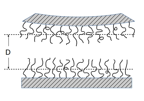
Figure 9: Sketch of polymer-coated surfaces (a), and construction of the hydrodynamic penetration length into one surface (b)

At low shearing rates with $W_{i}\leq 0.3$, the brush is almost unperturbed by the flow Doyle:1998 and thus certain hydrodynamic parameters can be linked to equilibrium brush characteristics. We study the problem of shear flow penetration into an unperturbed brush following Milner Milner:hydrodynamic who evaluated the hydrodynamic penetration depth for a parabolic monodisperse brush. Our main focus is, of course, to study the effect of brush polydispersity.

The notion of the penetration length is essential for understanding the lubrication forces that oppose the approach of a sphere of radius $R$ towards a flat surface when they are immersed in a liquid of viscosity $\eta$ (see Fig. 9). The force is described by the Reynolds formula

$$F_{\mathrm{lub}}=-6\pi R^{2}\eta\frac{\dot{D}}{D}$$ (18)

where $D$ is the closest distance between the surfaces. The Reynolds equation has been tested for solid surfaces down to surface separations of some 10 molecular diameters Klein:1996 . When the surfaces are coated with polymer brushes, the parameter $D$ refers to the separation between the points where the tangential velocity profile at the brush surface extrapolates to zero. These points coincides neither with the position of the solid substrate nor with the outer brush edge, see Fig. 9.

The penetration of a shear flow into a monodisperse brush was calculated by Milner in Ref. Milner:hydrodynamic under the assumption that the brush can be treated as a dilute porous medium, according to the seminal paper by Brinkman Brinkman:1947 , and that the inhomogeneous unperturbed brush density profile introduces a position-varying screening length $\lambda(x)$. In the absence of pressure gradients, the equation describing the tangential velocity component $v$ as a function of the distance from the outer edge of the brush, $x=H-z$, (see Fig. 9) reads:

$$\frac{d^{2}v}{dx^{2}}=\lambda^{-2}(x)v$$ (19)

Several versions were proposed for the connection between the screening length and the local monomer density $\phi$. Lai and Binder Lai:1993 assumed that the scaling expression for the correlation length in semi-dilute solutions scales as $\lambda\sim\phi^{-3/4}$, while Milner Milner:hydrodynamic used the correlation length that appears naturally in the SCF picture of a polymer brush in a good solvent, $\lambda\sim\phi^{-1}$. Suo and Whitmore Whitmore:2014 recently suggested yet another form for the relation $\lambda(\phi)$ based on a free-draining assumption for the brush chains. Here we will first adopt Milner’s approach in studying the polydispersity effects and then extend our results to include the free-draining limit.

In the simplest case of the Alexander brush with a constant density, the solution decays exponentially:

$$v(x)=v(0)e^{-x/\lambda},$$ (20)

and the resulting penetration depth $l_{p}=\lambda=1/\phi_{0}$ (where $\phi_{0}$ is the density at the grafting surface) depends only on the grafting density and not on the chain length Milner:hydrodynamic ,

$$l_{p}\sim\sigma^{-2/3}$$ (21)

For a monodisperse brush with a parabolic profile, the density near the brush edge is approximated by a linear function with the slope evaluated at $z=H_{\mathrm{mono}}$:

$$\phi(x)=2x\phi_{0}/H_{\mathrm{mono}}$$ (22)

The solution is given by Eq. (73) in Appendix C. The initial decrease of the flow velocity as it penetrates the brush is approximately linear, and the hydrodynamic penetration depth is defined as the depth where this velocity profile extrapolates to zero. The result for $l_{p}$ is presented below in Eq. (24) (top line). The predicted penetration depth is considerably larger than that obtained for the Alexander brush model (Eq. (21)), but is still much smaller than the brush thickness. The same solution is obtained for the moderately polydisperse brush with a profile close to linear in the whole range of $z$. The only modification to Eq. (73) is that the slope in the expression for $\phi(x)$ must be replaced according by $\phi(x)=x\phi_{0}/H=\frac{3}{4}x\phi_{0}/H_{\mathrm{mono}}$, which leads to the penetration depth given in the middle line of Eq. (24). In the case of a strongly polydisperse brush with $\mbox{${N_{w}}/{N_{n}}$}=2$, however, the situation changes. The brush is very tenuous near its edge, hence one can expect that the flow penetration may be more pronounced. The convex shape of the density profile suggests that a quadratic approximation to the brush profile is more appropriate than a linear one. Indeed, the exact analytical expression, Eq. (14), yields the asymptotic tail density

$$\phi(x)=\phi_{0}\left(\frac{2x}{3\pi H_{\mathrm{mono}}}\right)^{2}$$ (23)

The solution for the flow profile is given by Eq. (75) in Appendix C and yields the hydrodynamic penetration length shown in the bottom line of the equation below.

$$l_{p}=\left\{\begin{array}[]{lll}1.04\left(\frac{H_{\mathrm{mono}}}{\phi_{0}}\right)^{1/2}&\sim N_{n}^{1/2}\sigma^{-1/6}&\textrm{monodisperse }\\ 1.7\left(\frac{H_{\mathrm{mono}}}{\phi_{0}}\right)^{1/2}&\sim N_{n}^{1/2}\sigma^{-1/6}&\textrm{moderately polydisperse}\\ 4.2\left(\frac{H_{\mathrm{mono}}^{2}}{\phi_{0}}\right)^{1/3}&\sim N_{n}^{2/3}&\textrm{strongly polydisperse }\end{array}\right.$$ (24)

These scaling expressions for the penetration depth can also be derived from simple qualitative arguments. It is clear that very close to the brush edge the density is low and the flow can penetrate easily. As the density increases, the local screening length goes down and the flow is screened stronger. At some point, the local screening length becomes comparable to the distance that the flow has penetrated already, $x\sim\lambda(x)$. Beyond that point, the flow is effectively stopped. Hence the penetration depth can be estimated from a simple condition:

$$l_{p}=\lambda\left(\phi\left(l_{p}\right)\right)$$ (25)

In the case of the monodisperse or moderately polydisperse brush with $\phi(x)\sim x\phi_{0}/H_{\mathrm{mono}}$, this leads to $l_{p}\sim H_{\mathrm{mono}}/(l_{p}\phi_{0})$ and $l_{p}\sim\left(H_{\mathrm{mono}}/\phi_{0}\right)^{1/2}$, which coincides with Eq. (24) (top and middle lines) up to numerical prefactors. Likewise, in the case of the strongly polydisperse brush, the relation $\Phi(x)\sim x^{2}\phi_{0}/H_{\mathrm{mono}}$ yields $l_{p}\sim\left(H_{\mathrm{mono}}^{2}/\phi_{0}\right)^{1/3}$ in agreement with Eq. (24) (bottom).

We conclude that generally the hydrodynamic penetration depth $l_{p}$ increases with increasing polydispersity index. However, for weak to moderate polydispersities, the increase is relatively small and does not modify the scaling law $l_{p}\sim N_{n}^{1/2}\sigma^{-1/6}$. Strong polydispersity represented by an exponential chain length distribution with $\mbox{${N_{w}}/{N_{n}}$}=2$ leads to a considerably larger hydrodynamic penetration depth with a different scaling, $l_{p}\sim N_{n}^{2/3}$.

The above discussion is based on the assumption that the brush can be treated as a porous medium Milner:hydrodynamic , i.e., brush monomers are taken to act as fixed obstacles on the flow. In reality, monomers can follow the flow to some extent, and even though this does not change the density profiles significantly at low shear rates, it does affect the force balance equation that determines the flow profile in the brush. In the so-called “free-draining” limit where hydrodynamic interactions are neglected Doyle:1998 , the drag force due to flow-brush interactions becomes linear in the monomer density. A modified Brinkmann equation that conforms to the free-draining model was recently introduced in Ref. Whitmore:2014 :

$$\frac{d^{2}v}{dx^{2}}=\frac{\zeta}{\eta}\frac{\phi(x)}{1-\phi(x)}v(x)=\lambda^{-2}(x)\,v$$ (26)

Here the screening length is now related to the monomer density as $\lambda\sim\left(\frac{1-\phi}{\phi}\right)^{1/2}$. Considering only the low monomer density limit $\phi(x)\ll 1$ and omitting prefactors of order 1, we obtain

$$\frac{d^{2}v}{dx^{2}}=\phi(x)\ v.$$ (27)

Repeating the calculations for the four cases discussed above yields the following expressions for the penetration depth into free-draining brushes:

$$l_{p}=\left\{\begin{array}[]{lll}\left(\frac{H_{\mathrm{mono}}}{\phi_{0}}\right)^{1/3}&\sim N_{n}^{1/3}\sigma^{-1/9}&\textrm{monodisperse }\\ \left(\frac{H_{\mathrm{mono}}}{\phi_{0}}\right)^{1/3}&\sim N_{n}^{1/3}\sigma^{-1/9}&\textrm{moderately polydisperse}\\ \left(\frac{H_{\mathrm{mono}}^{2}}{\phi_{0}}\right)^{1/4}&\sim N_{n}^{1/2}&\textrm{strongly polydisperse }\end{array}\right.$$ (28)

All these scaling results still follow from Eq. (25), using $\lambda(\phi)=\phi^{-1/2}$. Due to the increased drag force on the solvent in the free-draining case, it is more difficult for the flow to penetrate the brush compared to the case of partially screened hydrodynamics.

We should stress again that our treatment, which was based on the assumption that the brush profile is not perturbed by the shear flow, can only be used for small shear rates. This restriction is particularly relevant in the case of strongly polydisperse brushes which are very tenuous and thus susceptible to small external forces near the outer edge. Whether the treatment presented above is valid in under prevalent experimental conditions has been a subject of some debate Klein:1996 .

The behavior of brushes in shear flow has been studied extensively by various versions of MD, dynamic MC, and DPD simulations. Some MD simulations Doyle:1998 have employed the free-draining approximation to evaluate the drag forces applied to brush chains. In contrast, Wijmans and Smit Wijmans:2002 carried out DPD simulations with explicit solvent that did not make any assumptions regarding the velocity profile in the polymer layer. Their results can be used to check the validity of theories that describe the solvent flow, such as the Brinkman equation and, in particular, the dependence of the position-dependent screening length on the local monomer density. According to these simulations for rather short brush chains with $N=20$ and several grafting densities, the data on the screening length $\lambda$ as a function of the monomer density collapse onto a master curve, giving $\lambda\sim\phi^{-0.55}$. This is in better agreement with the free-draining treatment than with the non-draining relation in the absence of swelling effects $\lambda\sim\phi^{-1}$ utilized by Milner Milner:hydrodynamic .

A direct DPD simulation of the flow penetration into a brush-coated surface and the penetration depth was recently carried out by Deng et.al. Deng:2012 . The brush was monodisperse. With the flow velocity gradients used in the simulations, the brush density profile was almost unperturbed, which corresponded to Weissenberg numbers of less than $W_{i}=1.$ The observed penetration depth was considerably smaller than the total brush height (roughly 1/10) but not small compared to atomic sizes (about 5 nm after conversion of the model parameters to ordinary units). It was shown that the penetration depth decreases with increasing grafting density, $\sigma$, although the change is not large. The scaling exponent for the $l_{p}(\sigma)$ dependence was not estimated, and the length of the brush chains was not varied.

We close this section with a brief discussion on the total shear stress experienced by the brush-coated surface. The average drag force exerted by the flowing solvent on the brush-coated surface depends on the velocity profile, which, in turn, is determined by details of the brush-flow interaction. Under stationary conditions, the force balance requirement results in a simple identity that could provide a useful test to check the consistency of the numerical work. Imagine a pair of opposing surfaces in Couette geometry, one of which is brush-coated and the other is bare. The shear stress acting on the bare surface is completely determined by the velocity gradient at the boundary $\eta\dot{\gamma}$. This gradient is the same across the gap where only pure solvent is flowing, down to the outer brush edge and can be accurately measured in simulations. The total drag per unit area of the brush-coated surface must always be given by the same expression, irrespective of the brush parameters or the detailed way of treating hydrodynamics. Thus the value of the stationary velocity gradient outside the brush encodes all the relevant information on the brush-flow interaction.

VII Summary: Main features of polydisperse brushes

The main focus of the present paper was to systematically compare the equilibrium and hydrodynamic properties of monodisperse and polydisperse brushes. We first recapitulate some very general results that have first been obtained by Milner, Witten, and Cates Milner_Polydisp for arbitrary molecular mass distributions, but have remain underappreciated in the current literature in our opinion:

1.) Under good solvent conditions and in the strong crowding limit, the monomer density at the grafting surface, $\phi_{0}$, is determined only by $\sigma$ and the excluded volume parameter, $v$:

$$\phi_{0}=\frac{3}{2}\left(\frac{\pi\sigma v}{2}\right)^{2/3}$$

and depends neither on the average chain length, nor on the shape of the chain length distribution. In simulations, one observes some decrease in the brush density near the surface for larger polydispersities which is a finite-$N$ effect that would disappear in the asymptotic limit.

2.) Under the same conditions, the brush height always scales as:

$$H\sim N_{n}\sigma^{1/3}$$

irrespective of the particular shape of the chain length distribution and of the polydispersity index. The prefactor, however, is a function of the chain length distribution and typically increases with the polydispersity parameter.

Turning to our own results, in the following, we summarize the changes in the brush properties produced by polydispersity effect. In the present paper we have mostly focussed on the Schultz-Zimm family of molecular mass distributions, and hence a polydisperse brush is uniquely characterized by 3 parameters: the number-averaged molecular mass (or polymerization index), $N_{n}$, the grafting density, $\sigma$, and the polydispersity index ${N_{w}}/{N_{n}}$ .

3.) At fixed $N_{n}$ and $\sigma$, the brush height increases with the polydispersity parameter, which can be approximately described by a very simple expression as demonstrated in Fig. 2.

4.) With increasing polydispersity, the shape of the brush density profile systematically changes from the concave down parabolic shape to a convex shape. At moderate polydispersity, $\mbox{${N_{w}}/{N_{n}}$}\backsimeq 1.15$ the profile is close to linear with a constant slope (see Fig. 1).

5.) A monodisperse brush is characterized by anomalous chain end fluctuations $\mathrm{var}Z_{N}\sim H^{2}$ due to the fact that the end monomer of each chain explores all the space within the brush thickness. In a polydisperse brush, the end of each chain fluctuates around its own mean position. With increasing polydispersity, the anomalous fluctuations are suppressed as illustrated by Fig. 8, so that eventually the fluctuations of a typical chain recover the ideal behavior $\mathrm{var}Z_{N_{n}}\sim N_{n}$ .

At least two effects are expected as consequences of this change. The first is related to chain relaxation dynamics. A monodisperse unentangled brush exhibits very large relaxation times $\tau\sim N_{n}^{3}$; however, we expect Rouse relaxation times $\tau\sim N_{n}^{2}$ to be restored even in moderately polydisperse brushes. For longer chain lengths $N_{n}$, entanglement effects become important. A recent study on dense monodisperse polymer brushes showed that the relaxation time scales exponentially with the chain length $N_{n}$ with the prefactor $N_{n}^{3}$, i.e., $\tau\propto N_{n}^{3}\exp(N_{n}/N_{e})$ where $N_{e}$ is the entanglement degree entanglement_brush . We would expect that when the entanglement is involved, the relaxation time might be reduced to $\tau\sim N_{n}^{2}\exp(N_{n}/N_{e})$ even in moderately polydisperse brushes. The second consequence relates to the effect reported in Refs. Merlitz:2008 ; Romeis:2012 as “surface instability” of a monodisperse brush: The modification of the end-group of some brush chains so that it becomes sensitive to small variations in the solvent quality results in a possibility of an abrupt transition for the modified chains either “hiding” inside the brush or exposing the end-group at the outer brush edge. The transition is clearly linked to the anomalously high susceptibility of chain ends in a monodisperse brush. As the latter is strongly suppressed by polydispersity, we expect the surface instability to be affected as well.

6.) Hydrodynamic flow near a brush-coated surface penetrates into the brush. The penetration depth, $l_{p}$, increases with the polydispersity since the brush becomes more tenuous at the edge. For moderate polydispersities the effect is not very large, but for $\mbox{${N_{w}}/{N_{n}}$}=2$ we predict a stronger scaling $l_{p}\sim N_{n}^{2/3}$ as opposed to $l_{p}\sim N_{n}^{1/2}\sigma^{-1/6}$ in the monodisperse case.

We hope that the relatively simple picture of polydisperse brushes, their internal structure and related properties, which we have presented here, may be useful for researchers developing new methods of brush synthesis and applications of brush-coated surfaces.

ACKNOWLEDGMENTS

Financial support by the Deutsche Forschungsgemeinschaft (Grants No. SCHM 985/13-2) is gratefully acknowledged. S. Qi acknowledges support from the German Science Foundation (DFG) within project C1 in SFB TRR 146. Simulations have been carried out on the computer cluster Mogon at JGU Mainz.

Appendix A Numerical SCF theory

In the SCF approach SCF_R1 ; SCF_book , the configurational partition function is converted to path integrals over the fluctuating fields by invoking functional delta constraints. One obtains $\mathcal{Z}=\int\mathcal{D}\omega\mathcal{D}\rho_{t}e^{-\beta\mathcal{F}}$ with the free energy functional expressed as

$$\beta\mathcal{F} = \frac{v}{2}\int d\mathbf{r}\phi^{2}-\int d\mathbf{r}\omega\phi-\sum_{\alpha=1}^{n_{b}}\ln Q_{\alpha}[\omega]$$ (29)

where $\phi$ is the total fluctuating density, $\omega$ is the corresponding conjugate auxiliary potential, and $Q_{\alpha}$ is the single chain partition functions for the $\alpha$-th chain. For a system with macroscopic volume $V$, we assume that the sum over all brush chains can be replaced by a continuous integral weighted by a proper continuous chain length distributions, which means

$$\sum_{\alpha=1}^{n_{b}}\ln Q_{\alpha}[\omega]\simeq n_{b}\int_{0}^{\infty}dNP(N)\ln Q(N,\omega)$$ (30)

where $Q$ is the partition function of a brush chain with chain length $N$, and $P(N)$ is defined as the quenched chain length distribution function normalized to unity $\int_{0}^{\infty}dNP(N)=1$. Extremizing the free energy functional with respect to the fluctuating fields, i.e., the density $\phi$ and the potential $\omega$, we obtain a set of closed SCF equations

$$\omega = v\phi$$ (31)

$$\phi = n_{b}\int_{0}^{\infty}dNP(N)\frac{1}{Q(N)}\int_{0}^{N}dsq(\mathbf{r},s)q^{\dagger}(\mathbf{r},N-s)$$

where the single chain partition function can be calculated from the propagators, i.e., $Q_{N}=\int d\mathbf{r}q^{\dagger}(\mathbf{r},N)$. The propagators $q^{\dagger}$ and $q$ satisfy the same modified diffusion equation

$$\frac{\partial q(\mathbf{r},s)}{\partial s}=\frac{b^{2}}{6}\nabla^{2}q(\mathbf{r},s)-\omega(\mathbf{r})q(\mathbf{r},s)$$ (32)

but with different initial conditions. We use the initial condition $q(\mathbf{r},0)=1$, and $q_{\dagger}(\mathbf{r},0)=\delta(z)$, i.e., one end of each chain is free, while the other end is grafted at $z=0$ with mobile grafting point. Since the grafting substrate is impenetrable for all chains, we implement Dirichlet boundary condition there.

Inserting the SZ distribution function $P(N)$ into the density $\phi$, we obtain

$$\phi = \frac{n}{\Gamma(k)}\int_{0}^{\infty}dxx^{k-1}e^{-x}$$ (33)

$$\times \frac{1}{Q[xN_{n}/k]}\int_{0}^{xN_{n}/k}dsq(\mathbf{r},s)q^{\dagger}(\mathbf{r},xN_{n}/k-s)$$

where $x=kN/N_{n}$. In practice, the above infinite integration is approximated by the Gauss-Laguerre quadrature numerical_recipes , which has the form of

$$\int_{0}^{\infty}dxx^{k-1}e^{-x}f(x)=\sum_{j=1}^{n_{G}}w_{j}f(x_{j})$$ (34)

where the abscissae ($x_{j}$) and weights ($w_{j}$) can be evaluated numerically. This quadrature normal converges very rapidly. For example, for a polymer blend, $n_{G}\lesssim 10$ is enough to generate converged interfaces. For the present brush system, we found that several ten points are necessary to obtain smooth and accurate brush density profiles. With a smaller number of sampled chain lengths, the obtained brush densities are not so smooth. In the present paper, we adopt $n_{G}=60$. The modified diffusion equation is solved in real space using the Crank-Nicolson scheme, which is a finite difference method. The SCF equations are solved iteratively by updating the potential $\omega$ with a simple mixing scheme. In the main text we consider only the one dimensional system.

Appendix B Structure of polydisperse brushes: theory

B.1 Analytical SCF theory in the strong stretching approximation

An important quantity that needs to be specified in order to characterize the structure properties of a polydisperse polymer brush is the self-consistent potential $\omega(z)$. At the mean field level, in good solvent, this potential is proportional to the monomer density with the proportionality constant being the excluded volume parameter.

We begin with briefly describing the mean-field approach we use to evaluate the potential. It is based on the MWC theory Milner_Polydisp . Our goal is to derive an expression for the potential as a function of the distance from the substrate, i.e., the spatial coordinate $z$. We assume that the potential is a monotonically decreasing function of $z$ with its maximum a $z=0$, where the monomer density is high, and that it vanishes at the brush edge $z=H$. The potential can then be written as $\omega=A-U$, where $U$ is a monotonically increasing function with $U=0$ at $z=0$ and $U=A$ at $z=H$. For $0<z<H$ there hence exists a unique relation between $z$ and $U$.

Apart from the mean-field approximation, we also adopt the strong stretching approximation, i.e., we assume that chains never loop back, and take the asymptotically long chain limit whereby fluctuations can be neglected. As demonstrated in the MWC theory Milner_Polydisp , the density and the potential are connected through the free end distribution $\Phi_{e}(z)$ via

$$\phi(z)=\Big{(}\frac{3}{2}\Big{)}^{1/2}\int_{U(z)}^{A}dU^{\prime}\frac{\epsilon(U^{\prime})}{\sqrt{U^{\prime}-U(z)}}$$ (35)

in this limit, where we have defined $\epsilon(U)=\Phi_{e}(z)\>dz/dU$. Since we have $\phi(z)=A-U(z)$ for a brush at the mean field level (note again that we set $v=1$), this equation implies the relation $\epsilon(U)=\sqrt{\frac{8}{3\pi^{2}}}(A-U)^{1/2}$. From $\epsilon(U)$, we can define a cumulative grafting density $\sigma_{c}(z)$, corresponding to the number of polymer chains per unit area with chain end position at distance smaller than $z(U)$ from the substrate, i.e., $\sigma_{c}[U]=\int_{0}^{U}dU^{\prime}\epsilon(U^{\prime})$. Inserting the expression for $\epsilon$, we can express the cumulative grafting density as a function of $U$,

$$\sigma_{c}(U)=\sqrt{\frac{8}{3\pi^{2}}}\frac{2}{3}A^{3/2}\Big{[}1-\Big{(}1-\frac{U}{A}\Big{)}^{3/2}\Big{]}.$$ (36)

As the total grafting density for all chains is fixed to be $\sigma$, which requires $\sigma_{c}(A)=\sigma$, we have $\sigma=\sqrt{\frac{8}{3}}\frac{2}{3\pi}A^{3/2}$, or in other words,

$$A=\frac{3}{2}\big{(}\frac{\pi\sigma}{2}\big{)}^{2/3}.$$ (37)

This implies that the monomer density at the grafting surface $z=0$ is only determined by the total grafting density, independent of the polydispersity.

In a polydisperse brush, according to the strong segregation approximation, chains with different lengths are completely segregated, and there is a unique relation between the chain length $N$, the position of the end monomer $z$, and the corresponding value of $U(z)$. Hence we can associate $\sigma_{c}(U)$ with the cumulative grafting density $\sigma_{c}(N)$ of chains with length shorter than $N$, and from Eq. (36), we can express $U$ as a function of $\sigma_{c}(N)$, i.e.,

$$U(N)=A\Big{[}1-\Big{(}1-\frac{\sigma_{c}(N)}{\sigma}\Big{)}^{2/3}\Big{]}$$ (38)

On the other hand, the inverse function, $N(U)$, obeys

$$N(U)=\int_{0}^{U}dU^{\prime}\frac{dN}{dU^{\prime}}=\sqrt{\frac{3}{2}}\int_{0}^{U}dU^{\prime}\frac{dz}{dU^{\prime}}\frac{1}{\sqrt{U-U^{\prime}}}$$ (39)

in the strong stretching theory Milner_Polydisp , and one can easily see that this equation is fulfilled if

$$\frac{dz}{dU}=\sqrt{\frac{2}{3\pi^{2}}}\int_{0}^{U}dU^{\prime}\frac{dN}{dU^{\prime}}\frac{1}{\sqrt{U-U^{\prime}}}.$$ (40)

From these equations we can obtain $U(z)$ is $N(U)$ is explicitly known.

Finally, Eq. (40) may be integrated to find a general expression for the equilibrium height:

$$H=\frac{2}{\pi}\sqrt{\frac{2}{3}}\int_{0}^{N_{\mathrm{max}}}dn\left(A-U(n)\right)^{1/2}$$ (41)

Since every chain length distribution with a finite first moment can be written in the form $P(N)=N_{n}^{-1}\psi\left(\frac{N}{N_{n}}\right)$, it follows from Eq. (38) that $U(n)/A$ is a function of the reduced variable $\frac{n}{N_{n}}$ only, the values of the function being in the range [0,1]. Rescaling the integration variable, $n=N_{n}t$ we arrive at

$$H=N_{n}\frac{2}{\pi}\sqrt{\frac{2A}{3}}\int_{0}^{\frac{N_{max}}{N_{n}}}dt\left(1-\frac{U(t)}{A}\right)^{1/2}$$ (42)

Substituting $A$ from Eq. (37) we obtain

$$H=\left(\frac{2}{\pi}\right)^{2/3}N_{n}\sigma^{1/3}\int_{0}^{\frac{N_{\mathrm{max}}}{N_{n}}}dt\left(1-\frac{U(t)}{A}\right)^{1/2}$$ (43)

The integral is a pure number that is determined solely by the shape of the chain length distribution but does not depend on $\sigma$ or $N_{n}$. Thus the scaling relation

$$H\sim N_{n}\sigma^{1/3}$$ (44)

is generally valid for any non-pathological chain length distribution. For a monodisperse brush the integral is reduced to $\int_{0}^{1}dt\left(1-\theta(t-1)\right)^{1/2}=1.$ For any other chain length distribution it will have the meaning of $\frac{H}{H_{\mathrm{mono}}}$. As another simple illustration, we note that for an exponential distribution density, Eq. (68) leads to the explicit form $\int_{0}^{\infty}dt\exp\left(-\frac{t}{3}\right)=3$.

B.2 Monodisperse brush with a vanishing fraction of minority chains of different length

The monodisperse brush corresponds to the very special limit where $N(U)$ in Eq. (39) is a constant, $N(U)\equiv N_{n}$. Even though the assumption of chain length segregation obviously breaks down in this limit, and the function $N(U)$ cannot be inverted, all equations of the previous section except Eq. (38) still hold (with $dN/dU=N_{n}\>\lim_{\epsilon\to 0^{+}}\delta(U-\epsilon)$) and Eq. (40) immediately gives $U(z)=-\frac{3\pi^{2}}{8N_{n}^{2}}z^{2}$.

Here we summarize the main structural properties of monodisperse brushes. The density profile is given by:

$$\phi(z)=\phi(0)\left(1-\frac{z^{2}}{H_{\mathrm{mono}}^{2}}\right)$$ (45)

where $\phi(0)=\frac{3}{2}\left(\frac{\pi\sigma}{2}\right)^{2/3}$. The brush height

$$H_{\mathrm{mono}}=\left(\frac{4v\sigma}{\pi^{2}}\right)^{1/3}N_{n}$$ (46)

scales linearly with the chain length $N_{n}$. The brush density generates the chemical potential profile:

$$\omega(z)=\frac{3\pi^{2}}{8N_{n}^{2}}(H_{\mathrm{mono}}^{2}-z^{2})$$ (47)

Next we introduce a vanishing fraction of minority chains of different length, $N$, into the otherwise monodisperse brush. The Green’s function of a minority chain is given by the known solution of the Edwards’ equation

$$\frac{\partial G(z,s)}{\partial s}=\frac{1}{6}\frac{\partial^{2}G(z,s)}{\partial^{2}z}-\omega(z)G(z,s)$$ (48)

in the presence of a parabolic potential Eq. (47) and an impenetrable inert grafting surface Skvortsov:1997 :

$$G(z,N)=B\>z\exp\left[-\frac{3\pi}{4N_{n}}\cot\left(\frac{\pi N}{2N_{n}}\right)z^{2}\right]$$ (49)

Here $B$ is a normalization factor. If minority chains are longer or equal to the mean length of the majority chain, $N\geq N_{n}$, the Green’s function Eq. (49) shows an unbounded monotonic increase with $z$ since the solution refers to a potential extending to infinity and an ideal Gaussian chain with unlimited extensibility. Even chains slightly shorter than $N_{n}$ are predicted to extend beyond the brush edge at $z=H_{\mathrm{mono}}$. However, the brush edge modifies the potential at $z>H$ dramatically which roughly amounts to a truncation of the Green’s function Eq. (49) at $z=H_{\mathrm{mono}}$ for chains with $N\leq N_{n}$. Comparison with numerical SCF calculations shows that for longer chains, $N\geq N_{n}$, the truncated Green’s function describes well the position of the $N_{n}$-th monomer, while the last $N-N_{n}$ monomers have a mushroom-like configuration with the average end-to-end distance of $[\pi(N-N_{n})/6]^{1/2}$. Obtaining the full expression for the average distance of the free end $Z_{e}(N)$ is rather cumbersome, but most of the curve can be described by two simple limits:

$$Z_{\mathrm{e}}(N)=\left\{\begin{array}[]{ll}\left[\frac{N_{n}}{3}\tan\left(\frac{\pi N}{2N_{n}}\right)\right]^{1/2},&N<N_{n}\\ H_{\mathrm{mono}}-\frac{4N_{n}^{2}}{3\pi^{2}H(N-N_{n})}+\left[\frac{\pi(N-N_{n})}{6}\right]^{1/2},&N>N_{n}\end{array}\right.$$ (50)

where the difference $|N-N_{n}|$ must be at least a few units for the approximation to be meaningful. Similarly, the variance of the end-monomer position var$Z_{N}$ is evaluated using the truncated Green’s function for $N\leq N_{n}$, while for $N>N_{n}$ an extra term $\frac{(4-\pi)}{6}(N-N_{n})$ accounting for the terminal subchain with a mushroom configuration is added. For the fluctuations of the end-monomer positions we have two simple limits:

$$\mathrm{var}Z_{N}=\left\{\begin{array}[]{ll}\frac{(4-\pi)}{3\pi}N_{n}\tan\Big{(}\frac{\pi N}{2N_{n}}\Big{)},&N<N_{n}\\ \frac{16N_{n}^{4}}{9\pi^{4}H_{\mathrm{mono}}^{2}(N-N_{n})^{2}}+\frac{(4-\pi)}{6}(N-N_{n}),&N>N_{n}\end{array}\right.$$ (51)

B.3 Weakly polydisperse brush

A monodisperse brush is characterized by the relation $\frac{U(N)}{A}=\Theta(N-N_{n})$. To introduce an analytically tractable model of weakly polydisperse brushes we replace the $\Theta$-function by a function which is reminiscent of the well-known low-temperature limit of the Fermi-Dirac hole occupancy:

$$\frac{U(N)}{A}=1-\frac{1}{\exp\left(\frac{1}{\Delta}\left(\frac{N}{N_{n}}-1\right)\right)+1}$$ (52)

where $\Delta$ is a small parameter analogous to the reduced temperature $\frac{T}{T_{F}}$ in the Fermi gas: It gives the relative width of the “smoothing”. In the language of the chain length distribution density, $P\left(\frac{N}{N_{n}}\right)$, $\Delta$ also defines its width. For a narrow distribution of relative width $\Delta,$ $N_{w}\sim N_{n}\left(1+\Delta^{2}\right)$, leading to

$$\Delta\sim\left(\mbox{${N_{w}}/{N_{n}}$}-1\right)^{1/2}$$ (53)

Solving Eq. (52) for $N(U)$ and substituting into Eq. (40) gives:

$$\frac{dz}{dU} = \sqrt{\frac{2}{3A}}\frac{N_{n}}{\pi}\frac{1}{\sqrt{U}}\Bigg{[}1+\Delta\Big{(}\log\frac{4U}{A}$$ (54)

$$+\;2\sqrt{\frac{U}{A-U}}\arctan\big{(}\frac{U}{A-U}\big{)}\Big{)}\Bigg{]}$$

(note that in this case, the lower bound in the integral (40) and $\int dU^{\prime}\frac{dz}{dU^{\prime}}$ cannot be set to zero, but must be chosen $U(0)\approx\exp(-\frac{1}{\Delta})\neq 0$).

Our main focus is to estimate the second derivative $\frac{d^{2}U}{dz^{2}}$ which is expressed as

$$\frac{d^{2}U}{dz^{2}}=-\left(\frac{dz}{dU}\right)^{-3}\frac{d}{dU}\left(\frac{dz}{dU}\right)$$ (55)

up to terms linear in the small parameter

$$\frac{d^{2}U}{dz^{2}}=3\left(\frac{\pi}{2N_{n}}\right)^{2}\left(1-\Delta\psi\left(\frac{U}{A}\right)\right),$$ (56)

where $\psi\left(\frac{U}{A}\right)$ is obtained from Eq. (54) and positive for $U/A>0.07$. Hence the curvature of the mean-force potential is indeed reduced, the relative reduction being linear in $\Delta$. Evaluating the function $\psi$ close to the middle point of the brush, $U/A=1/2$ we obtain an approximation for the typical curvature of the potential:

$$\frac{d^{2}U}{dz^{2}}=3\left(\frac{\pi}{2N_{n}}\right)^{2}\left(1-c\Delta\right)$$ (57)

with $c\approx 6$. Now the fluctuations of a chain with $N=N_{n}$ can be obtained from the Green’s function Eq. (49) modified to account for the reduced coefficient in the parabolic potential:

$$G(z,N_{n})=B\>z\exp\left[-\frac{3\pi}{4N_{n}}\cot\left(\frac{\pi}{2}\left(1-\frac{c}{2}\Delta\right)\right)z^{2}\right]$$ (58)

In the limit of $\Delta\ll 1$ the fluctuations scale as

$$\mathrm{var}Z_{N_{n}}\sim N_{n}\Delta^{-1}\sim N_{n}\left(\mbox{${N_{w}}/{N_{n}}$}-1\right)^{-1/2},$$ (59)

as long as they don’t exceed those in a purely monodisperse brush.

B.4 Moderately polydisperse brush with exactly linear density profile

The density profile of a brush formed by chains with SZ distribution at $\mbox{${N_{w}}/{N_{n}}$}=1.143$ ($k=7$), is reasonably close to a linear shape. From a theoretical point of view this presents a considerable advantage since the Green’s function of an ideal chain placed in a linear potential is known Mansfield . Equally fortunately, one can also find a closed-form analytical description of a polydisperse brush with exactly linear profile within the SCF strong-stretching approximation. We write the linear density profile as

$$\phi_{\mathrm{lin}}(z)=\phi_{0}-fz$$ (60)

where we have discussed that $\phi_{0}\equiv A$ has nothing to do with the polydispersity. From the density profile, the height of the brush can be defined as $H=\phi_{0}/f$. The slope $f$ can be specified according to the fact that the total number of monomers in the system are fixed to be $\sigma N_{n}$, i.e., one can get $f=\phi_{0}^{2}/(2\sigma N_{n})$. According to our previous notation, we have $U=fz$, and thus $dz/dU=1/f$. According to Eq. (39), we obtain $N(U)=\sqrt{6U}/f$, from which we have $U=f^{2}N^{2}/6$. Subsequently, we can evaluate the cumulative grafting density according to Eq. (36)

$$\frac{\sigma_{c}(N)}{\sigma}=\left[1-\left(1-\frac{f^{2}N^{2}}{6A}\right)^{3/2}\right]$$ (61)

The derivative of $\sigma_{c}(N)/\sigma$ with respect to $N$ gives the chain length distribution function

$$P_{\mathrm{lin}}(N)=\frac{3N}{N_{\mathrm{max}}^{2}}\left[1-\frac{N^{2}}{N_{\mathrm{max}}^{2}}\right]^{1/2}$$ (62)

where the cut-off chain length $N_{\mathrm{max}}$ is defined as $N_{\mathrm{max}}=\sqrt{6A}/f=\frac{16}{3\pi}N_{n}$. It can be checked that this chain length distribution is normalized to 1, and the number-averaged chain length is equal to $N_{n}$ as expected. The polydispersity index can be directly calculated as $\mbox{${N_{w}}/{N_{n}}$}=1.153$, which is quite close to that of the SZ distribution with $k=7$ although the actual shape differs as demonstrated in Fig. 6(a) and Fig. 6(d) (insets). In terms of $H_{\mathrm{mono}}$ with the same parameter $\sigma$ and $N_{n}$ given by Eq. (46), the brush thickness of the moderate polydisperse brush can be expressed as $H=\frac{4}{3}H_{\mathrm{mono}}$. It is a puzzling coincidence that the form of the chain length distribution given by Eq. (62) is the same as the end monomer density distribution in a monodisperse brush.

A linear density profile generates a uniform constant stretching force acting on each monomer, very similar to a gravitational field. The Green’s function of a chain placed in a uniform force field of strength $f$ is a solution of the Edwards’ equation (Eq. (48)) with $\omega(z)=-fz$, which was obtained in Ref. Mansfield :

$$G(z,N)=\left(\frac{2\pi N}{3}\right)^{-1/2}\exp\left[\frac{f^{2}N^{3}}{18}-\frac{3}{2N}\left(z-\frac{f\,N^{2}}{6}\right)^{2}\right]$$ (63)

A closely related solution in the context of quantum mechanics (propagator for a non-relativistic particle in an accelerator) has also been known Feynman . The polymer Green’s function was used to describe properties of a chain in a viscous flow or of a charged chain in a uniform electric field. It is quite striking that a polydisperse brush turns out to be another possible source of a linear potential. The force $f$ is to be identified with the slope of the linear density profile:

$$f=\frac{9\pi}{16N_{n}}\left(\frac{\pi\sigma}{2}\right)^{1/3}$$ (64)

For a semi-quantitative comparison of the theory with the MC data, the effect of the impenetrable grafting surface and the cut-off of the field for $z>H$, i.e., beyond the brush edge, must be taken into account. This is done in manner similar to the monodisperse case:

$$G(z,N)=B^{\prime}\>z\ \exp\left[-\frac{3}{2N}\left(z-\frac{fN^{2}}{6}\right)^{2}\right],\qquad z\leq H,$$ (65)

where $B^{\prime}$ is a normalization constant

Like in the monodisperse case, the Green’s function (Eq. (63)) is used to evaluate $Z_{e}(N)$ and var$Z_{N}$ for chains with $N\leq N_{\mathrm{max}}$. For longer chains, these values are interpreted as referring to the $N_{\mathrm{max}}$-th monomer, and the contributions due to the mushroom-like tail of length $(N-N_{\mathrm{max}})$ are added in the same way as in Sec. B.2, except that $N_{n}$ is replaced by $N_{\mathrm{max}}$ here.

B.5 Strongly polydisperse brush

The SZ distribution with $\mbox{${N_{w}}/{N_{n}}$}=2$ ($k=1$ ) has a simple exponential shape:

$$P(N)=\frac{1}{N_{n}}\exp\left(-\frac{N}{N_{n}}\right)\$$ (66)

This allows a closed-form analytical solution within the framework of the theory developed by Milner, Witten, and Cates (MWC) MWC . The cumulative grafting density (distribution) $\sigma_{c}(N)$ which plays a central role in the theory can be calculated directly as

$$\frac{\sigma_{c}(N)}{\sigma}=\int_{0}^{N}dN^{\prime}P(N^{\prime})=\left[1-\exp\left(-\frac{N}{N_{n}}\right)\right]$$ (67)

The chain length as a function of $U$ can be obtained according to Eq. (38)

$$U(N)=A\left[1-\exp\left(-\frac{2N}{3N_{n}}\right)\right],$$ (68)

from which we have the derivative

$$\frac{dN}{dU}=\frac{3}{2}\frac{N_{n}}{\left(A-U\right)}.$$ (69)

Inserting this above equation into Eq. (40) and performing the integration, we get

$$\frac{dz}{dU}=\sqrt{\frac{6N_{n}^{2}}{\pi^{2}}}(A-U)^{-1/2}\arcsin\sqrt{\frac{U}{A}}.$$ (70)

Integrating this equation, we get

$$z(U)=\frac{6N_{n}}{\pi}\Big{(}\frac{2A}{3}\Big{)}^{1/2}\left[\sqrt{\frac{U}{A}}-\sqrt{1-\frac{U}{A}}\arcsin\sqrt{\frac{U}{A}}\right].$$ (71)

We recall that according to the MWC theory, the density at the grafting surface is defined solely by the total grafting density and the number-averaged chain length, irrespective of the polydispersity, $\phi(0)=A$. Recognizing that $U/A=1-\phi/\phi(0)$, $H_{\mathrm{mono}}=\frac{2}{\pi}\sqrt{2A/3}N_{n}$, one can express the density profile as:

$$\phi_{\mathrm{exp}}(z)=\phi(0)\cdot\Psi\left(\frac{z}{3H_{\mathrm{mono}}}\right),$$ (72)

where $y=\Psi(x)$ is the inverse of the function $x=\sqrt{1-y}-\sqrt{y}\arcsin(\sqrt{1-y})$. The density profile terminates at the distance $z=3H_{\mathrm{mono}}$. The end monomer position as a function of the chain length is found by substituting $U(N)$ from Eq. (68) into Eq. (71) and identifying $z(U(N))$ with $Z_{e}(N)$, which serves approximately as the average position of the free end monomer.

Appendix C Polydisperse Brush in Hydrodynamic Shear Flow

The solution of the Brinkman equation (Eq. (19)) with $\lambda=\phi^{-1}$ and the density profile given by Eq. (22) for monodisperse brush was obtained by Milner Milner:hydrodynamic and has the form

$$v(x)=\frac{v(0)}{\Gamma(1/4)}\left(2x\sqrt{\frac{2\phi_{0}}{H_{\mathrm{mono}}}}\right)^{1/2}K_{1/4}\left(x^{2}\frac{\phi_{0}}{H_{\mathrm{mono}}}\right)$$ (73)

where $K$ is the modified Bessel function, and $\Gamma$ is the Euler gamma function. The numerical prefactor in the expression for the penetration depth is obtained from the initial slope of the function.

For the strongly polydisperse brush with $\mbox{${N_{w}}/{N_{n}}$}=2$, i.e., the density profile given by Eq. (23), we introduce the dimensionless variable $y=x\phi_{0}^{1/3}\left(\frac{2}{3\pi H_{\mathrm{mono}}}\right)^{2/3}$. The Brinkman equation (19) then reduces to:

$$\frac{d^{2}v}{dy^{2}}=y^{4}v,$$ (74)

which has an exact solution of the form

$$v(y)=v(0)\,\frac{\Gamma(5/6)}{\pi 6^{1/6}}\,K_{1/6}\left(\frac{y^{3}}{3}\right)$$ (75)

References

Alexander, S. J. Adsorption of chain molecules with a polar head a scaling description. J. Phys. France 1977, 38, 983-987.

Bixler, G. D.; Bhushan B. Biofouling: lessons from nature. Philos. Trans. R. Soc. A 2012, 370, 2381-2417.

Klein, J.; Perahia, D.; Warburg, S. Forces between polymer-bearing surfaces undergoing shear. Nature 1991, 352, 143-145.

Singh, M. K.; Ilg, P.; Espinosa-Marzal, R. M.; Kröger, M.; Spencer, N. D. Polymer brushes under shear: molecular dynamics simulations compared to experiments. Langmuir 2015, 31, 4798-4805.

Zdyrko, B.; Klep, V.; Li, X.; Kang, Q.; Minko, S.; Wen, X.; Luzinov, I. Polymer brushes as active nanolayers for tunable bacteria adhesion. Materials Science and Engineering: C 2009, 29, 680-684.

Ayres, N. Polymer brushes: applications in biomaterials and nanotechnology. Polym. Chem. 2010, 1, 769-777.

Marek, U. U. Handbook of Stimuli-Responsive Materials; Viley-VCH Verlag GmbH & Co. KGaA: Weinheim, Germany, 2001.

Cohen Stuart, M. A.; Huck, W. T. S.; Genzer, J.; Müller, M.; Ober, C.; Stamm, M.; Sukhorukov, G. B.; Szleifer, I.; Tsukruk, V. V.; Urban, M.; Winnik, F.; Zauscher, S.; Luzinov, I.; Minko, S. Emerging applications of stimuli-responsive polymer materials. Nat. Mater. 2010, 9, 101-113.

Milner, S.; Witten, T.; Cates, M. Theory of grafted polymer brush. Macromolecules 1988, 21, 2610-2619.

Zhulina, E. B.; Borisov, O. V.; Priamitsyn, V. A. Theory of steric stabilization of colloid dispersions by grafted polymers. Coll. Interface Sci. 1990, 137, 495-511.

Skvortsov, A. M.; Pavlushkov, I. V.; Gorbunov, A. A.; Zhulina, E. B.; Borisov, O. V.; Priamitsyn, V. A. Structure of densely grafted polymeric monolayers. Vysokomol. Soedin. A 1988, 30, 1598.

Advincular, R. C.; Brittain, W. J.; Caster, K. C.; Ruhe, J. Polymer Brush; Viley-VCH, Weinheim, Germany, 2011.

Binder, K.; Kreer, T.; Milchev, A. Polymer brushes under flow and in other out-of-equilibrium conditions. Soft Matter 2011, 7, 7159-7172.

Halperin, A.; Tirrell, M.; Lodge, T. P. Tethered chains in polymer microstructures. Adv. Polym. Sci. 1992, 100, 31-71.

Romeis, D.; Merlitz, H.; Sommer, J.-U. A new numerical approach to dense polymer brushes and surface instabilities. J. Chem. Phys. 2012, 136, 044903.

Naji, A.; Seidel. C.; Netz, R. R. Theoretical approaches to neutral and charged polymer brushes. Adv. Polym. Sci. 2006, 198, 149-183.

Netz, R. R.; Schick, M. Polymer brushes: from self-consistent field theory to classical theory. Macromolecules 1998, 31, 5105-5122.

Laradji, A. M.; McNitt, C. D.; Yadavalli, N. S.; Popik, V. V.; Minko, S. Roubust, solvent-free, catalyst-free click chemistry for the generation of highly stable densely grafted poly(ethylene glycol) polymer brushes by the grafting to method and theory properties. Macromolecules 2016, 49, 7625.

Turgman, C. S.; Srogl, J.; Kiserow, D.; Genzer, J. On-demand degrafting and the study of molecular weight and grafting density of Poly(methyl methacrylate) brushes on flat silica substrates. Langmuir 2015, 31, 2372-2381.

Pandav, G.; Ganesan, V.; Fluctuation effects on the order-disorder transition in polydisperse copolymer melts. J. Chem. Phys. 2013, 139, 214905.

Balko, S. M.; Kreer, T.; Costanzo, P. J.; Patten, T. E.; Johner, A.; Kuhl, T. L.; Marques, C. M. Polymer brushes under high load. PloS ONE 2013, 8(3): e58392.

Murata, H.; Koepsel, R. R.; Matyjaszewski, K.; Russell, A. J. Permanent, non-leaching antibacterial surfaces-2: How high density cationic surfaces kill bacterial cells. Biomaterials 2007, 28, 4870-4879.

Krishnamoorthy, M.; Hakobyan, S.; Ramstedt, M.; Gautrot, J. E. Surface-initiated polymer brushes in the biomedical field: applications in membrane science, biosensing, cell culture, regenerative medicine and antibacterial coatings. Chem. Rev. 2014, 114, 10976-11026.

Milner, S.; Witten, T.; Cates, M. Effects of polydispersity in the end-grafted polymer brush. Macromolecules 1989, 22, 853-861.

de Vos, W. M.; Leermakers, F. A. M. Modeling the structure of a polydisperse polymer brush. Polymer 2009, 50, 305-316.

de Vos, W. M.; Leermakers, W. M.; de Keizer, A.; Cohen Stuart, M. A. Interaction of particles with a polydisperse brush: A self-consistent-field analysis. Macromolecules 2009, 42, 5881-5891.

Helfand, E. Theory of inhomogeneous polymers: Fundamentals of the Gaussian random‐walk model. J. Chem. Phys. 1975, 62, 999-1005

Laradji M.; Guo H.; Zuckermann M. J. Off-lattice Monte Carlo simulation of polymer brushes in good solvents. Phys. Rev. E 1994, 49, 3199-3206.

Besold, G.; Guo, H.; Zuckermann, M. J. Off-lattice Monte Carlo simulation of the discrete Edwards model. J. Polym. Sci. Part B: Polym. Phys. 2000, 38, 1053-1068.

Qi, S.; Behringer, H.; Schmid, F. Using field theory to construct hybrid particle-continuum simulation schemes with adaptive resolution for soft matter systems. New J. Phys. 2013, 15, 125009.

Qi, S.; Klushin, L. I.; Skvortsov, A. M.; Polotsky, A. A.; Schmid, F. Stimuli-responsive brushes with active minority components: Monte Carlo study and analytical theory. Macromolecules 2015, 48, 3775-3787.

Milner, S. T.; Lacasse, M.-D.; Graessley, W. M. Why $\chi$ is seldom zero for polymer-solvent mixtures. Macromolecules 2009, 42, 876-886.

Detcheverry, F. A.; Kang, H.; Daoulas, K.; Müller, M.; Nealey, P. F.; de Pablo, J. J. Monte Carlo simulations of a coarse Grain model for block copolymers and nanocomposites. Macromolecules 2008, 41, 4989-5001

Birdsall, C.K.; Fuss, D. Clouds-in-clouds, clouds-in-cells physics for many-body plasma simulation. J. Comput. Phys. 1997, 135, 141-148.

Schulz, G. V. Z. Z. Phys. Chem. (Munich) 1939, B43, 25-46.

Zimm, B. Apparatus and methods for measurement and interpretation of the angular variation of light scattering; preliminary results on polystyrene solutions. J. Chem. Phys. 1948, 16, 1099-1116.

Fredrickson, G. H. 2006 The Equilibrium Theory of Inhomogeneous Polymers (Oxford: Oxford University Press)

Binder, K.; Milchev, A.; Polymer brushes on flat and curved surfaces: How computer simulations can help to test theories and to interpret experiments. J. Polym. Sci. Part B: Polym Phys 2012, 50, 1515-1555.

Klushin, L. I.; Skvortsov, A. M. Chain behavior in a polydisperse brush: Depression of critical fluctuations. Macromolecules 1992, 25, 3443-3448.

Mansfield, M. L. The coil–stretch transition of polymers in external fields. J. Chem. Phys. 1988, 88, 6570-6580.

Skvortsov, A. M.; Gorbunov, A. A.; Klushin, L. I. Long and short chains in a polymeric brush: A conformational transition. Macromolecules 1997, 30, 1818-1827.

Klushin, L. I.; Skvortsov, A. M. Critical dynamics of a polymer chain in a grafted monolayer. Macromolecules 1991, 24, 1549-1553.

des Cloizeaux, J.; Jannink, G; 1990 Polymers in solution: their modelling and structure (Claradon, Oxford)

Lai, P.-Y.; Zhulina, E. B. Monte Carlo test of the self-consistent field theory of a polymer brush. J. Phys. II France 2 1992 2. 547-560.

Lai, P. Y.; Binder, K. Structure and dynamics of grafted polymer layers: A Monte Carlo simulation. J. Chem. Phys. 1991, 95, 9288-9299.

Binder, K.; Lai, P. Y.; Wittmer, J. Monte Carlo simulations of chain dynamics in polymer brushes. Faraday Discussion 1994, 98, 97-109.

Marko, J. F.; Chakrabarti, A. Static and dynamic collective correlations of polymer brushes.Phys. Rev. E 1993, 48, 2739-2743.

Reith, D.; Milchev, A.; Virnau, P.; Binder, K. Computer simulation studies of chain dynamics in polymer brushes. Macromolecules 2012, 45, 4381-4393.

Klushin, L.I.; Skvortsov, A. M.; Polotsky, A. A.; Qi, S.; Schmid, F. Sharp and fast: Sensors and switches based on polymer brushes with adsorption-active minority chains. Phys. Rev. Lett. 2014, 113, 068303.

Merlitz, H.; He, G.-L.; Wu, C.-V.; Sommer, J.-U. Surface instabilities of monodisperse and densely grafted polymer brushes. Macromolecules 2008, 41, 5070-5072.

Romeis, D.; Sommer, J.-U. Conformational switching of modified guest chains in polymer brushes. J. Chem. Phys. 2013, 139, 044910.

Romeis, D.; Sommer, J.-U. Binary and bidisperse polymer brushes: coexisting surface states. ACS Appl. Mater. Interfaces 2015, 7, 12496-12504.

Doyle, P. S.; Shaqfeh, E. S. G.; Gast, A. P. Rheology of polymer brushes:  A brownian dynamics study. Macromolecules 1998, 31, 5474-5486.

Milner, S. Hydrodynamic penetration into parabolic brushes. Macromolecules 1991, 24, 3704-3705.

Klein, J. Shear, friction, and lubrication forces between polymer-bearing surfaces. Annu. Rev. Mater. Sci. 1996, 26, 581-612.

Brinkman, H. C. A calculation of the viscous force exerted by a flowing fluid on a dense swarm of particles. Appl. Sci. Res. 1947, A1, 27-34.

Lai, P.-Y.; Binder, K. Grafted polymer layers under shear: A Monte Carlo simulation. J. Chem. Phys. 1993, 98, 2366-2375.

Suo, T.; Whitmore, M. D. Doubly self-consistent field theory of grafted polymers under simple shear in steady state. J. Chem. Phys. 2014, 140, 114901.

Wijmans, C. M.; Smit, B. Simulating tethered polymer layers in shear flow with the dissipative particle dynamics technique. Macromolecules 2002, 35, 7138-7148.

Deng, M.; Li, X.; Liang, H.; Caswell, B.; Karniadakis, G. Em. Simulation and modelling of slip flow over surfaces grafted with polymer brushes and glycocalyx fibres. J. Fluid Mech. 2012, 711, 192-211.

Lang, M.; Werner, M.; Dockhorn, R.; Kreer, T.; Arm retraction dynamics in dense polymer brushes. Macromolecules 2016, 49, 5190-5201.

Schmid F. Self-consistent-field theories for complex fluids. J. Phys.: Condens. Matter 1998, 10, 8105-8136.

Press, W. H.; Teukolsky, S. A.; Vetterling, W. T.; Flannery, B. P. Numerical Recipes in C: The Art of Scientific Computing; 2nd Edition, Cambridge University Press: 1992

Feynman, R. P.; Hibbs, A. R.; Stayer, D. F. 2005 Quantum Mechanics and Path Integrals (New York: MCGraw Hill)