On the Performance of Visible Light Communications Systems with Non-Orthogonal Multiple Access

Abstract

Visible light communications (VLC) have been recently proposed as a promising and efficient solution to indoor ubiquitous broadband connectivity. In this paper, non-orthogonal multiple access, which has been recently proposed as an effective scheme for fifth generation ($5$G) wireless networks, is considered in the context of VLC systems, under different channel uncertainty models. To this end, we first derive a novel closed-form expression for the bit-error-rate (BER) under perfect channel state information (CSI). Capitalizing on this, we quantify the effect of noisy and outdated CSI by deriving a simple approximated expression for the former and a tight upper bound for the latter. The offered results are corroborated by respective results from extensive Monte Carlo simulations and are used to provide useful insights on the effect of imperfect CSI knowledge on the system performance. It was shown that, while noisy CSI leads to slight degradation in the BER performance, outdated CSI can cause detrimental performance degradation if the order of the users’ channel gains change as a result of mobility.

I Introduction

Driven by the vast increase in the global demand for increased wireless data connectivity and the recent advances in solid-state lighting, visible light communication (VLC) has evolved significantly as a potential candidate to the wireless data explosion dilemma. Based on this, it has recently attracted the attention of both academia and industry as an effective complementing technology to traditional radio frequency (RF) communications [1, 2, 3, 4]. In VLC systems, light emitting diodes (LEDs) are utilized for data transmission, where the intensity of the LED light is modulated at particularly high switching rate that cannot be perceived by the human eye. This process is known as intensity modulation (IM). Then, at the receiver site, a photo detector (PD) is used to convert the variations in the received light intensity into electrical current that is subsequently used for data recovery [5, 6, 7].

I-A Related Literature

As a promising broadband technology, VLC is expected to provide remarkably high speed indoor communication and support ubiquitous connectivity. To this end, several multiple access schemes have been proposed for VLC systems, including, carrier sense multiple access (CSMA), orthogonal frequency division multiple access (OFDMA) and code division multiple access (CDMA) [8]. In more details, in CSMA-based systems, each LED is required to sense the channel before attempting to transmit in order to avoid collisions. Yet, when a LED’s transmitted signal is undetectable by others, the “hidden terminal” problem arises leading to considerable performance degradation [9]. A full-duplex carrier sense multiple access (FD-CSMA) protocol was proposed in [10] to avoid the “hidden terminal” problem. This is realised by considering downlink transmissions as busy medium for the uplink channel, leading to reduced collisions.

However, carrier sensing needed for CSMA is not trivial in VLC due to line-of-sight (LOS) transmissions along with the need for request-to-send/clear-to-send (RTS/CTS) symbols, which increases the overall signalling overhead [11].

In the same context, OFDMA is an effective multiple access scheme but it cannot be applied directly to VLC systems due to the restriction of positive and real signals imposed by IM and the illumination requirements. Based on this, DC-biasing and clipping techniques have been proposed to adapt OFDMA to VLC systems. To this end, optical orthogonal frequency division multiple access (O-OFDMA) was proposed as a modified OFDMA scheme by asymmetrically clipping the transmitted OFDM signal at zero level in order to satisfy the positivity constraint [12]. The performance of O-OFDMA was compared to optical orthogonal frequency division multiplexing interleave division multiple access (O-OFDM-IDMA); it was shown that while O-OFDM-IDMA outperforms O-OFDMA in terms of power efficiency, O-OFDMA exhibits the benefit of reduced decoding complexity. Moreover, O-OFDMA provides lower peak-to-average power ratio (PAPR) compared to O-OFDM-IDMA. Yet, adapting OFDMA in order to cope with VLC requirements leads to significant reduction of spectral efficiency, which is a disadvantage in emerging communications that require significantly increased throughputs.

Likewise, CDMA is another multiple access scheme that has been proposed for VLC systems, exploiting optical orthogonal codes (OOC) [13, 14] to allow multiple users to access the channel using full spectrum and time resources. Thus, it can provide enhanced spectral efficiency compared to OFDMA. An experimental optical code-division multiple access (OCDMA) based VLC system was presented in [15]. It was shown that the major drawback of OCDMA is the need for long OOC codes, which leads to a reduction of the theoretically achievable data rates. This issue was addressed in [16] where a code-cycle modulation (CCM) technique was proposed to enhance the spectral efficiency of OCDMA by using different cyclic shifts of the spreading sequence assigned to the different users. Yet another limitation of OCDMA is the poor correlation characteristics in the OOC codes. This problem was addressed in [17] by means of a synchronization mechanism that aims to improve the performance of OCDMA.

Non-orthogonal multiple access (NOMA) was proposed in [18] as a spectrum-efficient multiple access scheme for downlink VLC systems. In NOMA, the signals of different users are superimposed in the power domain by allocating different power levels based on the channel conditions of each user. Thus, users can share the entire frequency and time resources leading to increased spectral efficiency. NOMA allocates higher power levels to users with worse channel conditions than those with good channel conditions. As a result, the user with the highest allocated power will be able to decode directly its signal, while treating the signals of other users as noise. The other users in the system perform successive interference cancellation (SIC) for the multi-signal separation, prior to decoding their signals. The concept of NOMA has recently gained interest in RF systems as a candidate for 5G and long term evolution–advanced (LTE-A) systems [19, 20]. The performance of NOMA downlink system with randomly deployed users was investigated in [21], where NOMA was shown to provide improved outage probability when power allocation is carefully designed. However, it was shown that the performance gains of NOMA are degraded in low signal-to-noise-ratio (SNR) scenarios. In [22], NOMA has been applied to multiple-antenna relaying networks, where the outage behavior of the mobile users has been analyzed. It was shown that NOMA leads to improved spectral efficiency and fairness compared to orthogonal multiple access schemes. The application of NOMA to multiple-input-multiple-output (MIMO) configrations has been studied in [23, 24]. In MIMO-NOMA, two types of interference cancelation techniques are required: 1) SIC for the intra-beam demultiplexing of users having the same precoding weights, and 2) inter-beam interference cancellation for users with different precoding weights. The impact of channel state information (CSI) on the performance of NOMA was first examined in [25], where the ergodic capacity maximization problem was considered under total transmit power constraints. In [26], outage probability expressions for a downlink NOMA system have been derived under different channel uncertinity models based on imperfect CSI and second order statistics.

The performance of NOMA-VLC was analyzed in [27, 28] in terms of coverage probability and ergodic sum rate and it was shown that NOMA enhances the system capacity compared to time division multiple access (TDMA). Likewise, it was shown in [29] that NOMA also outperforms OFDMA in terms of the achievable data rate in the downlink of VLC systems. It is noted here that the majority of the reported contributions on optical NOMA assume perfect knowledge of the channel fading coefficients. However, in practical communication scenarios, these coefficients must be first estimated and then used in the detection process. Yet, channel estimation can not always be perfect in practice, which results to subsequent decoding errors that degrade the overall system performance. VLC channel estimation errors have been considered in [30] for the joint optimization of precoder and equalizer in optical MIMO systems, while the impact of noisy CSI on the performance of different MIMO precoding schemes was investigated in [31]. Likewise, the contribution in [32] analyzed the impact of CSI errors on a multiuser VLC downlink network, where the corresponding system performance was evaluated under two channel uncertainty models, namely noisy and outdated CSI.

It is also recalled that in order to consider NOMA in commercial implementations, it should be first ensured that it satisfies the requirements imposed by the illumination functionality of VLC systems [33]. According to to the IEEE Standard $802.15.7$ [34], VLC wireless networks are required to support light dimming, allowing the control of the perceived light brightness according to the users’ preference. Hence, integrating efficient dimming techniques into VLC systems is vital for energy savings as well as for aesthetic and comfort purposes, rendering a wide implementation of VLC systems more rational. Various dimming methods have been proposed in the literature to incorporate data transmission into dimmable light intensities by means of different modulation and coding schemes. In general, brightness control can be achieved by two different techniques: continuous current reduction (CCR) and pulse-width modulation (PWM). In CCR, also known as analog dimming, dimming control is realized by changing the forward current of the LED, while in PWM, also known as digital dimming, the forward current remains constant while the duty cycle of the signal is varied in order to meet the dimming requirements. Analog and digital dimming have been applied to different modulation schemes in VLC, such as on-off keying (OOK) and pulse position modulation (PPM) [35]. Moreover, dimming control was implemented in a VLC-OFDM system in [36] where it was shown that CCR achieves higher luminous efficacy, whereas PWM leads to throughput degradation. It is noted here that supporting dimming control in NOMA-VLC systems can be rather challenging because NOMA is fundamentally based on dividing the LED power among the different users in the network, which renders the corresponding system performance highly sensitive to any reduction in transmit power. Based on the above, it is shown in detail that the present work quantifies the impact of channel estimation errors on the performance of indoor NOMA-VLC systems under noisy and outdated channel uncertainty models as well as under analog and digital dimming techniques. A detailed outline of the contribution of this work is provided in the following subsection.

I-B Contribution

In the present paper, we consider NOMA as a multiple access scheme for the downlink of indoor VLC networks due to the following advantageous characteristic [18]:

• NOMA is efficient in multiplexing a small number of users, which is the case in VLC sytems where an LED is regarded as a small cell that serves few users in room environments.

• NOMA provides superior performance gain at high SNR scenarios [21], and thus, it is suitable for VLC links as they typically operate at rather high SNR due to the existence of strong LOS component and a short propagation distance.

In this context, the contribution of this paper is summarized below:

1. We investigate the error rate performance of NOMA-VLC systems, and derive an exact analytic expression for the bit-error-rate (BER) for an arbitrary number of users for the case of perfect CSI.

2. We quantify the impact of CSI errors on the system performance under two channel uncertainty models, namely noisy CSI, and outdated CSI that may result from the mobility of the indoor users. In this context, we derive a closed-form approximated expression for the BER under noisy CSI, as well as a tight upper bound for the BER under outdated CSI.

3. We analyze the effect of dimming support on the BER performance of NOMA-VLC systems. In particular, two different dimming schemes are considered, OOK analog dimming and variable OOK (VOOK) dimming.

To the best of our knowledge, the above topics have not been previously investigated in the open technical literature, including similar analyses in conventional radio communications.

I-C Structure

The remainder of the paper is organized as follows: Section II describes the channel and system model of an indoor VLC downlink network. Section III analyzes the BER performance under perfect CSI, while Section IV investigates the performance of NOMA under two different cases for CSI errors. Numerical results and related discussion are presented in Section VI while closing remarks are provided in Section VII.

II Channel and System Model

We consider a single-LED downlink VLC system deployed in an indoor environment. The LED has a dual function of illumination and communication, and serves $N$ users simultaneously, by modulating the intensity of the emitted light according to the data received through a power line communications (PLC) backbone network. Also, all users are equipped with a single PD, that performs direct detection to extract the transmitted signal from the received optical carrier. This is realized considering unipolar OOK modulation due to its popularity in VLC systems [34, 37].

II-A The VLC Channel

The current set up is based on LOS communication scenarios as illustrated in Fig. 1, since multipath delays resulting from reflections and diffuse refractions are typically negligible in indoor VLC settings [38]. The channel between user $U_{i}$ and the corresponding LED is given by

$$h_{i}=\begin{cases}\frac{A_{i}}{d^{2}_{i}}R_{o}(\varphi_{i})T_{s}(\phi_{i})g(\phi_{i})\cos(\phi_{i}),\qquad&0\leq\phi_{i}\leq\phi_{c}\\ 0,&\phi_{i}>\phi_{c}\end{cases}$$ (1)

where $i$ =1, 2, 3, …,$N$, $A_{i}$ represents the receiver PD area, $d_{i}$ accounts for the distance between the transmitting LED and the i-th receiving PD, $\varphi_{i}$ is the angle of emergence with respect to the transmitter axis, $\phi_{i}$ is the angle of incidence with respect to the receiver axis, $\phi_{c}$ is the field of view (FOV) of the PD, $T_{s}(\phi_{i})$ is the gain of optical filter and $g(\phi_{i})$ is the gain of the optical concentrator, which is expressed as

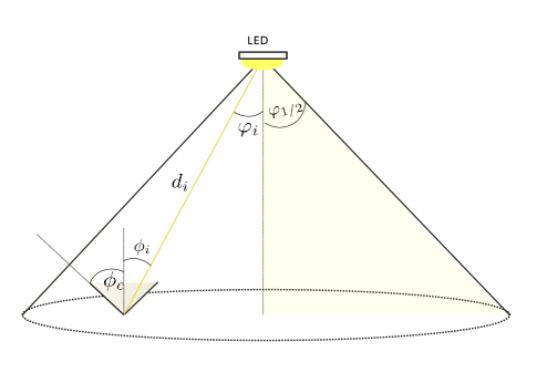
Figure 1: VLC channel model.

$$g(\phi_{i})=\begin{cases}\frac{n^{2}}{\sin^{2}(\phi_{c})},\qquad\qquad&0\leq\phi_{i}\leq\phi_{c}\\ 0,\qquad&\phi_{i}>\phi_{c}\end{cases}$$ (2)

where $n$ denotes the corresponding refractive index. Moreover, $R_{o}(\varphi_{i})$ in (1) is the Lambertian radiant intensity of the transmitting LEDs, which can be expressed as

$$R_{o}(\varphi_{i})=\frac{(m+1)}{2\pi}\cos^{m}(\varphi_{i})$$ (3)

where $m$ is the order of Lambertian emission, calculated as

$$m=\frac{-\ln(2)}{\ln(\cos(\varphi_{1/2}))}$$ (4)

with $\varphi_{1/2}$ denoting the transmitter semi-angle at half power. To this effect, the receiver-site noise is drawn from a circularly-symmetric Gaussian distribution of zero mean and variance

$$\sigma_{n}^{2}=\sigma_{sh}^{2}+\sigma_{th}^{2}$$ (5)

where $\sigma_{sh}^{2}$ and $\sigma_{th}^{2}$ are the variances of the shot noise and thermal noise, respectively.

The shot noise in an optical wireless channel results from the high rate physical photo-electronic conversion process, with variance at the i-th PD

$$\sigma_{sh_{i}}^{2}=2qB\left(\gamma h_{i}x_{j}+I_{bg}I_{2}\right)$$ (6)

where q is the electronic charge, $\gamma$ is the detector responsivity, B is the corresponding bandwidth, $I_{bg}$ is background current, and $I_{2}$ is the noise bandwidth factor. Furthermore, the thermal noise is generated within the transimpedance receiver circuitry and its variance is given by

$$\sigma_{th_{i}}^{2}=\dfrac{8\pi KT_{k}}{G}\eta AI_{2}B^{2}+\dfrac{16\pi^{2}KT_{k}\Gamma}{g_{m}}\eta^{2}A^{2}I_{3}B^{3}$$ (7)

where $K$ is Boltzmann’s constant, $T_{k}$ is the absolute temperature, G is the open-loop voltage gain, A is the PD area, $\eta$ is the fixed capacitance of the PD per unit area, $\Gamma$ is the field-effect transistor (FET) channel noise factor, $g_{m}$ is the FET transconductance, and $I_{3}$ = 0.0868 [39].

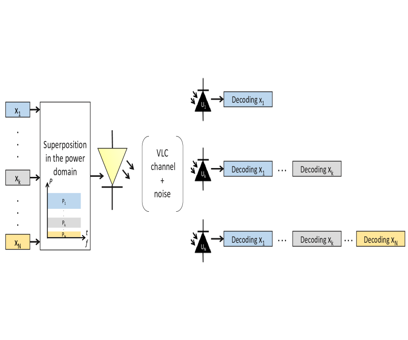
Figure 2: NOMA-VLC downlink.

II-B NOMA Transmission

Without loss of generality, we assume that the users $U_{1}$, …, $U_{N}$ are sorted in an ascending order according to their channels, i.e. $h_{1}\leq h_{2}\leq\cdots\leq h_{N}$. Using NOMA, the LED transmits the real and non-negative signals $s_{1}$, …, $s_{N}$ with associated power values $P_{1}$, …, $P_{N}$, where $s_{i}$ conveys information intended for user $U_{i}$, as shown in Fig. 2. Unless otherwise stated, the term power refers to the optical power which is directly proportional to the LED driving current. To this effect, the $N$ transmitted signals are superimposed in the power domain as follows:

$$x=\sum\limits_{i=1}^{N}P_{i}s_{i}$$ (8)

and the LED total transmit power is $P_{LED}=\sum_{i=1}^{N}P_{i}$. At the PD site, direct detection of the received signal is performed based on the received optical power and the received signal at user $U_{k}$ can be expressed as

$$y_{k}=\gamma h_{k}\sum\limits_{i=1}^{N}P_{i}s_{i}+n_{k}$$ (9)

where $\gamma$ is the detector responsivity and $n_{k}$ denotes zero-mean additive white Gaussian noise (AWGN) with variance $\sigma_{n}^{2}$. Henceforth, $\mathcal{N}(\mu,\sigma^{2})$ represents the probability density function (PDF) of Gaussian distribution with mean $\mu$ and variance $\sigma^{2}$. Based on this and assuming unipolar OOK signals, the PDF of the received signal at $U_{k}$ can be represented as

$$\begin{cases}f_{Y_{k}|S_{k}}(y_{k}|s_{k}=0)=\mathcal{N}_{y_{k}}(\gamma h_{k}\sum\limits_{\begin{subarray}{c}i=1\\ i\neq k\end{subarray}}^{N}P_{i}s_{i},{\sigma_{n}}^{2})\\ f_{Y_{k}|S_{k}}(y_{k}|s_{k}=1)=\mathcal{N}_{y_{k}}(\gamma h_{k}(P_{k}+\sum\limits_{\begin{subarray}{c}i=1\\ i\neq k\end{subarray}}^{N}P_{i}s_{i}),{\sigma_{n}}^{2}).\end{cases}$$ (10)

It is recalled that the multi-user interference at user $U_{k}$ can be eliminated by means of SIC. Based on this, in order to decode its own signal, $U_{k}$ needs to successfully decode and subtract the signals of all other users with lower decoding order, i.e. $s_{1}$, …, $s_{k-1}$. As a result, the residual interference from $s_{k+1},\ldots,s_{N}$ becomes insignificant and can be treated as noise.

In order to facilitate SIC decoding, the LED allocates higher transmission power to users with poor channel gains. The simplest power allocation scheme is the fixed power allocation (FPA), where the associated power of the i-th sorted user is set to

$$P_{i}=\rho P_{i-1}$$ (11)

with $\rho$ denoting the power allocation factor ($0<\rho<1$). According to FPA, the power allocated to user $U_{i}$ is reduced at the increase of $h_{i}$ because users with good channel conditions require lower power levels to successfully decode their desired signals, after canceling the interference from the signals of the users with lower decoding order. This is the fundamental principle of NOMA and has been shown to provide remarkable performance gains in RF-based communications [20].

III NOMA-VLC with perfect CSI

It is recalled that accurate CSI is of paramount importance in conventional and emerging communications as encountered imperfections in practical deployments lead to significant degradation of the overall system performance. This is also the case in VLC; therefore, in this section, we derive a closed form expression for the BER of NOMA-VLC systems employing unipolar OOK under the assumption of perfect knowledge of the channel coefficients and ideal time synchronization.

Theorem 1.

Given that user $U_{k}$ attempts to cancel the first $k-1$ signals from the aggregate received signal in succession, the BER of $U_{k}$ achieved by the NOMA scheme can be written as

$$\mbox{Pr}_{e_{k}}=\sum_{e_{k-1=-1,0,1}}\ldots\sum_{e_{1=-1,0,1}}\mathcal{P}(e_{k-1}|e_{1},\dots,e_{k-2})\enspace\mathcal{P}(e_{k-2}|e_{1},\ldots,e_{k-3})\enspace\cdots\enspace\mathcal{P}(e_{1})\mbox{Pr}_{e_{k}}|e_{1},\ldots,e_{k-1}$$ (12)

It can be inferred from (12) that the probability of error in decoding the $k^{th}$ user signal depends on the detections of the signals $1$ to $k-1$ that are performed during SIC stages. So the probability of error in decoding the $k^{th}$ signal equals the conditional error probability in decoding signal $k$, conditioned on the error probabilities of the previous detection stages $(\mbox{Pr}_{e_{k}}|e_{1},\ldots,e_{k-1})$, multiplied by the error probabilities of all the previous detection stages, where $\mathcal{P}({e_{i}}|{e_{1}},\ldots,{e_{i-1}})$ is the bit-error probability (BEP) of the $i^{th}$ detection stage conditioned on the previous $1$ to $i-1$ BEPs, which is represented as

$$\mathcal{P}({e_{i}}|{e_{1}},\ldots,{e_{i-1}})=\begin{cases}1-{\rm Pr}_{{e_{i}}|{e_{1}},\ldots,{e_{i-1}}}&{e_{i}}=0\\ \frac{1}{2}{\rm Pr}_{{e_{i}}|{e_{1}},\ldots,{e_{i-1}}}&{e_{i}}=-1,1\end{cases}$$

with ${e_{i}}=\hat{s_{j}}-s_{j}$ denoting the error in detecting the i-th OOK signal, and $\mbox{Pr}_{{e_{k}}}|{e_{1}},\ldots,{e_{k-1}}$ is the error probability in decoding the k-th signal conditioned on the previous detections, namely

$$\begin{split}\mbox{Pr}_{{e_{k}}}|{e_{1}},\ldots,{e_{k-1}}=&\frac{1}{2^{N-k+1}}\sum_{i=1}^{2^{N-k}}\mathcal{Q}\left(\frac{\gamma h_{k}}{\sigma_{n}}\left(\frac{P_{k}}{2}-\sum_{j=1}^{k-1}{e_{j}}P_{j}-\sum_{l=k+1}^{N}P_{l}A_{il}\right)\right)\\ &+\frac{1}{2^{N-k+1}}\sum_{i=1}^{2^{N-k}}\mathcal{Q}\left(\frac{\gamma h_{k}}{\sigma_{n}}\left(\frac{P_{k}}{2}+\sum_{j=1}^{k-1}{e_{j}}P_{j}+\sum_{l=k+1}^{N}P_{l}A_{il}\right)\right)\end{split}$$ (13)

where $\mathcal{Q}(x)=\frac{1}{\sqrt{2\pi}}\int_{x}^{\infty}e^{-\frac{y^{2}}{2}}dy$ denotes the one dimensional Gaussian $Q-$function and the term $\sum_{j=1}^{k-1}{e_{j}}P_{j}$ represents the potential residual interference caused by detection error in the decoding of $s_{1}$, …, $s_{k-1}$. Moreover, $\sum_{l=k+1}^{N}P_{l}A_{il}$ corresponds to the interference caused by $s_{k+1}$, …, $s_{N}$, where the elements of the matrix

$$\textbf{A}=\left[\begin{array}[]{ccc}A_{1\enspace k+1}&\dots&A_{1\enspace N}\\ A_{2\enspace k+1}&\dots&A_{2\enspace N}\\ \vdots&\vdots&\vdots\\ A_{2^{N-k}\enspace k+1}&\dots&A_{2^{N-k}\enspace N}\\ \end{array}\right]=\left[\begin{array}[]{cccc}0&0&\dots&0\\ 0&0&\dots&1\\ \vdots&\vdots&\vdots&\vdots\\ 1&1&\dots&1\\ \end{array}\right].$$ (14)

demonstrate the possible combinations of interference depending on the transmitted OOK vectors.

Proof.

The proof is provided in Appendix A. ∎

IV NOMA-VLC with Imperfect CSI

As already mentioned, NOMA configurations are rather sensitive to the knowledge of all users’ channel coefficients. This is of paramount importance not only for successful data recovery at the receivers, but it is also crucial at the transmitter site for determining the power to be allocated to each corresponding user. This is based on the fact that users must receive signals with different power levels, depending on the ordering of their channel gains, in order to effectively facilitate SIC. Thus, while the channel in VLC is technically deterministic for specific transmitter-receiver specifications and fixed locations, the assumption of perfect CSI is not practically realistic even for indoor VLC systems. Typically, CSI can be firstly determined at the receiver site with the aid of periodic pilot signals and then, the receivers feed back the quantized channel coefficients to the transmitters through an RF or infrared (IR) uplink. To this effect, the uncertainty in the VLC channel estimation arises from the noise in the downlink and uplink channels as well as from the mobility of users in indoor environments. Moreover, AD/DA conversion of the channel estimates introduces quantization errors that add to the channel uncertainty, which is beyond the scope of our work [40]. Therefore, it becomes evident that it is essential to quantify the effects of imperfect CSI on the performance of NOMA VLC systems. To this end, we consider two different realistic stochastic uncertainty models for the CSI, namely noisy CSI and outdated CSI.

IV-A Noisy CSI

By assuming that $\hat{h}_{k}$ is the estimate for the channel between the k-th user and the transmitting LED, it follows that

$$\hat{h}_{k}=h_{k}+\epsilon_{n}$$ (15)

where $\epsilon_{n}$ denotes the channel estimation error modeled as a zero-mean Gaussian distribution with variance $\sigma_{\epsilon_{n}}^{2}$, i.e, $\epsilon_{n}\sim\mathcal{N}(0,\sigma_{\epsilon_{n}}^{2})$, which has been adopted as a reasonable model for indoor VLC systems [30, 32]. To this effect, it immediately follows that the channel estimate $\hat{h}_{k}$ can be modelled as $\hat{h}_{k}\sim\mathcal{N}(h_{k},\sigma_{\epsilon_{n}}^{2})$. Under the realistic case of noisy CSI, the conditional error probability for user $U_{k}$ can be approximated by the following Proposition.

Proposition 1.

Under noisy CSI, the error in decoding the k-th signal at $U_{k}$ conditioned on the previous detections is given by

$$\mbox{Pr}_{{e_{k}}}|{e_{1}},\ldots,{e_{k-1}} \approx\frac{1}{2^{N-k+1}\sqrt{\sigma_{\epsilon_{n}}^{2}}}\sum_{i=1}^{2^{N-k}}{\frac{1}{\sqrt{\alpha_{i}}}}e^{c-\frac{\mathcal{P}\left(2a{h_{k}}^{2}\mathcal{P}+b\left(b\mathcal{P}{\sigma_{\epsilon_{n}}}^{2}+2h_{k}{\sigma_{n}}\right)\right)}{4a\mathcal{P}^{2}{\sigma_{\epsilon_{n}}}^{2}-2{\sigma_{n}}^{2}}}$$ (16)

$$+\frac{1}{2^{N-k+1}\sqrt{\sigma_{\epsilon_{n}}^{2}}}\sum_{i=1}^{2^{N-k}}{\frac{1}{\sqrt{\alpha_{i}}}}e^{c-\frac{\tilde{\mathcal{P}}\left(2a{h_{k}}^{2}\tilde{\mathcal{P}}+b\left(b\tilde{\mathcal{P}}{\sigma_{\epsilon_{n}}}^{2}+2h_{k}{\sigma_{n}}\right)\right)}{4a\tilde{\mathcal{P}}^{2}{\sigma_{\epsilon_{n}}}^{2}-2{\sigma_{n}}^{2}}}$$

where

$$\alpha=\frac{1}{{\sigma_{\epsilon_{n}}}^{2}}-\frac{2a\mathcal{P}^{2}}{{\sigma_{n}}^{2}}$$ (17)

and

$$\mathcal{P}=\frac{P_{k}}{2}-\sum_{j=1}^{k-1}{e_{j}}P_{j}-\sum_{l=k+1}^{N}P_{l}A_{il}$$ (18)

while, similarly

$$\tilde{\alpha}=\frac{1}{{\sigma_{\epsilon_{n}}}^{2}}-\frac{2a\tilde{\mathcal{P}}^{2}}{{\sigma_{n}}^{2}}$$ (19)

and

$$\tilde{\mathcal{P}}=\frac{P_{k}}{2}+\sum_{j=1}^{k-1}{e_{j}}P_{j}+\sum_{l=k+1}^{N}P_{l}A_{il}.$$ (20)

Proof.

The proof is provided in Appendix B. ∎

IV-B Outdated CSI

Outdated CSI error may result from the variations in channel realizations due to the mobility of users and/or shadowing effects that occur after the latest channel estimate update. In this context, we consider a deterministically bounded random variable $\epsilon_{o}$ to model the outdated CSI error as

$$\hat{h}_{k}=h_{k}+\epsilon_{o}$$ (21)

where $\epsilon_{o}\leq\mathcal{E}$, with $\mathcal{E}$ denoting the error bound that occurs when the mobile user moves with maximum velocity between the reception of pilot signals and data [32]. In what follows, we derive a tight upper bound for the conditional error probability at user $U_{k}$.

Proposition 2.

The conditional error probability at user $U_{k}$ for the case of outdated CSI can be upper bounded as follows:

$$\mbox{Pr}_{e_{k}}|{e_{1}},\ldots,{e_{k-1}}\leq \frac{1}{2^{N-k+1}}\sum_{i=1}^{2^{N-k}}\mathcal{Q}\left(-\frac{P_{k}}{2{\sigma_{n}}}\mathcal{E}+\frac{\gamma h_{k}}{\sigma_{n}}\left(\frac{P_{k}}{2}-\sum_{j=1}^{k-1}{e_{j}}P_{j}-\sum_{l=k+1}^{N}P_{l}A_{il}\right)\right)$$ (22)

$$+\frac{1}{2^{N-k+1}}\sum_{i=1}^{2^{N-k}}\mathcal{Q}\left(-\frac{P_{k}}{2{\sigma_{n}}}\mathcal{E}+\frac{\gamma h_{k}}{\sigma_{n}}\left(\frac{P_{k}}{2}+\sum_{j=1}^{k-1}{e_{j}}P_{j}+\sum_{l=k+1}^{N}P_{l}A_{il}\right)\right).$$

Proof.

The proof is provided in Appendix C. ∎

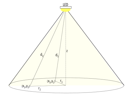
Figure 3: Outdated CSI resulting from user mobility.

IV-B1 Determination of the value of $\mathcal{E}$

In order to obtain the upper bound on the CSI error, we simplify the channel gain by substituting (2) and (3) into (1) and substituting $\cos\varphi_{i}$ with $z/d_{i}$, where $z$ denotes the height between the LEDs and the PDs, which is assumed to be fixed, i.e., at a level of an ordinary table. Based on this and by assuming vertical alignment of LEDs and PDs, the corresponding channel gain $h_{i}$ can be expressed as

$$h_{i}=\varpi\frac{1}{d^{m+3}_{i}}$$ (23)

where

$$\varpi=\frac{(m+1)A_{i}T_{s}(\phi_{i})g(\phi_{i})}{2\pi}.$$ (24)

By now referring to Fig. 3, let user $U_{k}$ move in the horizontal plane from $(x_{1},y_{1})$ to $(x_{2},y_{2})$ with maximum velocity $v$. Then, the error bound $\mathcal{E}$ can be calculated as follows

$$\mathcal{E}=\varpi|{d^{m+3}_{2}}-{d^{m+3}_{1}}|$$ (25)

where $d^{2}_{1}=r^{2}_{1}+z^{2}$, $d^{2}_{2}=r^{2}_{2}+z^{2}$, and $v=\sqrt{r^{2}_{1}-r^{2}_{2}}/t$, with $t$ denoting the time elapsed since the last CSI update. It is evident that the algebraic representation of (25) is tractable and can be computed straightforwardly. Furthermore, it is particularly accurate, as shown in detail in Section VI.

V NOMA-VLC with Dimming Control

In this Section, we investigate the performance of NOMA-VLC under dimming control. To this end, it is firstly recalled that adjusting the brightness level of the LED can be achieved by two approaches: 1) analog dimming, where the driving current of the LED is directly adjusted to the required illumination level; 2) digital dimming, in which the driving current is maintained constant while the duty cycle is varied in order to acquire the desired brightness [41, 42]. Therefore, analog dimming is straightforward to implement given that the LED brightness is directly proportional to the forward current. However, this technique may cause chromaticity shift problems as it alters the transmitted wavelength. To implement analog dimming, we use unipolar OOK signal to drive the LED and dimming is achieved by altering the driving current to match the dimming target. In this context, the driving current, and, consequently, the transmitted optical power, are set to be proportional to the dimming factor $\gamma_{d}$. In this case, the error in decoding the k-th signal conditioned on the previous detections can be obtained by (13), (16) and (22) for perfect, noisy and outdated CSI, respectively by changing the transmit power from $P$ to $\gamma_{d}P$.

On the contrary, digital dimming imposes a pulse width modulation (PWM) signal with a duty cycle that is determined by the required dimming factor. This technique alleviates the chromaticity shifts, but at a cost of reduced spectral efficiency. In the present analysis, we implement digital dimming by means of VOOK as in [35], where the brightness of the LED is controlled by adopting the data duty cycle $\delta_{d}$ of the OOK signal. Based on this, information bits are transmitted when the duty cycle is on, while the off portion is filled with dummy bits that are either zeros or ones, depending on the dimming factor $\gamma_{d}$. VOOK codewords are depicted in Table I, indicating that when $\gamma_{d}=0$, the lights are completely turned off while when $\gamma_{d}=1$, full brightness is achieved. Accordingly, no data bits are transmitted when $\gamma_{d}$ is set to $0$ or $1$. To this effect, with the use of coded VOOK, the BER in decoding the k-th signal conditioned on the previous k-1 detections can be expressed as follows

$$\mbox{Pr}_{e_{k}VOOK}|{e_{1}},\ldots,{e_{k-1}}=\sum_{\lceil i=n/2\rceil}^{n}\binom{n}{i}{\mbox{Pr}^{i}_{e_{k}|{e_{1}},\ldots,{e_{k-1}}}}(1-\mbox{Pr}_{e_{k}|{e_{1}},\ldots,{e_{k-1}}})^{n-i}$$ (26)

where $\mbox{Pr}_{e_{k}|{e_{1}},\ldots,{e_{k-1}}}$ can be obtained from (13), (16) and (22) for perfect, noisy and outdated CSI respectively, and $n$ is the number of redundant bits in the VOOK codewords, calculated as

$$n=\begin{cases}20\gamma_{d},\qquad&0<\gamma_{d}\leq\frac{1}{2}\\ 20-20\gamma_{d},\qquad&\frac{1}{2}\leq\gamma_{d}<1.\end{cases}$$ (27)

It is noted that the use of redundant bits in VOOK leads to BER improvements as $n$ increases, yet, digital dimming affects the system spectral efficiency as the achievable data rate deteriorates lineally with the number of bits in the corresponding codewords.

TABLE I: VOOK Codewors

$\gamma_{d}$	$\delta_{d}$	VOOK Codeword
1.0	$1.0$	1111111111
0.9	$0.2$	dd11111111
0.8	$0.4$	dddd111111
0.7	$0.6$	dddddd1111
0.6	$0.8$	dddddddd11
0.5	$1.0$	dddddddddd
0.4	$0.8$	dddddddd00
0.3	$0.6$	dddddd0000
0.2	$0.4$	dddd000000
0.1	$0.2$	dd00000000
0.0	$0.0$	0000000000

VI Results and Discussion

In this section, we employ the derived analytic expressions in the analysis of the considered setups. Respective results from extensive Monte Carlo simulations are also provided to verify the validity and usefulness of the offered results. Thus, the BER performance of a NOMA-VLC downlink system is analyzed for different scenarios based on the system and channel models in Section II. It should be noted here that the considered channel model is independent of the room geometry, To this end and without loss of generality, we consider that the users exist within a $4m\times 4m\times 3m=48m^{3}$ room environment.

We consider one transmitting LED mounted at the centre of the ceiling and, in order to ensure comparability, fixed LED transmitting power is used in all scenarios. We also assume the existence of three users in the coverage area of the transmitting LED that are planned to be served simultaneously using NOMA. It is emphasized here that this number of users is selected for indicative purposes and that the considered system model is generic and applicable to any number of users. In this context, the LED superimposes the signals of the three users in the power domain by allocating the power values $P_{1}$, $P_{2}$ and $P_{3}$ to $U_{1}$, $U_{2}$ and $U_{3}$ respectively, under the constraint $P_{1}+P_{2}+P_{3}=P_{\rm LED}$. In the used notation, $U_{i}$ denotes the user in i-th decoding order; that is, $h_{i}$ is in the i-th ascending order of the channel gains. The channel gains of all users along with other system parameters are depicted in Table II. For the results that involve users’ mobility, the locations of the users are randomly generated. It should be noted here that the underlying symmetry in VLC systems may lead to similar channel gains and, consequently, resulting to a higher error rate. This issue was addressed in an earlier work [18], where we proposed a strategy based on tuning the FOVs of the receiving PDs in order to maximize the differences between the channel gains and improve the performance of NOMA.

(a)

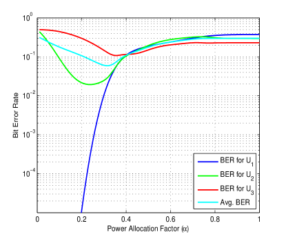
(b)

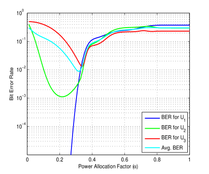
(c)

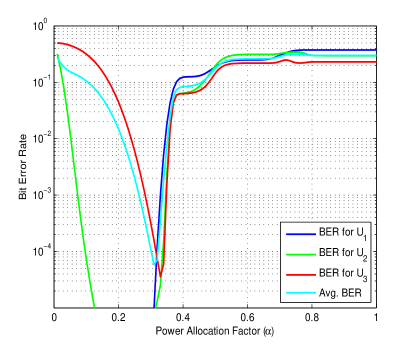
Figure 4: BER performance under fixed power allocation (a) SNR=110 dB, (b) SNR=115 dB and (c) SNR=120 dB.

TABLE II: Simulation Parameters

Description	Notation	Value
LED power	$P_{\rm LED}$	0.25 W
Transmitter semi-angle	$\varphi_{i}$	$50$ deg
FOV of the PDs	$\phi_{c_{i}}$	$45$ deg
Physical area of PD	$A_{i}$	$1.0$ ${\rm cm^{2}}$
Refractive index of PD lens	$n$	$1.5$
Gain of optical filter	$T_{s}(\phi_{li})$	$1.0$
Data rate	$B$	$10$ ${\rm Mbps}$
Total number of users	$N$	3
Channel gain of $U_{1}$	$h_{1}$	$0.2835\times 10^{-4}$
Channel gain of $U_{2}$	$h_{2}$	$0.4787\times 10^{-4}$
Channel gain of $U_{3}$	$h_{3}$	$0.5272\times 10^{-4}$

We evaluate the BER performance with regard to the transmit SNR in order to include the individual path gain of each user. Since the channel gain is in the order of $10^{-4}$, the corresponding results exhibit an offset of about $80$ dB with respect to the SNR at the receiver site. First, we investigate the effect of the power allocation factor $\rho$ in (11) on the BER performance under fixed power allocation. To this end, Fig. 4 shows the average BER and the individual BER for the three users versus $\rho$ for different transmit SNR values of $110$ dB, $115$ dB and $120$ dB. It is shown that, despite its poor channel conditions, the user in the first decoding order, i.e., $U_{1}$, provide comparable error performance to other users. This is because the signal intended for this user is transmitted with a high power compared to other signals, in order to enable $U_{1}$ to directly decode its signal of interest regardless of the interference it receives. Moreover, the best average BER performance for all users can be achieved at about $\rho=0.3$, as in this value, the power levels allocated to users experiencing low channel gains are sufficiently high to enable correct signal decoding. As $\rho$ increases, users with good channel conditions receive with higher power levels, which in turn reduces the power associated with the signals of the other users. As a consequence, high errors occur in the early stages of SIC decoding, and are then inherited to the following stages, which ultimately leads to poor BER performance. For the rest of the results in this Section, $\rho=0.3$ is considered.

The BER expression derived in Section III is validated by Fig. 5, which shows the BER performance of the three users assuming perfect CSI. It is shown that the derived analytic results are in excellent agreement with the respective Monte Carlo simulation results. It is evident that the user with the lowest decoding order exhibits the best BER performance, while the performance degrades as the decoding order increases. Yet, all users exhibit satisfactory performance above transmit SNR of $120$ dB that corresponds to receive SNR of about $40$ dB, which is a typical range in VLC transmissions.

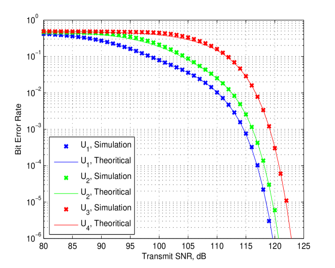
Figure 5: BER Performance with Perfect CSI.

In the following, we investigate the effect of channel uncertainty on the performance of NOMA-VLC. To this end, we assume that the uplink to the LED is error free, so that the LED and the users have the same estimates of the channel gains. For the case of noisy CSI, two different models are used: 1) fixed error variance, where $\sigma_{\epsilon_{n}}^{2}$ is independent of the transmit SNR; 2) varying error variance, where $\sigma_{\epsilon_{n}}^{2}$ is a decreasing function of the transmit SNR. Furthermore, we assume that the noisy channel error variances are identical at the different users. In order to obtain an insight on the impact of different CSI variances on system performance, Fig. 6 illustrates the BER performance versus different fixed values of $\sigma_{\epsilon_{n}}^{2}$ at a transmit SNR of $115$ dB. It is clear that users with lower decoding order suffer from higher errors due to the involved channel uncertainty. This is particularly evident at user $U_{1}$ that exhibits substantial BER degradation compared to the error-free CSI (indicated by dashed line). The reason is that $U_{1}$ has the lowest channel gain among all users, which renders signal detection highly sensitive to errors in the available CSI. Moreover, $U_{1}$ needs to decode $x_{1}$ with the existence of high interference from the signals of other users, which increases the severity of the effect of imperfect CSI. Furthermore, although other users also need to decode $x_{1}$ despite the involved interference, their relatively high channel gains make the detection more robust to channel errors from the early stages of the detection. This is specifically clear for $U_{3}$ that is the least affected by channel uncertainty. It should be noted here that the CSI error resulting from the noisy channel is in general small enough not to affect the ordering of channel gains. Hence, the power allocation based on CSI available at the transmitter is not ultimately affected. Fig. 7 demonstrates the corresponding BER performance under fixed and SNR-dependant error variances. It is observed that fixed $\sigma_{\epsilon_{n}}^{2}$ results to an irreducible error floor at high SNRs for users with low decoding order. However, when $\sigma_{\epsilon_{n}}^{2}$ is modeled as SNR-dependant, the BER decreases with the increase in transmit SNR. It is not surprising to observe that the performance of user $U_{3}$ is almost the same for the two variance models, which is due to the fact that the impact of error is already insignificant at this user. In order to validate the BER expression for noisy CSI in Proposition 1, we plot the BER performance with the aid of the derived approximation along with respective results from Monte Carlo simulations in Fig. 8. It is observed that, the derived approximation provides accurate results that are in tight agreement with the simulation results. Moreover, it is noted that the user in the first decoding order suffers higher performance degradation compared to users with higher decoding orders. This is due to the fact that $U_{1}$ does not perform SIC, which means that it has to deal with the existing interference along with the CSI error. Moreover, $U_{1}$ has the lowest channel gain among all users, which makes the effect of noisy CSI rather detrimental.

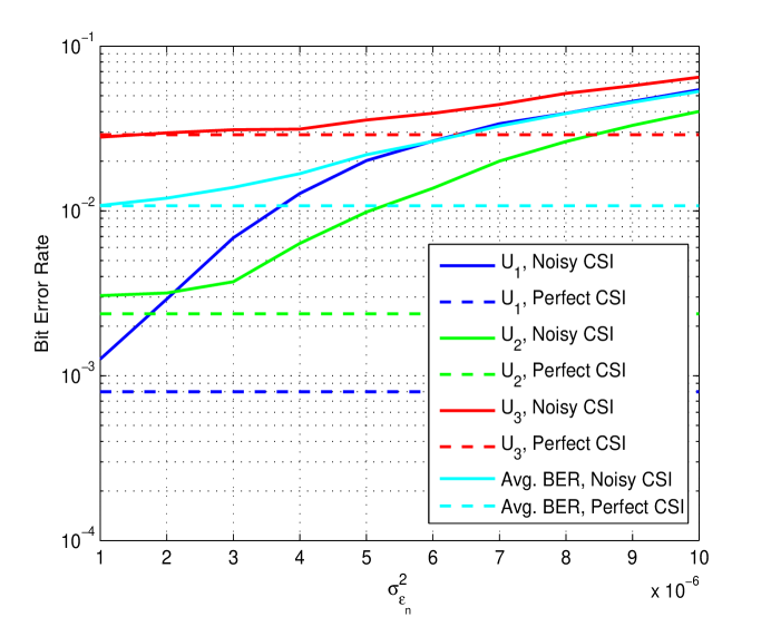
Figure 6: BER Performance for different values of $\sigma_{\epsilon_{n}}^{2}$.

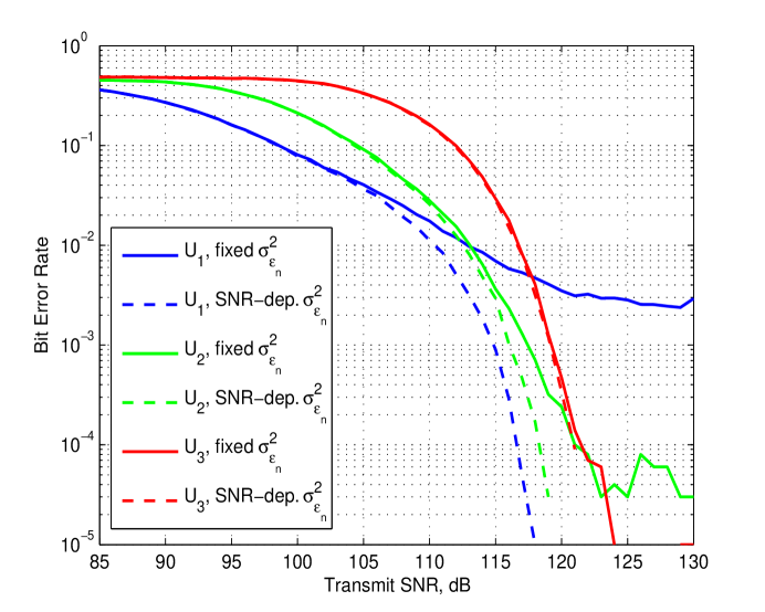
Figure 7: BER Performance with Noisy CSI, for fixed and SNR-dependent error variances.

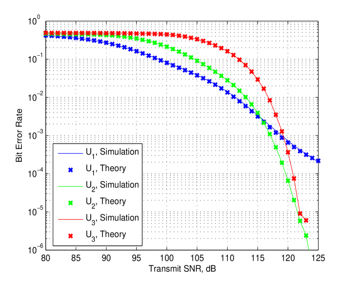
Figure 8: BER Performance with Noisy CSI, $\sigma_{\epsilon_{n}}^{2}=2\times 10^{-6}$ .

Next, we quantify the effect of the mobility of the indoor users. To this end, it is recalled that VLC channels are mainly dependant upon the user location with respect to the transmitting LED. As a result, even a slight change in the user’s location results in a change of the corresponding channel gain. To this effect, if a user possesses an outdated channel estimation, i.e., a change of location occurs before the next channel update, CSI becomes erroneous. In order to quantify the impact of outdated CSI on the overall system performance, we simulate the mobility of indoor users with random speed from $0$ to $2$ m/s while they remain connected to the same LED. We then assume that the change in location may occur between CSI updates and thus, both transmitter and receiver use the outdated CSI for power allocation and decoding, respectively. It is also noted here that outdated CSI, unlike noisy CSI, may lead to a change in the ordering of the channel gains of the users which ultimately leads to unfair power allocation at the transmitter, where high power values may be allocated to users with good channel conditions and vice versa. This results to a dramatic performance degradation for users with poor channel gains, as their allocated power becomes insufficient for successful decoding. In the same context, Fig. 9 and Fig. 10 demonstrate the BER performance with outdated CSI for the three users, where the upper bound for the error is determined by (22), in Proposition 2, when the user moves with maximum velocity. In Fig. 9, we simulate the mobility of users assuming that their relative channel ordering remains constant, which is valid if users change locations in the same trend, i.e. Reference Point Group Model [45], which is realistic in large indoor environments, such as museums or airports. On the contrary, Fig. 10 illustrates the performance degradation caused by unfair power allocation when outdated CSI leads to change in the ordering of users’ gains. It is noted that for the sake of consistency with other figures, $U_{1}$ here denotes the user that has the lowest channel gain among all users. However, $U_{1}$ now is not in the first decoding order as its channel is erroneously estimated not to be the lowest. Therefore, users with low channel gains suffer, as expected, from dramatic degradation, while $U_{3}$ benefits from the high power that is in fact erroneously allocated to it. As a consequence, the high power allows $U_{3}$ to detect the desired signal effectively, even though the estimate of $h$ available at the decoder is practically inaccurate.

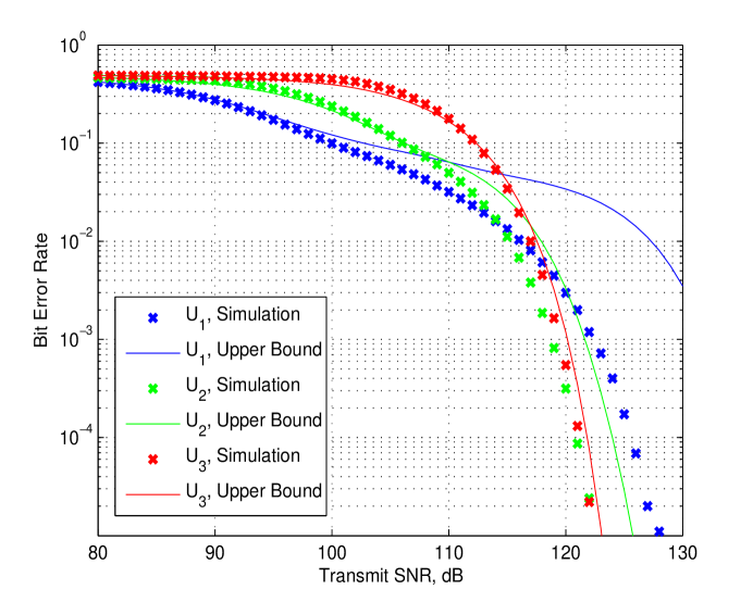
Figure 9: BER Performance with Outdated CSI, order not changed.

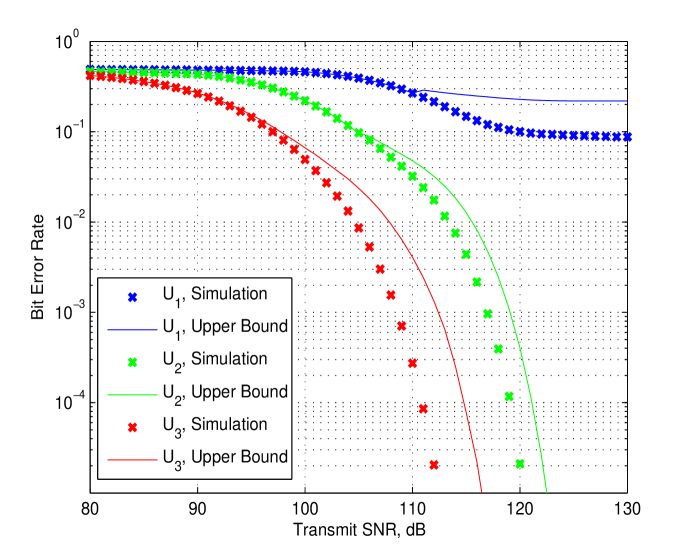
Figure 10: BER Performance with Outdated CSI, order changed.

Finally, we evaluate the BER performance of the NOMA-VLC system under dimming control. Fig. 11 and Fig. 12 demonstrate the BER of the three users under analog and digital dimming schemes, respectively. As expected, analog intensity dimming leads to BER performance degradation, particularly at low $\gamma_{d}$ values, as lower transmit power is used, which reduces the received SNR. On the contrary, digital dimming employed by means of VOOK leads to BER enhancement, that is substantial when the dimming factor is around $0.5$. This is achieved thanks to the increase of redundant data bits, which in turn reduces the probability of incorrect detections. Yet, this enhancement comes at the cost of reduction in the achievable throughput, which is the main drive for NOMA. The effect of imperfect CSI under dimming is also demonstrated, which indicates that outdated CSI leads to higher performance degradation compared to noisy CSI, which is in agreement with the previous results.

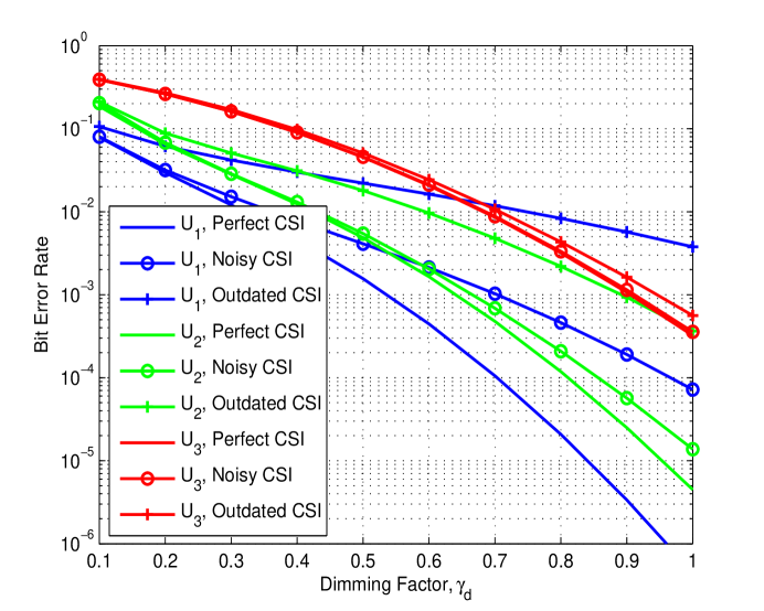
Figure 11: BER Performance with analog intensity dimming.

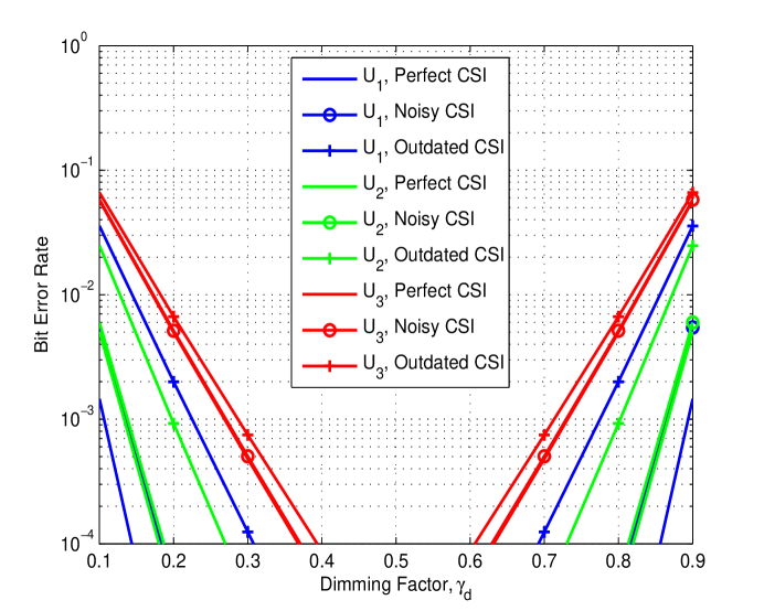
Figure 12: BER Performance with digital VOOK dimming.

VII Conclusions

This work was devoted to the analysis of the BER performance in a downlink VLC network where multiple access was provided by means of NOMA. This was realized for the case of both perfect and imperfect CSI, which showed that noisy CSI leads to, as expected, a degradation of the system performance. However, this degradation is rather smaller compared to the one created by outdated CSI which results from the mobility of the user terminal between two CSI updates and cause detrimental performance loss if the ordering of the users’ channel gains change between the channel updates. The validity of the derived analytic results was justified by extensive comparisons with results from respective Monte Carlo simulations. Finally, the offered results provided meaningful insights that are expected to be useful in future design and deployments of VLC systems.

Appendix A Proof of Theorem 1

Using maximum-likelihood (ML) detector, the decoder at the k-th receiver decides for the vector $\hat{s}$ that minimizes the Euclidean distance between the received signal vector $y$ and the potential received signals leading to

$$\hat{{s}}=\mbox{arg}\min\limits_{s}\left|{y-\gamma h_{k}s}\right|^{2}.$$ (28)

Based on this and assuming that the $U_{k}$ user cancels successfully the signals $s_{1}$ , …, $s_{m-1}$, the error probability at $U_{k}$ in detecting the signal $s_{m}$ intended to user $U_{m}$ $(1\leq m\leq k-1)$ can be expressed as follows: when the transmitted symbol $s_{m}=0$, the conditional error probability is given by

$$\mbox{Pr}_{e_{m\rightarrow k|s_{m}=0}}=\int_{\frac{1}{2}\gamma h_{k}P_{m}}^{\infty}\mathcal{N}_{y_{k}}\left(\gamma h_{k}\sum\limits_{i=m+1}^{N}P_{i}s_{i},\sigma_{n}\right)dy_{k}$$ (29)

which can be expressed in closed-form in terms of the $Q-$function, namely

$$\mbox{Pr}_{e_{m\rightarrow k|s_{m}=0}}=\mathcal{Q}\left(\frac{\gamma h_{k}}{\sigma_{n}}\left(\frac{P_{m}}{2}-\sum\limits_{i=m+1}^{N}P_{i}s_{i}\right)\right).$$ (30)

On the contrary, when $s_{m}=1$ is transmitted, it follows that

$$\mbox{Pr}_{e_{m\rightarrow k|s_{m}=1}}=\int_{-\infty}^{\frac{1}{2}\gamma h_{k}P_{m}}\mathcal{N}_{y_{k}}\left(\gamma h_{k}\left(P_{m}+\sum\limits_{i=m+1}^{N}P_{i}s_{i}\right),\sigma_{n}\right)dy_{k}$$ (31)

which after some algebraic manipulations, it can be expressed by the following closed-form expression

$$\mbox{Pr}_{e_{m\rightarrow k|s_{m}=1}}=1-\mathcal{Q}\left(\frac{\gamma h_{k}}{\sigma_{n}}\left(-\frac{P_{m}}{2}-\sum\limits_{i=m+1}^{N}P_{i}s_{i}\right)\right)$$ (32)

which with the aid of the identity $Q(-x)=1-Q(x)$ can be equivalently re-written as follows:

$$\mbox{Pr}_{e_{m\rightarrow k|s_{m}=1}}=\mathcal{Q}\left(\frac{\gamma h_{k}}{\sigma_{n}}\left(\frac{P_{m}}{2}+\sum\limits_{i=m+1}^{N}P_{i}s_{i}\right)\right).$$ (33)

It is noted that the above expressions assume perfect cancelation of the first $m-1$ signals. Nevertheless, detection errors may practically occur in any step of the successive cancelation process. Therefore, considering the contribution of the residual interference inherited by cancelation errors, equations (30)-(31) can be alternatively re-written as

$$\mbox{Pr}_{e_{m\rightarrow k|s_{m}=0}} =\int_{\frac{1}{2}\gamma h_{k}P_{m}}^{\infty}\mathcal{N}_{y_{k}}\left(\gamma h_{k}\left(\sum_{j=1}^{m-1}{e_{j}}P_{j}+\sum\limits_{i=m+1}^{N}P_{i}s_{i}\right),\sigma_{n}\right)dy_{k}$$ (34)

$$=\mathcal{Q}\left(\frac{\gamma h_{k}}{\sigma_{n}}\left(\frac{P_{m}}{2}-\sum_{j=1}^{m-1}{e_{j}}P_{j}-\sum\limits_{i=m+1}^{N}P_{i}s_{i}\right)\right)$$

and

$$\mbox{Pr}_{e_{m\rightarrow k|s_{m}=1}} =\int_{-\infty}^{\frac{1}{2}\gamma h_{k}P_{m}}\mathcal{N}_{y_{k}}\left(\gamma h_{k}\left(P_{m}+\sum_{j=1}^{m-1}{e_{j}}P_{j}+\sum\limits_{i=m+1}^{N}P_{i}s_{i}\right),\sigma_{n}\right)dy_{k}$$ (35)

$$=\mathcal{Q}\left(\frac{\gamma h_{k}}{\sigma_{n}}\left(\frac{P_{m}}{2}+\sum_{j=1}^{m-1}{e_{j}}P_{j}+\sum\limits_{i=m+1}^{N}P_{i}s_{i}\right)\right)$$

respectively. Based on the above, the total error probability in decoding $s_{k}$ at $U_{k}$ can be finally obtained by summing up all conditional error probabilities of the previous detections, which completes the proof.

Appendix B Proof of Proposition 1

According to (15), the ML decision rule at user $U_{k}$ is readily expressed as

$$\hat{{s}}=\mbox{arg}\min\limits_{s}\left|{y-\gamma\hat{h}_{k}s}\right|^{2}.$$ (36)

To this effect, the error probability at $U_{k}$ in detecting the signal $s_{m}$ intended to user $U_{m}$ $(1\leq m\leq k-1)$ can be represented as follows:

$$\mbox{Pr}_{e_{m\rightarrow k|s_{k}=0}}=\int_{\frac{1}{2}\gamma P_{m}\hat{h}_{k}}^{\infty}\mathcal{N}_{y_{k}}\left(\gamma h_{k}\left(\sum_{j=1}^{m-1}{e_{j}}P_{j}+\sum\limits_{i=m+1}^{N}P_{i}s_{i}\right),\sigma_{n}\right)dy_{k}$$ (37)

and

$$\mbox{Pr}_{e_{m\rightarrow k|s_{k}=1}}=\int_{-\infty}^{\frac{1}{2}\gamma P_{m}\hat{h}_{k}}\mathcal{N}_{y_{k}}\left(\gamma h_{k}\left(P_{m}+\sum_{j=1}^{m-1}{e_{j}}P_{j}+\sum\limits_{i=m+1}^{N}P_{i}s_{i}\right),\sigma_{n}\right)dy_{k}$$ (38)

where ${e_{j}}=\hat{s_{j}}-s_{j}$. Based on this, and after some algebraic manipulations, the conditional error probability in (13) becomes

$$\mbox{Pr}_{e_{k}}|{e_{1}},\ldots,{e_{k-1}} =\frac{1}{2^{N-k+1}}\int_{-\infty}^{\infty}\Bigg{(}\sum_{i=1}^{2^{N-k}}\mathcal{Q}\bigg{(}\frac{\gamma P_{k}\epsilon_{n}}{2\sigma_{n}}+\frac{\gamma h_{k}}{\sigma_{n}}(\frac{P_{k}}{2}-\sum_{j=1}^{k-1}{e_{j}}P_{j}-\sum_{l=k+1}^{N}P_{l}A_{il})\bigg{)}$$ (39)

$$+\sum_{i=1}^{2^{N-k}}\mathcal{Q}\bigg{(}\frac{-\gamma P_{k}\epsilon_{n}}{2\sigma_{n}}+\frac{\gamma h_{k}}{\sigma_{n}}(\frac{P_{k}}{2}+\sum_{j=1}^{k-1}{e_{j}}P_{j}+\sum_{l=k+1}^{N}P_{l}A_{il})\bigg{)}\Bigg{)}\times\mathcal{N}_{\epsilon_{n}}(0,\sigma_{\epsilon_{n}}^{2})dh_{k}.$$

It is evident that the derivation of an exact closed-form expression to (39) is subject to analytic evaluation of the involved two integrals. However, this is unfortunately not feasible as these integrals are not available in the open technical literature and in tabulated form. Yet, a relatively simple closed-form approximation can be derived instead, which appears to be particularly accurate for all values of the considered scenario. To this end, it is recalled that the one dimensional Gaussian $Q$-function can be accurately expressed by an accurate approximation in [46], namely

$$\mathcal{Q}(x)\approx e^{ax^{2}+bx+c}, \qquad x\geq 0$$ (40)

where $a,b,c\in\mathbb{R}$ are the corresponding fitting parameters that are selected according to the fitting criteria. These values are available in [46] and ensure increased tightness as the corresponding involved absolute and relative errors between the exact and approximated values are particularly small for the entire range of values of $x$. To this effect, by performing the necessary variable transformation in (40) and substituting in (39), one obtains the closed-form expression in (16), which completes the proof.

Appendix C Proof of Proposition 2

Using ML detection, it follows that

$$\mbox{Pr}_{e_{m\rightarrow k|s_{k}=0}}=\int_{\frac{1}{2}\gamma P_{m}\hat{h}_{k}}^{\infty}\mathcal{N}_{y_{k}}\left(\gamma h_{k}\left(\sum_{j=1}^{m-1}{e_{j}}P_{j}+\sum\limits_{i=m+1}^{N}P_{i}s_{i}\right),\sigma_{n}\right)dy_{k}.$$ (41)

The above integral representation can also be expressed in closed-form in terms of the $Q-$function. Based on this, it immediately follows that

$$\mbox{Pr}_{e_{m\rightarrow k|s_{k}=0}}=\mathcal{Q}\left(\frac{1}{\sigma_{n}}\left(\gamma\hat{h}_{k}\frac{P_{m}}{2}-\sum_{j=1}^{m-1}\gamma h_{k}{e_{j}}P_{j}-\sum\limits_{i=m+1}^{N}\gamma h_{k}P_{i}s_{i}\right)\right)$$ (42)

which can be equivalently expressed as

$$\mbox{Pr}_{e_{m\rightarrow k|s_{k}=0}}=\mathcal{Q}\left(\frac{\gamma P_{m}}{2{\sigma_{n}}}\mathcal{E}+\frac{\gamma h_{k}}{\sigma_{n}}\left(\frac{P_{m}}{2}-\sum_{j=1}^{m-1}{e_{j}}P_{j}-\sum_{l=m+1}^{N}P_{l}A_{il}\right)\right).$$ (43)

Likewise,

$$\mbox{Pr}_{e_{m\rightarrow k|s_{k}=1}}=\int_{-\infty}^{\frac{1}{2}P_{m}\gamma\hat{h_{k}}}\mathcal{N}_{y_{k}}\left(\gamma h_{k}\left(P_{m}+\sum_{j=1}^{m-1}{e_{j}}P_{j}+\sum\limits_{i=m+1}^{N}P_{i}s_{i}\right)\sigma_{n}\right)dy_{k}$$ (44)

which can be expressed in closed-form as

$$\mbox{Pr}_{e_{m\rightarrow k|s_{k}=1}}=1-\mathcal{Q}\left(\frac{1}{\sigma_{n}}\left(\gamma\hat{h}_{k}\frac{P_{m}}{2}-\gamma h_{k}P_{m}-\sum_{j=1}^{m-1}\gamma h_{k}{e_{j}}P_{j}-\sum\limits_{i=m+1}^{N}\gamma h_{k}P_{i}s_{i}\right)\right)$$ (45)

and

$$\mbox{Pr}_{e_{m\rightarrow k|s_{k}=1}}=\mathcal{Q}\left(-\frac{\gamma P_{m}}{2{\sigma_{n}}}\mathcal{E}+\frac{\gamma h_{k}}{\sigma_{n}}\left(\frac{P_{m}}{2}+\sum_{j=1}^{m-1}{e_{j}}P_{j}+\sum_{l=m+1}^{N}P_{l}A_{il}\right)\right)$$ (46)

where ${e_{j}}=\hat{s_{j}}-s_{j}$. Based on this and after carrying out some algebraic manipulations, equation (22) is deduced, which completes the proof.

References

- [1] H. Burchardt, N. Serafimovski, D. Tsonev, S. Videv, and H. Haas, “VLC: Beyond point-to-point communication,” IEEE Commun. Mag, vol. 52, no. 7, pp. 98–105, July 2014.
- [2] S. Dimitrov and H. Haas, Principles of LED Light Communications: Towards Networked Li-Fi. Cambridge University Press, 2015.
- [3] A. Jovicic, J. Li, and T. Richardson, “Visible light communication: opportunities, challenges and the path to market,” IEEE Commun. Mag., vol. 51, no. 12, pp. 26–32, December 2013.
- [4] H. Haas, L. Yin, Y. Wang, and C. Chen, “What is LiFi?” J. Lightw. Technol., vol. 34, no. 6, pp. 1533–1544, Mar. 2016.
- [5] D. Karunatilaka, F. Zafar, V. Kalavally, and R. Parthiban, “LED based indoor visible light communications: State of the art,” Commun. Surveys Tuts., vol. 17, no. 3, pp. 1649–1678, Aug. 2015.
- [6] S. Rajbhandari, H. Chun, G. Faulkner, K. Cameron, A. V. N. Jalajakumari, R. Henderson, D. Tsonev, M. Ijaz, Z. Chen, H. Haas, E. Xie, J. J. D. McKendry, J. Herrnsdorf, E. Gu, M. D. Dawson, and D. O’Brien, “High-speed integrated visible light communication system: Device constraints and design considerations,” IEEE J. Sel. Areas Commun., vol. 33, no. 9, pp. 1750–1757, Sep. 2015.
- [7] E. Sarbazi and M. Uysal, “PHY layer performance evaluation of the IEEE 802.15.7 visible light communication standard,” in Proc. 2nd International Workshop on Optical Wireless Communications (IWOW), Oct. 2013, pp. 35–39.
- [8] P. H. Pathak, X. Feng, P. Hu, and P. Mohapatra, “Visible light communication, networking, and sensing: A survey, potential and challenges,” Commun. Surveys Tuts., vol. 17, no. 4, pp. 2047–2077, Fourthquarter 2015.
- [9] S. K. Nobar, K. A. Mehr, and J. M. Niya, “Comprehensive performance analysis of IEEE 802.15.7 CSMA/CA mechanism for saturated traffic,” IEEE J. Opt. Commun. Netw., vol. 7, no. 2, pp. 62–73, Feb. 2015.
- [10] Z. Zhang, X. Yu, L. Wu, J. Dang, and V. O. K. Li, “Performance analysis of full-duplex visible light communication networks,” in Proc. IEEE International Conference on Communications (ICC), June 2015, pp. 3933–3938.
- [11] L. Zhao, X. Chi, and W. Shi, “A QoS-driven random access algorithm for MPR-capable VLC system,” IEEE Commun. Lett, vol. 20, no. 6, pp. 1239–1242, June 2016.
- [12] J. Dang and Z. Zhang, “Comparison of optical OFDM-IDMA and optical OFDMA for uplink visible light communications,” in Proc. International Conference on Wireless Communications Signal Processing (WCSP), Oct. 2012, pp. 1–6.
- [13] J. A. Salehi, “Code division multiple-access techniques in optical fiber networks. I. fundamental principles,” IEEE Trans. Commun., vol. 37, no. 8, pp. 824–833, Aug. 1989.
- [14] J. A. Salehi and C. A. Brackett, “Code division multiple-access techniques in optical fiber networks. II. systems performance analysis,” IEEE Trans. Commun., vol. 37, no. 8, pp. 834–842, Aug. 1989.
- [15] M. Guerra-Medina, B. Rojas-Guillama, O. Gonzalez, J. Martin-Gonzalez, E. Poves, and F. Lopez-Hernandez, “Experimental optical code-division multiple access system for visible light communications,” in Proc. Wireless Telecommunications Symposium (WTS), Apr. 2011, pp. 1–6.
- [16] P. V. Kumar, R. Omrani, J. Touch, A. E. Willner, and P. Saghari, “CTH01-5: A novel optical CDMA modulation scheme: Code cycle modulation,” in Proc. IEEE Globecom, Nov. 2006, pp. 1–5.
- [17] M. F. Guerra-Medina, O. Gonzalez, B. Rojas-Guillama, J. A. Martin-Gonzalez, F. Delgado, and J. Rabadan, “Ethernet-OCDMA system for multi-user visible light communications,” Electronics Letters, vol. 48, no. 4, pp. 227–228, Feb. 2012.
- [18] H. Marshoud, V. M. Kapinas, G. K. Karagiannidis, and S. Muhaidat, “Non-orthogonal multiple access for visible light communications,” IEEE Photon. Technol. Lett., vol. 28, no. 1, pp. 51–54, Jan. 2016.
- [19] NTT DOCOMO Inc., Tokyo, Japan, “5G radio access: requirements, concept and technologies,” 5G Whitepaper.
- [20] L. Dai, B. Wang, Y. Yuan, S. Han, C. l. I, and Z. Wang, “Non-orthogonal multiple access for 5G: solutions, challenges, opportunities, and future research trends,” IEEE Commun. Mag., vol. 53, no. 9, pp. 74–81, Sep. 2015.
- [21] Z. Ding, Z. Yang, P. Fan, and H. Poor, “On the performance of non-orthogonal multiple access in G systems with randomly deployed users,” IEEE Signal Process. Lett., vol. 21, no. 12, pp. 1501–1505, Dec. 2014.
- [22] J. Men and J. Ge, “Non-orthogonal multiple access for multiple-antenna relaying networks,” IEEE Commun. Lett, vol. 19, no. 10, pp. 1686–1689, Oct. 2015.
- [23] Z. Ding, F. Adachi, and H. V. Poor, “The application of MIMO to non-orthogonal multiple access,” IEEE Trans. Wireless Commun., vol. 15, no. 1, pp. 537–552, Jan. 2016.
- [24] Z. Ding and H. V. Poor, “Design of massive-MIMO-NOMA with limited feedback,” IEEE Signal Process. Lett., vol. 23, no. 5, pp. 629–633, May 2016.
- [25] Q. Sun, S. Han, C. L. I, and Z. Pan, “On the ergodic capacity of MIMO NOMA systems,” IEEE Wireless Communications Letters, vol. 4, no. 4, pp. 405–408, Aug. 2015.
- [26] Z. Yang, Z. Ding, P. Fan, and G. K. Karagiannidis, “On the performance of non-orthogonal multiple access systems with partial channel information,” IEEE Trans. Commun., vol. 64, no. 2, pp. 654–667, Feb. 2016.
- [27] L. Yin, X. Wu, and H. Haas, “On the performance of non-orthogonal multiple access in visible light communication,” in Proc. IEEE 26th Annual International Symposium on Personal, Indoor, and Mobile Radio Communications (PIMRC), Aug. 2015, pp. 1354–1359.
- [28] L. Yin, W. O. Popoola, X. Wu, and H. Haas, “Performance evaluation of non-orthogonal multiple access in visible light communication,” IEEE Trans. Commun., vol. PP, no. 99, pp. 1–1, 2016.
- [29] R. C. Kizilirmak, C. R. Rowell, and M. Uysal, “Non-orthogonal multiple access (NOMA) for indoor visible light communications,” in Proc. 4th International Workshop on Optical Wireless Communications (IWOW), Sep. 2015, pp. 98–101.
- [30] K. Ying, H. Qian, R. Baxley, and S. Yao, “Joint optimization of precoder and equalizer in MIMO VLC systems,” IEEE J. Sel. Areas Commun, vol. 33, no. 9, pp. 1949–1958, Sep. 2015.
- [31] H. Marshoud, D. Dawoud, V. Kapinas, G. K. Karagiannidis, S. Muhaidat, and B. Sharif, “MU-MIMO precoding for VLC with imperfect CSI,” in Proc. 4th International Workshop on Optical Wireless Communications (IWOW), Sep. 2015, pp. 93–97.
- [32] H. Ma, L. Lampe, and S. Hranilovic, “Coordinated broadcasting for multiuser indoor visible light communication systems,” IEEE Trans. Commun., vol. 63, no. 9, pp. 3313–3324, Sep. 2015.
- [33] J. Gancarz, H. Elgala, and T. D. C. Little, “Impact of lighting requirements on VLC systems,” IEEE Commun. Mag, vol. 51, no. 12, pp. 34–41, Dec. 2013.
- [34] “IEEE standard for local and metropolitan area networks–part 15.7: Short-range wireless optical communication using visible light,” in IEEE Std 802.15.7-2011, pp. 1–309, Sep. 6 2011.
- [35] K. Lee and H. Park, “Modulations for visible light communications with dimming control,” IEEE Photon. Technol. Lett., vol. 23, no. 16, pp. 1136–1138, Aug. 2011.
- [36] I. Stefan, H. Elgala, and H. Haas, “Study of dimming and LED nonlinearity for ACO-OFDM based VLC systems,” in Proc. IEEE Wireless Communications and Networking Conference (WCNC), Apr. 2012, pp. 990–994.
- [37] F. Miramirkhani and M. Uysal, “Channel modeling and characterization for visible light communications,” IEEE Photon. J., vol. 7, no. 6, pp. 1–16, Dec. 2015.
- [38] I. Moreno and C.-C. Sun, “Modeling the radiation pattern of LEDs,” Opt. Express, vol. 16, no. 3, pp. 1808–1819, Feb. 2008. [Online]. Available: http://www.opticsexpress.org/abstract.cfm?URI=oe-16-3-1808
- [39] T. Komine and M. Nakagawa, “Fundamental analysis for visible-light communication system using LED lights,” IEEE Trans. Consum. Electron., vol. 50, no. 1, pp. 100–107, Feb. 2004.
- [40] C. C. Trinca, J. C. Belfiore, E. D. de Carvalho, and J. V. Filho, “Estimation with mean square error for real-valued channel quantization,” in Proc. IEEE Globecom Workshops (GC Wkshps), Dec. 2014, pp. 275–280.
- [41] F. Zafar, D. Karunatilaka, and R. Parthiban, “Dimming schemes for visible light communication: the state of research,” IEEE Trans. Wireless Commun., vol. 22, no. 2, pp. 29–35, Apr. 2015.
- [42] S. H. Lee, S. Y. Jung, and J. K. Kwon, “Modulation and coding for dimmable visible light communication,” IEEE Commun. Mag, vol. 53, no. 2, pp. 136–143, Feb. 2015.
- [43] M. Seyfi, S. Muhaidat, and J. Liang, “Amplify-and-forward selection cooperation over rayleigh fading channels with imperfect CSI,” IEEE Trans. Wireless Commun., vol. 11, no. 1, pp. 199–209, Jan. 2012.
- [44] M. J. Taghiyar, S. Muhaidat, and J. Liang, “On the performance of pilot symbol assisted modulation for cooperative systems with imperfect channel estimation,” in Proc. IEEE Wireless Communication and Networking Conference (WCNC), Apr. 2010, pp. 1–5.
- [45] J. Liu, N. Kato, J. Ma, and T. Sakano, “Throughput and delay tradeoffs for mobile ad hoc networks with reference point group mobility,” IEEE Trans. Wireless Commun., vol. 14, no. 3, pp. 1266–1279, Mar. 2015.
- [46] M. Lopez-Benitez and F. Casadevall, “Versatile, accurate, and analytically tractable approximation for the Gaussian Q-function,” IEEE Trans. Commun., vol. 59, no. 4, pp. 917–922, April 2011.