Anomalous diffusion and diffusion anomaly in confined Janus dumbbells

Abstract

Self-assembly and dynamical properties of Janus nanoparticles have been studied by molecular dynamic simulations. The nanoparticles are modeled as dimers and they are confined between two flat parallel plates to simulate a thin film. One monomer from the dumbbells interacts by a standard Lennard Jones potential and the other by a two-length scales shoulder potential, typically used for anomalous fluids. Here, we study the effects of remove the Brownian effects, typical from colloidal systems immersed in aqueous solution, and consider a molecular system, without the drag force and the random collisions from the Brownian motion. Self-assembly and diffusion anomaly are preserved in relation to the Brownian system. Additionally, a superdiffusive regime associated to a collective reorientation in a highly structured phase is observed. Diffusion anomaly and anomalous diffusion are explained in the two length scale framework.

Keywords: self-assembly, superdiffusion, water-like anomalies

I Introduction

Janus nanoparticles are characterized as particles with two or more surfaces with distinct chemical or physical properties. They have distinct shapes, as spheres, rods, disks and dumbbells, and can assemble in a variety of nanoscale morphologies like spheres, cylinders, lamellae phases and micelles with distinct shapes and functionality Roh et al. (2005); Klapp (2016); Liu et al. (2012); Whitelam and Bon (2010); Munaò et al. (2013, 2014, 2015); Avvisati et al. (2015); Bordin (2016); Bordin et al. (2015). Due it versatility, Janus nanoparticles have promising application to medicine, self-driven molecules, catalysis, photonic crystals, stable emulsion and self-healing materials Casagrande et al. (1989); Talapin et al. (2010); Elsukova et al. (2011); Tu et al. (2013); Walther and Müller (2008, 2013); Zhang et al. (2015); Bickel et al. (2014); Ao et al. (2015). Particularly, Janus dimers Yin et al. (2001); Singh et al. (2014); Lu et al. (2002); Yoon et al. (2012) are nanoparticles formed by two monomers linked together. Each monomer has distinct functionality and characteristic, as well can have different size.

Regarding to diffusion, we can rise two interesting phenomena. The first is the anomalous diffusion. The diffusion coefficient is obtained from the scaling factor between the mean square displacement, $<r(0)r(t)>$, and the exponent of time, $t^{\alpha}$. For regular, or Fick, diffusive process, $\alpha=1.0$. If $\alpha>1.0$ we say that the system is superdiffusive, and if $\alpha<1.0$ the regime is subdiffusive. For Brownian systems, the collisions between solute and solvent and the solvent viscosity, considered using a white noise and a drag force Allen and Tildesley (1987), usually lead the system to a Fick diffusion. On the other hand, for molecular systems, where there is no solvent effects, the Fick diffusion is achieved due the collisions between the particles of the system. If the collision are rare, as in a infinitively diluted gas, the diffusion tends to be ballistic. Anomalous diffusion was observed in several systems, as proteins and colloids in crowded environments Banks and Fradin (2005); Illien et al. (2014), self-propelled particles ten Hagen et al. (2011) and confined nanoparticles Xue et al. (2016).

The second interesting phenomena is the diffusion anomaly. For most materials, the diffusion coefficient decreases when the pressure (or density) increases. However, materials as water Netz et al. (2002), silicon Morishita (2005) and silica Sastry and Angell (2003) show diffusion anomaly, characterized by a maximum in the diffusion coefficient at constant temperature. Besides diffusion (or dynamical) anomaly, water, silicon, silica and others fluids, the so-called anomalous fluids, also have other classes of anomalies, as structure and thermodynamic anomalies.

Experimental studies have reported the production of silver-silicon (Ag-Si)Singh et al. (2014) and silica-polystyrene (SiO₂-PS)Liu et al. (2009) dimeric nanoparticles. Therefore, we have a Janus dumbbell with one anomalous monomer and another regular, or non-anomalous, monomer. Inspired in this specific shape and composition, we have proposed a model to study this class of nanoparticles Bordin et al. (2015); Bordin (2016) based in a effective two length scales potential de Oliveira et al. (2006) to model the anomalous monomer, while the regular monomer is modeled with a standard Lennard-Jones (LJ) potential. We have shown that despite the presence of the non-anomalous monomer, the diffusion anomaly was preserved.

Usually, colloidal solutions are dissolved in a solvent - as water. In these cases, Langevin Dynamics has been employed to mimic the solvent effects in the colloids Bordin (2016); Bordin et al. (2015); Bordin and Krott (2016). On the other hand, molecular systems, without solvent effects, are relevant as well. For instance, Munaò and Urbic recently proposed a model for alcohols combining anomalous and regular monomers Munaò and Urbic (2015) and Ubirc proposed a model for methanol Hus et al. (2015). As well, anomalies in dimeric anomalous systems has been object of computational studies Munaò and Saija (2016); Gavazzoni et al. (2014); de Oliveira et al. (2010).

Therefore, a natural question that rises is how the Janus dimer will behave when the Brownian dynamics effects are removed. In this way, we perform intensive Molecular Dynamics (MD) simulations using the Berendsen thermostat. Comparisons are made with the system behavior in our previous work Bordin and Krott (2016), where we have used the Langevin thermostat. The dimers are confined between two parallel walls, in order to simulate a thin film. We show how the thermostat affects the aggregation, the dynamic and the thermodynamic properties of this Janus nanoparticle. Specially, we show how the absence of solvent effects leads the system to have not only diffusion anomaly, but also a superdiffusive regime related to a highly ordered structure.

The paper is organized as follows: first we introduce the model and describe the methods and simulation details; next the results and discussion are given; and then we present our conclusions.

II The Model and the Simulation details

The system consists in Janus dumbbells confined between two flat and parallel plates separated by a fixed distance in z-direction. The Janus particles are formed by $N=288$ dimers, totalizing $N=576$ monomers, linked rigidly at a distance $\lambda=0.8\sigma$. The monomers can be of type A and type B. Particles of type A interact through a two length scales shoulder potential, defined as de Oliveira et al. (2006, 2006)

$$\frac{U^{AA}(r_{ij})}{\varepsilon}=4\left[\left(\frac{\sigma}{r_{ij}}\right)^{12}-\left(\frac{\sigma}{r_{ij}}\right)^{6}\right]+$$

$$u_{0}{\rm{exp}}\left[-\frac{1}{c_{0}^{2}}\left(\frac{r_{ij}-r_{0}}{\sigma}\right)^{2}\right]$$ (1)

where $r_{ij}=|\vec{r}_{i}-\vec{r}_{j}|$ is the distance between two A particles $i$ and $j$. The first term is a standard 12-6 Lennard-Jones (LJ) potential Allen and Tildesley (1987) and the second one is a Gaussian shoulder centered at $r_{0}$, with depth $u_{0}$ and width $c_{0}$. The parameters used are $u_{0}=5.0$, $c_{0}=1.0$ and $r_{0}/\sigma=0.7$. In figure 1, this potential is represented by potential AA. Monomeric and dimeric bulk systems modeled by this potential present thermodynamic, dynamic and structural anomalies like observed in water, silica and other anomalous fluids de Oliveira et al. (2006, 2006, 2010); Kell (1967); Angell et al. (1976). Under confinement, the monomeric system also presents water-like anomalies and interesting structural phase transitions Krott and Barbosa (2013, 2014); Bordin et al. (2014); Krott and Bordin (2013); Bordin et al. (2014); Krott et al. (2015); Bordin et al. (2012, 2013, 2014); Krott et al. (2015).

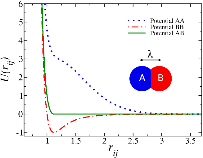
Figure 1: Interaction potentials between particles of type A (potential AA in dotted blue line), between particles of type B (potential BB in dot-dashed red line) and between particles of type A and B (potential AB in solid green line). Potential AB in z-direction gives the interaction between dimers and walls. The inset shows a picture of a Janus dumbbells formed by particles A and B, with monomers separated by a distance $\lambda$.

Particles of type B interact through a standard 12-6 LJ potential, whose equation is the same of first term of Eq. 1. This potential is represented in figure 1 by potential BB. We use a cutoff radius of $r_{c}=2.5$. Finally, the interaction between particles of type A and type B is given by a Weeks-Chandler-Andersen (WCA) potential, defined as Allen and Tildesley (1987)

$$U^{\rm{CSLJ}}(r_{ij})=\left\{\begin{array}[]{ll}U_{{\rm{LJ}}}(r_{ij})-U_{{\rm{LJ}}}(r_{c})\;,\qquad r_{ij}\leq r_{c}\;,\\ 0\;,\qquad\qquad\qquad\qquad\quad r_{ij}>r_{c}\;.\end{array}\right.$$ (2)

The WCA potential considers just the repulsive part of the standard 12-6 LJ potential, as shown in figure 1 by potential AB. Dimers and walls also interact by a WCA potential, but projected in the $z$-direction,

$$U^{\rm{wall}}(z_{ij})=\left\{\begin{array}[]{ll}U_{{\rm{LJ}}}(z_{ij})-U_{{\rm{LJ}}}(z_{c})\;,\qquad z_{ij}\leq z_{c}\;,\\ 0\;,\qquad\qquad\qquad\qquad\quad z_{ij}>z_{c}\;.\end{array}\right.$$ (3)

here, $z_{c}=r_{c}=2^{1/6}\sigma$.

The walls are fixed in $z$-direction separated by a distance of $L_{z}=4\sigma$. We choose this separation to observe the effects of strong confinement, like in quasi-2D thin films. Standard periodic boundary conditions are applied in $x$ and $y$ directions.

The simulations are done in NVT-ensemble using a home made program. The temperature was fixed with the Berendsen thermostat and the equation motions were integrated by velocity Verlet algorithm with a time step $\delta t=0.01$ in reduced unit. The number density is calculated as $\rho=N/V$, where $N$ is the number of monomers particles and $V=L^{2}L_{z}$ is the volume of the simulation box. We simulate systems varying the values of $L$ from $19.0\sigma$ to $60.0\sigma$ to obtain different densities. We use the SHAKE algorithm Ryckaert et al. (1977) to link rigidly each dimer at a distance of $\lambda=0.8\sigma$.

We performed $5\times 10^{5}$ steps to equilibrate the system followed by $5\times 10^{6}$ steps run for the results production stage. The equilibrium state was checked by the analysis of potential and kinetic energies as well the snapshots of distinct simulation times. Simulations with up to $N=5000$ particles were carried out, and essentially the same results were obtained.

The dynamic of the system was analyzed by the lateral mean square displacement and the velocity autocorrelation function $v_{acf}$. The lateral mean square displacement was calculated by

$$\langle[\vec{r}_{\parallel\rm cm}(t)-\vec{r}_{\parallel\rm cm}(t_{0})]^{2}\rangle=\langle\Delta\vec{r}_{\parallel\rm cm}(t)^{2}\rangle\;,$$ (4)

where $\vec{r}_{\parallel\rm cm}(t_{0})=(x_{\rm cm}(t_{0})^{2}+y_{\rm cm}(t_{0})^{2})$ and $\vec{r}_{\parallel\rm cm}(t)=(x_{\rm cm}(t)^{2}+y_{\rm cm}(t)^{2})$ denote the parallel coordinate of the nanoparticle center of mass (cm) at a time $t_{0}$ and at a later time $t$, respectively. Fick diffusion has a diffusion coefficient that can be calculated by Einstein relation,

$$D_{\parallel}=\lim_{t\rightarrow\infty}\frac{\langle\Delta\vec{r}_{\parallel\rm cm}(t)^{2}\rangle}{4t}\;.$$ (5)

The velocity autocorrelation function $v_{acf}$ was evaluated taking the average for all nanoparticles center of mass and initial times

$$v_{acf}=<\vec{v}_{i}(t_{0})\cdot\vec{v}_{i}(t+t_{0})>\;,$$ (6)

where $\vec{v}_{i}(t_{0})$ is the initial velocity for the $i$-th nanoparticle center of mass and $\vec{v}_{i}(t+t_{0})$ is the velocity at an advanced time $t+t_{0}$ for the same particle center of mass.

The system structure was analyzed with the lateral radial distribution function $g_{||}(r_{||})$, evaluated in the $xy$ plane in all phases and defined as Kumar et al. (2005)

$$g_{||}(r)\equiv\frac{1}{\rho^{2}V}\sum_{i\neq j}\delta(r-r_{ij})\left[\theta\left(\left|z_{i}-z_{j}\right|+\frac{\delta z}{2}\right)-\theta\left(\left|z_{i}-z_{j}\right|-\frac{\delta z}{2}\right)\right],$$ (7)

where $\delta(x)$ is the Dirac $\delta$ function and the Heaviside function $\theta(x)$ restricts the sum of particle pair in the same slab of thickness $\delta z=\sigma$.

Directly related to $g_{||}(r_{||})$, we also use the translational order parameter $\tau$, defined as Errington and Debenedetti (2001)

$$\tau\equiv\int^{\xi_{c}}_{0}\mid g_{\parallel}(\xi)-1\mid d\xi,$$ (8)

where $\xi=r_{\parallel}(\rho^{l})^{1/2}$ is the interparticle distance in the direction parallel to the plates scaled by the density of the layer, $\rho^{l}=N^{l}/L^{2}$. $N^{l}$ is the average of particles for each layer. We use $\xi_{c}=(\rho^{l})^{1/2}L/2$ as cutoff distance.

The snapshots of the systems also were used to analyze the self-assembled structures at different densities and temperatures. The pressure-temperature phase diagram was constructed using the parallel pressure ($P_{\parallel}$), calculated by Virial expression in $x$ and $y$ directions. All the system properties were evaluated for all simulated points.

All physical quantities are computed in the standard LJ unitsAllen and Tildesley (1987). Distance, density of particles, time, parallel pressure and temperature are given, respectively, by

$$r^{*}\equiv\frac{r}{\sigma}\;,\quad\rho^{*}\equiv\rho\sigma^{3}\;,\quad\mbox{and}\quad t^{*}\equiv t\left(\frac{\epsilon}{m\sigma^{2}}\right)^{1/2}\;,\quad P_{\parallel}^{*}\equiv\frac{p\sigma^{3}}{\epsilon}\quad\mbox{and}\quad T^{*}\equiv\frac{k_{B}T}{\epsilon}\;,$$ (9)

where $\sigma$, $\epsilon$ and $m$ are the distance, energy and mass parameters, respectively. Considering that, we will omit the symbol ^∗ to simplify the discussion.

III Results and Discussion

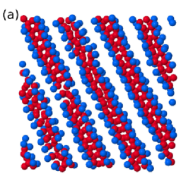
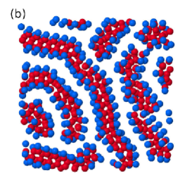
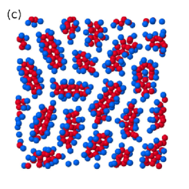
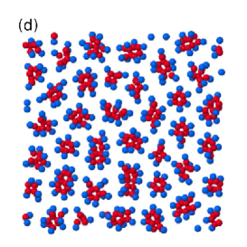
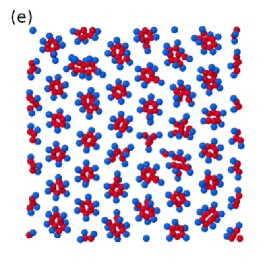
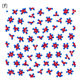
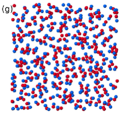
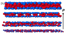
Figure 2: Frontal vision snapshots of confined Janus particles at $\lambda=0.8$. We show (a) Structured elongated micelles (SEM) at $\rho=0.48$ and $T=0.200$, (b) elongated micelles I (EMI) at $\rho=0.50$ and $T=0.100$, (c)elongated micelles II (EMII) at $\rho=0.40$ and $T=0.100$, (d) spherical micelles (SM) at $\rho=0.28$ and and $T=0.100$, (e) hexagonal aggregates (HA) at $\rho=0.25$ and and $T=0.100$, (f) coexistence between hexagonal and trihedral aggregates (TA) at $\rho=0.15$ and and $T=0.100$, (g) fluid phase at $\rho=0.25$ and $T=0.400$. (h) Lateral view of the simulation box showing the bilayer structure for smaller (bottom) and higher (up) densities. For simplicity, the plates are not shown.

Controlling the self-assembly of chemical building blocks in distinct structures is the goal in the studies of confined molecules and nanoparticles with this characteristic Kim and Yi (2015); Rosenthal and Klapp (2005, 2011), as Janus nanoparticles. Therefore, we first report the self-assembled structures observed in our simulations. The aggregates were classified using snapshots, the lateral mean square displacement, the $v_{acf}$ and the $g_{||}(r_{||})$.

The small separation $L_{z}=4.0$ between the plates used in our simulations induces the system to form two layers, one near each plate, regardless the system density, as we shown in figure 2(h). To map the particles arrangement, we analyze the frontal vision of the system, summarized in figure 2. At high temperatures, the system is in a fluid phase, without a defined arrangement. For instance, we can see the snapshot at density $\rho=0.25$ and temperature $T=0.400$, shown in figure 2(g). At lower temperatures, the nanoparticles aggregate. The shape and structure of these aggregates depend on the system density. Let’s take the isotherm $T=0.100$. At the smallest densities, $\rho<0.16$, the system remains in a fluid phase. The aggregation starts at $\rho=0.16$, with the nanoparticles assembled in trihedral (TA3), tetrahedrical (TA4) or hexagonal (HA) aggregates. As the name indicates, the first one is composed of three dimers, the second one by four and the third by six dimers. The snapshot in figure 2(f) shows the coexistence of these aggregates. Increasing the density, the TA3/4 binds and more HA aggregates are observed, as shown in figure 2(e) for $\rho=0.25$.

Spherical micelles (SM) were also obtained, as we show in figure 2(d) for $\rho=0.28$, as well elongated micelles (EMII), shown in figure 2(c). HA, SM and EMII structures were observed in the bulk system Bordin et al. (2015). The confinement leaded to the assembly in TA3/4 at lower densities and longer elongated micelles (EMI) at higher densities. The EMI can show no preferential orientation, as the one shown in figure 2(b) for $\rho=0.50$ and $T=0.100$, or have a well defined orientation, as in the figure 2(a) for $\rho=0.48$ and $T=0.200$. We will refer to this last case of oriented elongated micelles as structured elongated micelles (SEM). The main difference in the aggregation compared to the Brownian system Bordin and Krott (2016) is in the SEM phase. Here, this lamellar phase is straight, while in our previous work we have observed a rippled lammelae structure. Nevertheless, this small structural difference leads to a new dynamical feature, as we discuss below.

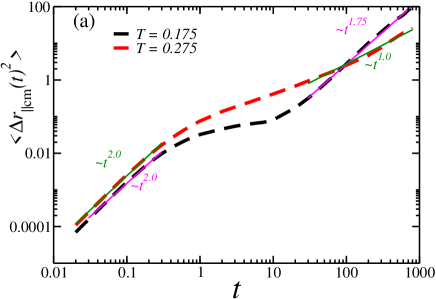
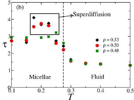
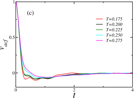
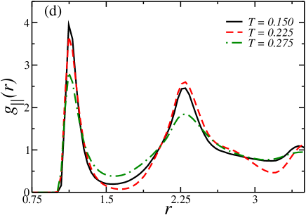
Figure 3: (a) Lateral mean square displacement as function of time for nanoparticles center of mass in the Fick (red dashed line) and superdiffusive (black dashed line) regime. Straight lines in green and magenta are guide to the eyes to show the curves slope. (b) Translational order parameter $\tau$ as function of temperature for distinct isochores showing the relation between the maximum in $\tau$ and the superdiffusivity. (c) Velocity autocorrelation function for $\rho=0.53$ and distinct velocities. (d) Lateral radial distribution function showing the behavior of the first two peaks, related to the two length scales.

The structural and dynamical behavior of two length scale fluids are strongly connected de Oliveira et al. (2006, 2006); Bordin et al. (2013). Therefore, in order to understand the difference between the EMI and SEM aggregates we investigated the dynamical characteristics of these micelles. For instance, we take the isochore $\rho=0.53$, where the Janus dimers are assembled in both EMI and SEM . The lateral mean square displacement for temperature $T=0.275$, red dashed line in figure 3(a), shows an initial ballistic behavior, and a Fick regime as $t\rightarrow\infty$. On the other hand, for $T=0.175$, black dashed curve in figure 3(a), the initial ballistic evolves to a superdiffusive regime, with $\alpha\approx 1.75$. This superdiffusive regime was observed in all SEM structures, with $\alpha$ ranging from $\sim 1.30$ to $\sim 1.80$. For simplicity, we will not show all lateral mean square displacement curves. Basically, in the fluid regions and for all aggregates, except the SEM, the nanoparticles collisions lead the system to the Fick regime. However, in the SEM lamellae phase, the liquid-crystal structure prevents the collisions. As consequence, the dimers moves freely in the line defined by the structure, leading to the superdiffusive regime. For the Brownian system Bordin and Krott (2016), since the lamellae phase is not straight, but rippled, the supperdifusive regime was not observed. This shows how that the white noise and drag force from the Brownian Dynamics effects on the dynamic will reflect in the structure. Particularly, the SEM region corresponds to a region where the translational order parameter $\tau$ has a maximum. This result, shown in figure 3(b), highlights the relation between structure and dynamics. Therefore, the SEM micelles are highly diffused and highly structured aggregates. This relation between structure and dynamics is well known in the literature of anomalous fluids de Oliveira et al. (2006, 2006); Bordin et al. (2013). However, was never relate to anomalous diffusion, only to diffusion anomaly.

The velocity autocorrelation function $v_{acf}$ is a powerful tool to understand the dynamics of the systems. In figure 3(c) we show $v_{acf}$ as function of time for $\rho=0.53$ and temperatures ranging from $T=0.175$ to $T=0.275$. The superdiffusive regime and SEM micelles were observed for $T=0.175$, $0.200$ and $0.225$. As we can see in figure 3(c), at these temperatures the curves cross the zero axis at shorter times than in the Fick regime with EMI micelles, $T=0.250$ and $0.275$. This shows that in the superdiffusive regime the nanoparticles are strongly caged by the neighbors dimers. Thereat, we know that the system has a superdiffusion regime related to a collective behavior and assembly in a specific well structured micelle.

It is well reported in the literature that the competition between the two scales in the Eq. (1) is the main ingredient to a fluid present water-like anomalies de Oliveira et al. (2007). To see the influence of this competition, we analyzed the $g_{||}(r_{||})$ for the A monomers when the system enters and leaves the SEM phase. As we show in figure 3(d), when we walk through the isochore $\rho=0.53$, from $T=0.150$ – before the superdiffusion region – to $T=0.225$ – the limit of the superdiffusion region – the first peak in the $g_{||}(r_{||})$ decays, while the second peak rises. This is the competition between the scales, where the particles moves from one of the preferential distances to the other. As we heat the system, both peaks decays, as when we walk from $T=0.225$ to $T=0.275$ – outside the superdiffusive regime. Therefore, the competition between the two length scales leads the nanoparticles from a non-oriented Fick diffusion elongated micellae phase to a oriented superdiffusive elongated micellae phase.

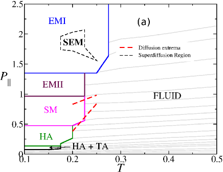
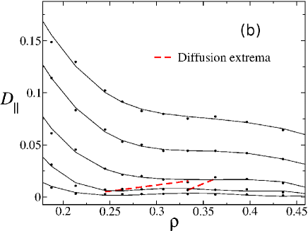
Figure 4: Results for Janus confined particles with $\lambda=0.8$. In (a) we show the parallel pressure versus temperature phase diagram for isochores between $0.05$ and $0.50$ in solid gray lines. In (b) we show the lateral diffusion coefficient as function of time for fixed temperatures of $T=0.150$, $0.200$, $0.250$, $0.300$ and $0.350$.

With this informations, we can draw the $P_{\parallel}-T$ phase diagram for this system, shown in figure 4(a). We should address that the phase diagram is qualitative, based on direct observation of the various assembled structures, the $v_{acf}$, the $g_{||}(r_{||})$ and lateral mean square displacement. The regions where the distinct self-assembled structures were observed are indicated in the phase-diagram. In addition to the anomalous diffusion, the system also shows diffusion anomaly. This anomaly is characterized by the maximum and minimum in the curve of the lateral diffusion coefficient $D_{||}$ as function of density at constant temperature. The figure 4(b) shows these curves, with the diffusion extrema indicated. This extrema is also shown in the phase diagram. Notice that the anomaly region occurs in the fluid and in the SM phase, indicating that the anomaly can be observed in spherical micelles. In this way, it is possible to construct spherical self-assembled structure that will diffuse faster when compressed. As usual, the diffusion anomaly is explained using the competition between the two scales. The graphic showing this was omitted for simplicity, since this result is well known and discussed in the literature de Oliveira et al. (2006); Bordin et al. (2015); Bordin (2016).

Another interesting difference between the Brownian and the molecular system $P_{\parallel}-T$ phase diagram is the absence of a melting induced by the density increase in the SEM phase Bordin and Krott (2016). This suggests that the melting scenario for this Janus nanoparticles is strongly affected by the solvent. As well, the fluid phase structure is also affected. This is evident once for the molecular system we have not observed the density anomaly, only the diffusion anomaly. For the Brownian system, the density anomalous region ended in the melting induced by density increase region. Therefore, this comparison between the Browinian and molecular system has shown that not only the dynamical behavior are distinct, what was expected due the thermostats characteristics, but also the structural, assembly and thermodynamic properties of these nanoparticles are strongly affected.

IV Conclusion

We reported the study of Janus nanoparticles confined in a thin film. Here, the effects of Brownian motion were removed, and we studied the molecular system without solvent. This system has special interest in the design of new material using the confinement to control the self-assembled structures. We have found a rich variety of aggregates and micelles, including structures not observed in the bulk system or in the Brownian system. More than that, our results show that the more structured micelle has an anomalous diffusion, with a superdiffusive regime related to a maximum in the translational order parameter. We have shown that this anomalous diffusion is related to the competition between the two length scales. As well, the system have diffusion anomaly, where the diffusion constant increases with the density increases. These results show that materials which can be modeled by two length scale potentials have an interesting and peculiar behavior. New studies on this system are in progress, as anisotropy effects.

V Acknowledgments

We thank the Brazilian agency CNPq for the financial support.

References

- Roh et al. (2005) K.-H. Roh, D. C. Martin and J. Lahann, Nature Materials, 2005, 4, 759.
- Klapp (2016) S. H. L. Klapp, Curr. Opin. in Coll. and Inter. Sci., 2016, 21, 76–85.
- Liu et al. (2012) Y. Liu, W. Li, T. Perez, J. D. Gunton and G. Brett, Langmuir, 2012, 28, 3–9.
- Whitelam and Bon (2010) S. Whitelam and S. A. F. Bon, J. Chem. Phys., 2010, 132, 074901.
- Munaò et al. (2013) G. Munaò, D. Costa, A. Giacometti, C. Caccamo and F. Sciortino, Phys. Chem. Chem. Phys, 2013, 15, 20590.
- Munaò et al. (2014) G. Munaò, P. O’Toole, T. S. Hudson and F. Sciortino, Soft Matter, 2014, 10, 5269.
- Munaò et al. (2015) G. Munaò, P. O’Toole, T. S. Hudson, D. Costa, C. Caccamo, F. Sciortino and A. Giacometti, J. Phys. Cond. Matt., 2015, 27, 234101.
- Avvisati et al. (2015) G. Avvisati, T. Visers and M. Dijkstra, J. Chem. Phys, 2015, 142, 084905.
- Bordin (2016) J. R. Bordin, Physica A, 2016, 459, 1–8.
- Bordin et al. (2015) J. R. Bordin, L. B. Krott and M. C. Barbosa, Langmuir, 2015, 31, 8577–8582.
- Casagrande et al. (1989) C. Casagrande, P. Fabre, E. Raphaël and M. Veyssié, Europhys. Lett., 1989, 9, 251–255.
- Talapin et al. (2010) D. M. Talapin, J.-S. Lee, M. V. Kovalenko and E. V. Shevchenko, Che. Rev., 2010, 110, 389–458.
- Elsukova et al. (2011) A. Elsukova, Z.-A. Li, C. Möller, M. Spasova, M. Acet, M. Farle, M. Kawasaki, P. Ercius and T. Duden, Phys. Stat. Sol., 2011, 208, 2437–2442.
- Tu et al. (2013) F. Tu, B. J. Park and D. Lee, Langmuir, 2013, 29, 12679–12687.
- Walther and Müller (2008) A. Walther and A. H. E. Müller, Soft Matter, 2008, 4, 663–668.
- Walther and Müller (2013) A. Walther and A. H. E. Müller, Chem. Rev., 2013, 113, 5194–5261.
- Zhang et al. (2015) J. Zhang, E. Luijten and S. Granick, Annu. Rev. Phys. Chem., 2015, 66, 581–600.
- Bickel et al. (2014) T. Bickel, G. Zecua and A. Würger, Phys. Rev. E, 2014, 89, 050303.
- Ao et al. (2015) X. Ao, P. K. Ghosh, Y. Li, G. Schmid, P. Hänggi and F. Marchesoni, Europhys. Lett., 2015, 109, 10003.
- Yin et al. (2001) Y. Yin, Y. Lu and X. Xia, J. Am. Chem. Soc., 2001, 132, 771–772.
- Singh et al. (2014) V. Singh, C. Cassidy, P. Grammatikopoulos, F. Djurabekova, K. Nordlund and M. Sowwan, J. Phys. Chem. C, 2014, 118, 13869–13875.
- Lu et al. (2002) Y. Lu, Y. Yin, Z.-Y. Li and Y. Xia, Nano Lett., 2002, 2, 785–788.
- Yoon et al. (2012) K. Yoon, D. Lee, J. W. Kim and D. A. Weitz, Chem. Commun., 2012, 48, 9056–9058.
- Allen and Tildesley (1987) P. Allen and D. J. Tildesley, Computer Simulation of Liquids, Oxford University Press, Oxford, 1987.
- Banks and Fradin (2005) D. S. Banks and C. Fradin, Biophys. J., 2005, 89, 2960–2971.
- Illien et al. (2014) P. Illien, O. Bénichou, G. Oshanin and R. Voituriez, Phys. Rev. Lett., 2014, 113, 030603.
- ten Hagen et al. (2011) B. ten Hagen, S. van Teeffelen and H. Löwen, J. Phys.: Cond. Matter, 2011, 23, 194119.
- Xue et al. (2016) C. Xue, X. Zheng, K. Chen, Y. Tian and G. Hu, J. Phys. Chem. Lett., 2016, 7, 514–519.
- Netz et al. (2002) P. A. Netz, F. W. Starr, M. C. Barbosa and H. E. Stanley, Physica A, 2002, 314, 470.
- Morishita (2005) T. Morishita, Phys. Rev. E, 2005, 72, 021201.
- Sastry and Angell (2003) S. Sastry and C. A. Angell, Nature Mater., 2003, 2, 739–743.
- Liu et al. (2009) B. Liu, C. Zhang, J. Liu, X. Qu and Z. Yang, Chem Comm, 2009, 26, 3871–3873.
- de Oliveira et al. (2006) A. B. de Oliveira, P. A. Netz, T. Colla and M. C. Barbosa, J. Chem. Phys., 2006, 124, 084505.
- Bordin and Krott (2016) J. R. Bordin and L. B. Krott, Phys. Chem. Chem. Phys., 2016, 18, 28740–28746.
- Munaò and Urbic (2015) G. Munaò and T. Urbic, J. Chem. Phys., 2015, 142, 214508.
- Hus et al. (2015) M. Hus, G. Zakelj and T. Urbic, Acta Chim. Slov., 2015, 62, 524–530.
- Munaò and Saija (2016) G. Munaò and F. Saija, Phys. Chem. Chem. Phys., 2016, 18, 9484–9489.
- Gavazzoni et al. (2014) C. Gavazzoni, G. K. Gonzatti, L. F. Pereira, L. H. C. Ramos, P. A. Netz and M. C. Barbosa, J. Chem. Phys., 2014, 140, 154502.
- de Oliveira et al. (2010) A. B. de Oliveira, E. Nevez, C. Gavazzoni, J. Z. Paukowski, P. A. Netz and M. C. Barbosa, J. Chem. Phys., 2010, 132, 164505.
- de Oliveira et al. (2006) A. B. de Oliveira, P. A. Netz, T. Colla and M. C. Barbosa, J. Chem. Phys., 2006, 125, 124503.
- Kell (1967) G. S. Kell, J. Chem. Eng. Data, 1967, 12, 66.
- Angell et al. (1976) C. A. Angell, E. D. Finch and P. Bach, J. Chem. Phys., 1976, 65, 3063–3066.
- Krott and Barbosa (2013) L. B. Krott and M. C. Barbosa, J. Chem. Phys., 2013, 138, 084505.
- Krott and Barbosa (2014) L. B. Krott and M. C. Barbosa, Phys. Rev. E, 2014, 89, 012110.
- Bordin et al. (2014) J. R. Bordin, L. B. Krott and M. C. Barbosa, J. Chem. Phys., 2014, 141, 144502.
- Krott and Bordin (2013) L. Krott and J. R. Bordin, J. Chem. Phys., 2013, 139, 154502.
- Bordin et al. (2014) J. R. Bordin, L. Krott and M. C. Barbosa, J. Phys. Chem. C, 2014, 118, 9497–9506.
- Krott et al. (2015) L. B. Krott, J. R. Bordin and M. C. Barbosa, J. Phys. Chem. B, 2015, 119, 291–300.
- Bordin et al. (2012) J. R. Bordin, A. B. de Oliveira, A. Diehl and M. C. Barbosa, J. Chem. Phys., 2012, 137, 084504.
- Bordin et al. (2013) J. R. Bordin, A. Diehl and M. C. Barbosa, J. Phys. Chem. B, 2013, 117, 7047–7056.
- Bordin et al. (2014) J. R. Bordin, J. S. Soares, A. Diehl and M. C. Barbosa, J. Chem Phys., 2014, 140, 194504.
- Krott et al. (2015) L. B. Krott, J. R. Bordin, N. Barraz Jr. and M. C. Barbosa, J. Chem. Phys., 2015, 1, 134502.
- Ryckaert et al. (1977) J. P. Ryckaert, G. Ciccotti and H. J. C. Berendsen, J. Comput. Phys., 1977, 23, 327.
- Kumar et al. (2005) P. Kumar, S. V. Buldyrev, F. W. Starr, N. Giovambattista and H. E. Stanley, Phys. Rev. E, 2005, 72, 051503.
- Errington and Debenedetti (2001) J. R. Errington and P. D. Debenedetti, Nature (London), 2001, 409, 318.
- Kim and Yi (2015) M. P. Kim and G.-R. Yi, Frontiers in Materials, 2015, 2, 45.
- Rosenthal and Klapp (2005) G. Rosenthal and S. H. L. Klapp, Int. J. Mol. Sci., 2005, 13, 9431.
- Rosenthal and Klapp (2011) G. Rosenthal and S. H. L. Klapp, J. Chem. Phys., 2011, 134, 154707.
- de Oliveira et al. (2007) A. B. de Oliveira, P. A. Netz and M. C. Barbosa, Physica A, 2007, 386, 744–747.