Regime shifts driven by dynamic correlations in gene expression noise

Abstract

Gene expression is a noisy process that leads to regime shift between alternative steady states among individual living cells, inducing phenotypic variability. The effects of white noise on the regime shift in bistable systems have been well characterized, however little is known about such effects of colored noise (noise with non-zero correlation time). Here, we show that noise correlation time, by considering a genetic circuit of autoactivation, can have significant effect on the regime shift in gene expression. We demonstrate this theoretically, using stochastic potential, stationary probability density function and first-passage time based on the Fokker-Planck description, where the Ornstein-Uhlenbeck process is used to model colored noise. We find that increase in noise correlation time in degradation rate can induce a regime shift from low to high protein concentration state and enhance the bistable regime, while increase in noise correlation time in basal rate retain the bimodal distribution. We then show how cross-correlated colored noises in basal and degradation rates can induce regime shifts from low to high protein concentration state, but reduce the bistable regime. In addition, we show that early warning indicators can also be used to predict shifts between distinct phenotypic states in gene expression. Predictions that a cell is about to shift to a harmful phenotype could improve early therapeutic intervention in complex human diseases.

I Introduction

Natural systems can undergo sudden, large and irreversible changes under the influence of small stochastic perturbations Book_Sch ; ScJo09 . Such qualitative sudden changes are known as “regime shifts” have been found in a variety of ecological systems Sc01 ; ScCa2003 ; Wang:2012 , climate systems LeHeKr08 , biological systems Ve05 ; Mc03 ; kor2014 ; Ri2016 , financial markets MaLeSu08 , physical systems FoWh15 ; GoSh:2016 , etc. It has been identified that regime shifts generally occur at tipping points (namely bifurcation points) ScJo09 ; Scheffer:2012sc , where the system abruptly shifts from one stable state to another stable state. There are also examples of purely noise induced regime shifts (known as stochastic switching) DaCa15 ; SKP14 ; Sh2016 . Regime shifts have the potential to invoke serious and harmful consequences for environment as well as human well-being Sc01 ; FoWh15 ; Ri2016 .

Understanding the mechanisms of regime shifts and predicting them using early warning signals (EWS) have been recently emerged as a challenging area of research due to the potential application in management and prevention of sudden catastrophes in complex systems. Numerous studies have been carried out to develop EWS for successfully predicting regime shifts Dakos:2012pone ; Scheffer:2012sc ; CaBr08 ; GuJa08 ; ScJo09 . Extensive research on EWS suggests that statistical signatures, such as concurrent increase in “variance”, “autocorrelation”, “skewness” can predict regime shifts in a wide variety of complex systems ScJo09 ; Scheffer:2012sc ; GuJa08 . These EWS are mainly derived from the phenomenon of critical slowing down, which is associated with a tipping point at which the stability of an equilibrium state changes as the dominant real eigenvalue becomes zero Book_Sch ; ScJo09 ; Scheffer:2012sc . As a result, rate of recovery from small stochastic perturbations becomes slow as the system approaches a tipping point, resulting concurrent increase in variance, autocorrelation and skewness prior to a regime shift. However, sometimes these EWS are not present before a regime shift due to statistical limitations and confer false alarms sc2015 . In such a situation, apart from the aforementioned indicators, other indicators, e.g., “conditional heteroskedasticity” Se11 ; En1982 can be very useful to detect regime shifts. Conditional heteroskedasticity is used to investigate the possible links between time series data and their volatilities En1982 . This indicator generally avoids the chance of false alarms as it is associated with significant test and their probabilities. Majority of the earlier studies on predicting regime shifts using EWS have focused on the ecological and climate systems Book_Sch ; DaCa15 ; sc2015 . However, few recent studies have reported the huge potential of EWS as risk markers from molecular biology to chronic human diseases PaPaBo13 ; kor2014 ; gl15 ; TrAn15 ; Sh2016 ; Ri2016 .

Regime shifts those arise in medical conditions can increase the risk of diseases and even result in sudden death gl15 ; Ri2016 . Recently, EWS for detecting regime shifts in ecology have got special attention in medical sciences ChLi12 ; kor2014 ; Ri2016 . The ability to predict such regime shifts could prove fruitful in early detection of diseases Van2014 ; La2012 ; kra2012 ; Sc2013 . An important example of regime shift in molecular biology is genetic regulatory system, which includes sudden transition in protein production level in individual cells resulting disease onset Sm98 . In genetically identical cells fluctuations in transcription and translation give rise to regime shifts between alternative states (i.e., phenotypic variability) in intracellular protein concentrations KaEl05 . Indeed, in positive-feedback regulation individual cells can exist in different steady states, some live in the “on” expression state and others live in the “off” expression state Ha00 . These “on” and “off” states are mainly related with protein production. Also, the cells perform a range of specialized functions for protein production that depend upon gene expression states. For instance, $\beta$ cells in the pancreas produce the protein hormone insulin that depends upon HLA-encoding gene states, $\alpha$ cells produce the hormone glucagon, lymphocytes of the immune system produce antibodies-proteins (gamma globulin’s), while developing red blood cells produce the oxygen-transport protein hemoglobin. Finding the causes of regime shift and predicting that a cell is about to shift to a harmful gene expression state can improve critical care management for complex human diseases.

In previous studies, the stochastic fluctuations associated with gene expression are considered as Gaussian white noise (noise with zero correlation time) Ha00 ; LiJi04 ; Ch08 ; Frcasaib12 ; Gh12 . In contrast, few recent studies have shown that gene expression noise can also be colored in nature (noise with non-zero correlation time) Ro2005 ; Si2006 ; ShOSw08 ; du2008 ; Dunlop:thesis2008 . These studies have measured the variability of protein levels in human cellular system and showed that cell to cell variability of protein levels can be correlated over generations Si2006 . It has also been measured experimentally that gene expression noise has a finite correlation time ShOSw08 . Moreover, colored noise can break bistability in different ways than that of white noise Kl1988 . In order to address these issues, it is important to study the effects of noise correlation on regime shifts in gene expression.

One of the key questions addressed in this paper is: How the dynamic correlation in gene expression noise affects the characteristics of sudden regime shifts between alternative steady states (i.e., low and high protein concentration states)? For this, we begin with a stochastic version of gene regulatory system: a genetic autoactivating switch. The colored noise is modeled using Ornstein-Uhlenbeck process. We compute the stochastic potential and the stationary probability density function to quantify the effects of noise intensity and correlation time on the relative stability of alternative steady states using Fokker-Planck description. We then obtain the mean first-passage time (MFPT) for escape over the potential barrier. We show that increase in the noise correlation time in degradation rate can induce a regime shift from low to high protein concentration state and enhance the bistable regime, while noise in basal rate retain the bimodal distribution of the system steady states. We also show that cross-correlated colored noises in basal and degradation rates can induce regime shifts from low to high protein concentration state, however reduce the bistable regime. Further, we examine EWS prior to a regime shift in gene expression dynamics, which can prove to be very useful to predict that a cell is about to shift to a harmful phenotype.

The paper is organized as follows: Section II presents the description of a stochastic model of gene expression. In Sec. III.1, steady state analysis of the stochastic model is presented. Impacts of noise correlation time, noise intensity and cross-correlation strength on the effective potential landscape and the stationary probability density function are calculated in Sec. III.2. We then examine the MFPT of the system driven by the correlated noise in Sec. III.3, and precursors of regime shift in Sec. III.4. Finally, in Sec. IV, we conclude the study by discussing the key findings reported in this paper.

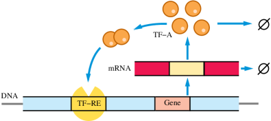
Figure 1: (Color online) A schematic of the autoactivating genetic switch. The expression of gene leads to protein monomers (TF-A) and after oligomerization they bind to the upstream regulatory site (TF-RE), activating production of monomers. Degradation of protein and mRNA are denoted by the slashed circles ($\varnothing$).

II A stochastic model of gene expression

To understand the effects of noise correlation, we consider a well studied stochastic model of gene expression: the autoactivating switch, which consists multiple stable states BeSeSe01 ; TyChNo03 ; Ch08 ; Frcasaib12 . A schematic picture of the genetic circuit is shown in Fig. 1, which involves a single gene that transcribes a single protein called activator TF-A. On dimerization the protein TF-A dimer stimulates transcription when binds to the responsive element TF-RE in the DNA sequence. The mRNA produced in transcription and protein monomer produced in translation then follow post-transcriptional degradation which is an important regulatory step (see Fig. 1) Is2003 . Letting $x(t)$ and $y(t)$ as concentrations of the activator protein TF-A and the mRNA respectively, we can write the rate equations describing the evolution of $x(t)$ and $y(t)$:

$$\frac{dx}{dt} =Ky-k_{deg_{r}}x,$$ (1a)

$$\frac{dy}{dt} =F(x)-k_{deg_{m}}y,$$ (1b)

where the parameter $K$ is the translation rate, $F(x)$ is the mRNA transcription rate, $k_{deg_{r}}$ and $k_{deg_{m}}$ are the degradation rates of the protein monomers and the mRNA. The function $F(x)$ is given by a Hill-type function Tha2001 :

$$F(x)=\frac{k_{max}\>x^{\mathcal{H}}}{k_{d}+x^{\mathcal{H}}}+k_{f},$$

where $k_{max}$ is the maximum transcription rate, $k_{d}$ is the Hill constant, $k_{f}$ is the basal transcription rate and $\mathcal{H}$ is the Hill coefficient which we consider $\mathcal{H}=2$ ZhYaTa11 . The degradation rate of mRNA molecules is usually much faster than that of proteins Tha2001 , i.e., $k_{deg_{m}}>>k_{deg_{r}}$.

Since the fast reactions equilibrate quickly, to reduce the dimension of the system it is useful to apply the quasi-steady state approximation (QSSA) which replaces state variables involved in the fast reactions with their equilibrium values. This dimension reduction greatly simplifies the complexity of the system Ra03 . Now employing the QSSA in Eq. (1) by replacing the equilibrium value $y=F(x)/k_{deg_{m}}$ from the “fast” Eq. (1b) into the “slow” Eq. (1a) and taking $\mathcal{H}=2$, we obtain the following reduced system:

$$\frac{dx}{dt}=\frac{K}{k_{deg_{m}}}\left(\frac{k_{max}x^{2}}{k_{d}+x^{2}}+k_{f}\right)-k_{deg_{r}}x\>.$$ (2)

The above Eq. (2) can also be written as WeBu13 :

$$\frac{dx}{dt}=R+a\frac{x^{2}}{k_{d}+x^{2}}-k_{deg_{r}}x,$$ (3)

where $R=\frac{k_{f}K}{k_{deg_{m}}}$ is the basal expression rate and $a=\frac{k_{max}K}{k_{deg_{m}}}$ is the maximum transcription rate. Now the dimensionless version of equation Eq. (3) is:

$$\frac{d\tilde{x}}{d\tilde{t}}=\tilde{r}+\tilde{a}\frac{\tilde{x}^{2}}{1+\tilde{x}^{2}}-\tilde{x},$$ (4)

where $\tilde{x}=\frac{x}{\sqrt{k_{d}}}$, $\tilde{t}=k_{deg_{r}}t$, $\tilde{a}=\frac{a}{k_{deg_{r}}\sqrt{k_{d}}}$, and $\tilde{r}=\frac{R}{k_{deg_{r}}\sqrt{k_{d}}}$. Finally, we use $x$, $t$, $r$ and $a$ in place of $\tilde{x}$, $\tilde{t}$, $\tilde{r}$ and $\tilde{a}$, and Eq. (4) reads:

$$\frac{dx}{dt}=r+a\frac{x^{2}}{1+x^{2}}-x\;.$$ (5)

For a range of $a$, if $0<r<1/3\sqrt{3}\approx 0.19245\>$ then Eq. (5) exhibits two types of asymptotic behaviors: monostability and bistability (i.e., it leads to phenotypic variability) WeBu13 . In the case of bistability the system has three equilibrium points, the middle one (say $x_{u}$) is unstable and the other two are stable. In the bistable regime, the initial condition (say $x_{i}$) plays a key role in determining the final equilibrium state of the system. All the initial values $x_{i}>x_{u}$ will evolve to the upper equilibrium point and others $x_{i}<x_{u}$ will evolve to the lower equilibrium point in the stationary state. Figure 2 depicts the phase diagram of the model (5) in the $(a,r)$-plane for different values of the control parameters $a$ and $r$. The region of bistability is bounded by a saddle-node bifurcation curve at which transition occurs from monostable to bistable regime or vice versa. A thorough analysis of the deterministic model (5) is given in Sm98 .

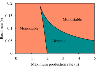
Figure 2: (Color online) Phase diagram of the gene expression model (5) in $(a,r)-$plane. The curve separating the monostable region from the bistable region is a saddle-node bifurcation curve.

As already discussed in the introduction, here we are mainly interested in understanding the effects of correlated gene expression noise on the regime switching between two alternative steady states. Therefore, in the model (5) we incorporate correlated stochastic process in the form of two fluctuating rates. We assume that variability in the basal and the degradation rates causes the production rate of protein to fluctuate LiJi04 . That is, in Eq. (5) the basal rate varies stochastically as $r\rightarrow r+\eta(t)$ and also the degradation rate varies stochastically as $1\rightarrow 1+\xi(t)$. We consider $\xi(t)$ and $\eta(t)$ to be Ornstein-Uhlenbeck (OU) processes Ga85 : positively correlated Gaussian noise (i.e., colored Gaussian noise) with a zero mean and correlation time $\tau_{1}$ and $\tau_{2}$, respectively. The Langevin equation corresponding to Eq. (5) which contains both the Gaussian colored noises $\eta(t)$ and $\xi(t)$ can be written as Ha00 ; LiJi04 :

$$\frac{dx}{dt} = (r+\eta(t))+a\frac{x^{2}}{1+x^{2}}-(1+\xi(t))x,$$ (6)

$$= f(x)+g_{1}(x)\xi(t)+g_{2}(x)\eta(t),$$

where $f(x)=r+\frac{ax^{2}}{1+x^{2}}-x$, $g_{1}(x)=-x$ and $g_{2}(x)=1$. Thus, here the noise $\xi(t)$ can be considered as multiplicative colored noise in comparison to $\eta(t)$, which works as additive colored noise Ha00 . The OU processes $\xi(t)$ and $\eta(t)$ satisfy the following equations:

$$\dot{\xi}(t) = -\frac{\xi(t)}{\tau_{1}}+\frac{\sqrt{2\sigma_{1}}}{\tau_{1}}\xi_{1}(t),$$

$$\dot{\eta}(t) = -\frac{\eta(t)}{\tau_{2}}+\frac{\sqrt{2\sigma_{2}}}{\tau_{2}}\eta_{1}(t),$$

where $\xi_{1}(t)$ and $\eta_{1}(t)$ are white Gaussian noises with zero mean and unit variance Ga85 . The parameters $\sigma_{i}$ and $\tau_{i}(\neq 0)$, for $i=1,2$ are noise strength and self correlation time of $\xi(t)$ and $\eta(t)$, respectively. The colored Gaussian noises $\xi(t)$ and $\eta(t)$ satisfy the following statistical properties:

$$\langle\xi(t)\rangle=\langle\eta(t)\rangle=0,$$

$$\langle\xi(t)\xi(t^{\prime})\rangle=(\sigma_{1}/\tau_{1})\exp(-|t-t^{\prime}|/\tau_{1}),$$

$$\langle\eta(t)\eta(t^{\prime})\rangle=(\sigma_{2}/\tau_{2})\exp(-|t-t^{\prime}|/\tau_{2}),$$

$$\langle\xi(t)\eta(t^{\prime})\rangle=(\lambda\sqrt{\sigma_{1}\sigma_{2}}/\tau_{3})\exp(-|t-t^{\prime}|/\tau_{3}),$$

where $\lambda$ measures the coupling strength between $\xi(t)$ and $\eta(t)$, $\tau_{3}$ is the correlation time between the noises, while $t$ and $t^{\prime}$ denote two different moments.

In order to understand the influence of colored noises on the rapid switching between two alternative stable states, we employ theoretical calculations of probability densities, potential functions, and MFPTs of Eq. (6).

III Results

III.1 Steady state analysis of the stochastic system

To solve the stochastic Eq. (6), we begin with the probability density $P(x,t)$, which is the probability that the protein concentration will attain the value $x$ at time $t$. The approximate Fokker-Planck equation (AFPE) for $P(x,t)$ corresponding to Eq. (6) is Sa1982 ; liang2004 :

$$\frac{\partial P(x,t)}{\partial t}=-\frac{\partial}{\partial x}\left[A(x)P(x,t)\right]+\frac{\partial^{2}}{\partial^{2}x}[B(x)P(x,t)],$$ (8)

where,

$$A(x) =f(x)+\frac{\sigma_{1}x}{1-\tau_{1}f^{\prime}(x_{s})}-\frac{\lambda\sqrt{\sigma_{1}\sigma_{2}}}{1-\tau_{3}f^{\prime}(x_{s})},$$ (9a)

$$B(x) =\frac{\sigma_{1}x^{2}}{1-\tau_{1}f^{\prime}(x_{s})}-\frac{2\lambda\sqrt{\sigma_{1}\sigma_{2}}x}{1-\tau_{3}f^{\prime}(x_{s})}+\frac{\sigma_{2}}{1-\tau_{2}f^{\prime}(x_{s})},$$ (9b)

and $f^{\prime}(x_{s})$ is the derivative of $f(x)$ at the equilibrium point $x_{s}$. The derivative $f^{\prime}(x_{s})$ is given by:

$$f^{\prime}(x_{s})=\frac{2ax_{s}}{(1+x_{s}^{2})^{2}}-1,$$

where the equilibrium point $x_{s}$ is:

$$x_{s} = \sqrt[3]{-\frac{m}{2}+\sqrt{\Big{(}\frac{m}{2}\Big{)}^{2}+\Big{(}\frac{l}{3}\Big{)}^{3}}}$$ (10)

$$+\sqrt[3]{-\frac{m}{2}-\sqrt{\Big{(}\frac{m}{2}\Big{)}^{2}+\Big{(}\frac{l}{3}\Big{)}^{3}}}-\frac{n}{3},$$

with $l$, $m$ and $n$ are as: $l=1-\frac{(r+a)^{2}}{3}$, $m=\frac{1}{27}(r+a)^{3}+\frac{l}{3}(r+a)-r$, and $n=-(r+a)$. The point $x_{s}$ is the only real solution of $f(x)=0$. Relation between the two functions $A(x)$ and $B(x)$ are given by:

$$A(x)=f(x)+\frac{1}{2}\frac{d}{dx}B(x).$$

Moreover, the AFPE (8) is valid for $1-\tau_{i}f^{\prime}(x_{s})>0$ ($i=1,2,3$) liang2004 .

The stationary probability density function (SPDF) $P_{s}(x)$ of $x$, which is the stationary solution of the AFPE (8), is given by:

$$P_{s}(x) = \frac{N_{c}}{B(x)}\exp\Big{[}\int^{x}\frac{A(u)}{B(u)}du\Big{]}$$

$$= \frac{N_{c}}{\frac{\sigma_{1}x^{2}}{1-\tau_{1}f^{\prime}(x_{s})}-\frac{2\lambda\sqrt{\sigma_{1}\sigma_{2}}x}{1-\tau_{3}f^{\prime}(x_{s})}+\frac{\sigma_{2}}{1-\tau_{2}f^{\prime}(x_{s})}}\times$$

$$\!\!\!\!\!\!\!\!\!\exp\left[\int^{x}\frac{f(u)+\frac{\sigma_{1}u}{1-\tau_{1}f^{\prime}(x_{s})}-\frac{\lambda\sqrt{\sigma_{1}\sigma_{2}}}{1-\tau_{3}f^{\prime}(x_{s})}}{\frac{\sigma_{1}u^{2}}{1-\tau_{1}f^{\prime}(x_{s})}-\frac{2\lambda\sqrt{\sigma_{1}\sigma_{2}}u}{1-\tau_{3}f^{\prime}(x_{s})}+\frac{\sigma_{2}}{1-\tau_{2}f^{\prime}(x_{s})}}du\right],$$

where $N_{c}$ is normalization constant obtained from:

$$\int_{0}^{\infty}P_{s}(x)dx=1.$$

In analogy with the physical situation of a particle moving in a potential, the SPDF peaks correspond to the valleys of the potential (i.e., attractors) and troughs correspond to the tops of the potential (i.e., repellors). We can also introduce a stochastic potential by writing the SPDF (LABEL:Eq:Spdf2) in the form:

$$P_{s}(x)=N_{c}e^{-\phi(x)},$$ (12)

where

$$\phi(x) =\frac{1}{2}\ln\left[\frac{\sigma_{1}x^{2}}{1-\tau_{1}f^{\prime}(x_{s})}-\frac{2\lambda\sqrt{\sigma_{1}\sigma_{2}}x}{1-\tau_{3}f^{\prime}(x_{s})}+\frac{\sigma_{2}}{1-\tau_{2}f^{\prime}(x_{s})}\right]$$ (13)

$$-\int^{x}\frac{f(u)}{\frac{\sigma_{1}u^{2}}{1-\tau_{1}f^{\prime}(x_{s})}-\frac{2\lambda\sqrt{\sigma_{1}\sigma_{2}}u}{1-\tau_{3}f^{\prime}(x_{s})}+\frac{\sigma_{2}}{1-\tau_{2}f^{\prime}(x_{s})}}du,$$

is the stochastic potential of the system. The stochastic potential provides information about the the relative stability of the steady states, likewise the deterministic potential of a system.

It is also important to know the stationary state of the system for arbitrary noise intensities. More specifically, we are interested in understanding the transition phenomena between stationary states that occur due to the presence of correlated noise. For the deterministic model (5), this can be best visualized by the corresponding bifurcation diagram representing the equilibrium protein concentration $x$, for a range of control parameter. In the stochastic model (6), a qualitative change in the stationary state is accurately reflected by the behavior of the extrema of the SPDF $P_{s}(x)$ WhoRle84 . The extrema of $P_{s}(x)$ can easily be found form the equation given below WhoRle84 :

$$f(x)-\frac{\sigma_{1}x}{1-\tau_{1}f^{{}^{\prime}}(x_{s})}+\frac{\lambda\sqrt{\sigma_{1}\sigma_{2}}}{1-\tau_{3}f^{{}^{\prime}}(x_{s})}=0.$$ (14)

Using the above steady state calculations of the stochastic model (6), in next subsection we mainly focus on the dynamical consequences due to the presence of dynamic correlations in noise.

III.2 Effective potential landscape and stationary probability density function

In order to study the effects of variations in the stochastic parameters (i.e., $\sigma_{i}$, $\tau_{i}$ and $\lambda$), we use the evolution equation for SPDF (LABEL:Eq:Spdf2). The SPDF, potential function and extrema of SPDF are examined for three different cases: (i) When noise is present only in the degradation rate. (ii) When noise is present only in the basal rate. (iii) When noise is present in both the rates, respectively. In Table I, we summarize the values of stochastic parameters corresponding to the above three cases.

Table 1: Stochastic parameter values corresponding to three different cases: Colored noise in (i) the degradation rate, (ii) the basal rate and (iii) noise in both the degradation and basal rates.

Parameters:     $\sigma_{1}$       $\sigma_{2}$       $\lambda$       $\tau_{1}$       $\tau_{2}$       $\tau_{3}$
Case (i):	$\neq 0$	$=0$	$=0$	$\neq 0$	$=0$	$=0$
Case (ii):	$=0$	$\neq 0$	$=0$	$=0$	$\neq 0$	$=0$
Case (iii):	$\neq 0$	$\neq 0$	$\neq 0$	$\neq 0$	$\neq 0$	$\neq 0$

III.2.1 Correlated noise in the degradation rate

We now consider the presence of correlated Gaussian noise which alters the degradation rate in Eq. (6). The corresponding Langevin Eq. (6) can be rewritten in the form:

$$\frac{dx}{dt}=r+a\frac{x^{2}}{1+x^{2}}-(1+\xi(t))x.$$ (15)

Here the noise $\xi(t)$ is modulated due to the multiplication with the state variable $x$. Therefore, a small random fluctuation in the degradation rate can lead to a sudden regime shift in the protein concentration. The role of noise intensity $\sigma_{1}$ and correlation time $\tau_{1}$ of the noise $\xi(t)$ are very important factors, because they can act as system parameters. For fixed values of the control parameters $r$ and $a$, changes in the noise intensity $\sigma_{1}$ and the correlation time $\tau_{1}$ can trigger sudden regime shifts in the level of protein concentration.

From Eq. (LABEL:Eq:Spdf2), the SPDF corresponding to Eq. (15) can be rewritten as:

$$P_{s}(x) = \frac{N_{c}}{B(x)}\exp\Big{[}\int^{x}\frac{A(u)}{B(u)}du\Big{]}$$

$$= \frac{N_{c}}{\frac{\sigma_{1}x^{2}}{1-\tau_{1}f^{\prime}(x_{s})}}\times\exp\left[\int^{x}\frac{f(u)+\frac{\sigma_{1}u}{1-\tau_{1}f^{\prime}(x_{s})}}{\frac{\sigma_{1}u^{2}}{1-\tau_{1}f^{\prime}(x_{s})}}du\right].$$

The potential function is derived from Eq. (13) and is given by:

$$\phi(x)=\frac{1}{2}\ln\left[\frac{\sigma_{1}x^{2}}{1-\tau_{1}f^{{}^{\prime}}(x_{s})}\right]-\int^{x}\frac{f(u)}{\frac{\sigma_{1}u^{2}}{1-\tau_{1}f^{\prime}(x_{s})}}du.$$ (17)

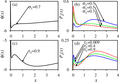
Figure 3: (Color online) Stochastic potential $\phi(x)$ and SPDF $P_{s}(x)$ of the system (15): (a) $\phi(x)$ for the noise intensity $\sigma_{1}=0.7$, and (b) $P_{s}(x)$ for three different values of noise intensity $\sigma_{1}=0.3$ (blue curve), $\sigma_{1}=0.5$ (green curve) and $\sigma_{1}=0.7$ (red curve) with fixed $\tau_{1}=0.5$, $r=0.1$ and $a=3\>$. (c) $\phi(x)$ for the correlation time $\tau_{1}=0.9$, and (d) $P_{s}(x)$ for three different correlation time $\tau_{1}=0.009$ (blue curve), $\tau_{1}=0.4$ (green curve) and $\tau_{1}=0.9$ (red curve) with fixed $\sigma_{1}=0.5$, $r=0.1$ and $a=3.5\>$. The increase in $\sigma_{1}$ induces regime shift from high to low protein concentration state, whereas increase in correlation time $\tau_{1}$ induces regime shift from low to high protein concentration state.

The role of correlated noise on the relative stability between two alternative steady states can be well understood by illustrating the SPDF (LABEL:Eq:Spdf1) and the potential (17) for an exemplary set of parameters. Figures 3(a)-(b) show the influence of the colored noise intensity $\sigma_{1}$ on the shape of the potential $\phi(x)$ and the SPDF $P_{s}(x)$. It can be seen that for a fixed value of $\tau_{1}$, increasing values of $\sigma_{1}$ entail an increase in the likelihood of undesired regime shifts from one stable state to another stable state (Fig. 3(a)). With increasing values of $\sigma_{1}$, the SPDF peak at the low protein concentration $x$ is increasing and that of the high protein concentration $x$ is decreasing. Hence, an increase in the noise intensity $\sigma_{1}$ can induce a sudden regime shift from high to low protein concentration state. However, the dynamic correlation time $\tau_{1}$ has inverted effect on the steady states of the system (Figs. 3(c)–(d)). Figure 3(d) depicts the changes in the SPDF $P_{s}(x)$ peaks with changes in $\tau_{1}$ for a fixed value of $\sigma_{1}$. It is evident from the $P_{s}(x)$ peaks that at low values of $\tau_{1}$ the lower state is more stable and at high values of $\tau_{1}$ the upper state becomes more stable. In fact, $\tau_{1}$ has nontrivial effect on the stationary state and an increase in $\tau_{1}$ can cause a regime shift form low to high protein concentration state. The above results indicate that probability of shifting to the lower stable state is more in the case of increasing noise intensity $\sigma_{1}$, whereas probability of finding upper stable state is more in the case of increasing correlation time $\tau_{1}$. Figure 4 shows the continuous evolution of the SPDF $P_{s}(x)$ with increasing values $\tau_{1}$.

Figure 4: (Color online) The evolution of SPDF $P_{s}(x)$ of the system (15) for continuously changing the correlation time $\tau_{1}$. The other parameters are $\sigma_{1}=0.5$, $r=0.1$ and $a=3.5$. As the $P_{s}(x)$ corresponding the right potential well has increased with increase in the $\tau_{1}$, the system experiences a regime shift from low to high protein concentration state.

From Eq. (14), now the extrema of $P_{s}(x)$ can be written as:

$$f(x)-\frac{\sigma_{1}x}{1-\tau_{1}f^{\prime}(x_{s})}=0.$$ (18)

Using the above Eq. (18), the extrema of $P_{s}(x)$ is plotted in Fig. 5 as a function of the maximum transcription rate $a$. With the help of the extrema, we investigate the occurrence of critical transition (i.e., any qualitative changes in the stationary state) in the stochastic system (6) by changing the noise intensity $\sigma_{1}$ and the correlation time $\tau_{1}$. Changes in $\sigma_{1}$ and $\tau_{1}$ have opposite effects on the steady state behavior of the system. For a fixed $\tau_{1}$, increasing values of $\sigma_{1}$ decreases the bistability regime (Fig. 5(a)) and for a fixed $\sigma_{1}$, increasing values $\tau_{1}$ increases the bistability regime (Fig. 5(b)).

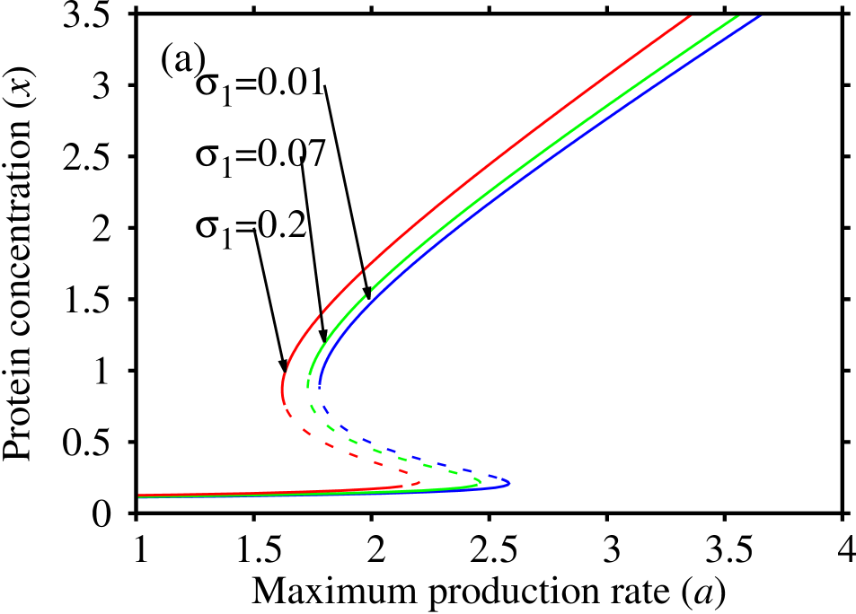
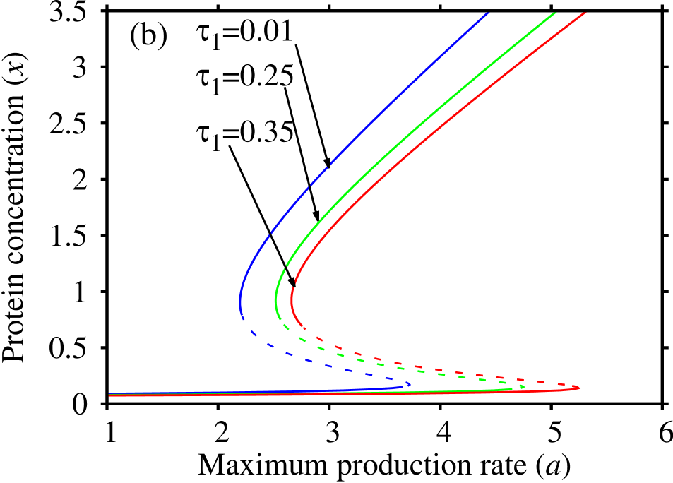
Figure 5: (Color online) Extrema of the SPDF $P_{s}(x)$ of the gene regulation model (15) coupled with noise only in the degradation rate, as a function of $a$: (a) For a fixed $\tau_{1}=1.9$ and increasing values of $\sigma_{1}$, and (b) for a fixed $\sigma_{1}=0.2$ and increasing values $\tau_{1}$. The other parameters are $r=0.1$, $\sigma_{2}=0$, $\tau_{2}=0$, $\tau_{3}=0$ and $\lambda=0$. The increase in $\sigma_{1}$ reduces the bistability regime, whereas increase in $\tau_{1}$ increases the bistabiltiy regime.

III.2.2 Correlated noise in the basal rate

We now focus only on the effect of correlated noise source $\eta(t)$ in the basal rate in Eq. (6) with stochastic parameters $\sigma_{2}\neq 0$ and $\tau_{2}\neq 0$ (see Table I). In this case, Eq. (LABEL:Eq:Spdf2) can be written as:

$$P_{s}(x) = \frac{N_{c}}{B(x)}exp\Big{[}\int^{x}\frac{A(u)}{B(u)}du\Big{]}$$

$$= \frac{N_{c}}{\frac{\sigma_{2}}{1-\tau_{2}f^{\prime}(x_{s})}}\exp\left[\int^{x}\frac{f(u)}{\frac{\sigma_{2}}{1-\tau_{2}f^{\prime}(x_{s})}}du\right],$$

and the potential function is derived from Eq. (13) is given by:

$$\phi(x)=\frac{1}{2}\ln\left[\frac{\sigma_{2}}{1-\tau_{2}f^{\prime}(x_{s})}\right]-\int^{x}\frac{f(u)du}{\frac{\sigma_{2}}{1-\tau_{2}f^{\prime}(x_{s})}}.$$ (20)

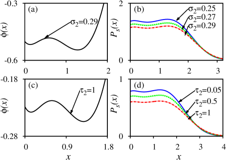
Figure 6: (Color online) Stochastic potential $\phi(x)$ and SPDF $P_{s}(x)$ when noise is present only in the basal rate: (a) $\phi(x)$ for the noise intensity $\sigma_{2}=0.29$, and (b) $P_{s}(x)$ for three different values of the noise intensity $\sigma_{2}=0.25$ (blue curve), $\sigma_{2}=0.27$ (green curve) and $\sigma_{2}=0.29$ (red curve) with fixed $\tau_{2}=1$, $r=0.1$ and $a=1.9$. (c) $\phi(x)$ for the correlation time $\tau_{2}=1$, and (d) $P_{s}(x)$ for three different of the correlation time $\tau_{2}=0.05$ (blue curve), $\tau_{2}=0.5$ (green curve) and $\tau_{2}=1$ (red curve) with fixed $\sigma_{2}=0.5$, $r=0.1$ and $a=1.9$. The increase in $\sigma_{2}$ and $\tau_{2}$ has not much effect on $\phi(x)$ and $P_{s}(x)$, however, both the valleys and tops of $P_{s}(x)$ decay in height.

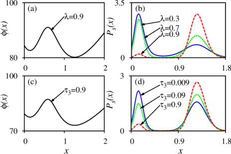
Figure 7: (Color online) Stochastic potential $\phi(x)$ and SPDF $P_{s}(x)$, when the model (6) driven by cross-correlated noises: (a) $\phi(x)$ for the cross-correlation strength $\lambda=0.9$, and (b) $P_{s}(x)$ for three different values of the cross-correlation strength $\lambda=0.3$ (blue curve), $\lambda=0.7$ (green curve) and $\lambda=0.9$ (red curve) with $a=1.9$, $r=0.1$, $\sigma_{1}=0.01$, $\sigma_{2}=0.004$, $\tau_{1}=0.01$, $\tau_{2}=0.08$ and $\tau_{3}=0.03$. (c) $\phi(x)$ for the correlation time $\tau_{3}=0.9$, and (d) $P_{s}(x)$ for three different values of the correlation time $\tau_{3}=0.009$ (blue curve), $\tau_{3}=0.09$ (green curve) and $\tau_{3}=0.9$ (red curve) with $a=1.9$, $r=0.1$, $\sigma_{1}=0.01$, $\sigma_{2}=0.004$, $\lambda=0.3$, $\tau_{1}=0.01$ and $\tau_{2}=0.08$. The increase in both the $\lambda$ and $\tau_{3}$ induce regime shifts from low to high protein concentration state.

Figure 6 depicts the stochastic potential $\phi(x)$ and SPDF $P_{s}(x)$ for different values of the noise intensity $\sigma_{2}$, and the noise correlation time $\tau_{2}$. We set the parameters in such a way that the system is in the bistable regime, i.e., both the high and low protein concentration states. Our results show that for a fixed $\tau_{2}$ increasing values of $\sigma_{2}$ have equal effect on the relative stability of both the steady states (Figs. 6(a)–(b)). The same result follows for fixed $\sigma_{2}$ and increasing values of $\tau_{2}$ (Figs. 6(c)–(d)). What we find is that the bimodal distribution of $\phi(x)$ and $P_{s}(x)$ are retained, and the positions of the steady states also remains almost the same, however the valleys and the tops of $P_{s}(x)$ decay in height with increase in both $\sigma_{2}$ and $\tau_{2}$.

III.2.3 Correlated noise in both the basal and degradation rate with cross-correlation strength $\lambda$

In this section, we consider the Langevin Eq. (6) in the presence of both the colored noises $\xi(t)$ and $\eta(t)$. Furthermore, $\xi(t)$ and $\eta(t)$ are statistically cross correlated with the cross-correlation strength $\lambda$. The cross correlation between $\xi(t)$ and $\eta(t)$ is chosen due to the regulation of feedback mechanism, i.e., in the presence of noise the protein concentration $x$ is chemically coupled to the degradation rate Ro2010 . Here, our goal is to understand the impact of the cross-correlation strength $\lambda$ and correlation time $\tau_{3}$ between two noises $\xi(t)$ and $\eta(t)$, on the steady states of the system and the transition between them.

(a)

(b)

Figure 8: (Color online) The evolution of SPDF $P_{s}(x)$ of the system (15) with continuous changes: (a) in the cross-correlation strength $\lambda$ for $\tau_{3}=0.03$, and (b) in the correlation time $\tau_{3}$ for $\lambda=0.3$. The other parameters are $r=0.1$, $a=1.9$, $\sigma_{1}=0.01$, $\sigma_{2}=0.004$, $\tau_{1}=0.01$ and $\tau_{2}=0.08$.

Using Eqs. (LABEL:Eq:Spdf2) and (13) we compute the SPDF $P_{s}(x)$ and the potential function $\phi(x)$ for the system (6). Figures 7(a)-(b) show the radical effect of the cross-correlation strength $\lambda$ on the shape of $\phi(x)$ and $P_{s}(x)$. For a fixed value of $\tau_{3}$, with increasing values of $\lambda$, the SPDF peak at low protein concentration state is reducing and that of high protein concentration state is increasing (see Fig. 7(b) for $\lambda=0.9$). Hence, an increase in $\lambda$ can induce a sudden regime shift from low protein concentration state to high protein concentration state.

Moreover, the correlation time $\tau_{3}$ has similar effect on the shape of $\phi(x)$ and $P_{s}(x)$ likewise the effect of cross-correlation strength $\lambda$ (Figs. 7(c)-(d)). It is evident from the $P_{s}(x)$ peak that at low value of $\tau_{3}$, the lower steady state is more stable in comparison with the higher steady state, whereas at high value of $\tau_{3}$, the scenario is just opposite (Fig. 7(d)). The above results indicate that probability of shifting to the upper steady state is more for both the cases: Increasing the cross-correlation strength $\lambda$ and the correlation time $\tau_{3}$ Frcasaib12 . Figures 8(a)-(b) show the continuous evolution of the SPDF $P_{s}(x)$ with increasing values of $\lambda$ and $\tau_{3}$.

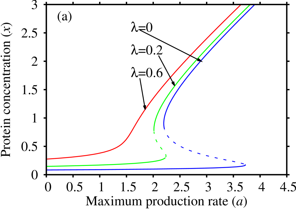
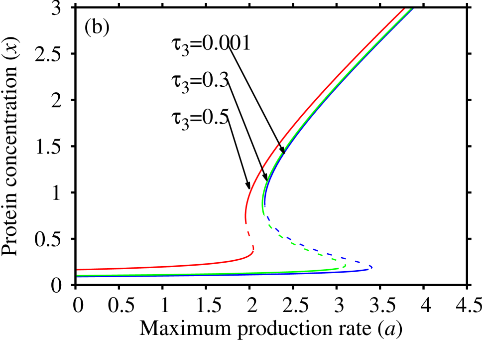
Figure 9: (Color online) Extrema of the SPDF $P_{s}(x)$ of the gene regulation model (6) driven by cross-correlated noises, as a function of $a$: (a) For increasing values of the cross-correlation strength $\lambda$ with other parameter values are $r=0.1$, $\sigma_{1}=0.2$, $\sigma_{2}=0.5$, $\tau_{1}=0.01$, $\tau_{2}=0.01$ and $\tau_{3}=0.1$, and (b) for increasing values of the correlation time $\tau_{3}$ with other parameter values are $r=0.1$, $\sigma_{1}=0.2$, $\sigma_{2}=0.5$, $\tau_{1}=0.5$, $\tau_{2}=0.5$ and $\lambda=0.1$. The bistability regime reduces with increase in both $\lambda$ and $\tau_{3}$.

Using Eq. (14), the extrema of SPDF $P_{s}(x)$ is depicted in Figs. 9(a)-(b) as a function of the maximum transcription rate $a$. Notice that, with increasing values of $\lambda$ and $\tau_{3}$ both extrema curves exhibit similar behavior. As an example, Fig. 9(a) shows that increase in $\lambda$ between two noises reduce the bistability region and for higher values of $\lambda$, bistability completely disappears. These results indicate that correlated stochastic fluctuations in gene regulation can significantly effect the bistable states and even it can reduce it to monostable state. Moreover, the relative stability of the bistable states are dynamically coupled with the correlation parameters of the noise.

III.3 Mean first-passage time of the system driven by cross-correlated noises

For stochastic bistable systems, it is important to estimate the amount of time between shifts from one steady state to another steady state. As it helps to quantify the effects of noise on the regime switching between alternative steady states. This time is often referred as first-passage time. When the first-passage time is averaged over many realizations, the resulting time is called mean first-passage time (MFPT) Ga85 . To examine the robustness of steady states, MFPT provides a very useful characterization. A longer MFPT implies the state is more stable. Now, we study the influence of cross-correlation strength $\lambda$ and correlation time $\tau_{3}$ on the MFPT.

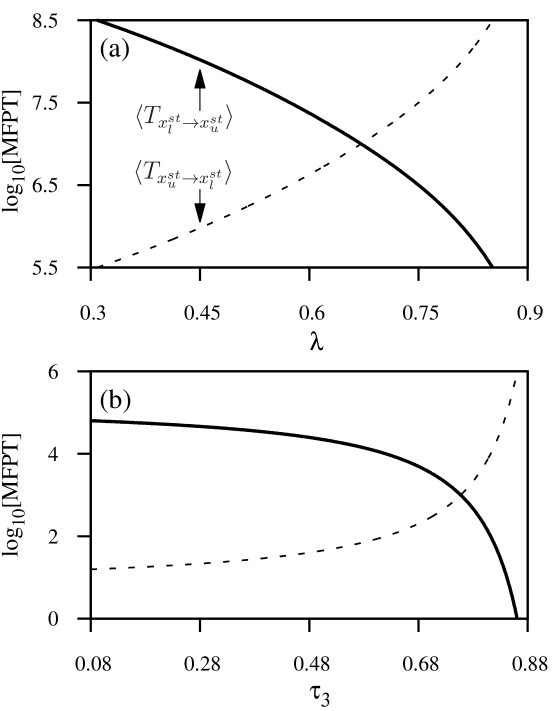
Figure 10: (Color online) The effect of $\lambda$ and $\tau_{3}$ on the MFPT. (a) The MFPT $\langle T_{x_{l}^{st}\rightarrow x_{u}^{st}}\rangle$ decreases and $\langle T_{x_{u}^{st}\rightarrow x_{l}^{st}}\rangle$ increases with the increase of $\lambda$ for $\tau_{3}=0.03$. (b) Similar situation arises with the increase of $\tau_{3}$ for $\lambda=0.3$. The other parameters are same as in Fig. 8.

To start with, let $x_{l}^{st}$ be the low and $x_{u}^{st}$ be the high protein concentration states, separated by a potential barrier $x_{b}^{un}$ (working as a basin boundary between the two steady states $x_{l}^{st}$ and $x_{u}^{st}$) of the system (6). The basin of attraction of the state $x_{u}^{st}$ extends from $x_{b}^{un}$ to $+\infty$, as it is in the right of $x_{l}^{st}$. The MFPT $\langle T(x)\rangle$, can be obtained by solving the following ordinary differential equation Ga85 :

$$A(x)\frac{\partial\langle T\rangle}{\partial x}+\frac{1}{2}B(x)\frac{\partial^{2}\langle T\rangle}{\partial x^{2}}=-1,$$ (21)

with boundary conditions $\langle T(x^{un}_{b})\rangle=0$ and $\frac{\partial\langle T(+\infty)\rangle}{\partial x}=0$, where $A(x)$ and $B(x)$ are respectively given by Eqs. (9a) and (9b).

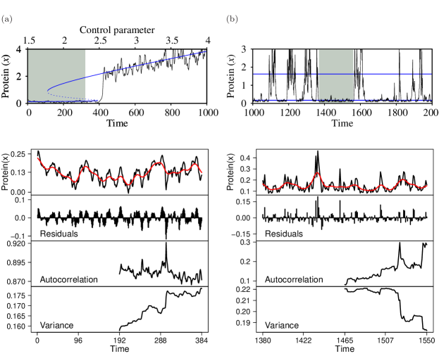
Figure 11: (Color online) Early warning signals for simulated time series data of the stochastic model in the case of: (a) CSD and (b) SS. The variance and autocorrelation are calculated using moving window of half the length of the time series segments (segments are indicated by the shaded regions): (a) For CSD: parameter values are $r=0.1$, $\sigma_{1}=0.002$, $\sigma_{2}=0.09$, $\lambda=0.8$, $\tau_{1}=5$, $\tau_{2}=5$ and $\tau_{3}=1$; (b) For SS: parameter values are $r=0.1$, $a=1.9$, $\sigma_{1}=0.005$ and $\sigma_{2}=0.007$, $\lambda=0.01$, $\tau_{1}=0.09$, $\tau_{2}=0.09$ and $\tau_{3}=1$. The increase in variance act as a robust indicator for CSD, whereas variance fails in the case of SS. The autocorrelation gives weak trend in both CSD and SS.

By solving the Eq. (21), we obtain the expressions of MFPT for $x_{l}^{st}$ and $x_{u}^{st}$. The expressions for MFPT $\langle T_{x_{l}^{st}\rightarrow x_{u}^{st}}\rangle$ and $\langle T_{x_{u}^{st}\rightarrow x_{l}^{st}}\rangle$ are given by Ga85 :

$$\langle T_{x_{l}^{st}\rightarrow x_{u}^{st}}\rangle = 2\int_{x_{l}^{st}}^{x_{b}^{un}}\frac{dy}{\omega(y)}\int_{0}^{y}\frac{\omega(z)}{B(z)}dz,\;\;\text{and}$$ (22)

$$\langle T_{x_{u}^{st}\rightarrow x_{l}^{st}}\rangle = 2\int_{x_{b}^{un}}^{x_{u}^{st}}\frac{dy}{\omega(y)}\int_{y}^{\infty}\frac{\omega(z)}{B(z)}dz,$$ (23)

where

$$w(x)=\exp\Big{(}\int_{x_{0}}^{x}\frac{2A(u)}{B(u)}du\Big{)},$$

with $x_{0}=0$ for the $x_{l}^{st}\rightarrow x_{u}^{st}$ transition and $x_{0}=x_{b}^{u_{n}}$ for the $x_{u}^{st}\rightarrow x_{l}^{st}$ transition.

Effects of changing $\lambda$ and $\tau_{3}$ on the MFPT are shown in Fig. 10. We found that the MFPT $\langle T_{x_{l}^{st}\rightarrow x_{u}^{st}}\rangle$ decreases and $\langle T_{x_{u}^{st}\rightarrow x_{l}^{st}}\rangle$ increases, with increase in the cross-correlation strength $\lambda$ (Fig. 10(a)). Hence, an increase in $\lambda$ results in a regime shift from the left potential well (low concentration state of $x$) to the right potential well (high concentration state of $x$). We observe similar dynamics with variations in $\tau_{3}$ (Fig. 10(b)). The conclusions drawn from the analysis of MFPT are also consistent with the SPDF $P_{s}(x)$ shown in Fig. 8. This result highlights the significance of correlated noise in gene expression dynamics.

III.4 Precursors of regime shift

Here, the main emphasis is to explore the robustness of EWS (e.g., lag-$1$ autocorrelation, variance and conditional heteroskedasticity) as indicators of regime shifts in protein concentration levels. In clinical medicine, EWS can be considered as bio-markers because these are indicators of regime shifts in biological state for living organism ChLi12 . However, earlier techniques or bio-markers are mainly used to investigate the current disease state of an organ based on metabolites or individual protein level Cui2011 ; Jin2009 .

For our analysis, we consider stochastic time series of the model (6) for both the cases, critical slowing down (CSD) and stochastic switching (SS) ScJo09 ; Scheffer:2012sc ; Dakos:2012pone ; sc2015 . The presence of cross-correlated noise in the degradation and basal rates are considered. Numerical simulations have been performed using the Euler-Maruyama method DH01 with an integration step-size of $0.001$. In the time series, we first visually identify shifts between low to high protein concentration. Then we took time series segments (the shaded regions in Fig. 11) prior to a regime shift and analyze them for the presence of EWS. For stationarity in residuals, we used Gaussian detrending with bandwidth 40, before performing any statistical analysis of the data. Then we used a moving window size of half the length of the considered time series segment. The time series analysis have been performed using the “Early Warning Signals Toolbox” (http://www.early-warning-signals.org/). First, we calculate the variance and lag-$1$ autocorrelation, as these two indicators are known to be most appropriate to anticipate regime shifts. The autocorrelation at lag-1 is given by the autocorrelation function (ACF): $\displaystyle\rho_{1}=\frac{E\left[(x(t)-\mu)(x(t+1)-\mu)\right]}{\sigma^{2}}$, where $E$ is the expected value operator, $x(t)$ is the value of the state variable at time $t$, and $\mu$ and $\sigma^{2}$ are the mean and variance of $x(t)$, respectively. Variance is the second moment around the mean $\mu$ and measured as: $\displaystyle\sigma^{2}=\frac{1}{N}\Sigma_{i=1}^{N}(x(t)-\mu)^{2}$, where $N$ is the number of observations within the considered moving window. A concurrent rise in these indicators forewarn an upcoming regime shift Book_Sch ; ScJo09 .

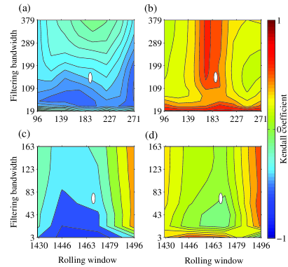
Figure 12: (a) (Color online) Contour plots depict the effects of moving window size and filtering bandwidth on the measured autocorrelation ((a) and (c)) and variance ((b) and (d)) for the: (a-b) CSD data and (c-d) SS data shown in Fig. 11 as estimated by the Kendall’s coefficient. The empty ovals indicate the choices of the window size and filtering bandwidth used in the calculations in Fig. 11.

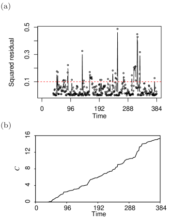
Figure 13: (Color online) CH and cumulative numbers of test estimated on the CSD dataset prior to a regime shift. (a) The squared residuals above the dashed red line are significant. Here, the red line represents the level of significance. (b) The cumulative number $(C)$ of significant Lagrange multiplier test applied to the time series obtained from the model. The number $(C)$ increases prior to the transition indicating that significant number of tests shows conditional heteroskedasticity.

Figure 11(a) shows increase in $\sigma^{2}$ and decrease in $\rho_{1}$ before a regime shift for the case of CSD. Hence, in this case $\sigma^{2}$ is able to successfully detect a regime shift in protein concentration, whereas $\rho_{1}$ fails. However, in the case of SS (Fig. 11(b)), both of these indicators fails. For SS, the failure of $\sigma^{2}$ and $\rho_{1}$ as EWS is in agreement with the previous studies Drake:2013 ; Boet:2013 ; SKP14 ; Sh2016 . The result of EWS analysis also depends on the choice of factors like filtering bandwidth and moving window size, used to calculate the standard deviation and autocorrelation Dakos:2012pone . Hence, it is important to investigate the robustness of our results with respect to the choice of these factors. In particular, we perform sensitivity analysis which is necessary for the selection of bandwidth and moving window size to maximize the estimated trend of EWS. For CSD, we estimate variance and autocorrelation in window size ranging from $25\%$ to $71\%$ (i.e., $96$ to $271$ data points) of the time series length, and for filtering bandwidth ranging from $5\%$ to $100\%$ (see Figs. 12(a) and 12(b)). For SS, we use window size ranging from $25\%$ to $68\%$ (i.e., $1430$ to $1496$ data points) and bandwidth ranging from $2\%$ to $100\%$ (see Figs. 12(c) and 12(d)). Figures 12(a) and 12(c) represent contour plots of rolling window size verses bandwidth for the autocorrelation, similarly Figs. 12(b) and 12(d) for the variance. The empty ovals in Fig. 12 indicate the values those we have used to calculate EWS in Fig. 11. It is clear that the autocorrelation in both the cases CSD (Fig. 12(a)) and SS (Fig. 12(c)) do not give proper result due to the low value of Kendall’s coefficient Dakos:2012pone . However, increasing trend in variance is found in the case of CSD due to the proper selection of window size and bandwidth corresponding to the high value of Kendall’s coefficient, which is also evident from the Fig. 12(b).

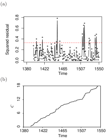
Figure 14: (Color online) CH and cumulative numbers of test estimated on the SS dataset prior to regime shift. (a) The points of CH above the dashed red line are significant. Here, the red line represents the level of significance. (b) The cumulative number $(C)$ of significant Lagrange multiplier test applied to the time series obtained from the model. The number $(C)$ increases prior to the transition indicating that significant number of tests shows CH.

Although autocorrelation and variance are known to be the most preferred indicators to predict regime shifts, the fact is that they are not always successful as shown in the previous examples. This arises because not all the regime shifts are associated with CSD DaCa15 . Moreover, improper data length, statistical limitations and other types of transitions, such as purely noise-induced transitions increase the risk of of false predictions. We cannot avoid the possibility of false alarms completely sc2015 ; DaCa15 . Hence, we further tested another indicator conditional heteroskedasticity (CH) (see Figs. 13 and 14) Se11 . CH is denoted by the persistence in the conditional variance of the error terms. In time series, it looks like as cluster of high variability near a critical transition and cluster of low variability far from the transition. This type of clustering is known to be a leading indicator of regime shifts. CH provides threshold value for detecting regime shift and gives an indication of upcoming regime shift Se11 .

We compute CH using moving window Lagrange multiplier test (window width $10\%$ of the data) Se11 . First we extract the residuals of a fitted model to the time series, then we fit an auto-regressive model of selected order:

$$x_{t}=a_{0}+\sum_{i=1}^{q}a_{i}x_{t-i}+\epsilon_{t},$$

where the order $q$ is selected according to the Akaike information criterion Ak1998 which is a measure of the relative goodness of the fit. Then we squared the residuals $\epsilon_{t}$, and finally the residuals are regressed on themselves lagged by one time step:

$$\epsilon^{2}_{t}=\alpha_{0}+\sum_{i=1}^{q}\alpha_{i}\epsilon^{2}_{t-i},$$

where $\alpha_{0}$ and $\alpha_{i}$ denotes the regression coefficients. The relationship between squared residuals $\epsilon_{t}^{2}$ at lag-1 gives the properties of CH. We also perform chi square test to compare the values of squared residuals to a $\chi^{2}$ distribution to identify the number of significant tests where the CH is observed. The cumulative number of significant tests $(C)$ for CH applied to time series, is expected to increase as the regime shift is approached. Here Fig. 13(a) (Fig. 14(a)) represents the CH estimated on the CSD (SS) dataset prior to a regime shift which shows the positive relationship of error variance and represents the significant CH (i.e., squared residuals) above the significance level. In Figs. 13(a) and Fig. 14(a), the significance level is represented by the red line. The residuals above this red line indicates that there is presence of CH. Figure 13(b) (Fig. 14(b)) shows the result of cumulative number of significant tests $(C)$ for CH applied to time series for the case of CSD (SS) and which is increasing prior to a regime shift and gives positive EWS. It is important to observe that in the case of SS the indicator CH is successful in comparison with autocorrelation and variance and this is evident from Figs. 12 and 14.

IV Discussion

Noise correlation can play a pivotal role in controlling the regulatory functions of gene expression du2008 ; Si2006 ; Ro2005 . In this paper, we have presented theoretical analysis and numerical simulation of a gene expression model to study the role of Gaussian colored noise in inducing sudden regime shifts at the levels of protein concentration. We have used the Ornstein-Uhlenbeck process with the Langevin and Fokker-Plank descriptions to study the effects of Gaussian colored noise. Though one of our main goals is to investigate the effects of noise correlation, for the sake of completeness we also simultaneously studied the effects of colored noise intensity. The theoretical tools used to serve our purpose are the stochastic potential, the stationary probability density function and the mean first-passage time Ga85 . For the presence of colored noise in the protein degradation rate, we have shown that for a fixed correlation time increase in the noise intensity induces regime shift from high (“on” state) to low (“off” state) protein concentration state. Surprisingly, for a fixed noise intensity an increase in the correlation time produces opposite result, it induces regime shift from low (“off” state) to high (“on” state) protein concentration state. Moreover, with the help of the extrema of SPDF we show that for a fixed correlation time, increasing values of noise intensity reduces the bistability regime and for a fixed noise intensity, increasing values of noise correlation increases the bistability regime. Our results also show that colored noise in the basal rate retain the bimodal distribution of the steady states. In the case of cross-correlated colored noises in basal and degradation rates, we have shown that both the cross correlation strength and cross correlation time can induce regime shifts from low to high protein concentration state, but reduce the bistable regime. The results of MFPT for cross-correlated colored noises also matches with the outcome of stochastic potential and SPDF. Thus, unlike earlier studies on gene expression noise Ha00 ; KaEl05 ; Frcasaib12 ; Gh12 ; Sh2016 , our findings suggest that Gaussian colored noise can also induce sudden phenotypic variability (i.e., regime shifts between “on” and “off” expression state) in cells and the noise correlation time can act as a control parameter for that.

Anticipation of regime shifts in gene expression could improve early therapeutic intervention in complex human diseases kor2014 ; gl15 ; Ri2016 . Furthermore, EWS for predicting state shifts in complex biological systems can be very useful as a bio-marker for incurable and chronic human diseases where the stage of the disease is an important factor of therapy and prognosis; for example in liver cancer and lymphoma ChLi12 . Keeping in mind the complexity of cancer, if the stage of cancer can be identified by using EWS, it would be remarkable. Nonetheless, the success of EWS in anticipating catastrophic shifts in ecosystem experiments Wang:2012 suggests that it could be possible to develop and employ EWS in cancer biology based on clinical trials kor2014 ; TrAn15 . Considering, both CSD and SS time series data of the gene expression model we show that variance and autocorrelation sometimes can work as indicators of regime shifts in the levels of protein concentration. However, these indicators can also produce false alarms due to statistical limitations. We also performed sensitivity analysis for the best choice of statistical parameters to be used in time series analysis as to avoid false alarms. When the variance and autocorrelation fails to predict regime shifts, we have shown that other indicator like conditional heteroskedasticity can be successful. The implication of EWS as bio-markers for complex diseases demands experimental verification and is a future challenge for experimental biologists. For predicting regime shifts in gene expression in experiments, one can use single cell flow cytometry measurements which gives rapid analysis of multiple characteristics of single cell Is2003 ; BeHa:2009 . Flow cytometry monitors the distribution of number of proteins in a cell culture.

Further work on extending the kind of analysis presented here to more complex gene networks is needed. Earlier studies in the direction of understanding and predicting regime shifts in gene expression advanced our perception, however there is still lack of quantitative understanding of regime shifts in genetic networks due to its inherent complexity. The main advantage of the mathematical formalism adopted in this paper is that it is simple and easy to understand. We hope that, this reductionist approach could form the basis for more rigorous studies on regime shifts of complex gene networks. Moreover, in this study like many other studies on gene expression we have employed the Langevin and Fokker-Planck description due to their simplicity and analytic tractability Ga85 ; Ha00 ; Gh12 , but one can also use the master equation and its Monte-Carlo simulation Ga85 . Finally, acquiring in depth knowledge about the factors those drive shifts in gene expression states could have significant impact in clinical biology.

- (1) M. Scheffer. Critical transitions in nature and society. Princeton University Press, 2009.
- (2) M. Scheffer, J. Bascompte, W. A. Brock, V. Brovkin, S. R. Carpenter, V. Dakos, H. Held, E. H van Nes, M. Rietkerk, and G. Sugihara. Early-warning signals for critical transitions. Nature, 461:53–59, 2009.
- (3) M. Scheffer, S. R. Carpenter, J. A. Foley, C. Folke, and B. Walker. Catastrophic shifts in ecosystems. Nature, 413:591–596, 2001.
- (4) M. Scheffer and S. R. Carpenter. Catastrophic regime shifts in ecosystems: linking theory to observation. Trends in Ecology & Evolution, 18(12):648–656, 2003.
- (5) R. Wang, J. A. Dearing, P. G. Langdon, E. Zhang, X. Yang, V. Dakos, and M. Scheffer. Flickering gives early warning signals of a critical transition to a eutrophic lake state. Nature, 492:419–422, 2012.
- (6) T. M. Lenton, H. Held, E. Kriegler, J. W. Hall, W. Lucht, S. Rahmstorf, and H. J. Schellnhuber. Tipping elements in the earth’s climate system. Proceedings of the National Academy of Sciences USA, 105(6):1786–1793, 2008.
- (7) J. G. Venegas, T. Winkler, G. Musch, M.F.V. Melo, D. Layfield, N. Tgavalekos, A.J. Fischman, R.J. Callahan, G. Bellani, and G. Bellani. Self-organized patchiness in asthma as a prelude to catastrophic shifts. Nature, 434:777–782, 2005.
- (8) P. E. McSharry, L. A. Smith, and L. Tarassenko. Prediction of epileptic seizures: are nonlinear methods relevant? Nature Medicine, 9:241–242, 2003.
- (9) K. S. Korolev, J. B. Xavier, and J. Gore. Turning ecology and evolution against cancer. Nature Reviews Cancer, 14(5):371–380, 2014.
- (10) M. G. O. Rikkert, V. Dakos, T. G. Buchman, R. de Boer, L. Glass, A. O. Cramer, S. Levin, E. van Nes, G. Sugihara, M. D. Ferrari, and E. A. Tolner. Slowing down of recovery as generic risk marker for acute severity transitions in chronic diseases. Critical Care Medicine, 44(3):601–606, 2016.
- (11) R. M. May, S. A. Levin, and G. Sugihara. Complex systems: Ecology for bankers. Nature, 451:893–895, 2008.
- (12) J. M. Fox and G. M. Whitesides. Warning signals for eruptive events in spreading fires. Proceedings of the National Academy of Sciences USA, 112(8):2378–2383, 2015.
- (13) E. A. Gopalakrishnan, Y. Sharma, T. John, P. S. Dutta, and R. I. Sujith. Early warning signals for critical transitions in a thermoacoustic system. Scientific Reports, 6:35310, 2016.
- (14) M. Scheffer, S. R. Carpenter, T. M. Lenton, J. Bascompte, W. A. Brock, V. Dakos, J. van de Koppel, I. A. van de Leemput, S. A. Levin, E. H. van Nes, M. Pascual, and J. Vandermeer. Anticipating critical transitions. Science, 338:344–348, 2012.
- (15) V. Dakos, S. R. Carpenter, E. H. van Nes, and M. Scheffer. Resilience indicators: prospects and limitations for early warnings of regime shifts. Philosophical Transactions of the Royal Society B: Biological Sciences, 370:20130263, 2015.
- (16) Y. Sharma, K. C. Abbott, P. S. Dutta, and A. K. Gupta. Stochasticity and bistability in insect outbreak dynamics. Theoretical Ecology, 8:163–174, 2015.
- (17) Y. Sharma, P. S. Dutta, and A. K. Gupta. Anticipating regime shifts in gene expression: The case of an autoactivating positive feedback loop. Physical Review E, 93(3):032404, 2016.
- (18) V. Dakos, S. R. Carpenter, W. A. Brock, A. M. Ellison, V. Guttal, A. R. Ives, S. Kéfi, V. Livina, D. A. Seekell, E. H. van Nes, and M. Scheffer. Methods for Detecting Early Warnings of Critical Transitions in Time Series Illustrated Using Simulated Ecological Data. PLoS One, 7:e41010, 2012.
- (19) S. R. Carpenter, W. A. Brock, J. J. Cole, J. F. Kitchell, and M. L. Pace. Leading indicators of trophic cascades. Ecology Letters, 11:128–138, 2008.
- (20) V. Guttal and C. Jayaprakash. Changing skewness: an early warning signal of regime shifts in ecosystems. Ecology Letters, 11:450–460, 2008.
- (21) M. Scheffer, S. R. Carpenter, V. Dakos, and E. H. van Nes. Generic indicators of ecological resilience: inferring the chance of a critical transition. Annual Review of Ecology, Evolution, and Systematics, 46:145–167, 2015.
- (22) D. A. Seekell, S. R. Carpenter, and M. L. Pace. Conditional heteroscedasticity as a leading indicator of ecological regime shifts. The American Naturalist, 178:442–451, 2011.
- (23) R. F. Engle. Autoregressive conditional heteroscedasticity with estimates of the variance of united kingdom inflation. Econometrica: Journal of the Econometric Society, 50(4):987–1007, 1982.
- (24) M. Pal, A. K. Pal, S. Ghosh, and I. Bose. Early signatures of regime shifts in gene expression dynamics. Physical Biology, 10(3):036010, 2013.
- (25) L. Glass. Dynamical disease: Challenges for nonlinear dynamics and medicine. Chaos: An Interdisciplinary Journal of Nonlinear Science, 25:097603, 2015.
- (26) C. Trefois, P. M. Antony, J. Goncalves, A. Skupin, and R. Balling. Critical transitions in chronic disease: transferring concepts from ecology to systems medicine. Current Opinion in Biotechnology, 34:48–55, 2015.
- (27) L. Chen, R. Liu, Z-P. Liu, M. Li, and K. Aihara. Detecting early-warning signals for sudden deterioration of complex diseases by dynamical network biomarkers. Scientific Reports, 2:342, 2012.
- (28) I. A. van de Leemput, M. Wichers, A. O. Cramer, D. Borsboom, F. Tuerlinckx, P. Kuppens, E. H. van Nes, W. Viechtbauer, E. J. Giltay, S. H. Aggen, and C. Derom. Critical slowing down as early warning for the onset and termination of depression. Proceedings of the National Academy of Sciences USA, 111(1):87–92, 2014.
- (29) J. Lagro, N. C. Laurenssen, B. W. Schalk, Y. Schoon, J. A. Claassen, and M. G. O. Rikkert. Diastolic blood pressure drop after standing as a clinical sign for increased mortality in older falls clinic patients. Journal of Hypertension, 30(6):1195–1202, 2012.
- (30) M. A. Kramer, W. Truccolo, U. T. Eden, K. Q. Lepage, L. R. Hochberg, E. N. Eskandar, J. R. Madsen, J. W. Lee, A. Maheshwari, E. Halgren, C. J. Chu, and S. S. Cash. Human seizures self-terminate across spatial scales via a critical transition. Proceedings of the National Academy of Sciences USA, 109(51):21116–21121, 2012.
- (31) M. Scheffer, A. van den Berg, and M. D. Ferrari. Migraine strikes as neuronal excitability reaches a tipping point. PLoS One, 8(8):e72514, 2013.
- (32) P. Smolen, D. A. Baxter, and J. H. Byrne. Frequency selectivity, multistability, and oscillations emerge from models of genetic regulatory systems. American journal of Physiology, 274:C531–C542, 1998.
- (33) M. Kaern, T. C. Elston, W. J. Blake, and J. J. Collins. Stochasticity in gene expression: from theories to phenotypes. Nature Reviews Genetics, 6:451–464, 2005.
- (34) J. Hasty, J. Pradines, M. Dolnik, and J. J. Collins. Noise-based switches and amplifiers for gene expression. Proceedings of the National Academy of Sciences USA, 97:2075–2080, 2000.
- (35) Q. Liu and Y. Jia. Fluctuations-induced switch in the gene transcriptional regulatory system. Physical Review E, 70:041907, 2004.
- (36) Z. Cheng, F. Liu, X. Zhang, and W. Wang. Robustness analysis of celular memory in an autoactivating positive feedback system. FEBS Letters, 582:3776––3782, 2008.
- (37) D. Frigola, L. Casanellas, J. M. Sancho, and M. Ibañes. Asymmetric stochastic switching driven by intrinsic molecular noise. PLoS One, 7:e31407, 2012.
- (38) S. Ghosh, S. Banerjee, and I. Bose. Emergent bistability: Effects of additive and multiplicative noise. The European Physical Journal E, 35(2):1–14, 2012.
- (39) N. Rosenfeld, J. W. Young, U. Alon, P. S. Swain, and M. B. Elowitz. Gene regulation at the single-cell level. Science, 307(5717):1962–1965, 2005.
- (40) A. Sigal, R. Milo, A. Cohen, N. Geva-Zatorsky, Y. Klein, Y. Liron, N. Rosenfeld, T. Danon, N. Perzov, and U. Alon. Variability and memory of protein levels in human cells. Nature, 444(7119):643–646, 2006.
- (41) V. Shahrezaei, J. F. Ollivier, and P. S. Swain. Colored extrinsic fluctuations and stochastic gene expression. Molecular Systems Biology, 4(1):196, 2008.
- (42) M. J. Dunlop, R. S. Cox, J. H. Levine, R. M. Murray, and M. B. Elowitz. Regulatory activity revealed by dynamic correlations in gene expression noise. Nature Genetics, 40(12):1493–1498, 2008.
- (43) M. J. Dunlop. Dynamics and Correlated Noise in Gene Regulation. PhD thesis, California Institute of Technology, Pasadena, California, 2008.
- (44) M. M. Klosek-Dygas, B. J. Matkowsky, and Z. Schuss. Colored noise in dynamical systems. SIAM Journal on Applied Mathematics, 48(2):425–441, 1988.
- (45) A. Becksei, B. Seraphin, and L. Serrano. Positive feedback in eukaryotic gene networks: cell differentiation by graded to binary response. The EMBO, 20:2528––2535, 2001.
- (46) J. J. Tyson, K. C. Chen, and B. Novak. Sniffers, buzzers, toggles and blinkers: dynamics of regulatory and signaling pathways in the cell. Current Opinion in Cell Biology, 15:221––231, 2003.
- (47) F. J Isaacs, J. Hasty, C. R. Cantor, and J. J. Collins. Prediction and measurement of an autoregulatory genetic module. Proceedings of the National Academy of Sciences USA, 100(13):7714–7719, 2003.
- (48) M. Thattai and A. Van Oudenaarden. Intrinsic noise in gene regulatory networks. Proceedings of the National Academy of Sciences USA, 98(15):8614–8619, 2001.
- (49) X. Zheng and X. Yang and Y. Tao. Bistability, probability transition rate and first-passage time in an autoactivating positive-feedback loop. PLoS One, 6:e17104, 2011.
- (50) C. V. Rao and A.P. Arkin. Stochastic chemical kinetics and the quasi-steady-state assumption: application to the gillespie algorithm. The Journal of Chemical Physics, 118(11):4999–5010, 2003.
- (51) M. Weber and J. Buceta. Stochastic stabilization of phenotypic states: The genetic bistable switch as a case study. PLoS One, 7:e73487, 2013.
- (52) C. W. Gardiner. Handbook of Stochastic Methods: For Physics, Chemistry and the Natural Sciences. Springer–Verlag, Berlin, 2nd edition, 1985.
- (53) J. M. Sancho, M. San Miguel, S. L. Katz, and J. D. Gunton. Analytical and numerical studies of multiplicative noise. Physical Review A, 26(3):1589, 1982.
- (54) G. Y. Liang, L. Cao, and D. J. Wu. Approximate fokker–planck equation of system driven by multiplicative colored noises with colored cross-correlation. Physica A: Statistical Mechanics and its Applications, 335(3):371–384, 2004.
- (55) W. Horsthemke and R. Lefever. Noise-Induced Transitions. Springer, Berlin, 1984.
- (56) S. Rothman. How is the balance between protein synthesis and degradation achieved? Theoretical Biology and Medical Modelling, 7(1):1, 2010.
- (57) J. Cui, Y. Chen, W.C. Chou, L. Sun, L. Chen, J. Suo, Z. Ni, M. Zhang, X. Kong, L.L. Hoffman, and J. Kang. An integrated transcriptomic and computational analysis for biomarker identification in gastric cancer. Nucleic acids research, 39(4):1197–1207, 2011.
- (58) G. Jin, X. Zhou, K. Cui, X.S Zhang, L. Chen, and S.T.C Wong. Cross-platform method for identifying candidate network biomarkers for prostate cancer. IET Systems Biology, 3(6):505–512, 2009.
- (59) D. J. Higham. An algorithmic introduction to numerical simulation of stochastic differential equations. SIAM Review, 43(3):525–546, 2001.
- (60) J. M Drake. Early warning signals of stochastic switching. Proceedings of the Royal Society of London B: Biological Sciences, 280(1766):20130686, 2013.
- (61) C. Boettiger and A. Hastings. No early warning signals for stochastic transitions: insights from large deviation theory. Proceedings of the Royal Society of London B: Biological Sciences, 280(1766):20131372, 2013.
- (62) H. Akaike. Information theory and an extension of the maximum likelihood principle. In Selected Papers of Hirotugu Akaike, pages 199–213. Springer, 1998.
- (63) M. Bennett and J. Hasty. Microfluidic devices for measuring gene network dynamics in single cells. Nature Reviews Genetics, 10:628–638, 2009.