Deep CFHT $Y$-band imaging of VVDS-F22 field: I.
data products and photometric redshifts

Abstract

We present our deep $Y$-band imaging data of a two square degree field within the F22 region of the VIMOS VLT Deep Survey. The observations were conducted using the WIRCam instrument mounted at the Canada–France–Hawaii Telescope (CFHT). The total on-sky time was 9 hours, distributed uniformly over 18 tiles. The scientific goals of the project are to select faint quasar candidates at redshift $z>2.2$, and constrain the photometric redshifts for quasars and galaxies. In this paper, we present the observation and the image reduction, as well as the photometric redshifts that we derived by combining our $Y$-band data with the CFHTLenS $u^{*}g^{\prime}r^{\prime}i^{\prime}z^{\prime}$ optical data and UKIDSS DXS $JHK$ near-infrared data. With $J$-band image as reference total $\sim$ 80,000 galaxies are detected in the final mosaic down to $Y$-band $5\sigma$ point source limiting depth of 22.86 mag. Compared with the $\sim$ 3500 spectroscopic redshifts, our photometric redshifts for galaxies with $z<1.5$ and $i^{\prime}\lesssim 24.0$ mag have a small systematic offset of $|\Delta{z}|\lesssim 0.2$, 1$\sigma$ scatter $0.03<\sigma_{\Delta z}<0.06$, and less than 4.0% of catastrophic failures. We also compare to the CFHTLenS photometric redshifts, and find that ours are more reliable at $z\gtrsim 0.6$ because of the inclusion of the near-infrared bands. In particular, including the $Y$-band data can improve the accuracy at $z\sim 1.0-2.0$ because the location of the 4000Å-break is better constrained. The $Y$-band images, the multi-band photometry catalog and the photometric redshifts are released at http://astro.pku.edu.cn/astro/data/DYI.html.

1 Introduction

Surveys in optical to near-infrared are vital in astronomy. Due to the characteristics of detector response, the conventional charge coupled devices (CCD) used for optical surveys are mostly sensitive at $\lambda\lesssim 0.9\,\mu$m (e.g., the Sloan Digital Sky Survey, SDSS; York et al. (2000)), while the detectors, such as hybrid HgCdTe arrays, for near-infrared surveys normally work at $\lambda\gtrsim 1.0\,\mu$m (e.g., 2-Micron All Sky Survey, 2MASS; Skrutskie et al. (2006)). This leaves a gap of $\sim$ 0.1 $\mu$m in between. The development in detector technology in the past decade has allowed this gap to be gradually bridged by extending from both optical and near-infrared. Nowadays imaging in this regime is usually done through a broadband filter designated as “$Y$”, noting that the shape and amplitude of the spectral response of CCDs in the $Y$-band are not identical to their counterparts with near-infrared detectors because of the different structures and fabrications. Surveys incorporating $Y$-band are now routinely carried out. Some recent examples include the Dark Energy Survey (DES; Sánchez et al. (2014)) extending from optical to $Y$ and the UKIDSS Large Area Survey (LAS; Dye et al. (2006); Lawrence et al. (2007)) from $JHK$ to $Y$. The uniqueness of $Y$ band has enriched astronomical studies, such as the refinement of quasar selection (Wu & Jia, 2010) and improving photometric redshift measurements (Ilbert et al., 2009; Sánchez et al., 2014).

Quasars play important roles in studying a variety of subjects ranging from the large-scale structure of the Universe to the evolution of galaxies. Being the extreme of active galactic nuclei (AGN), quasars are rare objects in the Universe. Thus for quasar studies, an important aspect is to refine the candidate selection method such that the final sample can be as complete as possible with a low false detection rate at the same time. In this regard, the quasar selection in SDSS is highly successful (see e.g. Richards et al. (2002)). However, it becomes severely incomplete at $z>2.2$. To mitigate this problem, a “$K$-band excess method” has been proposed (Warren et al., 2000; Hewett et al., 2006; Maddox et al., 2008).

In this paper, we present the Deep $Y$-band Imaging project (hereafter DYI; PI: X.-B. Wu), which used the CFHT Wide-field InfraRed Camera (WIRCam; Puget et al. (2004)) to image a two square degree area within the VVDS-F22 field. The main scientific aims are to select faint quasar candidates using the color criteria proposed by Wu & Jia (2010) and to study if the photometric redshift measurements for quasars and galaxies can be improved. VVDS-F22 is a contiguous field of VVDS-Wide survey, covering 4 square degrees (Garilli et al., 2008; Le Fèvre et al., 2013). It is also covered by SDSS Stripe 82 (Annis et al., 2014), CFHT Legacy Survey (CFHTLS), UKIDSS LAS and Deep Extragalactic Survey (DXS), and NRAO Very Large Array Sky Survey (NVSS; Condon et al. (1998)). Over 100 quasars at 0.5 $<z<$ 4.7 within this field have been spectroscopically identified by SDSS and VVDS, and almost all of them (except one) satisfy the color-color selection criteria. The DYI photometry, reaching $5\sigma$ point source limiting magnitude of 22.86 mag, is 2.0 mag and 1.5 mag deeper than that of UKIDSS LAS and VISTA Hemisphere Survey (VHS; Cross et al. (2012)), respectively, and is comparable to the UKIDSS DXS $K$-band depth.

In addition to quasar selections (Yang et al., in preparation), our $Y$-band data can also be important in improving the photometric redshift measurements of the galaxies with $z\sim 1.25-1.8$ in the field, because the 4000Å-break, one of the most prominent spectral features that photometric redshift estimate could rely on (e.g. Ilbert et al. (2009); Laigle et al. (2016)), moves to $Y$-band at these redshifts. Many ongoing and upcoming wide field surveys, especially those for weak lensing studies, include $Y$-band observations in order to improve photometric redshift accuracy beyond $z\sim 1.0$, such as DES, the Large Synoptic Survey Telescope (LSST; LSST Science Collaboration et al. (2009)), and the Euclid mission (Laureijs et al., 2011). As an example, the CFHT Lensing Survey (CFHTLenS; Heymans et al. (2012) & Erben et al. (2013)) can only obtain robust photometric redshifts ($0.03<\sigma<0.06$) in the range $0.1<z<1.3$ using five optical $u^{*}g^{\prime}r^{\prime}i^{\prime}z^{\prime}$ bands (Hildebrandt et al., 2012). The LSST, on the other hand, is expected to reach $\sigma\sim 0.02$ over $0<z<3$, and one of the main reasons that enable such an accuracy at $z<2$ is the inclusion of $Y$-band.

Reduction of ground-based $Y$-band data, however, is non-trivial (Ramsay et al., 1992; High et al., 2010). In this paper, we present the DYI observation and image reduction. We also show the photometric redshift measurements for galaxies in combination with CFHTLenS and UKIDSS DXS imaging data. In particular, we analyze the impact of $Y$-band photometry on photometric redshift measurements.

The paper is organized as follows. In Section 2, we introduce the observations of our DYI project. The detailed data reduction procedures are presented in Section 3. In Section 4, we describe the multi-band photometry and the treatment of the PSF inhomogeneity between different band images. We present the derivation of photometric redshifts for galaxies and the analysis of their accuracy in Section 5. Summaries are presented in Section 6. Note that all magnitudes in this paper are in the AB system. The conversion constants between the Vega and AB magnitudes for UKIDSS $YJHK$ bands are from Hewett et al. (2006).

2 Observation

The DYI project was conducted during August to October 2012 using the WIRCam instrument mounted on CFHT. The WIRCam focal plane is made of a mosaic of four HAWAII2-RG detectors, each containing $2048\times 2048$ pixels, with a sampling of $0.3\arcsec$ per pixel. Each detector is read in parallel using 32 amplifiers. The detectors are operated at $\sim$ 80 Kelvin with the readout noise of $\sim$ 30 e^- and very low dark current ($\sim$ 0.05 e^-/sec). The average electronic gain is 3.8 e^-/ADU. The field of view of the full mosaic is about $21.5\arcmin\times 21.5\arcmin$. The whole DYI field was divided into 18 uniform tiles, each $20\arcmin\times 20\arcmin$ in size. Figure 1 shows this layout on top of the final mosaic, which amounts to $128\arcmin\times 65\arcmin$. Blue crosses indicate the positions of galaxies with reliable spectroscopic redshifts. Our observation, carried out in Queue Service Observing mode (QSO), took place over two periods: one was in August with single exposure time of 127.5 seconds, and the other spanned the period from September to October with single exposure of 115.0 seconds. The total exposure time of each tile is about 0.5 hour.

For each tile we requested 16 dithered exposures in order to fill the $45\arcsec$ inner gaps between the detectors. In addition, the dither mode can not only improve the spatial sampling, but also avoid the detector defects (e.g., the bad pixels) and efficiently remove cosmic rays and the high sky background. Figure 2 shows the dither pattern for the tile F2218+0030 with magenta dots denoting the central celestial coordinates of the 16 exposures. The arrows in the figure indicate the dither directions and amplitudes between two adjacent exposures. On average the dither shift of each tile is about $1.8\arcmin$.

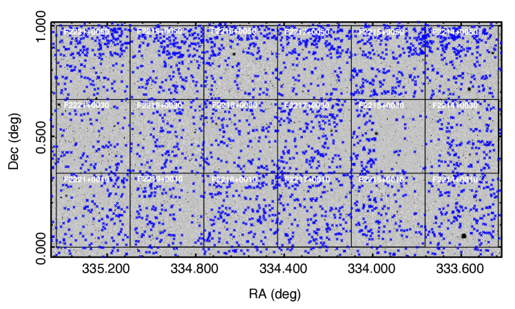
Figure 1: Sky coverage ($128\arcmin\times 65\arcmin$) of the final, stacked $Y$-band image. The 18 tiles, each $20\arcmin\times 20\arcmin$ in size, are overlaid as the thin, black grids. Blue crosses indicate the positions of galaxies with spectroscopic redshifts. The background image is shown with inverted grey scale, and the large black points represent the saturated stars.

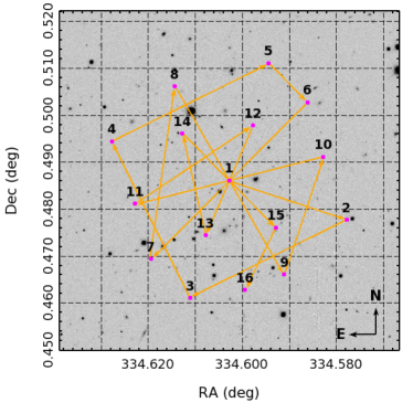
Figure 2: The dither pattern of the tile F2218+0030. The mosaic shows the inner $4.3\arcmin\times 4.3\arcmin$ area centered at the first exposure. The magenta dots represent the central positions of the 16 dithered exposures, while the arrows indicate the dither directions and amplitudes between two adjacent exposures.

3 Image Reduction

The WIRCam images are graded at five levels based on the seeing condition, sky background, timing etc., and we only use Grade 1 and 2 images, which are good for scientific purpose. The raw images were preprocessed by ’I’iwi pipeline (version 2.0), including flagging the saturated pixels, non-linearity correction, reference pixels subtraction, dark subtraction, flat fielding, bad pixels and guide window masking, and basic cross-talk removal. In the following work, we will concentrate on these preprocessed images, referred as science images. We note that ’I’iwi pipeline also provided the sky subtracted images, but in this work we perform the sky subtraction using our own method. Table 1 summarizes the basic observational information. The exposure time of each tile used in the work is listed in the seventh column. These exposures are selected to be continuous to ensure that the seeing does not vary too much. The seeing is the median value of all useful exposures, ranging from 0.56$\arcsec$ to 1.18$\arcsec$. We note that almost one third of the images have seeing larger than 1.0″. For the sake of sensitivity, we do not further reject the science images on the basis of their seeing values. Three tiles, F2215+0050, F2217+0050 and F2218+0050, were observed under thin cirrus, but this did not affect their photometric zeropoint determination when following the same reduction procedures as other photometric tiles. Therefore, they are included in our process.

3.1 Cosmic Rays and Satellite Track Removal

Even with 16 exposures, the rejection of defects such as cosmic rays could still be non-optimal if we rely on the conventional algorithm such as sigma-clipping. To get the best co-adds, we opt to remove such defects from the single images as much as possible.

The cosmic rays are detected and removed. This is done by a Python code that implements the L.A. Cosmic algorithm, which is based on a variant of Laplacian edge detection (van Dokkum, 2001). The method is capable of rejecting cosmic rays of arbitrary shape by applying a 2D Laplacian convolution kernel which is sensitive to variations on small scales. In addition, saturated stars and their full saturation trails can also be flagged by the module automatically. In some cases, however, it misclassifies the peaks of unsaturated bright stars as cosmic rays. We modify the module to suite the work and find the best parameters by visual inspection of the mask images. The rejection is done through three iterations, and the results are satisfactory.

In general, the sky background dominates the near-infrared images so that the satellite trails are relatively too faint to be detected. Instead, we identify the satellite trails from the sky subtracted images produced by ’I’iwi pipeline and then mask them from the science images.

Table 1: Summary of Our DYI Project.

Field ID	R.A.	Dec.	Month, Year	Ntot	Neff	Expeff	Seeing
	(J2000)	(J2000)				(s)	($\arcsec$)
F2214+0010	22:14:28	+00:10:00	Aug.-Sep.,2012	16	16	1840.0	0.74
F2214+0030	22:14:28	+00:30:00	Oct.,2012	16	16	1840.0	1.07
F2214+0050	22:14:28	+00:50:00	Oct.,2012	18	16	1840.0	1.09
F2215+0010	22:15:48	+00:10:00	Aug.,2012	19	7	892.5	0.57
F2215+0030	22:15:48	+00:30:00	Aug.,2012	16	16	2040.0	0.79
F2215+0050	22:15:48	+00:50:00	Sep.,2012	16	11	1402.5	0.70
F2217+0010	22:17:08	+00:10:00	Aug.,2012	16	16	2040.0	0.56
F2217+0030	22:17:08	+00:30:00	Aug.,2012	16	16	2040.0	0.79
F2217+0050	22:17:08	+00:50:00	Sep.,2012	16	16	2040.0	0.80
F2218+0010	22:18:28	+00:10:00	Aug.,2012	16	16	2040.0	0.57
F2218+0030	22:18:28	+00:30:00	Aug.,2012	16	16	2040.0	0.75
F2218+0050	22:18:28	+00:50:00	Sep.,2012	10	7	892.5	0.75
F2219+0010	22:19:48	+00:10:00	Oct.,2012	15	13	1495.0	1.15
F2219+0030	22:19:48	+00:30:00	Oct.,2012	16	14	1610.0	0.78
F2219+0050	22:19:48	+00:50:00	Oct.,2012	16	15	1725.0	0.74
F2221+0010	22:21:08	+00:10:00	Oct.,2012	16	16	1840.0	0.67
F2221+0030	22:21:08	+00:30:00	Oct.,2012	16	16	1840.0	1.18
F2221+0050	22:21:08	+00:50:00	Oct.,2012	16	16	1840.0	1.15

Note. — The fifth column shows the number of raw exposures of each tile, while the sixth column N_eff represents the number of images with GRADE 1 and 2. The total exposure time of each tile used in the work is listed under Exp_eff. The quoted seeing value in the last column is the median of all good exposures. Three fields, 2215+0050, 2217+0050 and 2218+0050, were observed under non-photometric condition.

3.2 Sky Background Subtraction

Due to the OH emission lines, the $Y$-band sky background varies rapidly, at a time scale of a few minutes to an hour (Ramsay et al., 1992; High et al., 2010). As a compromise between the limited exposure times and the temporal variations of the sky, we perform the background subtraction on images with continuous exposure time no more than 15 minutes for each tile. Therefore, if the exposure is longer than that, the tile will be divided into two roughly uniform groups.

For each group, we run SExtractor (version 2.19.5; Bertin & Arnouts (1996)) to create the preliminary background subtracted images. Then they are integer-registered to a common grid by matching dozens of stars with high signal-to-noise ratios, and stacked to an intermediate image. All objects are extracted from the stacked image by applying a low detection threshold and masked from the original science images. In general, the background values of the mask regions can be estimated by two dimensional interpolation with nearby pixels. However, it leads to some obvious artificial features in the large mask regions, especially at the positions of bright objects. Moreover, performing two dimensional interpolation is relatively time-consuming. For a small blank region in the image, we find that the distribution of the pixel values can be well fitted by a Gaussian function. Therefore, for a specific mask region, the median value $\bf{a}$ and variance $\bf{\sigma^{2}}$ are calculated through its adjacent pixels (at least 900 unmasked pixels) to construct a Gaussian pseudo-random number generator following distribution $N(\bf{a},\bf{\sigma^{2}})$. The masked pixels are filled with random numbers sampled by the generator. This procedure conserves the local statistical properties, and avoids many artificial effects due to the interpolation. Finally, the background map of a certain exposure is created by a running median of all other masked images. As an example, for a group having 8 exposures, the background map of the third exposure is created by combing other seven exposures. During the procedure, we apply $3\sigma$-clipping to reject the bad pixels.

3.3 Other systematics Removal

After the background subtraction, the images still show visible systematics that appear as horizontal stripes because of the residual amplifier differences. Similar to Muñoz et al. (2014), we take the median along the $x$-axis for the pixels belonging to a given amplifier. The variation is smoothed and fitted with a linear equation. We estimate the best fitted coefficients through least squares method and subtract this trend from the images.

We do not see any obvious large scale variations in the images as mentioned by Muñoz et al. (2014). However, the images of the forth detector indeed show very small inhomogeneities, and the patterns are not constant between different exposures. The amplitude is indistinguishable from the variance of the background noise so that it is not expected to affect the photometry. Therefore, we do not further take the inhomogeneities into account.

3.4 Astrometric and Photometric Calibrations

We use SCAMP (version 2.2.6, Bertin (2006)) for astrometric calibration with 2MASS point source catalog as reference. To find the accurate astrometric solution, the SCAMP is run twice. We consider the detector positions to be independent between exposures (MOSAIC_TYPE = LOOSE) for the first time. In that case, the astrometric calibration is conducted separately for each exposure. Then we run SCAMP again to derive a common and median relative positioning of the four detectors within the focal plane (MOSAIC_TYPE = FIX_FOCALPLANE). The final derived pixel scale varies radially in a symmetric way by 0.6% from the center to the edge of the field of view. The rms offsets of the astrometry, comparing with the 2MASS world coordinates, are less than 0.14$\arcsec$ along both right ascension and declination axes.

Because the DYI field has been covered by UKIDSS LAS $Y$ band (hereafter $Y_{\mathrm{LAS}}$), we use its photometry as reference to perform photometric calibration. The SDSS Stripe 82 standard star catalog (Ivezić et al., 2007) is cross-matched with $Y_{\mathrm{LAS}}$-band catalog to get the $Y_{\mathrm{LAS}}$-band magnitudes. We further constrain the stars to have signal-to-noise ratios larger than 10 in $Y_{\mathrm{LAS}}$ band (corresponding magnitudes brighter than 19.0 mag). In total, there are about 2500 stars that uniformly distribute in the field.

The effective wavelength and bandpass of $Y_{\mathrm{LAS}}$ band are 1.03 $\mu$m and 0.1 $\mu$m, respectively. Though it is quite similar to WIRCam $Y$ band, we also derive a color correction between the two bands by including UKIDSS LAS $J$ band in order to avoid any potential magnitude bias. The Pickles star spectra library (Pickles, 1998) is used to calculate the convolutional magnitude. The linear color relation can be written as

$$Y-Y_{\text{LAS}}=0.0342\times(Y-J)_{\text{LAS}}+0.0042$$ (1)

with rms scatter of 0.004 mag. As expected, the coefficients in the color relation are very small and the color correction is at most 0.03 mag. Then we determine the zeropoint by the equation

$$m_{\text{zp}}=m_{Y}+2.5\times\log{f}+c-\alpha\times{k_{\nu}},$$ (2)

where $m_{Y}$ represents the apparent $Y$-band magnitude of each star and $f$ is the corresponding observed flux in unit of $\mathrm{ADU\,s^{-1}}$. The parameter $c$ is the color correction term in equation (1) and $\alpha$ and $k_{\nu}$ are the airmass and corresponding coefficient. To determine $k_{\nu}$, we extrapolate the Extinction Curve of Mauna Kea from the recent results by Buton et al. (2013) to 1.0 $\mu$m.

However, we note that the zeropoints are different between the four WIRCam detectors due to the different gain values, as also pointed out by Muñoz et al. (2014) when analyzing $K_{s}$-band images. The offsets can be as large as 0.1 mag. Therefore, we do photometric calibration for each detector separately, and then correct the offsets to a common zeropoint. Specifically, for a certain tile we run firstly SCAMP on the images of each detector to homogenize the flux scales (i.e. parameter FLXSCALE in headers). SWarp (version 2.38.0; Bertin et al. (2002)) is then used to median stack the images with resampled pixel scale of $0.3\arcsec$. We extract the source catalog by SExtractor and cross match with the reference star catalog. The median value of the differences between the instrumental and apparent magnitudes is calculated as the detector’s zeropoint. Finally, we set the zeropoints of the four detectors to 24.30 mag by rescaling the flux scale parameter in the image headers.

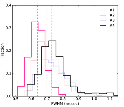
Figure 3: Fractional FWHM histograms of the four detectors for tile F2217+0010. Vertical dashed lines indicate the median FWHM values. To emphasize the difference between detector 2 and 4, the color contrasts of the other two detectors are downweighted. The FWHM is estimated by SExtractor for stars with signal-to-noise ratios larger than 20.

3.5 Image Stacking and Photometric Quality

We stack the background subtracted images using SWarp in combination with the astrometric and photometric calibrated headers calculated by SCAMP. However, after stacking all the images into one mosaic for a certain tile, the distribution of the full width at half maximum (FWHM) of stars shows either multiple peaks or large dispersion of over $0.3\arcsec$. This problem will definitely bias the aperture photometry. By checking the FWHM distribution of the mosaic for each detector, however we find that it is well behaved which shows small variation, typically within $0.2\arcsec$. In other words, the FWHM distributions are slightly different between the detectors. As a result, it leads to the FWHM distribution of the stacked image having multiple peaks or large dispersion. The difference presumably results from the different responses of the four detectors, the dither mode, or the image stacking procedures. However, for the last two cases, it is not supposed to see any deviation from the FWHM distributions of individual exposures. Therefore, we count the FWHM values of stars in every single exposure, and then analyze their statistical distributions, by combining these values of all exposures, of the four detectors individually. Figure 3 shows an example for tile F2217+0010. The FWHM is estimated by SExtractor for stars with signal-to-noise ratios larger than 20. From the figure we can see clear deviations even in the individual exposures, of which the median offset between detector 2 and 4 is nearly $0.1\arcsec$. Further, we calculate the median FWHM value of every exposure for a given detector in this tile. We find that the FWHM values for detector 2 are almost homogeneous to better than $0.1\arcsec$, compared to detector 4. Based on above analysis, the difference between the detectors is most probably attributed to the different detector features. However, the details need to be further studied and beyond the scope of this paper.

On the other hand, the FWHM values between different exposures for each detector are similar. Consequently, we stack the dithered images of each detector individually using median combination method, and then perform point spread function (PSF) homogenization in the subsequent section to obtain the final mosaic. To stack the images of each detector, we split the SCAMP header of every exposure into four sub-headers which contain the calibrated astrometry for individual detectors . Then the images for each detector can be stacked using SWarp in combination with the corresponding sub-headers. Such realization ensures that the astrometric calibration is homogeneous between the detectors. The dithering strategy allows us to further remove some remanent instrumental defects and cosmic rays during the stacking procedures. The pixel scale is resampled to $0.186\arcsec$, using Lanczos3 interpolation function, to match with CFHTLenS optical images. The stacked image covers a sky area of about $11.26\arcmin\,\times\,11.26\arcmin$. Because any two adjacent images are partially overlapped due to the dithered exposures, the total coverage of each tile is about $22.25\arcmin\,\times\,22.25\arcmin$.

We measure the magnitudes of the Stripe 82 standard stars from the stacked images using SExtractor to check the photometric quality. Figure 4 shows the comparison between the measured total magnitudes (MAG_AUTO) and $Y_{LAS}$-band magnitudes. The stars are selected to have signal-to-noise ratios larger than 10 in both $Y$-band catalogs. The dispersion is nearly Gaussian with $\sigma\sim 0.07$ mag, confirming that our background subtraction and calibration procedures are valid. The mean differences are calculated in four magnitude bins, shown as black squares in the figure. It can be seen that the trend as a function of magnitudes is stable and close to zero.

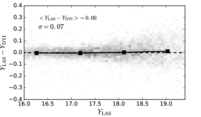
Figure 4: Photometric calibration accuracy of $Y$-band data versus UKIDSS LAS data. The grey points represent stars cross-matched with SDSS standard star catalog in Stripe 82 field with signal-to-noise ratio larger than 10 in both $Y$ bands. The mean differences in given magnitude bins, shown as black squares, are stable and close to zero.

4 Multi-band Photometry

At mentioned above, the VVDS-F22 field has also been covered by various surveys, such as SDSS, CFHTLS, UKIDSS LAS & DXS, and NVSS, from optical to radio. To construct our multi-band photometry catalog in the DYI field, we opt to incorporate the CFHTLenS data in optical (Heymans et al., 2012; Erben et al., 2013) and the UKIDS DXS data in near-infrared (Lawrence et al., 2007) in this field, respectively, as they are the deepest. Our catalog is based on our own photometry in these nine bands: $u^{*}$, $g^{\prime}$, $r^{\prime}$, $i^{\prime}$, $z^{\prime}$ (CFHTLenS); $Y$ (DYI); and $J$, $H$, $K$ (DXS). Table 2 summarizes the basic characteristics of these data. We note that the $H$-band data only cover $\sim$ 39% of the DYI field. We discuss our photometry in detail below.

Table 2: Summary of Multi-Band Data.

Band	FWHM[$\arcsec$]	Zeropoint	5$\sigma$ Depth	Survey
$u^{*}$	0.72-1.03	25.16	25.08	CFHTLenS
$g^{\prime}$	0.67-0.84	26.37	25.49	CFHTLenS
$r^{\prime}$	0.61-0.73	25.96	25.33	CFHTLenS
$i^{\prime}$	0.53-0.71	25.65	24.59	CFHTLenS
$z^{\prime}$	0.48-0.79	24.73	23.28	CFHTLenS
$Y$	0.56-1.33	24.30	22.86	CFHT DYI
$J$	0.69-1.10	25.45	23.51	UKIDSS DXS
$H$	0.64-1.08	26.10	23.15	UKIDSS DXS
$K$	0.55-1.32	25.94	23.20	UKIDSS DXS

4.1 Image Alignment and PSF Homogenization

When combining multi-band data for photometric redshift measurements, it is critical to carry out photometry homogeneously across all bands to obtain accurate color information. The most common treatment is to align all the images to the same grid and then perform the so-called “matched-aperture photometry , i.e., using the same aperture for a given object in all bands. We adopt this approach, and prepare our images as follows.

First, all the CFHTLenS and the DXS images are aligned to our $Y$-band images by using SWarp. In this process, the images are resampled to the pixel scale of 0.186″using Lanczos3 interpolation function, and projected to the tangential planes with maximum positional error of 0.001 pixel.

The next step is to homogenize the different PSF sizes among these images, which is necessary because the point-source FWHM values vary significantly among them. If this is not treated, using the same aperture for a given source in all bands would mean loosing different fraction of total light across the bands, which in turn would result in large systematic errors in the colors and consequently in photometric redshift measurements.

The most straightforward method of PSF homogenization is to degrade all the images to the PSF size of the image that has the worst point-source FWHM (e.g., Taylor et al. (2009); Cardamone et al. (2010)). The assumption is that the PSF of a given image is spatially invariant, which is a reasonable approximation in our case. For the sake of simplicity, we chose to degrade all images to the PSF size of the $Y$-band image that has the worst quality, which is the forth detector in tile F221+0330 with FHWM of 1.33″.

We constructed an empirical PSF for each image. To select the candidate PSF stars, we first run SExtractor to generate a catalog of bright sources, and retain only point-like sources based on the magnitude versus size diagram. This catalog is then matched to the SDSS Stripe 82 standard stars for refinement. To avoid any possible nonlinearity, we further restrict the peak pixel values of the selected stars to be less than half of the saturation level. The peak positions are then shifted to a common center by applying two dimensional cubic interpolation. We normalize the stars to their total fluxes, and perform median stack to construct the PSF for each image.

We use the IRAF task lucy, which is based on the Lucy-Richardson algorithm, to calculate the convolution kernels to convolve with the images. All images are then degraded to the PSF size of $1.33\arcsec$. Figure 5 shows the average curves of growth of the PSFs after homogenization for the nine band images. For comparison, the thick and thin dashed grey lines illustrate the curves of growth of the Gaussian and Moffat profiles with the same FWHM. Obviously, the empirical PSF is similar to Moffat profile, but more concentrated within radius of $1.8\arcsec$. We display the 2.2$\arcsec$ photometric aperture used for color and photometric redshift measurements as thick black line. For clarity, the inserted plot shows the corresponding ratios relative to the curve of growth with the largest PSF size. We can see that the residuals, resulting from the numerical approximation during the convolution, are less than 1.0% even at the very central region and close to zero at large radius. However, without the homogenization the maximum residual at the central region can reach to 25%.

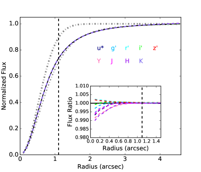
Figure 5: Average curves of growth of the nine bands after PSF homogenization. The black solid line shows the PSF with the worst seeing, while all the bands are displayed as color-coded dashed lines. The vertical dashed line is the 2.2$\arcsec$ photometric aperture for color measurements. The thick and thin dashed grey lines represent the Gaussian and Moffat functions with the same FWHM, respectively. The inserted figure shows the same curves of growth, but normalized to the worst one.

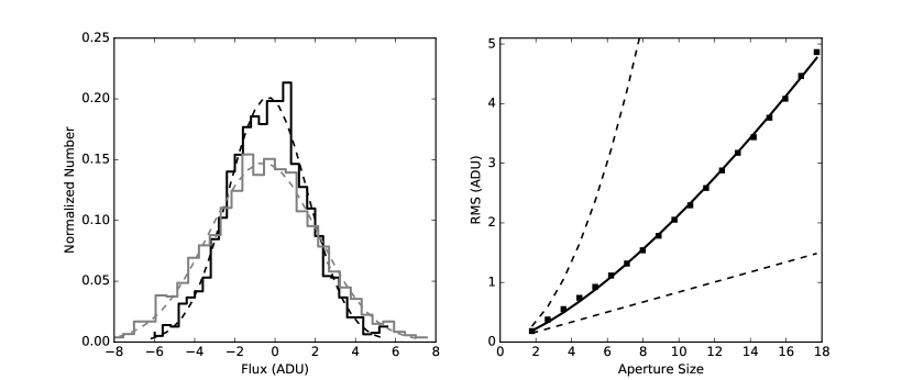
Figure 6: Left panel: histogram of number counts with aperture diameters of 2.0 and 2.5 arcsec. Their distributions have been normalized to unity. Larger aperture size shows more count variations and has larger Gaussian FWHM. Right panel: Gaussian rms curve in terms of aperture size defined as $\sqrt{N}$. Filled squares are measured directly from sky-subtracted image. A power-law function is used to fit the measurements. Meanwhile, the bottom and top dashed curves illustrate two limiting cases: no pixel correlation and complete correlation in adjacent pixels.

4.2 Source Detection and Photometry

For each band, the PSF matched images are stacked to one mosaic, which is about $2.1\times 1.1$ deg² in size. We then run SExtractor in dual-image mode for source detection and photometry. Due to the comparable depth to $Y$-band and good image quality, the non-PSF-homogenized $J$-band image is used as the detection image. The detection threshold is set to 1.5$\sigma$ above the background and at least three connected pixels are required for a measurement. In total, about 120,000 objects are detected in the multi-band images.

For each object we calculate two types of magnitudes, a specific aperture magnitude and the Kron-aperture magnitude (MAG_AUTO). In order to achieve an optimal signal-to-noise ratio estimate, generally, the aperture diameter is about 1.35$\times$FWHM if the point source has Gaussian PSF. However, from Figure 5 we know that the deviation between the empirical and Gaussian PSFs is very large. Therefore, the aperture diameter we use in this work for color and hence photometric redshift measurements is 2.2$\arcsec$ which is about 1.65 times of the FWHM. To remedy the missing fluxes due to the limited aperture, the aperture correction is applied based on the derived growth of curve. The Kron-aperture magnitude is measured within 2.5 times Kron radius (Kron, 1980) which accounts for over 96 per cent of the total flux of a galaxy, and provides an accurate estimate of the total magnitude.

We correct the Galactic extinction for the measured magnitudes using the dust maps from Schlegel et al. (1998) assuming R_V=3.1. The Galactic extinction curve is from Cardelli et al. (1989). The final corrections are less than 4.0% for optical bands and 1.0% for the near-infrared.

4.3 Noise Correction

There are two kinds of sources that contribute to photometric error budgets: photon shot noise from observed objects, and sky background fluctuations. The sky background noise can be, generally, determined by $\sigma^{2}=\sigma_{0}^{2}N$, where $\sigma_{0}$ is the standard deviation of background noise and $N$ is the pixel area for a given aperture. However, due to the existence of noise correlation stemming from resampling and PSF homogenization procedures, the standard formula will underestimate the photometric errors. Taking the noise correlation into account, the background noise estimate can be generalized as $\sigma^{2}\propto{N^{2\beta}}$ where $\beta$ is a free parameter within [0.5, 1.0]. In the case of pure background noise, $\beta=0.5$, which returns to the conventional formula. If the adjacent pixels are completely correlated, on the other hand, $\beta=1.0$.

We follow the recipe presented by Quadri et al. (2007) to determine $\beta$ for each image. Similar method can also be found in Gawiser et al. (2006) and Labbé et al. (2003). We randomly generate a set of $\sim$ 1000 positions on each band image which do not overlap with detected objects. The fluxes can be measured for each position using different apertures. For a given aperture, we fit the distribution of the measured fluxes with a Gaussian function. Larger aperture generally has larger Gaussian dispersion. Then we use the power-law equation described above to fit the relation between Gaussian dispersion and aperture size. While $\beta$ changes between different bands, the typical value is 0.6-0.8. Figure 6 shows an example of the fitting procedure for $Y$-band image. The correlated noise is transferred to the final magnitude errors by following the equation of error adopted by SExtractor.

5 Photometric Redshifts of Galaxies

We measure the photometric redshifts of the detected galaxies using the Bayesian photometric redshift code BPZ (Benítez, 2000; Coe et al., 2006). We also apply the EAZY code (Brammer et al., 2008) for comparison purposes. BPZ is a spectral template-based code in combination with a redshift prior derived from the spectroscopic redshifts in the Hubble Deep Field-North (HDF-N). EAZY is another template-fitting program which can linearly combine different templates and estimate realistic redshift uncertainties by introducing a novel rest-frame template error function. These two codes are constantly updated, and have been widely used in many studies. It should be noted that we are not aiming to compare the performance of the two codes themselves, but to study the characteristics of photometric redshifts derived by them. As in Hildebrandt et al. (2012), the recalibrated template set of Capak (2004) is used in this work. Before running the codes, we carry out two improvements as follows.

As discussed in Hildebrandt et al. (2012), since the peak of the posterior probability distribution, the product of the redshift likelihood and the Bayesian prior, is always at $z>0$, the photometric redshift values estimated by BPZ at low redshifts are systematically overestimated. Hildebrandt et al. (2012) modified the prior so that it no longer vanishes for z = 0. As a result, it leads to the improved photometric redshift estimate at low redshift. On the other hand, Raichoor et al. (2014) reconstructed the prior using SDSS spectroscopic Galaxy Main Sample (Strauss et al., 2002; Ahn et al., 2014) for galaxies with $12.5\,\mathrm{mag}\leq i^{\prime}\leq 17.0\,\mathrm{mag}$ and VVDS spectroscopic sample (Le Fèvre et al., 2013) for galaxies with $i^{\prime}\geq 20.0\,\mathrm{mag}$. For intermediate magnitudes, they interpolated the parameters of the prior to match those fitted at $i^{\prime}=17.0\,\mathrm{mag}$ and $i^{\prime}=20.0\,\mathrm{mag}$. The new prior can significantly reduce the photometric redshift bias and outliers for galaxies brighter than $20.0\,\mathrm{mag}$. Therefore, it improves the photometric redshift accuracy at low redshift ($z<0.4$). Here we also apply this new prior derived by Raichoor et al. (2014) to BPZ for photometric redshift measurements. As for EAZY, we use its default prior which is constructed with the synthetic photometry of galaxies in the semianalytic model (De Lucia & Blaizot, 2007). Unlike BPZ, one major feature of EAZY prior is that it does not impose any color restrictions as a function of redshift.

Any small color offsets of a few percent between different bands can affect the photometric redshift accuracy. For template-fitting methods, the commonly used strategy is to add some zeropoint offsets with an iterative process by comparing the measured and predicted colors (e.g. Ilbert et al. (2006); Cardamone et al. (2010); Hildebrandt et al. (2012)). By analyzing CFHTLenS data, Hildebrandt et al. (2012) concluded that such correction can suppress the PSF effects. Nevertheless, a proper PSF homogenization can be equivalent to the offset calibration if an accurate absolute photometric calibration is also performed. Our catalog, however, has two major differences compared to CFHTLenS data. First, it includes photometry from a number of surveys which span a period of many years and have different data reduction and calibration procedures. Secondly, we assume a constant PSF across a certain field without considering PSF variations. Therefore, it is essential to apply the offset calibration. We calculate the zeropoint offsets for different bands with the spectroscopic redshift sample described in Section 5.1 by fixing the redshifts to the spectroscopic values. For both codes, the derived absolute offset is about 0.11 mag for $J$ band, and less than 0.06 mag for any other band.

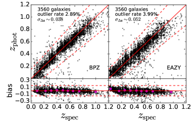
Figure 7: Top panel: comparison between the spectroscopic and photometric redshifts with $i^{\prime}$-band magnitude at $16.5\,\mathrm{mag}<i^{\prime}<24.0\,\mathrm{mag}$. The red dashed lines represent the outlier limit defined as $z_{\mathrm{p}}=z_{\mathrm{s}}\pm 0.15\times(1.0+z_{\mathrm{s}})$. Bottom panel: bias distribution as a function of spectroscopic redshifts. The magenta dots are the median values in eight redshift bins.

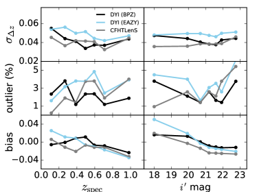
Figure 8: Photometric redshift statistics as a function of redshift (left) and $i^{\prime}$-band magnitude (right). Our results are shown as black (BPZ) and light blue (EAZY) lines, while CFHTLenS results are in grey. The magnitudes and redshifts are binned so that there are equal numbers of galaxies in each bin.

5.1 Photometric Redshift Accuracy

To check the accuracy of the photometric redshift measurements, we collect the spectroscopic redshifts of galaxies from three catalogs: the final data release of VVDS (Le Fèvre et al., 2013), the first data release of VIPERS (Garilli et al., 2014), and the SDSS DR12 spectra catalog (Alam et al., 2015). Among the catalogs, only galaxies with the most secure redshift measurements are selected. Specifically, galaxies with flag 3 and 4 (confidence level above 95%) are used for both VVDS and VIPERS data, while the SDSS galaxies are included to have spectra with zWarning equal to zero. For the duplicated galaxies the selection priority is VIPERS, VVDS and SDSS. In total, we obtain a sample of 3560 secure spectroscopic redshifts over the entire field. Their $i^{\prime}$-band magnitudes range from 16.5 to 24.0 mag, while the redshifts are in the range $0.02<z<1.5$ with median of $z=0.5$. Their positions are shown in Figure 1 as blue crosses.

We access the photometric redshift accuracy by comparing to the full spectroscopic sample. Following other studies (e.g. Hildebrandt et al. (2012)), we define the bias as $\Delta{z}=\delta{z}/(1.0+z_{\mathrm{spec}})$, where $\delta{z}=z_{\mathrm{phot}}-z_{\mathrm{spec}}$. Galaxies with $|\Delta{z}|>0.15$ are deemed as outliers. The Gaussian standard deviation of the bias is calculated after rejecting the outliers. Figure 7 shows the comparison between spectroscopic and photometric redshifts from the two codes. Overall, they display an satisfactory correspondence over the entire redshift range. The percentage of the outliers is about $2.89\%$ and $3.99\%$ for BPZ and EAZY, respectively. The $\Delta{z}$ distribution without including outliers can be well fitted by a Gaussian function, and the derived dispersion is $\sigma_{\Delta{z}}\sim 0.038$ and $0.052$ for the two codes, respectively. For the photometric redshifts from EAZY, the scatters and the outlier rates are somewhat larger than those of BPZ. But the two results do not show systematic biases. We further perform the same statistics for CFHTLenS photometric redshifts, derived with BPZ, using the spectroscopic sample. Due to the existence of the large mask regions around saturated stars in CFHTLenS catalog, there are a total of 2962 cross-matched galaxies. As a result, the outlier rate and standard deviation are $2.40\%$ and $0.038$ for our photometric redshifts estimated with BPZ ($3.65\%$ and $0.051$ for EAZY), while these are $2.70\%$ and $0.039$ for CFHTLenS. Though the sigma values are almost identical, our photometric redshift measurements with BPZ exhibit a somewhat lower outlier rate.

We further analyze the photometric redshift accuracy as a function of spectroscopic redshift and $i^{\prime}$-band magnitude. Figure 8 shows how the standard deviation, outlier rate and bias depend on the two measured quantities. The redshifts and magnitudes are binned so that there are equal numbers of galaxies in each bin. For comparison, the statistics for CFHTLenS are illustrated as grey lines. For redshift below 0.4 and magnitude brighter than 20.0 mag, our photometric redshift measurements with BPZ exhibit relatively large $\sigma_{\Delta{z}}$ and outlier rate. However, the outlier rate shows better performance for galaxies at $z>0.4$ and faint magnitudes ($i^{\prime}\gtrsim 21.0$ mag). Furthermore, the bias is smaller than that of CFHTLenS almost over the entire redshift and magnitude ranges. Table 3 provides more detailed comparison in different spectroscopic redshift bins. The median value of the 95% confidence intervals in a given bin is calculated to characterize the statistical error of the Bayesian posterior probability. The BPZ ODDS parameter is another quantity to describe the unimodality of a galaxy’s posterior redshift distribution, and we show the fraction of galaxies with ODDS$\geq$0.9 in Table 3. Significant improvements of the photometric redshift accuracy can be seen by comparing the two catalogs. In summary, in the redshift range $0.0<z_{\mathrm{spec}}<1.5$ at $i^{\prime}\lesssim 24.0$ mag, the catastrophic fraction of our photometric redshifts estimated with BPZ is no more than 4.0%, and the scatter is in the range $0.03<\sigma_{\Delta{z}}<0.06$.

Figure 9 compares our photometric redshift results of galaxies with those of CFHTLenS. To ensure the comparison to be conclusive, we only use the photometric redshifts estimated with BPZ and restrict the galaxies to have ODDS values larger than 0.9 and SExtractor FLAGS=0 in both samples. With these criteria, most of the galaxies at redshift $z\gtrsim 1.3$ in CFHTLenS sample are rejected because of the large photometric redshift uncertainties. We split the $i^{\prime}$-band magnitudes into three bins: $i^{\prime}<22.0$ mag, $22.0\,\mathrm{mag}<i^{\prime}<23.0\,\mathrm{mag}$, and $23.0\,\mathrm{mag}<i^{\prime}<24.0\,\mathrm{mag}$. The number of galaxies in each bin is listed in the corresponding panels. The figure shows an sharp decrease for $z_{\mathrm{CFHTLenS}}$ at $z\sim 0.1$ for $i^{\prime}<23.0$ mag. As stated in (Hildebrandt et al., 2012), it is mainly attributed to the selected redshift prior. For $z\gtrsim 0.2$, our photometric redshift measurements show unbiased correspondence with $z_{\mathrm{CFHTLenS}}$ (scatter $\sim$ 0.039, outlier rate $\sim$ 3.82%). However, for fainter galaxies ($23.0\,\mathrm{mag}<i^{\prime}<24.0\,\mathrm{mag}$) at redshift $z>0.6$, the photometric redshift scatter and outlier rate quickly increase to 0.06 and 11.4%. Taking the results presented in Figure 8 into account, our photometric redshifts are expected to be more accurate at high redshift due to the inclusion of near-infrared bands.

Table 3: Photometric Redshift (Estimated with BPZ) Quality Versus Redshift.

$z_{\mathrm{spec}}$	$n_{z}$	$w_{95}$	odds$\geq$0.9	bias	outlier	scatter
DYI
$(0.0,+)$	2962	0.191	98.5%	-0.002	2.4%	0.038
$(0.0,0.2]$	378	0.192	96.8%	-0.007	1.9%	0.055
$(0.2,0.4]$	697	0.196	98.6%	0.000	3.0%	0.043
$(0.4,0.6]$	840	0.192	99.5%	0.010	2.1%	0.037
$(0.6,0.8]$	679	0.189	98.2%	-0.011	1.3%	0.037
$(0.8,1.0]$	312	0.187	99.0%	-0.021	1.3%	0.043
$(1.0,+)$	56	0.177	94.6%	-0.079	19.6%	0.042
Without $Y$ band
$(0.0,+)$	2962	0.190	98.6%	-0.007	2.4%	0.039
$(0.0,0.2]$	378	0.190	98.9%	-0.016	1.1%	0.052
$(0.2,0.4]$	697	0.194	98.6%	-0.008	3.2%	0.043
$(0.4,0.6]$	840	0.191	98.9%	0.007	2.3%	0.038
$(0.6,0.8]$	679	0.189	98.1%	-0.012	1.8%	0.038
$(0.8,1.0]$	312	0.186	99.0%	-0.024	1.3%	0.044
$(1.0,+)$	56	0.176	96.4%	-0.085	19.6%	0.044
CFHTLenS
$(0.0,+)$	2962	0.271	79.9%	-0.013	2.7%	0.039
$(0.0,0.2]$	378	0.262	89.9%	0.007	0.3%	0.045
$(0.2,0.4]$	697	0.293	61.1%	-0.015	1.3%	0.038
$(0.4,0.6]$	840	0.267	91.1%	-0.010	3.5%	0.044
$(0.6,0.8]$	679	0.267	83.8%	-0.012	2.7%	0.034
$(0.8,1.0]$	312	0.291	80.1%	-0.034	1.9%	0.043
$(1.0,+)$	56	0.419	30.4%	-0.077	30.4%	0.059

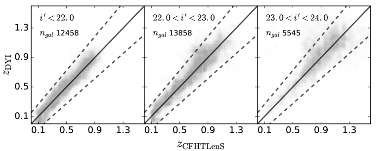
Figure 9: Comparison of the photometric redshifts measured by both our DYI (BPZ) and CFHTLenS in three $i^{\prime}$-band magnitude bins. The galaxies are selected to have ODDS$>$0.9 and SExtractor FLAGS=0 in both samples ($\sim$ 30,000 galaxies in total). The black dashed lines represent the outlier limit.

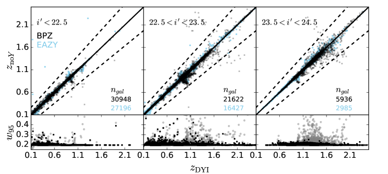
Figure 10: Top panel: comparison between the photometric redshifts without including $Y$ band ($z_{\mathrm{no}Y}$) and the photometric redshifts estimated by all bands with hight validation in three $i^{\prime}$-band magnitude bins. Total $\sim$ 59,000 galaxies for BPZ (black dots) and $\sim$ 47,000 for EAZY (light blue dots) are selected with ODDS$>$0.95 and reduced $\chi^{2}\leq 1.0$. The black dashed lines represent the outlier limit. Bottom panel: the 95% confidence interval as a function of redshift. Black dots indicate the photometric redshifts estimated with BPZ using all bands, while grey dots are $z_{\mathrm{no}Y}$.

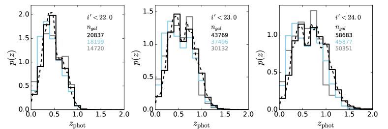
Figure 11: Redshift distributions for three magnitude limits: $i^{\prime}<22.0$ mag, $i^{\prime}<23.0$ mag, and $i^{\prime}<24.0$ mag. The black solid line and light blue line show the distributions of DYI photometric redshifts estimated with BPZ and EAZY, respectively, and the black dashed line is the stacking of corresponding posterior probabilities calculated with BPZ. For comparison, grey lines display the distributions of CFHTLenS photometric redshifts in the same field. The galaxies in the three samples are selected with reliable photometric redshift measurements (i.e. ODDS$>$0.9 and reduced $\chi^{2}\leq 1.0$). Their numbers in each magnitude bin are listed. Note that there are total $\sim$ 80,000 and $\sim$ 283,000 galaxies in DYI and CFHTLenS samples, respectively, before applying the selection criteria.

5.2 Photometric Redshifts Without $Y$ Band

One of our goals is to analyze the effect of the $Y$-band photometry on galaxy’s photometric redshift measurements. Because the dominant 4000 Å break feature of galaxies is redshifted to $Y$ band at redshift range $z\sim 1.25-1.8$, including $Y$ band should improve the photometric redshift estimate for that range. However, there are only very few spectroscopic redshifts larger than $z\sim 1.2$ in the field (see Table 3). To extend the redshift range, instead, we select a subsample of photometric redshifts estimated by all bands with high validation (ODDS$>$0.95 and reduced $\chi^{2}\leq 1.0$), and compare the photometric redshifts excluding the $Y$ band ($z_{\mathrm{no}Y}$) with this subsample, as shown in the top panel of Figure 10. For BPZ, we can see that they show good correspondence with scatter less than 0.008 at $z<1.0$ in the three magnitude bins. For $z$ in the range $1.0<z<2.0$, where the 4000 Å break basically locates in $Y$-band wavelength, $z_{\mathrm{no}Y}$ presents a large scatter of about 0.017 after rejecting outliers. Beyond $z\sim 2.0$, the scatter decreases again because the 4000 Å break has shifted to longer wavelengths. Similar results are also presented for photometric redshifts from EAZY.

In addition to degrading the photometric redshift accuracy, the exclusion of $Y$-band photometry would also reduce its precision. The bottom panel of Figure 10 presents the comparison of the 95% confidence interval, denoted as $w_{95}$, as a function of redshift. Due to the different definitions on the confidence level between the two photometric redshift codes, here we only show the results from BPZ, though we can draw a very similar conclusion from EAZY. The black dots in the figure indicate the photometric redshifts measured with all bands, while grey dots are $z_{\mathrm{no}Y}$. It is seen that the precision of $z_{\mathrm{no}Y}$ gets worse at $1.0<z<2.0$ as the galaxies become fainter. We arbitrarily define the fraction of $w_{95}>0.22$ to analyze the precision quantitively. For the three magnitude bins, the fraction increases from 0.2% to 10.4% for $z_{\mathrm{no}Y}$, while it is always less than 0.6% for $z_{\mathrm{DYI}}$. Based on the above analysis, we conclude that the inclusion of $Y$-band photometry can capture the 4000 Å break so that it is capable to improve the photometric redshift measurements at redshift range $1.0<z<2.0$.

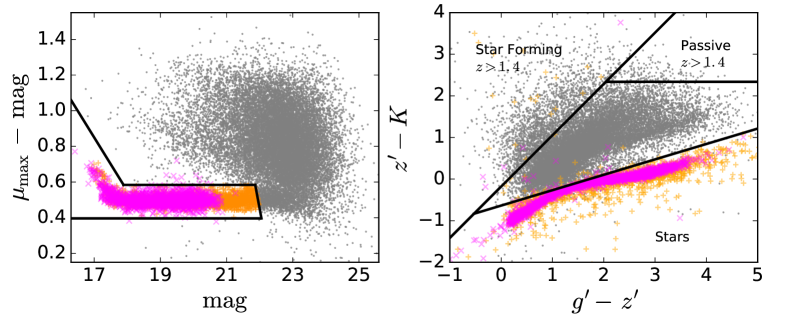
Figure 12: Left panel: separation between the point and extended sources within the $\mu_{\mathrm{max}}-\mathrm{mag}$ versus mag plane. The black line region indicates the locus of the point sources, shown as dark orange crosses ($+$). The two parallel lines are the $4\sigma$ limits of the locus. The SDSS photometric standard stars are overlaid as magenta crosses ($\times$). Right panel: star and galaxy distributions in the $g^{\prime}z^{\prime}K$ color-color diagram. The black lines represent the classification between stars and different $BzK$ galaxy populations (Daddi et al., 2004). Note that ($z^{\prime}-K$) has been adjusted by -0.163 mag to match the relation derived by Bielby et al. (2012) with WIRCam $K_{s}$ band. The distribution of our final selected stars are shown as orange crosses ($+$).

5.3 Redshift Distribution

We present the redshift distributions of the measured photometric redshifts at three $i^{\prime}$-band magnitude limits in Figure 11. The black solid lines and light blue lines display the distributions of the reliable photometric redshifts estimated with BPZ and EAZY, respectively, and the black dashed lines are the corresponding stacked posterior probabilities calculated with BPZ. They present good agreements in the given magnitude limits. For comparison, we also show the distributions of CFHTLenS photometric redshifts in the same field. As excepted, the galaxy fraction at $z>1.0$ is larger for our DYI photometric redshifts because of the more reliable measurements. We note that there are double peaks for magnitude limits $i^{\prime}<23.0$ mag and $i^{\prime}<24.0$ mag in the three photometric redshift distributions. Similar behavior also presents in several other studies (e.g. Ilbert et al. (2006); Coupon et al. (2009); Hildebrandt et al. (2012); Kuijken et al. (2015)). Hildebrandt et al. (2012) discussed that the multiple peaks probably result from the effects of filter set and selected redshift prior. In addition, Bonnett et al. (2016) analyzed the photometric redshifts of Dark Energy Survey Science Verification (DES SV) data using different photometric redshift codes. The resulted redshift distributions have different behaviors, displaying either multiple peaks or single peak. Therefore, the presence of multiple peaks is also likely to be model-dependent. Complete spectroscopic redshift sample down to $i^{\prime}\sim 24.0$ mag and detailed simulations are needed to address the question in detail.

5.4 Star-Galaxy Separation

We combine three criteria to separate stars from galaxies, the first using the maximum surface brightness ($\mu_{\mathrm{max}}$) versus magnitude diagram, the second using the $g^{\prime}z^{\prime}K$ color diagram (analog to the $BzK$ diagram presented by Daddi et al. (2004)), and the third comparing the reduced $\chi^{2}$ derived by galaxy and stellar spectral templates. We note that the similar method has also been discussed by Moutard et al. (2016).

The bright point sources can be well separated in the $\mu_{\mathrm{max}}$ versus magnitude diagram due to the proportional relation between the light distribution of the a point source and its magnitude (Leauthaud et al., 2007). We use $i^{\prime}$-band photometry for the selection, and cut the maximum surface brightness to a given limit $\mu^{lim}_{\mathrm{max}}$. The locus of the point sources are within the black line region as shown in the left panel of Figure 12. The selected point source sample by this criterion is denoted as $\mathbf{S_{1}}$.

The $BzK$ diagram was first proposed by Daddi et al. (2004) to select moderate redshift ($z\gtrsim$ 1.4) star-forming and passive galaxies. But it also turns out to be efficient for star and galaxy separation. Bielby et al. (2012) transformed the equations of $BzK$ selection into $g^{\prime}z^{\prime}K_{s}$ color-color plane, where $g^{\prime}z^{\prime}$ are CFHT MegaPrime filters and $K_{s}$ CFHT WIRCam filter. Because the $K$ filter we are using is from UKIRT WFCam, an offset of -0.163 mag is corrected for our ($z^{\prime}-K$) color with the new conversion constant between the Vega and AB magnitude of WIRCam $K_{s}$ filter (Muñoz et al., 2014). The right panel of Figure 12 displays the distribution of all objects in the $g^{\prime}z^{\prime}K$ diagram. The SDSS Stripe 82 photometric standard stars, shown as magenta crosses ($\times$), are also overlaid for illustration. The stars are obviously separated from galaxies by the solid black line $(z^{\prime}-K)<0.37\times(g^{\prime}-z^{\prime})-0.637$. The stars selected in the $g^{\prime}z^{\prime}K$ diagram is denoted as $\mathbf{S_{2}}$.

Lastly, we rerun BPZ on the catalog with the stellar spectral library from Pickles (1998) by fixing the redshift to zero. The zeropoint offsets are also adjusted to fit the stellar templates. Then the objects are flagged as stars if they satisfy $\chi^{2}_{\mathrm{star}}<2\times\chi^{2}_{\mathrm{gal}}$, where the factor 2 has been set because of the different degrees of freedom resulting from the use of independent galaxy and stellar templates (e.g. Hildebrandt et al. (2012)). We denote the stars satisfied this criterion as $\mathbf{S_{3}}$.

The stars are identified finally by combining the three criteria as follows:

• $\mathbf{S_{1}}\cap(\mathbf{S_{2}}\cup\mathbf{S_{3}})$, for $\mu_{\mathrm{max}}<\mu^{lim}_{\mathrm{max}}$;

• $\mathbf{S_{2}}\cap\mathbf{S_{3}}$, for $\mu_{\mathrm{max}}>\mu^{lim}_{\mathrm{max}}$.

In addition, for objects without available photometry in one of the $g^{\prime}z^{\prime}K$ bands, we only use the third criterion $\mathbf{S_{3}}$ for the classification. We select a subsample of 6236 unsaturated stars from SDSS standard star catalog, and confirm that only 0.5% stars are missed by our selection method. Finally, about 23.9% objects are classified as stars, and the fraction is similar to that of UKIDSS DXS catalog, which is $\sim$ 23.4%, in the same field.

5.5 Catalog

We compile our final photometric catalog in FITS table format. In the catalog, we include the geometric and photometric parameters calculated by SExtractor. Although several parameters (e.g. FLAGS, CLASS_STAR, FWHM_IMAGE, FLUX_RADUIS, MU_MAX, and SNR_WIN) are different between different bands, only these in $i^{\prime}$ band are adopted. Note that the aperture and total magnitudes are not corrected for Galactic extinction, while the extinctions are given in separate columns. The photometric redshifts are estimated only by the galaxy spectral templates without discriminating stars or galaxies so that the estimated redshifts of stars are not all to be zero. Therefore, the parameter “type” should be used for star and galaxy separation in practice. The detailed description on the catalog can be seen in Table 4.

Table 4: Table Contents of Our Multi-band Photometric Catalog.

Column NO.	Column Name	Describtion
1	id	Unique identification number, beginning from 1
2, 3	ra, dec	SExtractor right ascension and declination (J2000; decimal degrees)
4	type	Star and galaxy classification, star: type=1; galaxy: type=0
5	flag	SExtractor FLAGS
6	class_star	SExtractor CLASS_STAR
7	fwhm	SExtractor FWHM assuming a Gaussian profile (pixels)
8, 9	A_image, B_image	SExtractor profile rms along major and minor axes (pixel)
10	theta_image	SExtractor position angle (degree)
11	Kron_radius	SExtractor Kron aperture
12	flux_radius	SExtractor half-light radius (pixel)
13	mu_max	SExtractor peak surface brightness (mag/arcsec2)
14	snr	SExtractor signal-to-noise ratio SNR_WIN
15	zb	BPZ photometric redshift
16, 17	zb_min, zb_max	Lower and upper bound at 95% confidence level of zb
18	odds	BPZ ODDS parameter
19	chi2	BPZ reduced $\chi^{2}$
20	nfilt	Number of filters used in BPZ for measuring photometric redshifts
21-29	ext_$x$	Galactic extinction in the $x$ band (mag)
30-38	$x$mag	Magnitude in the $x$ band measured within 2.2″aperture diameter
39-47	$x$mag_err	Magnitude error in the $x$ band corrected for correlation noise
48-56	$x$magtot	Total magnitude in the $x$ band
57-65	$x$magtot_err	Total magnitude error in the $x$ band corrected for correlation noise

6 Summary

In this paper, we present a new deep CFHT WIRCam $Y$-band imaging covering about $2.0$ square degrees in VVDS-F22 field. Many efforts have been taken to properly handle various complications in image reduction and photometry. The final stack has reached 5$\sigma$ limit of 22.86 mag within a 2.2″  aperture for point sources. The photometric dispersion, compared to UKIDSS LAS $Y$-band data, is 0.07 mag. The final catalog includes broadband photometry from CFHTLenS optical images ($u^{*}g^{\prime}r^{\prime}i^{\prime}z^{\prime}$) and UKIDSS DXS images ($JHK$) after PSF homogenization, totaling $\sim$ 80,000 galaxies.

We derive photometric redshifts using both BPZ package with updated redshift priors and EAZY. Comparing with spectroscopic redshifts, we find that the catastrophic fraction of our photometric redshifts is no more than 4.0%, and the scatter is in the range $0.03<\sigma_{\Delta{z}}<0.06$. We also compare our photometric redshifts of galaxies with the corresponding CFHTLenS photometric redshifts derived by five optical bands in the same field. Although the two sets of results are based on different PSF homogenization strategies, they are generally consistent at $z>0.2$. For faint magnitude ($23.0\,\mathrm{mag}<i^{\prime}<24.0\,\mathrm{mag}$) at $z>0.6$, however, the outlier rate reaches to 11.4%. In that case, our photometric redshifts are expected to be more reliable thanks to the inclusion of near-infrared bands. It is also confirmed by comparing with the spectroscopic redshifts.

Many ongoing and upcoming wide field surveys, especially for weak lensing studies, include $Y$ band for accurate photometric redshift measurements beyond $z\sim 1.0$. We quantitatively analyze the impact of $Y$-band photometry on measuring photometric redshifts. Because there are very few spectroscopic redshifts at $z>1.2$ in the field, we select the most secure photometric redshifts measured by the full bands in the catalog as reference, and compare with the photometric redshifts without including $Y$-band photometry. For $1.0<z<2.0$, the $Y$-excluded photometric redshifts present large scatter due to the inaccurate identification of the 4000 Å break. Our analyses verify that $Y$-band photometry can improve both the accuracy and the precision of photometric redshift measurements at $z\sim 1.0-2.0$.

Our multi-band data, including images, photometry catalog and photometric redshifts, are available at the website: http://astro.pku.edu.cn/astro/data/DYI.html.

References

- Ahn et al. (2014) Ahn, C. P., Alexandroff, R., Allende Prieto, C., et al. 2014, ApJS, 211, 17
- Alam et al. (2015) Alam, S., Albareti, F. D., Allende Prieto, C., et al. 2015, ApJS, 219, 12
- Annis et al. (2014) Annis, J., Soares-Santos, M., Strauss, M. A., et al. 2014, ApJ, 794, 120
- Benítez (2000) Benítez, N. 2000, ApJ, 536, 571
- Bertin & Arnouts (1996) Bertin, E., & Arnouts, S. 1996, A&AS, 117, 393
- Bertin et al. (2002) Bertin, E., Mellier, Y., Radovich, M., et al. 2002, Astronomical Data Analysis Software and Systems XI, 281, 228
- Bertin (2006) Bertin, E. 2006, Astronomical Data Analysis Software and Systems XV, 351, 112
- Bielby et al. (2012) Bielby, R., Hudelot, P., McCracken, H. J., et al. 2012, A&A, 545, A23
- Bonnett et al. (2016) Bonnett, C., Troxel, M. A., Hartley, W., et al. 2016, Phys. Rev. D, 94, 042005
- Brammer et al. (2008) Brammer, G. B., van Dokkum, P. G., & Coppi, P. 2008, ApJ, 686, 1503-1513
- Buton et al. (2013) Buton, C., Copin, Y., Aldering, G., et al. 2013, A&A, 549, A8
- Cardamone et al. (2010) Cardamone, C. N., van Dokkum, P. G., Urry, C. M., et al. 2010, ApJS, 189, 270
- Capak (2004) Capak, P. L. 2004, Ph.D. Thesis, 3497
- Cardelli et al. (1989) Cardelli, J. A., Clayton, G. C., & Mathis, J. S. 1989, ApJ, 345, 245
- Coe et al. (2006) Coe, D., Benítez, N., Sánchez, S. F., et al. 2006, AJ, 132, 926
- Condon et al. (1998) Condon, J. J., Cotton, W. D., Greisen, E. W., et al. 1998, AJ, 115, 1693
- Coupon et al. (2009) Coupon, J., Ilbert, O., Kilbinger, M., et al. 2009, A&A, 500, 981
- Cross et al. (2012) Cross, N. J. G., Collins, R. S., Mann, R. G., et al. 2012, A&A, 548, A119
- Daddi et al. (2004) Daddi, E., Cimatti, A., Renzini, A., et al. 2004, ApJ, 617, 746
- De Lucia & Blaizot (2007) De Lucia, G., & Blaizot, J. 2007, MNRAS, 375, 2
- Dye et al. (2006) Dye, S., Warren, S. J., Hambly, N. C., et al. 2006, MNRAS, 372, 1227
- Erben et al. (2013) Erben, T., Hildebrandt, H., Miller, L., et al. 2013, MNRAS, 433, 2545
- Garilli et al. (2008) Garilli, B., Le Fèvre, O., Guzzo, L., et al. 2008, A&A, 486, 683
- Garilli et al. (2014) Garilli, B., Guzzo, L., Scodeggio, M., et al. 2014, A&A, 562, A23
- Hewett et al. (2006) Hewett, P. C., Warren, S. J., Leggett, S. K., & Hodgkin, S. T. 2006, MNRAS, 367, 454
- Heymans et al. (2012) Heymans, C., Van Waerbeke, L., Miller, L., et al. 2012, MNRAS, 427, 146
- High et al. (2010) High, F. W., Stubbs, C. W., Stalder, B., Gilmore, D. K., & Tonry, J. L. 2010, PASP, 122, 722
- Hildebrandt et al. (2012) Hildebrandt, H., Erben, T., Kuijken, K., et al. 2012, MNRAS, 421, 2355
- Ilbert et al. (2006) Ilbert, O., Arnouts, S., McCracken, H. J., et al. 2006, A&A, 457, 841
- Ilbert et al. (2009) Ilbert, O., Capak, P., Salvato, M., et al. 2009, ApJ, 690, 1236
- Ivezić et al. (2007) Ivezić, Ž., Smith, J. A., Miknaitis, G., et al. 2007, AJ, 134, 973
- Gawiser et al. (2006) Gawiser, E., van Dokkum, P. G., Herrera, D., et al. 2006, ApJS, 162, 1
- Kron (1980) Kron, R. G. 1980, ApJS, 43, 305
- Kuijken et al. (2015) Kuijken, K., Heymans, C., Hildebrandt, H., et al. 2015, MNRAS, 454, 3500
- Labbé et al. (2003) Labbé, I., Franx, M., Rudnick, G., et al. 2003, AJ, 125, 1107
- Laigle et al. (2016) Laigle, C., McCracken, H. J., Ilbert, O., et al. 2016, ApJS, 224, 24
- Laureijs et al. (2011) Laureijs, R., Amiaux, J., Arduini, S., et al. 2011, arXiv:1110.3193
- Lawrence et al. (2007) Lawrence, A., Warren, S. J., Almaini, O., et al. 2007, MNRAS, 379, 1599
- Leauthaud et al. (2007) Leauthaud, A., Massey, R., Kneib, J.-P., et al. 2007, ApJS, 172, 219
- Le Fèvre et al. (2013) Le Fèvre, O., Cassata, P., Cucciati, O., et al. 2013, A&A, 559, A14
- LSST Science Collaboration et al. (2009) LSST Science Collaboration, Abell, P. A., Allison, J., et al. 2009, arXiv:0912.0201
- Maddox et al. (2008) Maddox, N., Hewett, P. C., Warren, S. J., & Croom, S. M. 2008, MNRAS, 386, 1605
- Moutard et al. (2016) Moutard, T., Arnouts, S., Ilbert, O., et al. 2016, A&A, 590, A102
- Muñoz et al. (2014) Muñoz, R. P., Puzia, T. H., Lançon, A., et al. 2014, ApJS, 210, 4
- Pickles (1998) Pickles, A. J. 1998, PASP, 110, 863
- Puget et al. (2004) Puget, P., Stadler, E., Doyon, R., et al. 2004, Proc. SPIE, 5492, 978
- Quadri et al. (2007) Quadri, R., Marchesini, D., van Dokkum, P., et al. 2007, AJ, 134, 1103
- Raichoor et al. (2014) Raichoor, A., Mei, S., Erben, T., et al. 2014, ApJ, 797, 102
- Ramsay et al. (1992) Ramsay, S. K., Mountain, C. M., & Geballe, T. R. 1992, MNRAS, 259, 751
- Richards et al. (2002) Richards, G. T., Fan, X., Newberg, H. J., et al. 2002, AJ, 123, 2945
- Sánchez et al. (2014) Sánchez, C., Carrasco Kind, M., Lin, H., et al. 2014, MNRAS, 445, 1482
- Schlegel et al. (1998) Schlegel, D. J., Finkbeiner, D. P., & Davis, M. 1998, ApJ, 500, 525
- Skrutskie et al. (2006) Skrutskie, M. F., Cutri, R. M., Stiening, R., et al. 2006, AJ, 131, 1163
- Strauss et al. (2002) Strauss, M. A., Weinberg, D. H., Lupton, R. H., et al. 2002, AJ, 124, 1810
- Taylor et al. (2009) Taylor, E. N., Franx, M., van Dokkum, P. G., et al. 2009, ApJS, 183, 295
- van Dokkum (2001) van Dokkum, P. G. 2001, PASP, 113, 1420
- Warren et al. (2000) Warren, S. J., Hewett, P. C., & Foltz, C. B. 2000, MNRAS, 312, 827
- Wu & Jia (2010) Wu, X.-B., & Jia, Z. 2010, MNRAS, 406, 1583
- York et al. (2000) York, D. G., Adelman, J., Anderson, J. E., Jr., et al. 2000, AJ, 120, 1579