Learning to superoptimize programs

Abstract

Superoptimization requires the estimation of the best program for a given computational task. In order to deal with large programs, superoptimization techniques perform a stochastic search. This involves proposing a modification of the current program, which is accepted or rejected based on the improvement achieved. The state of the art method uses uniform proposal distributions, which fails to exploit the problem structure to the fullest. To alleviate this deficiency, we learn a proposal distribution over possible modifications using Reinforcement Learning. We provide convincing results on the superoptimization of “Hacker’s Delight” programs.

1 Introduction

Superoptimization requires us to obtain the optimal program for a computational task. While modern compilers implement a large set of rewrite rules, they fail to offer any guarantee of optimality. An alternative approach is to search over the space of all possible programs that are equivalent to the compiler output, and select the one that is the most efficient. If the search is carried out in a brute-force manner, we are guaranteed to achieve superoptimization. However, this approach quickly becomes computationally infeasible as the number of instructions and the length of the program grows.

To address this issue, recent approaches have started to use a stochastic search procedure, inspired by Markov Chain Monte Carlo sampling [15]. One of the main factors that governs the efficiency of this stochastic search is the choice of a proposal distribution. Surprisingly, the state of the art method, Stoke [15] relies on uniform distributions for each of its components. We argue that this choice fails to fully exploit the power of stochastic search.

To alleviate the aforementioned deficiency of Stoke, we build a reinforcement learning framework to estimate a more suitable proposal distribution for the task at hand. The quality of the distribution is measured as the expected quality of the program obtained via stochastic search. Using training data, which consists of a set of input programs, the parameters are learnt via the REINFORCE algorithm [18]. We demonstrate the efficacy of our approach on a set of “Hacker’s Delight” [17] programs. Preliminary results indicate that a learnt proposal distribution outperforms the uniform one on novel tasks that were previously unseen during training.

2 Related Works

The earliest approached for superoptimization relied on brute-force search. By sequentially enumerating all programs in increasing length orders [5, 12], the shortest program meeting the specification is guaranteed to be found. As expected, this approach scales poorly to longer programs or to large instruction sets. The longest reported synthesized program was 12 instructions long, on a restricted instruction set [12].

Trading off completeness for efficiency, stochastic methods [15] reduced the number of programs to test by guiding the exploration of the space, using the observed quality of programs encountered as hints. However, using a generic, unspecific exploratory policy made the optimization blind to the problem at hand. We propose to tackle this problem by learning the proposal distribution.

Similar work was done to discover efficient implementation of computation of value of degree $k$ polynomials [19]. Programs were generated from a grammar, using a learned policy to prioritize exploration. This particular approach of guided search looks promising to us, and is in spirit similar to our proposal, although applied on a very restricted case.

Another approach to guide the exploration of the space of programs was to make use of the gradients of differentiable relaxation of programs. Bunel et al. [2] attempted this by simulating program execution using recurrent Neural Networks. This however provided no guarantee that the optimum found was going to correspond to a real program. Additionally, this method only had the possibility of performing very local moves, limiting the kind of discoverable transformations.

Outside of program optimization, applying learning algorithms to improve optimization procedures, either in terms of results achieved or time taken, is a well studied subject. Doppa et al. [4] proposed methods to deal with structured output spaces, in a “Learning to search” framework. However, these approaches based on Imitation Learning are not directly applicable as we have access to a valid cost function, and therefore don’t need to learn how to approximate it. More relevant is the recent literature on learning to optimize. Li and Malik [11] and Andrychowicz et al. [1] learns how to improve on first-order gradient descent algorithms, making use of neural networks. Our work is similar, as we aim to improve the optimization process. We differ in that our initial algorithm is a MCMC sampler, on a discrete space, as opposed to gradient descent on a continuous, unconstrained space.

The training of a Neural Network to generate a proposal distribution to be used in sequential Monte-Carlo was also proposed by Paige and Wood [14] as a way to accelerate inference in graphical models. Additionally, similar approaches were successfully employed in computer vision problems where data driven proposals allowed to make inference feasible [8, 10, 20].

3 Learning Stochastic Superoptimization

Stoke performs black-box optimization of a cost function on the space of programs, represented as a series of instructions. Each instruction is composed of an opcode, specifying what to execute, and some operands, specifying the corresponding registers. Each given input program $\mathcal{T}$ defines a cost function. For a candidate program $\mathcal{R}$ called a rewrite, the associated cost is given by:

$$\textnormal{cost}\left(\mathcal{R},\mathcal{T}\right)=\omega_{e}\times\textnormal{eq}(\mathcal{R},\mathcal{T})+\omega_{p}\times\textnormal{perf}(\mathcal{R})$$ (1)

The term $\textnormal{eq}(\mathcal{R};\mathcal{T})$ measures how well do the outputs of the rewrite match with the outputs of the reference program when executed. This can be obtained either by running a symbolic validator or by running test cases, and accepting partial definition of correctness. The other term, $\textnormal{perf}(\mathcal{R})$ is a measure of the execution time of the program. An approximation can be the sum of the latency of all the instructions in the program. Alternatively, timing the program on some test cases can be used.

To find the optimum of this cost function, Stoke runs an MCMC sampler, using the Metropolis algorithm. This allows to sample from the probability distribution induced by the the cost function:

$$p(\mathcal{R};\mathcal{T})=\frac{1}{Z}\exp(-\textnormal{cost}\left(\mathcal{R},\mathcal{T}\right))),$$ (2)

where $\mathcal{R}$ is the proposed rewrite, $\mathcal{T}$ is the input program.

The sampling is done by proposing random moves $\mathcal{R}\rightarrow\mathcal{R}^{\star}$, sampled from a proposal distribution $q(\mathcal{R^{\star}}|\mathcal{R})$. An acceptance criterion is computed, and used as the parameter of a Bernoulli distribution, to decide whether or not the move is accepted.

$$\alpha(\mathcal{R}\rightarrow\mathcal{R}^{\star},\mathcal{T})=\min\left(1,\frac{p(\mathcal{R^{\star};\mathcal{T}})}{p(\mathcal{R;\mathcal{T}})}\right).$$ (3)

The proposal distribution $q$ originally used in [15] is a hierarchical model, whose detailed structure distribution can be found in Appendix A. Uniform distributions were used for each of the elementary probability distributions the model sample from. This corresponds to a specific instantiation of the general approach. We propose to learn those probability distribution so as to maximize the probability of reaching the best programs.

The cost function defined in equation (1) corresponds to what we want to optimize. Under a fixed computational budget to perform program superoptimization in less than $T$ iterations, we are interested in having the lowest possible cost at the end. As different programs have different runtimes and therefore different associated costs, we need to perform normalization. As normalized loss function, we use the ratio between the best rewrite found and the cost of the initial unoptimized program $\mathcal{R}_{0}$. Given that our optimization procedure is stochastic, we will need to consider the expected cost as our loss. This expected loss is a function of the parameters $\theta$ of our proposal distribution. The objective function of our “meta-optimization” problem is therefore:

$$\mathcal{L}(\theta)=\mathbb{E}_{\{\mathcal{R}_{t}\}\sim q_{\theta}}\left[\frac{\min_{t=0..T}\textnormal{cost}\left(\mathcal{R}_{t},\mathcal{T}\right)}{\textnormal{cost}\left(\mathcal{R}_{0},\mathcal{T}\right)}\right]$$ (4)

Our chosen parameterization of $q$ is to keep the hierarchical structure of the original work of Schkufza et al. [15], and parameterize all separate probability distributions (over the type of move, the opcodes, the operands, and the lines of the program) independently. In order to learn them, we will make use of unbiased estimators of the gradient. These can be obtained using the REINFORCE algorithm [18]. A helpful way to derive them is to consider the execution traces of the search procedure under the formalism of stochastic computation graphs [16]. The corresponding graph used can be found in Appendix B.

By instrumenting the Stoke system of Schkufza et al. [15], we can collect the execution traces so as to compute gradients over the outputs of the probability distributions, which can then be back-propagated. In that way, we can perform Stochastic Gradient Descent (SGD) over our objective function 4.

4 Experiments

We ran our experiments on the Hacker’s delight [17] corpus, a collection of 25 bit-manipulation programs, used as benchmark in program synthesis [7, 9, 15]. A detailed description of the task is given in Appendix C. Some examples include identifying whether an integer is a power of two from its binary representation, counting the number of bits turned on in a register or computing the maximum of two integers.

In order to have a larger corpus than the twenty-five programs initially obtained, we generate various starting points for each optimization. This is accomplished by running Stoke with a cost function where $\omega_{p}=0$ in (1), keeping only the correct programs and filtering out duplicates. This allows us to create a larger dataset.

We divide the Hacker’s Delight tasks into two sets. We train on the first set and only evaluate performance on the second so as to evaluate the generalization of our learned proposal distribution. We didn’t attempt to learn the probability distribution over the operands and the program position, only learning the ones over opcodes and type of move to perform.

The probability distribution learned here are simple categorical distribution. We learn the parameters of each separate distribution jointly, using a Softmax transformation to enforce that they are proper probability distribution. We initialize the training with uniform proposal distribution so the first datapoints on the graph corresponds to the original system of  [15].

In our current experiment, the proposal distributions are not conditioned on the input program. Optimizing them corresponds to finding an ideal proposal distribution for Stoke. Figure 1(a) shows the results. Both the training and the test loss decreases and it can be observed that the optimization of program happens faster and that more programs reach the observed minimum.

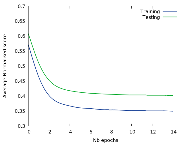
(a) Evolution of the Objective function.

Model Training Test Uniform 57.38% 60.90 % Learned Bias 34.93 % 40.16%

(b) Final improvement score on the Hacker’s Delight benchmark.

Figure 1: Initializing from Uniform Distributions as in Stoke [15], we manage to improve performance by learning the proposal distribution.

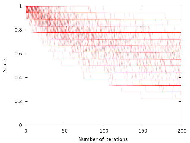
(a) Optimization Traces

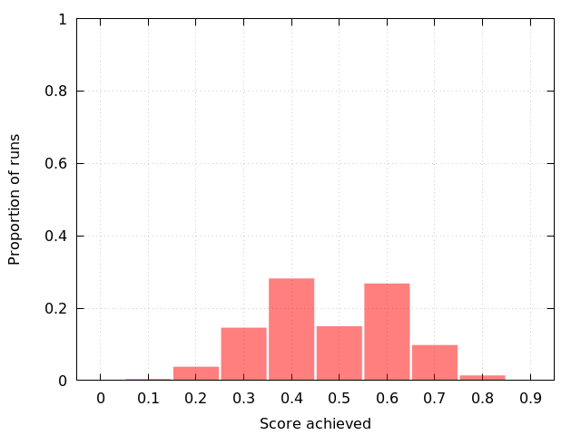
(b) Scores after 200 iterations

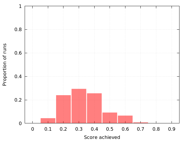
(c) Scores after 400 iterations

Figure 2: Optimization Results using Uniform elementary distributions

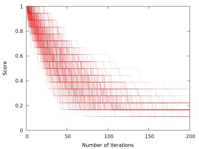
(a) Optimization Traces

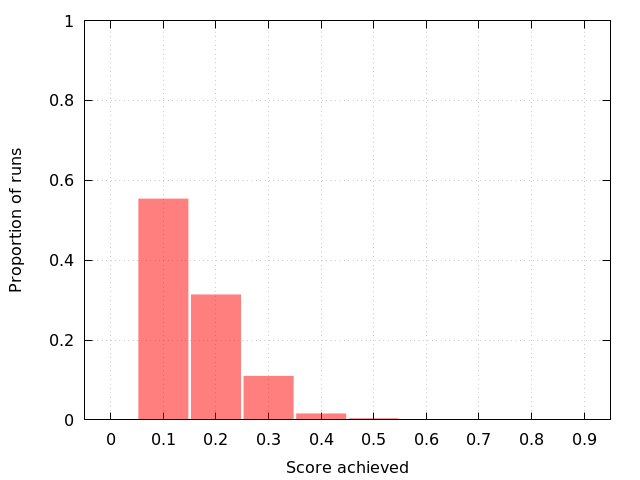
(b) Scores after 100 iterations

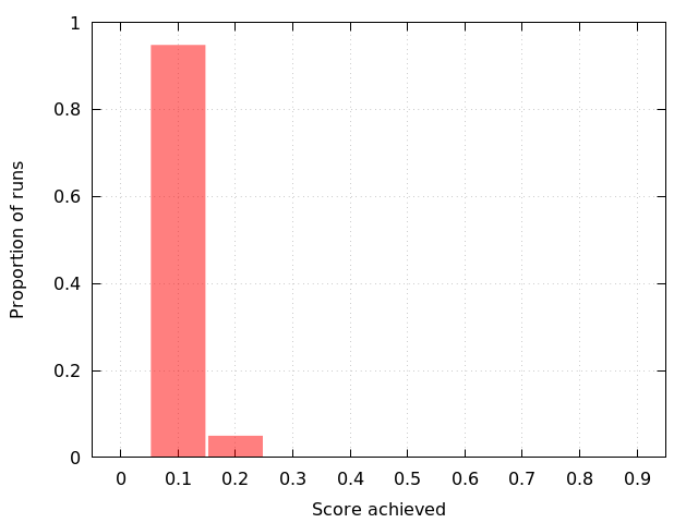
(c) Scores after 200 iterations

Figure 3: Optimization Results using Learned elementary distributions. Even with less iterations, better results are achieved than when using Uniform distributions.

5 Conclusion

Within this paper, we have shown that learning the proposal distribution of the stochastic search can lead to significant performance improvement. It is interesting to compare our approach to the synthesis-style approaches that have been appearing recently in the Deep Learning community [6] that aim at learning programs directly using differentiable representations of programs. We note one advantage that such stochastic search-based approach yields is that the resulting program can be run independently from the Neural Network that was used to discover them.

Several improvements are possible to the presented approach. Making the probability distribution a Neural Network conditioned on the initial input or on the current state of the rewrite would lead to a more expressive model, while essentially having similar training complexity. It will however be necessary to have a richer, more varied dataset to make any evaluation meaningful.

Appendix A Generative model of the program transformations

In Stoke [15], the program transformation are sampled from a generative model. This process was analysed from the publicly available code [3].

First, a type of transformation is sampled uniformly from the following proposals method.

1. Add a NOP instruction Add an empty instruction at a random position in the program.

2. Delete an instruction Remove one of the instruction of the program.

3. Instruction Transform Replace one existing line (instruction + operands) by a new one (New instruction and new operands).

4. Opcode Transform Replace one instruction by another one, keeping the same operands. The new instruction is sampled from the set of compatible instructions.

5. Opcode Width Transform Replace one instruction by another one, with the same memonic. This means that those instructions do the same thing, except that they don’t operate on the same part of the registers (for example, will replace movq that move 64-bit of data of the registers by movl that will move 32-bit of data)

6. Operand Transform Replace the operand of a randomly selected instruction by another valid operand for the context, sampled at random.

7. Local swap Transform Swap two instructions in the same “block”.

8. Global Swap transform Swap any two instructions.

9. Rotate transform Draw two positions in the program, and rotate all the instructions between the two (the last one becomes the first one of the series and all the others get pushed back).

Then, once the type of move has been sampled, the actual move has to be sampled. To do that, a certain numbers of sampling steps need to happen. Let’s take as example 3.

To perform an Instruction Transform,

1. A line in the existing programs is uniformly chosen.

2. A new instruction is sampled, from the list of all possible instructions.

3. For each of the arguments of the instruction, sample from the acceptable value.

4. The chosen line is replaced by the new line that was sampled.

The sampling process of a move is therefore a hierarchy of sampling steps. A simple way to characterize it is as a generative model over the moves. Depending on what type of move is sampled, differents series of sampling steps will have to be performed. For a given move, all the probabilities are sampled independently so the probability of proposing the move is the product of the probability of picking each of the sampling steps. The generative model is defined in Figure 4. It is going to be parameterized by the the parameters of each specific probability distribution it samples from. The default Stoke version uses uniform probabilities over all of those elementary distributions.

⬇ 1def proposal(current_program): 2 move_type = sample(categorical(all_move_type)) 3 if move_type == 1: % Add empty Instruction 4 pos = sample(categorical(all_positions(current_program))) 5 return (ADD_NOP, pos) 6 7 if move_type == 2: % Delete an Instruction 8 pos = sample(categorical(all_positions(current_program))) 9 return (DELETE, pos) 10 11 if move_type == 3: % Instruction Transform 12 pos = sample(categorical(all_positions(current_program))) 13 instr = sample(categorical(set_of_all_instructions)) 14 arity = nb_args(instr) 15 for i = 1, arity: 16 possible_args = possible_arguments(instr, i) 17 % get one of the arguments that can be used as i-th 18 % argument for the instruction ’instr’. 19 operands[i] = sample(categorical(possible_args)) 20 return (TRANSFORM, pos, instr, operands) 21 22 if move_type == 4: % Opcode Transform 23 pos = sample(categorical(all_positions(current_program))) 24 args = arguments_at(current_program, pos) 25 instr = sample(categorical(possible_instruction(args))) 26 % get an instruction compatible with the arguments 27 % that are in the program at line pos. 28 return(OPCODE_TRANSFORM, pos, instr) 29 30 if move_type == 5: % Opcode Width Transform 31 pos = sample(categorical(all_positions(current_program)) 32 curr_instr = instruction_at(current_program, pos) 33 instr = sample(categorical(same_memonic_instr(curr_instr)) 34 % get one instruction with the same memonic that the 35 % instruction ’curr_instr’. 36 return (OPCODE_TRANSFORM, pos, instr) 37 38 if move_type == 6: % Operand transform 39 pos = sample(categorical(all_positions(current-program)) 40 curr_instr = instruction_at(current_program, pos) 41 arg_to_mod = sample(categorical(args(curr_instr))) 42 possible_args = possible_arguments(curr_instr, arg_to_mod) 43 new_operand = sample(categorical(possible_args)) 44 return (OPERAND_TRANSFORM, pos, arg_to_mod, new_operand) 45 46 if move_type == 7: % Local swap transform 47 block_idx = sample(categorical(all_blocks(current_program))) 48 possible_pos = pos_in_block(current_program, block_idx) 49 pos_1 = sample(categorical(possible_pos)) 50 pos_2 = sample(categorical(possible_pos)) 51 return (SWAP, pos_1, pos_2) 52 53 if move_type == 8: % Global swap transform 54 pos_1 = sample(categorical(all_positions(current_program))) 55 pos_2 = sample(categorical(all_positions(current_program))) 56 return (SWAP, pos_1, pos_2) 57 58 if move_type == 9: % Rotate transform 59 pos_1 = sample(categorical(all_positions(current_program))) 60 pos_2 = sample(categorical(all_positions(current_program))) 61 return (ROTATE, pos_1, pos_2)

Figure 4: Generative Model of a Transformation

The criterion described in equation (3) is justified at the condition that the proposal distribution is symmetric, that is, $q(\mathcal{R}^{\star}|\mathcal{R})=q(\mathcal{R}|\mathcal{R}^{\star})$. In that case, in the limit, the distribution of states visited by the sampler will be $p$, making the optimal program the most sampled [13].

By learning the proposal distribution, we won’t necessarily maintain the symmetry property. Even when using only uniform elementary distributions as in [15], the proposal distribution is not symmetric. An example showing the non-symmetric characteristic is the case of the Instruction Transform move.

If the proposal is to replace an instruction with two arguments by one with one argument, the probability of the proposal will be:

$$q(\mathcal{R}^{\star}|\mathcal{R})=\frac{1}{n_{\textnormal{moves}}}\times\frac{1}{n_{\textnormal{opcodes}}}\times\frac{1}{n_{\textnormal{operands}}},$$ (5)

while the reverse proposal would be:

$$q(\mathcal{R}|\mathcal{R}^{\star})=\frac{1}{n_{\textnormal{moves}}}\times\frac{1}{n_{\textnormal{opcodes}}}\times\frac{1}{n^{2}_{\textnormal{operands}}},$$ (6)

As a consequence, the proposal distribution is not symmetric and the properties of the Metropolis algorithm [13] won’t apply. Even without guarantees in the limit, the whole process can still be understood as an hill-climbing algorithm with a stochastic component to avoid getting stuck in local maxima.

Another potential solution would be to use the Metropolis-Hastings criterion to replace the simpler Metropolis criterion (3):

$$\alpha(\mathcal{R}\rightarrow\mathcal{R}^{\star},\mathcal{T})=\min\left(1,\frac{p(\mathcal{R^{\star};\mathcal{T}})q(\mathcal{R}|\mathcal{R^{\star}})}{p(\mathcal{R;\mathcal{T}})q(\mathcal{R^{\star}}|\mathcal{R})}\right).$$ (7)

However, this involves developping an inverse model of the proposed moves to find for each move, the reverse move that would correspond to its undoing and estimate their probabilities. In the current form of the proposal distribution in Figure 4, not all moves have a direct reverse move. For example, Delete does not.

Appendix B Metropolis algorithm as a Stochastic Computation Graph

Figure 5: Stochastic Computation Graph of the Metropolis algorithm used for program superoptimization. Round nodes are stochastic nodes and square ones are deterministic. Red arrows corresponds to computation done in the forward pass that needs to be learned while green arrows correspond to the backward pass. Full arrow represent deterministic computation and dashed arrow represent stochastic ones. The different steps of the forward pass are:
(1) Based on features of the reference program, the proposal distribution $q$ is computed.
(2) A random move is sampled from the probability distribution and we keep track of the probability of taking this move.
(3) The score of the rewrite that would be obtained by applying the chosen move is measured experimentally.
(4) The acceptance criterion for the move is computed.
(5) The move is accepted with a probability equal to the acceptance criterion.
(6) Move 2-7 are repeated $N$ times.
(7) The reward is observed, corresponding to the best program obtained during the search.

Appendix C Hacker’s delight tasks

The 25 tasks of the Hacker’s delight [17] datasets are the following:

1. Turn off right-most one bit

2. Test whether an unsigned integer is of the form $2^{(}n-1)$

3. Isolate the right-most one bit

4. Form a mask that identifies right-most one bit and trailing zeros

5. Right propagate right-most one bit

6. Turn on the right-most zero bit in a word

7. Isolate the right-most zero bit

8. Form a mask that identifies trailing zeros

9. Absolute value function

10. Test if the number of leading zeros of two words are the same

11. Test if the number of leading zeros of a word is strictly less than of another work

12. Test if the number of leading zeros of a word is less than of another work

13. Sign Function

14. Floor of average of two integers without overflowing

15. Ceil of average of two integers without overflowing

16. Compute max of two integers

17. Turn off the right-most contiguous string of one bits

18. Determine if an integer is a power of two

19. Exchanging two fields of the same integer according to some input

20. Next higher unsigned number with same number of one bits

21. Cycling through 3 values

22. Compute parity

23. Counting number of bits

24. Round up to next highest power of two

25. Compute higher order half of product of x and y

References

- Andrychowicz et al. [2016] Marcin Andrychowicz, Misha Denil, Sergio Gomez, Matthew W Hoffman, David Pfau, Tom Schaul, and Nando de Freitas. Learning to learn by gradient descent by gradient descent. In NIPS, 2016.
- Bunel et al. [2016] Rudy Bunel, Alban Desmaison, Pushmeet Kohli, Philip HS Torr, and M Pawan Kumar. Adaptive neural compilation. In NIPS. 2016.
- Churchll et al. [2016] Berkeley Churchll, Eric Schkufza, and Stefan Heule. Stoke. https://github.com/StanfordPL/stoke, 2016.
- Doppa et al. [2014] Janardhan Rao Doppa, Alan Fern, and Prasad Tadepalli. Hc-search: A learning framework for search-based structured prediction. JAIR, 2014.
- Granlund and Kenner [1992] Torbjörn Granlund and Richard Kenner. Eliminating branches using a superoptimizer and the GNU C compiler. ACM SIGPLAN Notices, 1992.
- Graves et al. [2014] Alex Graves, Greg Wayne, and Ivo Danihelka. Neural turing machines. CoRR, 2014.
- Gulwani et al. [2011] Sumit Gulwani, Susmit Jha, Ashish Tiwari, and Ramarathnam Venkatesan. Synthesis of loop-free programs. In PLDI, 2011.
- Jampani et al. [2015] Varun Jampani, Sebastian Nowozin, Matthew Loper, and Peter V Gehler. The informed sampler: A discriminative approach to bayesian inference in generative computer vision models. Computer Vision and Image Understanding, 2015.
- Jha et al. [2010] Susmit Jha, Sumit Gulwani, Sanjit A Seshia, and Ashish Tiwari. Oracle-guided component-based program synthesis. In International Conference on Software Engineering, 2010.
- Kulkarni et al. [2015] Tejas D Kulkarni, Pushmeet Kohli, Joshua B Tenenbaum, and Vikash Mansinghka. Picture: A probabilistic programming language for scene perception. In CVPR, 2015.
- Li and Malik [2016] Ke Li and Jitendra Malik. Learning to optimize. CoRR, 2016.
- Massalin [1987] Henry Massalin. Superoptimizer: A look at the smallest program. In ACM SIGPLAN Notices, 1987.
- Metropolis et al. [1953] Nicholas Metropolis, Arianna W Rosenbluth, Marshall N Rosenbluth, Augusta H Teller, and Edward Teller. Equation of state calculations by fast computing machines. The journal of chemical physics, 1953.
- Paige and Wood [2016] Brookes Paige and Frank Wood. Inference networks for sequential Monte Carlo in graphical models. In ICML, 2016.
- Schkufza et al. [2013] Eric Schkufza, Rahul Sharma, and Alex Aiken. Stochastic superoptimization. SIGPLAN, 2013.
- Schulman et al. [2015] John Schulman, Nicolas Heess, Theophane Weber, and Pieter Abbeel. Gradient estimation using stochastic computation graphs. In NIPS, 2015.
- Warren [2002] Henry S Warren. Hacker’s delight. 2002.
- Williams [1992] Ronald J Williams. Simple statistical gradient-following algorithms for connectionist reinforcement learning. Machine learning, 1992.
- Zaremba et al. [2014] Wojciech Zaremba, Karol Kurach, and Rob Fergus. Learning to discover efficient mathematical identities. In NIPS. 2014.
- Zhu et al. [2000] Song-Chun Zhu, Rong Zhang, and Zhuowen Tu. Integrating bottom-up/top-down for object recognition by data driven markov chain monte carlo. In CVPR, 2000.