Acceleration in Non-planar Time-dependent Billiard

Abstract

We study the dynamical properties of a particle in a non-planar square billiard. The plane of the billiard has a sinusoidal shape. We consider both the static and time-dependent plane. We study the affect of different parameters that control the geometry of the billiard in this model. We consider variations of different parameters of the model and describe how the particle trajectory is affected by these parameters. We also investigate the dynamical behavior of the system in the static condition using its reduced phase plot and show that the dynamics of the particle inside the billiard may be regular, mixed or chaotic. Finally, the problem of the particle energy growth is studied in the billiard with the time-dependent plane. We show that when in the static case, the billiard is chaotic, then the particle energy in the time-dependent billiard grows for small number of collisions, and then it starts to saturate. But when the dynamics of the static case is regular, then the particle average energy in the time-dependent situation stays constant.

I Introduction

Billiard is a dynamical system of a mass point particle which moves along geodesic lines inside a closed region. When the particle reaches the boundary, it would reflect elastically.

Despite the simplicity, billiard has a rich physics Robnik (1983), which makes it a powerful tool for modeling a vast range of physical phenomena and systems, from microwave field in resonators Richter (1999) to semiconductors Micolich (2000), optics Milner et al. (2001); Kaplan et al. (2005) and acoustic Kawabe et al. (2003).

The dynamics of a billiard is governed by the shape of the boundary and the geometry of the plane. The static non-planar billiards have been studied before and it was shown that although the square flat billiard is integrable, the non-planar square billiard can exhibit chaos Salazar and Téllez (2012). Until recently, only billiards with static curved plane has been studied. Here we investigate the billiard with time-dependent non-planar surface.

In the time-dependent situation, the particle may accelerate. This behavior that particles could be accelerated by time-dependent perturbations of the boundary, is known as Fermi acceleration. In Fermi (1949) Fermi explained the origin of heavy ion acceleration of cosmic rays. Fermi showed that, a classical particle may gain unbounded energy upon collisions with a heavy and moving wall. This is of particular interest, especially for understanding the unbounded ( indeterminate) energy growth in systems that a particle experiences collisions with a time-dependent boundary. Many billiards with time-dependent boundary as a two dimensional model of such systems have been studied Leonel et al. (2009); Loskutov and Ryabov (2002); Oliveira and Leonel (2010a); de Carvalho et al. (2006); Gelfreich et al. (2011). Attempts to explain the relation between exhibition of the Fermi acceleration in a time-dependent billiard and the nonlinear dynamics of its static version leaded to the Loskutov-Ryabov-Akinshin (LRA) conjecture. The LRA conjecture states that the “chaotic dynamics of a billiard with a fixed boundary is a sufficient condition for the Fermi acceleration in the system when a boundary perturbation is introduced” Loskutov et al. (2000). It was cleared that the existence of orbits of unbounded and rapid energy growth is a general phenomenon, typical for arbitrary slow non-autonomous perturbation of a Hamiltonian system with chaotic behavior Gelfreich and Turaev (2008a). It was also discussed in Gelfreich and Turaev (2008b) that another mechanism can accelerates the particle to unbounded energy. This showed that the presence of unbounded energy growth is possible for billiards which the phase space of their frozen case retains the small horseshoe for all times. The unbounded energy growth also can be observed in systems with zero Lyapanov exponentShah et al. (2010).

The quest for observation of unbounded energy growth and verifying the validity of the LRA conjecture are two of the motivations for studying time-dependent billiards in the recent decade Gelfreich et al. (2011); de Carvalho et al. (2006); Leonel et al. (2004); Leonel and Bunimovich (2010); Livorati et al. (2008); Oliveira and Leonel (2010a, b); Oliveira and Robnik (2012); Batistić (2014). The Fermi acceleration has been mostly studied in planar billiards with time-dependent boundary. However, energy growth due to the time-dependence of the plane of a billiard has not been studied yet. Here we investigate this problem and show that time-dependence of the curvature of the plane of a billiard may lead to some growth in average energy at first and then the average energy starts to saturate.

These studies could have potential applications in variety of phenomenon and fields, e.g., for understanding the dynamics of an electron confined in a curved graphene sheet or a crystal lattice. The graphene can be deformed to form a curved thin sheet. This thin layer of graphene can be considered as a plane of a non-planar billiard. This thin layer has some vibrations which makes its curvature time-dependent. For some applications like sensitive mass detection and high precision metrology, it is crucial to take these vibrations into account Dai et al. (2012). Since, the random shaped vibrations of graphene sheets can be expanded in terms of sinusoidal functions, the time-dependent sinusoidal shaped geometry is one of the ways to study this system.

Another application of our work is for cold atoms in optical traps where a cold atom is confined to a node of a standing wave with large wave length, thus the atom is approximately restricted to move on a flat two dimensional space Milner et al. (2001); Kaplan et al. (2005).

The applications of the investigation of particle behavior in a bounded time-dependent space can also be extended to general relativity. Recently, experiments are performed which emulates the general relativity phenomenon, like the study of the behavior of light in a curved space. This includes the study and simulation of the behavior of light, wave packets or solitons in a curved space Schultheiss et al. (2010); Bekenstein et al. (2014, 2015); Peschel and Trompeter (2007). These studies open a new horizon in understanding the general relativity and behaviors of celestial objects and probably new aspects of this theory.

Here, we study the dynamics of a particle in a rectangular non-planar billiard, where the plane of the billiard changes as a traveling sinusoidal wave. When, either of the amplitude or the wave vector of the surface vanishes, the system would be the well known flat rectangular billiard. Although the planar rectangular billiard is quiet integrable, we show that the static case, can be chaotic. In fact, the rectangle is chosen as the boundary, to show the transition from integrable to chaotic dynamics in the static situation. This generalizes previous studies in two aspects. First, we consider a particle in a non-planar billiard with time-dependent plane curvature. Second, we study the behavior of the energy growth of a particle in a time-dependent non-planar billiard.

The outline of our paper is as follows. In section II the theory and the numerical method are described. In section III the behavior of the particle is explored numerically. In the Sec. III A, we explain the effect of parameters of the system on the shape of a trajectory of the particle. In the Sec. III B, the dynamics of the particle in the static situation is discussed using the phase space Poincare section (where the static situation refers to when the wave velocity is zero). In Sec. III C. we investigate the behavior of the energy growth of the particle and the application of LRA conjecture to our model.

Finally, the section IV is the conclusion.

II Theory

In this model, a classical particle is constrained to move on a two dimensional time-dependent surface which is confined to a contour. This surface is embedded in the three-dimensional Euclidean space.

The surface $\varSigma$ is defined as

$$\varSigma:y^{i}=y^{i}\left(u^{1},u^{2};t\right)\mbox{ $$$$$$$$$\mbox{ $$$$$$}$},\mbox{ $$$$$$$$}i=1,2,3,$$ (1)

where $y^{i}$’s are Cartesian coordinates in the flat three-dimensional space and $u{}^{1},\,u^{2}$ are coordinates defined on the two-dimensional curved surface. The selection of $u{}^{1},\,u^{2}$ depends on surface symmetries.

The position of the particle constrained to the $\Sigma$, can be expressed as

$$\overset{\rightarrow}{r} = \overset{\rightarrow}{r}\left(u^{1},u^{2};t\right)=y^{1}\left(u^{1},u^{2};t\right)\hat{i}$$ (2)

$$+ y^{2}\left(u^{1},u^{2};t\right)\hat{j}+y^{3}\left(u^{1},u^{2};t\right)\hat{k}.$$

The motion of a particle which is constrained to the surface $\Sigma$ will depend on the surface geometry which is specified by the metric

$$a_{\alpha\beta}=\frac{\text{$\partial$}y^{i}(u^{1},u^{2};t)}{\text{$\partial$}u^{\alpha}}\frac{\text{$\partial$}y^{i}(u^{1},u^{2};t)}{\text{$\partial$}u^{\beta}}\mbox{ $$$$$$$$}\alpha\mbox{,}\beta=1,2.$$ (3)

The Lagrangian of a particle of mass $\mu$ with a potential $V\left(\overrightarrow{r}\right)$ constrained to the surface $\Sigma$ is

$$L=\frac{\mu}{2}a_{\alpha\beta}(u^{1},u^{2};t)\dot{u}^{\alpha}\dot{u}^{\beta}-V\left(\overrightarrow{r}\right)\mbox{ $$$$$$$$$\mbox{ $$$$$$$$}$},\mbox{ $$$$$$$$}\alpha\mbox{,}\beta=1,2,$$ (4)

For simplicity, we consider $V\left(\overrightarrow{r}\right)=0$ and $\mu=1$ in our model.

Using the Eq. 4, canonical momentums and the Euler-Lagrange equations are

$$p_{\alpha}=\text{$\partial$}_{\dot{u}^{\alpha}}L(u^{1},u^{2};t) = a_{\alpha\beta}(u^{1},u^{2};t)\dot{u}^{\beta},$$ (5)

$$\frac{d}{dt}\left(\frac{\text{$\partial$}L(u^{1},u^{2};t)}{\text{$\partial$}\dot{u}^{\alpha}}\right) - \frac{\text{$\partial$}L(u^{1},u^{2};t)}{\text{$\partial$}u^{\alpha}}=0.$$ (6)

In our model, we consider the motion of a particle on a traveling wave surface with a square boundary which, may be aligned in a direction other than the wave vector. The surface $\Sigma$ is defined as

$$\left\{\begin{array}[]{c}u^{1}=x\\ u^{2}=y\end{array}\right.\Longrightarrow\left\{\begin{array}[]{c}y^{1}=u^{1}\\ y^{2}=u^{2}\\ y^{3}=f\left(u^{1},u^{2};t\right)=\\ A\sin\left(k_{x}x+k_{y}y-\omega t\right)\end{array}\right.,$$ (7)

where $A$ and $\omega$ are the amplitude and angular frequency. The $k_{x}$ and $k_{y}$ are components of the wave vector, $k$.

$$k_{x} = k\cos\left(\theta_{wave}\right),$$

$$k_{y} = k\sin\left(\theta_{wave}\right).$$ (8)

where $k$ and $\theta_{wave}$ are respectively the magnitude of the wave vector and the angle between the wave vector, $\overrightarrow{k}$, and the $x$ axis. The magnitude of the wave velocity is specified by $V_{wave}=\frac{\omega}{k}$.

In this paper, we use "wave" to refer to the geometry of the surface.

Figure 1 gives four snapshots of the motion of the particle on the time dependent surface. In this figure, the wave fronts are aligned along the $y$ axis.

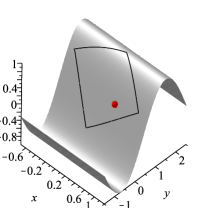
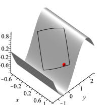
(a)

(b)

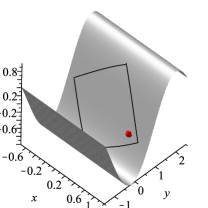
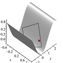
(c)

(d)

Figure 1: Illustration of four snapshots of a typical non-planar time-dependent billiard as explained in Eq. 7. Solid black lines show the boundary.

The metric for the surface in Eq. 7 is

$$\begin{array}[]{cc}a_{xx}=1+A^{2}k_{x}^{2}&a_{xy}=A^{2}k_{x}k_{y}\\ \cos^{2}\left(k_{x}x+k_{y}y-\omega t\right)&\cos^{2}\left(k_{x}x+k_{y}y-\omega t\right)\\ \\ a_{yx}=A^{2}k_{x}k_{y}&a_{yy}=1+A^{2}k_{y}^{2}\\ \cos^{2}\left(k_{x}x+k_{y}y-\omega t\right)&\cos^{2}\left(k_{x}x+k_{y}y-\omega t\right)\end{array}.$$ (9)

By considering that $k$ and $A$ are both real, this metric is a Riemannian metric. This is because the determinant of the metric is positive definite, i.e.,

$$a_{xx}a_{yy}-\left(a_{xy}\right)^{2}=1+A^{2}k^{2}\cos^{2}\left(k_{x}x+k_{y}y-\omega t\right)>0.$$

For the Lagrangian and the canonical momentums we get

$$L = \frac{1}{2}(a_{xx}(x,y;t)\dot{x}^{2}+2a_{xy}(x,y;t)\dot{y}\dot{x}$$ (10)

$$+ a_{yy}(x,y;t)\dot{y}^{2}),$$

$$p_{x} = \left(a_{xx}(x,y;t)\dot{x}+a_{xy}(x,y;t)\dot{y}\right),$$

$$p_{y} = \left(a_{yy}(x,y;t)\dot{y}+a_{yx}(x,y;t)\dot{x}\right).$$ (11)

Therefore, the equations of motion are the following (for more details see the Appendix)

$$\frac{d}{dt}(\frac{\text{$\partial$}}{\text{$\partial$}\dot{x}}(\frac{1}{2}(a_{xx}(x,y;t)\dot{x}^{2}+2a_{xy}(x,y;t)\dot{y}\dot{x}$$

$$+a_{yy}(x,y;t)\dot{y}^{2})))-\frac{\text{$\partial$}}{\text{$\partial$}x}((\frac{1}{2}(a_{xx}(x,y;t)\dot{x}^{2}$$

$$+2a_{xy}(x,y;t)\dot{y}\dot{x}+a_{yy}(x,y;t)\dot{y}^{2})))=0,$$

$$\frac{d}{dt}(\frac{\text{$\partial$}}{\text{$\partial$}\dot{y}}(\frac{1}{2}(a_{xx}(x,y;t)\dot{x}^{2}+2a_{xy}(x,y;t)\dot{y}\dot{x}$$

$$+a_{yy}(x,y;t)\dot{y}^{2})))-\frac{\text{$\partial$}}{\text{$\partial$}y}(\frac{1}{2}(a_{xx}(x,y;t)\dot{x}^{2}$$

$$+2a_{xy}(x,y;t)\dot{y}\dot{x}+a_{yy}(x,y;t)\dot{y}^{2}))=0.$$ (12)

Next, we explain our numerical methods. We consider the motion of a particle constrained to a time-varying surface (Eq. 7) with a square boundary. The square boundary is placed along the x and y axes. The position of the particle is found by solving equations of motion numerically. Here, we assume that the boundary is fixed with respect to the time-dependent surface $\Sigma$. When, the particle collides with the boundary, the velocity vector would reflect with respect to the boundary and only the normal component of the velocity would reverse. New components of the velocity are considered as the initial conditions for the dynamics after the collision.

In the next section, we explore numerical results for the dynamics of the particle.

III Numerical results

III.1 Trajectory of a particle

In this subsection, given the Eq. 7 as the plane of the billiard, we investigate behaviors of the trajectory of the particle in our model. We consider $x_{0}=\frac{2}{3},$ $y_{0}=0,$ $V=1$ and $V_{x}=0.7986355099$ as initial conditions of the particle. The wave amplitude, $A$, and the wave vector, $k$, control the behavior of the trajectory. We display the trajectory in the three-dimensional Euclidean space. Figures 2 and 3 illustrate the trajectories and show how $A$ and $k$ would change the trajectory.

Figure 2 displays the effect of the wave amplitude as a control parameter. In Fig. 2, we take $A=0.01$, $A=0.05$, $A=0.1$ and $A=0.5$ respectively. Other parameters; including the magnitude of the wave vector, the wave velocity, the wave direction and the time step are

$$k=0.1,V_{wave}=1,\theta_{wave}=\frac{\pi}{5},\text{$\Delta$}t=\frac{1}{80}.$$

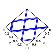
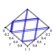
(a)

(b)

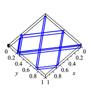
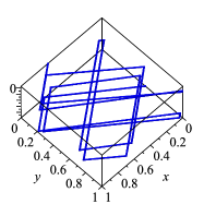
(c)

(d)

Figure 2: As $A$ increases, the trajectory of the particle becomes more irregular. We take $A=0.01$, $A=0.05$, $A=0.1$ and $A=0.5$ respectively.

As the amplitude of the wave increases, the billiard changes from the familiar flat square billiard to a non-planar square billiard. When, $A$ is small but non-zero, we see that the trajectory is close to the periodic orbit of the flat billiard (Fig. 2 (a)). As the amplitude of the wave increases, the shape of the trajectory becomes more irregular. In Fig. 2 (d) it becomes irregular.

Figure 3 displays the effect of increasing the magnitude of the wave vector. In Fig. 3, we take $k=0.01$, $k=0.1$, $k=1$ and $k=10$ respectively. Other parameters like the wave amplitude, the wave velocity magnitude, the wave direction and the time step are

$$A=0.15,V_{wave}=1,\theta_{wave}=\frac{\pi}{5},\text{$\Delta$}t=\frac{1}{80}.$$

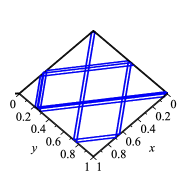
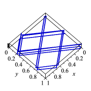
(a)

(b)

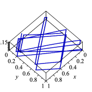
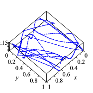
(c)

(d)

Figure 3: As $k$ increases, the trajectory of the particle becomes more irregular. We take $k=0.01$, $k=0.1$, $k=1$ and $k=10$ respectively.

The influence of the changes in the wave vector is similar to the changes in the wave amplitude. As the magnitude of the wave vector increases, the wave length would decreases. Then, the number of dips and peaks in the billiard region would increase at each instant of time. If the wave length is significantly greater than the dimensions of the billiard then the billiard is almost planar. Thus, as the wave length decreases, the trajectory of the point particle changes from the planar periodic orbit.

These diagrams illustrate that each of characteristics of the wave individually can influence the shape of trajectories. Therefore, it is hard to explain the behavior of a trajectory when all of these parameters have an effective role.

Furthermore, the direction of wave fronts with respect to the boundary of the billiard is also an important parameter. A typical example is the parallel case, when the wave vector is parallel with x or y axes, then the system has a symmetry plane. This symmetry plane is placed in the middle of the billiard and is parallel with the wave vector. But when the wave vector is along another direction, symmetries of the billiard would change. The net symmetry of the plane and the boundary of the billiard affects the motion of the particle. Preservation of symmetries determines the number of constants of motion and the number of independent constants of motion determines the dimensions of the subspace of the trajectory in the phase space. If there are N independent constants of motion, the motion is restricted to a subspace with dimension 4-N in phase space. (Notice that, when the system is not conservative, the energy is not a constant of motion. ). We will explain this in Sec. III. C.

III.2 Phase space

In this section, we study the dynamical behavior of the static case of this billiard. In this case, the wave velocity is zero. The wave velocity can be obtained by $\frac{\omega}{k}=V_{wave}$, thus, in the static case $\omega$ vanishes. Using the Eq. 7, the third component of the surface is obtained as $y^{3}=A\sin\left(k_{x}x+k_{y}y\right)$. Therefore, the billiard is a static sinusoidal surface with a square boundary. The Poincare section of the phase space of the static case is investigated in order to obtain its dynamical behavior. In Fig. 4, the trajectory of a particle in a typical static billiard is displayed.

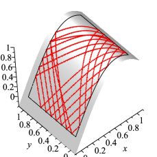
Figure 4: Illustration of the trajectory of a particle on a typical static billiard. The initial conditions are $x_{0}=1,y_{0}=\frac{1}{3},V_{x}=-.7193398005,V_{y}=0.6946583703$ and the other parameters used are $A=1,k=2,V_{wave}=0$ and $\theta_{wave}=0$.

The selection of variables of the reduced phase space is composed of arc length of each collision point $S\in\left[0,1\right]$ and the cosine of the angle between the incident velocity vector and the boundary. In Figs. 5 and 6 the reduced phase spaces are displayed for different static systems when the wave direction is $\frac{\pi}{5}$. We choose the amplitude of the wave and the magnitude of the wave vector as control parameters. Each reduced phase space is built using 30 initial conditions for the first 500 collisions with the boundary. Figure 5 shows how the wave amplitude affects the phase space diagram.

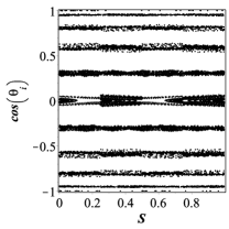
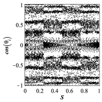
(a)

(b)

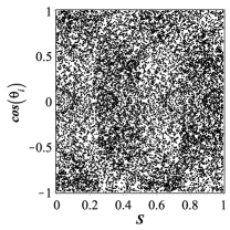
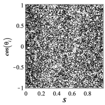
(c)

(d)

Figure 5: The reduced phase space illustrates that, by increasing the amplitude of the wave, the dynamics of the billiard becomes chaotic. The wave amplitude and wave vector used are (a) $k=1.5$ and $A=0.05$; (b) $k=1.5$ and $A=0.1$; (c) $k=1.5$ and $A=0.25$; and (d) $k=1.5$ and $A=1$.

A particle in non-planar billiard has two degree of freedom and hence, the phase space is four-dimensional. In the static situation, the energy is a constant of motion. In the planar billiard, the momentum is a constant of motion too. While in the non-planar case the symmetry of the billiard and as a consequence the momentum preservation break down. Figure 5 verifies this and shows that, the role of the growth of the wave amplitude in increasing the chaotic sea.

Next, the effect of increasing the magnitude of the wave vector (or decreasing the wave length) on the dynamics of the static system is shown in Fig. 6.

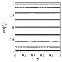
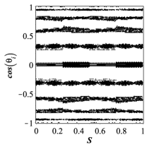
(a)

(b)

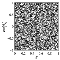
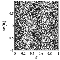
(c)

(d)

Figure 6: The reduced phase space illustrates that, by increasing the magnitude of the wave vector, the dynamics of the billiard becomes chaotic. The wave amplitude and wave vector used are (a) $k=0.01$ and $A=1$; (b) $k=0.1$ and $A=1$; (c) $k=0.5$ and $A=1$; and (d) $k=2$ and $A=1$.

It shows that, as the magnitude of the wave vector increases, stochastic points increase. This illustrates the transition of the dynamics of the billiard from integrable to chaotic.

As a result, by increasing the wave amplitude or the magnitude of the wave vector, the billiard deviates from the planar case. As the wave surface emerges in the interior of the square billiard, the symmetries of the billiard and the number of constants of motion changes. If the number of constants of motion decreases, then the dynamics of the billiard won’t be integrable anymore.

In following subsection, we show that in some cases more than one constant of motion exists.

III.3 Behavior of the energy growth

The main goal of this section is to show that two different behaviors of the particle energy growth are possible in this model. Furthermore, by considering their corresponding reduced phase plots, we study the application of the LRA conjecture for this model.

The LRA conjecture states that “chaotic dynamics of a billiard with a fixed boundary is a sufficient condition for the Fermi acceleration in the system when a boundary perturbation is introduced”. The perturbation as a time dependent change in the shape of a boundary has been investigated in Gelfreich et al. (2011); de Carvalho et al. (2006); Leonel et al. (2004); Leonel and Bunimovich (2010); Livorati et al. (2008); Oliveira and Leonel (2010a, b); Oliveira and Robnik (2012); Batistić (2014). Here, we extend these studies to a billiard with time-dependent plane. Thus, in this subsection the behavior of the average energy of the particle as a function of the number of collisions is studied for a time-dependent non-planar square billiard. Numerical investigations of the average energy behavior have been performed in two cases, when the energy grows and then converges to a constant value, and for a case that the energy remains approximately constant. The two cases are shown respectively in Figs. 7 and 10. Results are made in an ensemble of 30 particles for different initial conditions and characteristics of the wave. Here, we discuss our results in two separate cases.

Case 1. In Fig. 7, we consider a situation where the system exhibits limited energy growth and then it saturates.

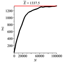
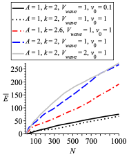
(a)

(b)

Figure 7: For $\theta_{wave}=\frac{\pi}{5}$, the average energy as a function of the number of collisions is calculated for an ensemble of 30 particles. (a) When the dynamics of the static case is chaotic, the average energy grows and then saturates. (b) For comparison, the behavior of energy growth for different values of the parameters of the system is simulated.

Figure 7 (a) shows that, the average energy increases for the small number of collisions, and then starts to saturate. The corresponding phase plot for this case is displayed in Fig. 6 (d). The phase plot shows that for this selection of the parameters, the system has a chaotic dynamics. Therefore, for the small number of collisions, the results in Fig. 7 are in agreement with the LRA conjecture. However, for sufficiently large number of iterations, our results don’t agree with the LRA conjecture and the average energy converges to the $\bar{E}=1337.5$.

We also compare the results for different values of parameters in Fig. 7 (b). An increase in either of the $k$, $V_{wave}$ or $A$ would result in increase of the particle energy.

In order to explain the behavior of the energy growth, we consider the particle on the wave without boundaries. The behavior of the energy of the free particle as a function of time (Fig. 8) explains why the energy grows and then saturates in Fig. 7 (a).

The behavior of the particle is better understood in a coordinate with diagonal metric. When the particle is in the billiard, we don’t use this coordinate system. By considering, $q^{1}=\frac{1}{k}\left(k_{x}x+k_{y}y\right)$, $q^{2}=\frac{1}{k}\left(-k_{y}x+k_{x}y\right)$, the metric would be diagonalized. By transforming the coordinates of the particle $\left(x,y\right)$ to the diagonal coordinates $\left(q^{1},q^{2}\right)$, we get

$$\begin{array}[]{c}\begin{array}[]{cc}a_{11}=1+A^{2}k^{2}\left(\cos\left(k\,q^{1}-\omega t\right)\right)^{2}&a_{12}=0\\ a_{21}=0&a_{22}=1\end{array},\\ \\ L=\frac{1}{2}\left(\left(1+A^{2}k^{2}\left(\cos\left(k\,q^{1}-\omega t\right)\right)^{2}\right)\left(\dot{q}^{1}\right)^{2}+\left(\dot{q}^{2}\right)^{2}\right),\\ \\ \frac{d}{dt}\frac{\partial L}{\partial\dot{q}^{1}}-\frac{\partial L}{\partial q^{1}}=0,\,\,\,\,\,\ddot{q}^{2}=0.\end{array}$$

The transformation equations show that, the first component of the diagonal coordinates is parallel, $v_{q^{1}}=\dot{q}^{1}$, and the other one is perpendicular to the wave vector, $v_{q^{2}}=\dot{q}^{2}$.

The equations of motion show that, the perpendicular component of the free particle velocity remains constant during the motion; while, the parallel component changes. Therefore, the behavior of the parallel component of the velocity is responsible for the energy evolution of the particle.

So, depending on the relative velocity of the particle and the wave, the energy may increase or decrease with respect to its initial value.

In Fig. 8, for all the plots, the initial velocity of the particle is in the direction of the wave vector. Only in one case the energy oscillates between the initial value and a lower value. While, in the other cases, the energy oscillates between its initial value and a higher value or remains constant.

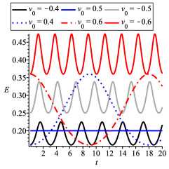
Figure 8: The time evolution of the free particle energy for different values of particle velocity when $\theta_{paricle}=\frac{\pi}{2},$ $\theta_{wave}=\frac{\pi}{2},$ $k=1,$ $A=1$ and $V_{wave}=0.5$.

Consequently, in most of these cases the energy grows. In non-integrable conditions, it is more probable that the particle collides with the boundary before its energy reaches its value at the previous reflection. In other words, it is more probable that the time interval between two successive collisions isn’t multiple of the period of energy evolution. Since, in most of the energy evolution, energy oscillates between its initial value and a higher value, it is more probable that the particle has a higher energy when it reaches the boundary. This is the reason of energy growth for the small number of collisions in Fig. 7. When, the particle velocity grows enough, the parallel component, $v_{q^{1}}$ is almost greater than the $V_{wave}$. There are two possible direction for $v_{q^{1}}$ and each of them would result in a different energy evolution. One of them oscillates between its initial value and a higher value of the energy and the other one oscillates between its initial value of the energy and a lower value. The balance of these two cases would result in the saturation behavior of the energy. These cases correspond to $v_{0}=0.6$ and $v_{0}=-0.6$ in Fig. 8.

In Fig. 9, we present the time evolution of the energy of a particle for one initial condition during successive impacts with the boundary in our model. The black crosses specify when the particle is reflected. As it is seen, the energy of the particle grows at the beginning of the motion.

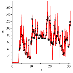
Figure 9: The time evolution of a particle energy with initial conditions $x_{0}=1,$ $y_{0}=\frac{1}{3},$ $V_{x}=-.7193398005$ and $V_{y}=0.6946583703$ in a system with $V_{wave}=1,$ $k=5,$ $A=1$ and $\theta_{wave}=\frac{\pi}{5}$.

Case 2. We now discuss the situation that, the particle average energy stays near a constant value.

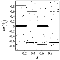
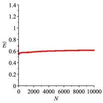
(a)

(b)

Figure 10: (a) The reduced phase plot of the static system of $k=1,$ $A=1$ and $\theta_{wave}=0$. (b) The behavior of the average energy for an ensemble of 30 particles as a function of the number of collisions in the corresponding time-dependent system. The average energy stays constant when the dynamics of the static case is integrable.

As shown in Fig. 10 (b), in contrast with the previous case, the average energy doesn’t grow. This figure shows that, even for the small iteration numbers, the average energy stays near a constant value which is approximately 0.68. The Fig. 10 (a) shows the phase plot of the corresponding static system.

In Fig. 10, the wave vector is parallel with two walls of the boundary. So, the system preserves a kind of symmetry. When the $\theta_{wave}=0$ , we find that the Eq. 7 has the following form

$$y^{1} = u^{1}=x,$$

$$y^{2} = u^{2}=y,$$

$$y^{3} = A\sin\left(k_{x}x-\omega t\right).$$

Thus, using the Eq. 9 the metric is diagonal

$$\begin{array}[]{cc}a_{xx}=1+A^{2}k_{x}^{2}\cos^{2}\left(k_{x}x-\omega t\right)&a_{xy}=0\\ a_{yx}=0&a_{yy}=1\end{array}.$$

Then, momentums and the Lagrangian are obtained as

$$p_{x} = \left(1+A^{2}k_{x}^{2}\cos^{2}\left(k_{x}x-\omega t\right)\right)\dot{x},$$

$$p_{y} = \dot{y},$$

$$L=\frac{1}{2}\left(\left(1+A^{2}k_{x}^{2}\cos^{2}\left(k_{x}x-\omega t\right)\right)\dot{x}^{2}+\dot{y}^{2}\right).$$

using the Lagrangian, equations of motion are written as

$$\frac{d}{dt}(\frac{\text{$\partial$}}{\text{$\partial$}\dot{x}}(\frac{1}{2}(a_{xx}(x,y;t)\dot{x}^{2}+\dot{y}^{2})))-$$

$$\frac{\text{$\partial$}}{\text{$\partial$}x}((\frac{1}{2}(a_{xx}(x,y;t)\dot{x}^{2}+\dot{y}^{2}))) = 0,$$

$$\frac{d}{dt}(\frac{\text{$\partial$}}{\text{$\partial$}\dot{y}}(\frac{1}{2}(a_{xx}(x,y;t)\dot{x}^{2}+\dot{y}^{2})))-$$

$$\frac{\text{$\partial$}}{\text{$\partial$}y}(\frac{1}{2}(a_{xx}(x,y;t)\dot{x}^{2}+\dot{y}^{2})) = 0.$$

This allows us to find the equation of motion for the y component as

$$\frac{d}{dt}\left(\dot{y}\right)=0.$$

Take into account that the $p_{y}=\dot{y}$, we find that the y component of the momentum is conserved. During the particle reflection from each wall of the square boundary, this component of the momentum would be the normal or the tangent component of the momentum and its value remains unchanged. Therefore, its conservation is preserved in the square billiard.

Moreover, considering $\omega=0$ in the static situation, it is easy to show that the $p_{y}$ is conserved in the static case, too. In addition, for the static case the energy is also conserved. So, the billiard in the static situation has two constants of motion. The phase plot of a static two dimensional billiard has a 4 dimensional phase space. When there are two constant of motion, the particle trajectory would be placed in a two dimensional subspace of the phase space. Therefore, the system which corresponds to the Fig. 10, is integrable. So, as mentioned before, the direction of the wave fronts with respect to the boundary plays an important role in preserving symmetries of the system.

The integrable dynamics implies no energy growth for the bouncing particle.

We expect that if the static version of this non-planar time-dependent billiard is integrable, then its energy wouldn’t grow. We also expect from the LRA conjecture that, when, the freezed system is chaotic, the particle energy grows unbounded. But here the particle energy for large number of iterations converges to a constant value. Thus, our results don’t agree with this conjecture for large number of collisions.

IV Conclusion

We studied the dynamics of a particle in a non-planar billiard under two different conditions: (i) when the surface of the billiard is non-planar and static. (ii) when the surface of the billiard is non-planar and changes with time. We assumed that, the plane of the billiard is a sinusoidal traveling wave surface.

We presented a numerical investigation of a time-dependent non-planar billiard. We explained the behavior of trajectories, the phase space and the average energy growth. We showed that a trajectory becomes irregular by increasing either of wave vector, $k$, or wave amplitude, $A$. We displayed the reduced phase space plot of the static system for some cases. In addition, we explained the influence of different control parameters of the non-planar surface on the dynamics of the static system. We showed that, as the billiard gets non-planar, the dynamics of the billiard transits from regular to mixed and then it gets completely chaotic. Finally, we showed that depending on the parameters of the system the particle energy may exhibits a limited growth or stays near a constant value. Considering the dynamics of their static case, the results don’t exhibit unbounded energy growth which is expected from the LRA conjecture. As explained before, the LRA conjecture states that “chaotic dynamics of a billiard with a fixed boundary is a sufficient condition for the Fermi acceleration in the system when a boundary perturbation is introduced” Loskutov et al. (2000). We studied the behavior of the average energy growth in the non-planar time-dependent billiard. We showed that when in the static case, the billiard is chaotic, then the particle energy in the time-dependent billiard doesn’t grow unbounded. Therefore, the LRA conjecture doesn’t necessarily hold in this condition. We also emphasize that our results doesn’t contradict the LRA conjecture, since, the LRA conjecture is proposed for billiards with time-dependent boundary. Our results state that this conjecture doesn’t extend to the time-dependent non-planar billiard model.

For future work, a relativistic treatment of this model is interesting.

We also believe that the sensitive dependency of the dynamics of the system on the features of traveling wave (like its amplitude, wave length and direction of its entrance into the billiard) could be used for sensing applications. For example it can be used to detect small perturbations in the geometry of a flat plane and even to measure their characteristics.

We can simulate the behavior of a particle in a billiard in a space-time with a time-dependent metric of general relativity like gravitational waves. The results can be used for detecting gravitational waves.

Appendix

In this Appendix, we explain the derivation of Euler-Lagrange equation of motion. Lagrangian of a particle constrained to a curved surface has the form

$$L=\frac{1}{2}a_{ij}\dot{u}^{i}\dot{u}^{j},$$

where the $a_{ij}$’s in general, are functions of u’s and possibly also of the time.

The Euler-Lagrangian equation can be obtained using the following equation

$$\frac{d}{dt}\left(\frac{\partial L}{\partial\dot{u}^{i}}\right)-\frac{\partial L}{\partial u^{i}}=0.$$

This gives

$$\frac{d}{dt}\left(\frac{\partial L}{\partial\dot{u}^{i}}\right) = \frac{d}{dt}\left(\frac{\partial\left(\frac{a_{mk}\dot{u}^{m}\dot{u}^{k}}{2}\right)}{\partial\dot{u}^{i}}\right)=\frac{d}{dt}\left(a_{ik}\dot{u}^{k}\right)$$

$$= a_{ik}\ddot{u}^{k}+\frac{\partial a_{ik}}{\partial u^{m}}\dot{u}^{m}\dot{u}^{k}+\left(\frac{d}{dt}a_{ik}\right)\dot{u}^{k}.$$

$$\frac{\partial L}{\partial u^{i}} = \frac{\partial\left(\frac{a_{mk}\dot{u}^{m}\dot{u}^{k}}{2}\right)}{\partial u^{i}}$$

$$= \frac{1}{2}\frac{\partial a_{mk}}{\partial u^{i}}\dot{u}^{m}\dot{u}^{k}.$$

Hence the Lagrange-Euler equations of motion reads

$$\frac{d}{dt}\left(\frac{\partial L}{\partial\dot{u}^{i}}\right) = a_{ik}\ddot{u}^{k}+\frac{\partial a_{ik}}{\partial u^{m}}\dot{u}^{m}\dot{u}^{k}+\left(\frac{d}{dt}a_{ik}\right)\dot{u}^{k}$$

$$= \frac{\partial L}{\partial u^{i}}=\frac{1}{2}\frac{\partial a_{mk}}{\partial u^{i}}\dot{u}^{m}\dot{u}^{k},$$

$$a_{ik}\ddot{u}^{k}+\partial_{m}a_{ik}\dot{u}^{m}\dot{u}^{k}+\left(\frac{d}{dt}a_{ik}\right)\dot{u}^{k}=\frac{1}{2}\partial_{i}a_{mk}\dot{u}^{m}\dot{u}^{k}.$$

Notice that

$$\partial_{m}a_{ik}\dot{u}^{m}\dot{u}^{k}=\frac{1}{2}\left(\partial_{m}a_{ik}\dot{u}^{m}\dot{u}^{k}+\partial_{k}a_{im}\dot{u}^{m}\dot{u}^{k}\right).$$

Thus we get to the equation bellow

$$a_{ik}\frac{d^{2}u^{k}}{dt^{2}}+\frac{1}{2}\left(\partial_{m}a_{ik}+\partial_{k}a_{im}-\partial_{i}a_{mk}\right)\dot{u}^{m}\dot{u}^{k}+\left(\frac{d}{dt}a_{ik}\right)\dot{u}^{k}.$$

$$\frac{d^{2}u^{i}}{dt^{2}}+\frac{du^{m}}{dt}\left[mk,i\right]\frac{du^{k}}{dt}+\left(\frac{d}{dt}a_{ik}\right)\dot{u}^{k}=0.$$

Where, $\left[mk,i\right]=\frac{1}{2}\left(\partial_{m}a_{ik}+\partial_{k}a_{im}-\partial_{i}a_{mk}\right)$.

This is the Euler-Lagrange equation of motion of a free particle on a curved time-dependent surface.

For more details see DeWitt (1957).

References

- Robnik (1983) M. Robnik, Journal of Physics A: Mathematical and General 16, 3971 (1983).
- Richter (1999) A. Richter, Emerging Applications of Number Theory, Vol. 109 (Springer New York, 1999) Chap. Playing Billiards with Microwaves ? Quantum Manifestations of Classical Chaos, pp. 479–523.
- Micolich (2000) A. P. Micolich, Fractal Magneto-conductance Fluctuations in Mesoscopic Semiconductor Billiards, Ph.D. thesis (2000).
- Milner et al. (2001) V. Milner, J. L. Hanssen, W. C. Campbell, and M. G. Raizen, Phys. Rev. Lett. 86, 1514 (2001).
- Kaplan et al. (2005) A. Kaplan, M. Andersen, N. Friedman, and N. Davidson, in Chaotic Dynamics and Transport in Classical and Quantum Systems (Springer, 2005) pp. 239–267.
- Kawabe et al. (2003) T. Kawabe, K. Aono, and M. Shin-ya, The Journal of the Acoustical Society of America 113, 701 (2003).
- Salazar and Téllez (2012) R. Salazar and G. Téllez, European Journal of Physics 33, 965 (2012).
- Fermi (1949) E. Fermi, Physical Review 75, 1169 (1949).
- Leonel et al. (2009) E. D. Leonel, D. F. Oliveira, and A. Loskutov, Chaos: An Interdisciplinary Journal of Nonlinear Science 19, 033142 (2009).
- Loskutov and Ryabov (2002) A. Loskutov and A. Ryabov, Journal of Statistical Physics 108, 995 (2002).
- Oliveira and Leonel (2010a) D. F. Oliveira and E. D. Leonel, Physics Letters A 374, 3016 (2010a).
- de Carvalho et al. (2006) R. E. de Carvalho, F. C. Souza, and E. D. Leonel, Phys. Rev. E 73, 066229 (2006).
- Gelfreich et al. (2011) V. Gelfreich, V. Rom-Kedar, K. Shah, and D. Turaev, Physical review letters 106, 074101 (2011).
- Loskutov et al. (2000) A. Loskutov, A. B. Ryabov, and L. G. Akinshin, Journal of Physics A: Mathematical and General 33, 7973 (2000).
- Gelfreich and Turaev (2008a) V. Gelfreich and D. Turaev, Communications in Mathematical Physics Volume 283, 769 (2008a).
- Gelfreich and Turaev (2008b) V. Gelfreich and D. Turaev, Journal of Physics A: Mathematical and Theoretical 41, 212003 (2008b).
- Shah et al. (2010) K. Shah, D. Turaev, and V. Rom-Kedar, Physical Review E 81, 056205 (2010).
- Leonel et al. (2004) E. D. Leonel, P. V. E. McClintock, and J. K. L. da Silva, Phys. Rev. Lett. 93, 014101 (2004).
- Leonel and Bunimovich (2010) E. D. Leonel and L. A. Bunimovich, Phys. Rev. Lett. 104, 224101 (2010).
- Livorati et al. (2008) A. L. P. Livorati, D. G. Ladeira, and E. D. Leonel, Phys. Rev. E 78, 056205 (2008).
- Oliveira and Leonel (2010b) D. F. Oliveira and E. D. Leonel, Physica A: Statistical Mechanics and its Applications 389, 1009 (2010b).
- Oliveira and Robnik (2012) D. F. Oliveira and M. Robnik, International Journal of Bifurcation and Chaos 22, 1250207 (2012).
- Batistić (2014) B. Batistić, Physical Review E 90, 032909 (2014).
- Dai et al. (2012) M. D. Dai, C.-W. Kim, and K. Eom, Nanoscale research letters 7, 1 (2012).
- Schultheiss et al. (2010) V. H. Schultheiss, S. Batz, A. Szameit, F. Dreisow, S. Nolte, A. Tünnermann, S. Longhi, and U. Peschel, Phys. Rev. Lett. 105, 143901 (2010).
- Bekenstein et al. (2014) R. Bekenstein, J. Nemirovsky, I. Kaminer, and M. Segev, Phys. Rev. X 4, 011038 (2014).
- Bekenstein et al. (2015) R. Bekenstein, R. Schley, M. Mutzafi, C. Rotschild, and M. Segev, Nat Phys 11, 872 (2015).
- Peschel and Trompeter (2007) U. Peschel and H. Trompeter, in Nonlinear Photonics (Optical Society of America, 2007) p. NWB6.
- DeWitt (1957) B. S. DeWitt, Reviews of modern physics 29, 377 (1957).