P.H. Chavanis, S. Kumar, JCAP 05 (2017) 018 [arXiv:1612.01081]
 
Comparison between the Logotropic and $\Lambda$CDM models at the cosmological scale

Abstract

We perform a detailed comparison between the Logotropic model [P.H. Chavanis, Eur. Phys. J. Plus 130, 130 (2015)] and the $\Lambda$CDM model. These two models behave similarly at large (cosmological) scales up to the present. Differences will appear only in the far future, in about $25\,{\rm Gyrs}$, when the Logotropic Universe becomes phantom while the $\Lambda$CDM Universe enters in the de Sitter era. However, the Logotropic model differs from the $\Lambda$CDM model at small (galactic) scales, where the latter encounters serious problems. Having a nonvanishing pressure, the Logotropic model can solve the cusp problem and the missing satellite problem of the $\Lambda$CDM model. In addition, it leads to dark matter halos with a constant surface density $\Sigma_{0}=\rho_{0}r_{h}$, and can explain its observed value $\Sigma_{0}=141\,M_{\odot}/{\rm pc}^{2}$ without adjustable parameter. This makes the logotropic model rather unique among all the models attempting to unify dark matter and dark energy. In this paper, we compare the Logotropic and $\Lambda$CDM models at the cosmological scale where they are very close to each other in order to determine quantitatively how much they differ. This comparison is facilitated by the fact that these models depend on only two parameters, the Hubble constant $H_{0}$ and the present fraction of dark matter $\Omega_{\rm m0}$. Using the latest observational data from Planck 2015+Lensing+BAO+JLA+HST, we find that the best fit values of $H_{0}$ and $\Omega_{\rm m0}$ are $H_{0}=68.30\,{\rm km}\,{\rm s}^{-1}\,{\rm Mpc}^{-1}$ and $\Omega_{\rm m0}=0.3014$ for the Logotropic model, and $H_{0}=68.02\,{\rm km}\,{\rm s}^{-1}\,{\rm Mpc}^{-1}$ and $\Omega_{\rm m0}=0.3049$ for the $\Lambda$CDM model. The difference between the two models is at the percent level. As a result, the Logotropic model competes with the $\Lambda$CDM model at large scales and solves its problems at small scales. It may therefore represent a viable alternative to the $\Lambda$CDM model. Our study provides an explicit example of a theoretically motivated model that is almost indistinguishable from the $\Lambda$CDM model at the present time while having a completely different (phantom) evolution in the future. We analytically derive the statefinders of the Logotropic model for all values of the logotropic constant $B$. We show that the parameter $s_{0}$ is directly related to this constant since $s_{0}=-B/(B+1)$ independently of any other parameter like $H_{0}$ or $\Omega_{\rm m0}$. For the predicted value of $B=3.53\times 10^{-3}$, we obtain $(q_{0},r_{0},s_{0})=(-0.5516,1.011,-0.003518)$ instead of $(q_{0},r_{0},s_{0})=(-0.5427,1,0)$ for the $\Lambda$CDM model corresponding to $B=0$.

1 Introduction

The nature of dark matter (DM) and dark energy (DE) is still unknown and remains one of the greatest mysteries of modern cosmology. DM has been introduced in astrophysics to account for the missing mass of the galaxies inferred from the virial theorem [1]. The existence of DM has been confirmed by more precise observations of rotation curves [2], gravitational lensing [3], and hot gas in clusters [4]. DE has been introduced in cosmology to account for the current acceleration of the expansion of the Universe revealed by the high redshift of type Ia supernovae treated as standardized candles [5]. Recent observations of baryonic acoustic oscillations (BAO) [6], cosmic microwave background (CMB) anisotropy, microlensing, and the statistics of quasars and clusters provide another independent support to the DE hypothesis. In both cases (DM and DE) more indirect measurements come from the CMB and large scale structure observations [7, 8, 9, 10]. In the standard cold dark matter ($\Lambda$CDM) model, DM is assumed to be made of weakly interacting massive particles (WIMPs) with a mass in the GeV-TeV range. They may correspond to supersymmetric (SUSY) particles [11]. These particles freeze out from thermal equilibrium in the early Universe and, as a consequence of this decoupling, cool off rapidly as the Universe expands. As a result, DM can be represented by a pressureless fluid. On the other hand, in the $\Lambda$CDM model, DE is ascribed to the cosmological constant $\Lambda$ introduced by Einstein [12]. This is the simplest way to account for the acceleration of the Universe. The $\Lambda$CDM model works remarkably well at large (cosmological) scales and is consistent with ever improving measurements of the CMB from WMAP and Planck missions [9, 10]. However, it encounters serious problems at small (galactic) scales. In particular, it predicts that DM halos should be cuspy [13] while observations reveal that they have a flat core [14]. On the other hand, the $\Lambda$CDM model predicts an over-abundance of small-scale structures (subhalos/satellites), much more than what is observed around the Milky Way [15]. These problems are referred to as the cusp problem [16] and missing satellite problem [15]. The expression “small-scale crisis of CDM” has been coined.

On the other hand, at the cosmological scale, despite its success at explaining many observations, the $\Lambda$CDM model has to face two theoretical problems. The first one is the cosmic coincidence problem, namely why the ratio of DE and DM is of order unity today if they are two different entities [17]. The second one is the cosmological constant problem [18]. The cosmological constant $\Lambda$ is equivalent to a constant energy density $\epsilon_{\Lambda}=\rho_{\Lambda}c^{2}=\Lambda c^{2}/8\pi G$ associated with an equation of state $P=-\epsilon$ involving a negative pressure. Some authors [19] have proposed to interpret the cosmological constant in terms of the vacuum energy. Cosmological observations lead to the value $\rho_{\Lambda}=\Lambda/8\pi G=6.72\times 10^{-24}\,{\rm g}\,{\rm m}^{-3}$ of the cosmological density (DE). However, particle physics and quantum field theory predict that the vacuum energy should be of the order of the Planck density $\rho_{P}=c^{5}/\hbar G^{2}=5.16\times 10^{99}\,{\rm g}\,{\rm m}^{-3}$. The ratio between the Planck density $\rho_{P}$ and the cosmological density $\rho_{\Lambda}$ is

$$\frac{\rho_{P}}{\rho_{\Lambda}}\sim 10^{123},$$ (1.1)

so these quantities differ by $123$ orders of magnitude! This is the origin of the cosmological constant problem.

In order to remedy these difficulties, several alternative models of DM and DE have been introduced. The small scale problems of the $\Lambda$CDM model are related to the assumption that DM is pressureless. Therefore, some authors have considered the possibility of warm DM [20]. Other authors have proposed to take into account the quantum nature of the particles which can give rise to a pressure even at $T=0$. For example, the DM particle could be a fermion, like the sterile neutrino, with a mass in the keV range [21, 22]. In the fermionic scenario, gravitational collapse is prevented by the quantum pressure arising from the Pauli exclusion principle. Alternatively, the DM particle could be a boson, like the QCD axion, with a mass of the order of $10^{-4}\,{\rm eV}$. Other types of axions with a mass ranging from $10^{-2}\,{\rm eV}$ to $10^{-22}\,{\rm eV}$ (ultralight axions) have also been proposed [23]. At $T=0$, the bosons form Bose-Einstein condensates (BECs) so that DM halos could be gigantic self-gravitating BECs (see the reviews [24, 25, 26]). The bosons may be noninteracting (fuzzy) [28, 29] or self-interacting [30, 31]. They are equivalent to a scalar field that can be interpreted as the wavefunction of the condensate. In the bosonic scenario, gravitational collapse is prevented by the quantum pressure arising from the Heisenberg uncertainty principle or from the the scattering of the bosons. In the fermionic and bosonic models, the quantum pressure prevents gravitational collapse and leads to cores instead of cusps. Quantum mechanics may therefore be a way to solve the CDM small-scale crisis.

The physical nature of DE is more uncertain and a plethora of theoretical models has been introduced to account for the observation of an accelerating Universe. Some authors have proposed to abandon the cosmological constant $\Lambda$ and explain the acceleration of the Universe in terms of DE with a time-dependent density. The simplest class of models are those with a constant equation of state parameter $w=P/\epsilon$ called “quiessence” (the acceleration of the Universe requires $w<-1/3$). The case of a time-dependent equation of state parameter $w(t)$ is called “kinessence”. Examples of kinessence include scalar fields such as “quintessence” [32] and tachyons [33], as well as braneworld models of DE [34, 35, 36] and Galileon gravity [37]. Due to the strange properties of DE, the Universe may be phantom (the energy density increases with time) [38] possibly giving rise to a big rip [39] or a little rip [40].

There has been some attempts to introduce models that unify DM and DE. A famous model is the Chaplygin gas which is an exotic fluid characterized by an equation of state $P=-A/\epsilon$ [41]. It behaves as a pressureless fluid (DM) at early times, and as a fluid with a constant energy density (DE) at late times, yielding an exponential acceleration of the Universe similar to the effect of the cosmological constant. However, in the intermediate regime of interest, this model does not give a good agreement with the observations [42] so that various extensions of the Chaplygin gas model have been considered, called the generalized Chaplygin gas [43, 44, 45] or the polytropic gas [46, 47, 48, 49].

Recently, one of us (P.H.C) has introduced another model attempting to unify DM and DE. This is the so-called Logotropic model [50, 51]. The Logotropic model has the following nice features. At large (cosmological) scales, the Logotropic model is almost indistinguishable from the $\Lambda$CDM model up to the present. They will differ in about 25 Gyrs years when the Logotropic model becomes phantom (the energy density increases with time) while the $\Lambda$CDM model enters in a de Sitter stage (the energy density tends towards a constant). The fact that the Logotropic model is almost indistinguishable from the $\Lambda$CDM model at the present time is nice because the $\Lambda$CDM model is remarkably successful to account for the large-scale structure of the Universe. However, the Logotropic model differs from the $\Lambda$CDM model at small (galactic) scales and is able to solve many problems of the $\Lambda$CDM model:

(i) The Logotropic model has a nonvanishing pressure, a nonzero speed of sound and a nonzero Jeans length, unlike the CDM model. The pressure can prevent gravitational collapse and solve the cusp problem and the missing satellite problem of the CDM model.

(ii) When applied to DM halos, the Logotropic model yields a universal rotation curve that coincides, up to the halo radius $r_{h}$, with the empirical Burkert profile that fits a lot of observational rotation curves [14]. In particular, the Logotropic density profile presents a core like the Burkert [14] profile while the CDM density profile presents a cusp [13] .

(iii) The Logotropic model explains the universality of the surface density $\Sigma_{0}=\rho_{0}r_{h}$ of DM halos [52], the universality of the mass $M_{300}$ of dwarf spheroidal galaxies (dSphs) contained within a sphere of size $r_{u}=300\,{\rm pc}$ [53], and the Tully-Fisher relation $v_{h}^{4}\propto M_{b}$ [54]. It predicts, without free parameter, the numerical value of $\Sigma_{0}=\rho_{0}r_{h}=141\,M_{\odot}/{\rm pc}^{2}$, $M_{300}=1.93\times 10^{7}\,M_{\odot}$ and $M_{b}/v_{h}^{4}=44\,M_{\odot}{\rm km}^{-4}{\rm s}^{4}$. These theoretical predictions agree remarkably well with the observations [50].

These nice properties make the Logotropic model rather unique among all the models attempting to unify DM and DE. It is therefore important to compare the Logotropic and $\Lambda$CDM models at the cosmological scale in order to determine how close they are. This comparison is interesting because the Logotropic model is completely different from the $\Lambda$CDM model on a theoretical point of view. Therefore, it is important to quantify precisely their difference, even small. We stress that, unlike many other theoretical models, the Logotropic model has no adjustable parameter so that it is fully predictive. More precisely, it only depends on two fundamental parameters, the Hubble constant $H_{0}$ and the present fraction of DM $\Omega_{\rm m0}$, like the $\Lambda$CDM model. This allows us to make a very accurate comparison between the two models. We find that the difference between the two models is at the percent level which is beyond observational precision. Therefore, the Logotropic model may be a viable alternative to the $\Lambda$CDM model: it competes with the $\Lambda$CDM model at large scales where the $\Lambda$CDM model works well and solves its problems at small scales. On the other hand, our study provides an explicit example of a theoretically motivated model that is almost indistinguishable from the $\Lambda$CDM model at present while having a completely different (phantom) evolution in the future.

The paper is organized as follows. Section 2 summarizes the theory of [50, 51] with a new presentation and complements. Section 3 analytically derives the statefinders of the Logotropic model and provides their typical values. Section 4 compares the Logotropic and $\Lambda$CDM models in the light of the latest observational data from Planck 2015+Lensing+BAO+JLA+HST. Section 5 concludes. Readers who are familiar with the Logotropic model [50, 51], or who are only interested in the comparison with the observations, may directly go to Sec. 4.

Remark: Throughout the paper, we provide general equations that are valid for arbitrary values of the Logotropic constant $B$. Interestingly, we show that the statefinder parameter $s_{0}$ is directly related to the Logotropic constant $B$ since $s_{0}=-B/(B+1)$ independently of any other parameter like $H_{0}$ or $\Omega_{\rm m0}$. This can be useful to parameterize deviations between the Logotropic model and the $\Lambda$CDM model (or other models) in situations where the parameter $B$ is large. This can also be useful to constrain the value of this parameter from cosmological observations. Indeed, a large value of $B$ leads to statefinders that substantially differ from the $\Lambda$CDM model. However, in the numerical applications and in the figures, we take the value $B=3.53\times 10^{-3}$ predicted by the theory [50, 51].

2 Logotropic cosmology

2.1 Unification of dark matter and dark energy by a single dark fluid

We assume that the Universe is homogeneous and isotropic, and contains a uniform perfect fluid of energy density $\epsilon(t)$, rest-mass density $\rho(t)$, and isotropic pressure $P(t)$. It will be called the dark fluid (DF). We assume that the Universe is flat ($k=0$) in agreement with the observations of the CMB [9, 10]. On the other hand, we ignore the cosmological constant ($\Lambda=0$) because the contribution of DE will be taken into account in the equation of state of the DF. Under these assumptions, the Friedmann equations can be written as [55]:

$$\frac{d\epsilon}{dt}+3\frac{\dot{a}}{a}(\epsilon+P)=0,$$ (2.1)

$$\frac{\ddot{a}}{a}=-\frac{4\pi G}{3c^{2}}\left(\epsilon+3P\right),$$ (2.2)

$$H^{2}=\left(\frac{\dot{a}}{a}\right)^{2}=\frac{8\pi G}{3c^{2}}\epsilon,$$ (2.3)

where $a(t)$ is the scale factor and $H=\dot{a}/a$ is the Hubble parameter. Among these equations, only two are independent. The first equation is the equation of continuity, or the energy conservation equation. The second equation determines the acceleration of the Universe. The third equation relates the Hubble parameter, i.e., the velocity of expansion of the Universe, to the energy density. The deceleration parameter is defined by

$$q(t)=-\frac{{\ddot{a}}a}{{\dot{a}}^{2}}.$$ (2.4)

The Universe is decelerating when $q>0$ and accelerating when $q<0$. Introducing the equation of state parameter $w=P/\epsilon$, and using the Friedmann equations (2.2) and (2.3), we obtain for a flat Universe

$$q(t)=\frac{1+3w(t)}{2}.$$ (2.5)

We see from Eq. (2.5) that the Universe is decelerating if $w>-1/3$ (strong energy condition) and accelerating if $w<-1/3$. On the other hand, according to Eq. (2.1), the energy density decreases with the scale factor if $w>-1$ (null dominant energy condition) and increases with the scale factor if $w<-1$. The latter case corresponds to a “phantom” Universe [38].

The local form of the first law of thermodynamics can be expressed as [55]:

$$d\left(\frac{\epsilon}{\rho}\right)=-Pd\left(\frac{1}{\rho}\right)+Td\left(\frac{s}{\rho}\right),$$ (2.6)

where $\rho=nm$ is the mass density, $n$ is the number density, and $s$ is the entropy density in the rest frame. For a relativistic fluid at $T=0$, or for an adiabatic evolution such that $d(s/\rho)=0$ (which is the case for a perfect fluid), the first law of thermodynamics reduces to

$$d\epsilon=\frac{P+\epsilon}{\rho}d\rho.$$ (2.7)

For a given equation of state, Eq. (2.7) can be integrated to obtain the relation between the energy density $\epsilon$ and the rest-mass density $\rho$. If the equation of state is prescribed under the form $P=P(\rho)$, Eq. (2.7) can be written as a first order linear differential equation:

$$\frac{d\epsilon}{d\rho}-\frac{1}{\rho}\epsilon=\frac{P(\rho)}{\rho}.$$ (2.8)

Using the method of the variation of the constant, we obtain [50]:

$$\epsilon=\rho c^{2}+\rho\int^{\rho}\frac{P(\rho^{\prime})}{{\rho^{\prime}}^{2}}\,d\rho^{\prime}=\rho c^{2}+u(\rho),$$ (2.9)

where the constant of integration is determined in such a way that the function $u(\rho)$ does not contain any contribution linear in $\rho$. We note that $u(\rho)$ can be interpreted as an internal energy density [50] (see also Appendix A). Therefore, the energy density $\epsilon$ is the sum of the rest-mass energy $\rho c^{2}$ and the internal energy $u(\rho)$. The rest-mass energy is positive while the internal energy can be positive or negative. Of course, the total energy $\epsilon=\rho c^{2}+u(\rho)$ is always positive.

Combining the first law of thermodynamics (2.7) with the continuity equation (2.1), we get [50]:

$$\frac{d\rho}{dt}+3\frac{\dot{a}}{a}\rho=0.$$ (2.10)

We note that this equation is exact for a fluid at $T=0$, or for a perfect fluid, and that it does not depend on the explicit form of the equation of state $P(\rho)$. It expresses the conservation of the rest-mass. It can be integrated into

$$\rho=\frac{\rho_{0}}{a^{3}},$$ (2.11)

where $\rho_{0}$ is the present value of the rest-mass density of the DF, and the present value of the scale factor is taken to be $a_{0}=1$.

The previous results suggest the following interpretation [50]. The energy density of the DF

$$\epsilon=\rho c^{2}+\rho\int^{\rho}\frac{P(\rho^{\prime})}{{\rho^{\prime}}^{2}}\,d\rho^{\prime}=\rho c^{2}+u(\rho)=\frac{\rho_{0}c^{2}}{a^{3}}+u\left(\frac{\rho_{0}}{a^{3}}\right)=\epsilon_{\rm m}+\epsilon_{\rm new}$$ (2.12)

is the sum of two terms: a rest-mass energy term $\rho c^{2}\propto a^{-3}$ that mimics DM and an internal energy term $u(\rho)$ that mimics a “new fluid”. This “new fluid” may have different meanings depending on the equation of state $P(\rho)$ as discussed in the Appendix of [57]. For an equation of state $P=-\epsilon_{\Lambda}$, where $\epsilon_{\Lambda}$ is a constant (cosmological density), we find that

$$\epsilon=\rho c^{2}+u(\rho)=\rho c^{2}+\epsilon_{\Lambda}=\frac{\rho_{0}c^{2}}{a^{3}}+\epsilon_{\Lambda},$$ (2.13)

which is equivalent to the $\Lambda$CDM model. In that case, the “new fluid” is equivalent to the cosmological constant or to DE with a constant density. More generally, when the equation of state is close to a negative constant, the “new fluid” describes DE with a time-dependent density [50].

2.2 The Logotropic dark fluid

Following [50], we assume that the Universe is filled with a single DF described by a Logotropic equation of state

$$P=A\ln\left(\frac{\rho}{\rho_{P}}\right),$$ (2.14)

where $A$ is a constant with the dimension of an energy density that is called the Logotropic temperature (see Appendix A) and $\rho_{P}$ is a constant with the dimension of a mass density. These constants will be determined in Sec. 2.5. The fluid described by the equation of state (2.14) is called the Logotropic Dark Fluid (LDF). Using Eqs. (2.9) and (2.14), the relation between the energy density and the rest-mass density is [50]:

$$\epsilon=\rho c^{2}+u(\rho)=\rho c^{2}-A\ln\left(\frac{\rho}{\rho_{P}}\right)-A.$$ (2.15)

The energy density is the sum of two terms: a rest-mass energy term $\rho c^{2}$ that mimics DM and an internal energy term $u(\rho)$ that mimics DE. This decomposition leads to a natural, and physical, unification of DM and DE and elucidates their mysterious nature [50]. In the present approach, we have a single DF. However, in order to make the connection with the traditional approach where the Universe is assumed to be composed of DM and DE, we identify the rest-mass energy of the DF with the energy density of DM

$$\epsilon_{\rm m}=\rho c^{2}=\frac{\rho_{0}c^{2}}{a^{3}}$$ (2.16)

and we identify the internal energy of the DF with the energy density of DE

$$\epsilon_{\rm de}=u=-A\ln\left(\frac{\rho}{\rho_{P}}\right)-A=-A\ln\left(\frac{\rho_{0}}{\rho_{P}a^{3}}\right)-A.$$ (2.17)

The pressure is related to the internal energy, or to the energy density of the DE, by the affine equation of state $P=-u-A=-\epsilon_{\rm de}-A$. We note that the internal energy (DE density) is positive for $\rho<\rho_{P}/e$ and negative for $\rho>\rho_{P}/e$. In the present approach, having $\epsilon_{\rm de}<0$ is possible since, as we have explained, $\epsilon_{\rm de}$ does not really correspond to DE but to the internal energy $u$ of the DF. Combining Eqs. (2.14) and (2.15), we obtain

$$\epsilon=\rho_{P}c^{2}e^{P/A}-P-A$$ (2.18)

which determines, by inversion, the equation of state $P(\epsilon)$ of the LDF [50]. Combining Eqs. (2.11), (2.14) and (2.15), we get

$$P=A\ln\left(\frac{\rho_{0}}{\rho_{P}a^{3}}\right)$$ (2.19)

and

$$\epsilon=\frac{\rho_{0}c^{2}}{a^{3}}-A\ln\left(\frac{\rho_{0}}{\rho_{P}a^{3}}\right)-A,$$ (2.20)

which give the evolution of the pressure and energy density of the LDF as a function of the scale factor. The LDF is normal (the energy density decreases with the scale factor) for $a<a_{M}$ and phantom (the energy density increases with the scale factor) for $a>a_{M}$, where $a_{M}=(\rho_{0}c^{2}/A)^{1/3}$. At that point, the energy density reaches its minimum value $\epsilon_{M}=-A\ln({A}/{\rho_{P}c^{2}})$. We have $\rho_{M}={A}/{c^{2}}$ and $P_{M}=-\epsilon_{M}$. We note that $A/c^{2}$ is equal to the rest-mass density of the LDF at the point where it becomes phantom.

In the early Universe ($a\rightarrow 0$, $\rho\rightarrow+\infty$), the rest-mass energy (DM) dominates, so that

$$\epsilon\sim\rho c^{2}\sim\frac{\rho_{0}c^{2}}{a^{3}},\qquad P\sim A\ln\left(\frac{\epsilon}{\rho_{P}c^{2}}\right).$$ (2.21)

We emphasize that the pressure of the LDF is nonzero, even in the early Universe. However, since $P\ll\epsilon$ for $a\rightarrow 0$, everything happens in the Friedmann equations (2.1)-(2.3) as if the fluid were pressureless ($P\simeq 0$). Therefore, for small values of the scale factor, we obtain $\epsilon\propto a^{-3}$ as in the CDM model ($P=0$).

In the late Universe ($a\rightarrow+\infty$, $\rho\rightarrow 0$), the internal energy (DE) dominates, and we have

$$\epsilon\sim-A\ln\left(\frac{\rho}{\rho_{P}}\right)\sim 3A\ln a,\qquad P\sim-\epsilon.$$ (2.22)

We note that the equation of state $P(\epsilon)$ of the LDF behaves asymptotically as $P\sim-\epsilon$, similarly to the usual equation of state of DE. It is interesting to recover the equation of state $P=-\epsilon$ from the Logotropic model (2.14). This was not obvious a priori. More precisely, if we keep the constant terms in the asymptotic formulae (because of the slow change of the logarithm), we obtain

$$\epsilon\simeq-A\ln\left(\frac{\rho}{\rho_{P}}\right)-A\simeq-A\ln\left(\frac{\rho_{0}}{\rho_{P}a^{3}}\right)-A,\qquad P\simeq-\epsilon-A.$$ (2.23)

2.3 The general equations

The Logotropic model depends on three unknown parameters $A$, $\rho_{P}$ and $\rho_{0}$. Applying Eqs. (2.16) and (2.17) at $a=1$, we obtain the identities

$$\epsilon_{\rm m0}=\Omega_{\rm m0}\epsilon_{0}=\rho_{0}c^{2},$$ (2.24)

$$\epsilon_{\rm de0}=\Omega_{\rm de0}\epsilon_{0}=u_{0}=-A\ln\left(\frac{\rho_{0}}{\rho_{P}}\right)-A,$$ (2.25)

where $\epsilon_{0}={3H_{0}^{2}c^{2}}/{8\pi G}$ is the present energy density of the Universe, $\Omega_{\rm m0}$ is the present fraction of DM (rest mass of the DF), and $\Omega_{\rm de0}=1-\Omega_{\rm m0}$ is the present fraction of DE (internal energy of the DF). We write the Logotropic temperature as

$$A=B\Omega_{\rm de0}\epsilon_{0},$$ (2.26)

where $B$ is the dimensionless Logotropic temperature. From Eqs. (2.24)-(2.26), we obtain

$$B=\frac{1}{\ln\left(\frac{\rho_{P}}{\rho_{0}}\right)-1}=\frac{1}{\ln\left(\frac{\rho_{P}c^{2}}{\Omega_{\rm m0}\epsilon_{0}}\right)-1}.$$ (2.27)

Using the above relations, we see that our initial set of unknown parameters $(A,\rho_{P},\rho_{0})$ is equivalent to $(H_{0},\Omega_{\rm m0},B)$. After simple manipulations, the general equations giving the normalized rest-mass density, pressure and energy density of the LDF can be expressed in terms of $B$ as

$$\frac{\rho c^{2}}{\epsilon_{0}}=\frac{\Omega_{\rm m0}}{a^{3}},$$ (2.28)

$$\frac{P}{\Omega_{\rm de0}\epsilon_{0}}=-B-1+B\ln\left(\frac{\rho c^{2}}{\epsilon_{0}\Omega_{\rm m0}}\right),$$ (2.29)

$$\frac{P}{\Omega_{\rm de0}\epsilon_{0}}=-B-1-3B\ln a,$$ (2.30)

$$\frac{\epsilon}{\epsilon_{0}}=\frac{\rho c^{2}}{\epsilon_{0}}+\Omega_{\rm de0}\left[1-B\ln\left(\frac{\rho c^{2}}{\Omega_{\rm m0}\epsilon_{0}}\right)\right],$$ (2.31)

$$\frac{\epsilon}{\epsilon_{0}}=\frac{\Omega_{\rm m0}}{a^{3}}+\Omega_{\rm de0}(1+3B\ln a),$$ (2.32)

$$\frac{\epsilon}{\epsilon_{0}}=\Omega_{\rm m0}e^{(B+1)/B}e^{P/B\Omega_{\rm de0}\epsilon_{0}}-\Omega_{\rm de0}\left(\frac{P}{\Omega_{\rm de0}\epsilon_{0}}+B\right),$$ (2.33)

$$w=\frac{-\Omega_{\rm de0}(B+1+3B\ln a)}{\frac{\Omega_{\rm m0}}{a^{3}}+\Omega_{\rm de0}(1+3B\ln a)}.$$ (2.34)

In the early Universe, we obtain

$$\frac{\epsilon}{\epsilon_{0}}\sim\frac{\rho c^{2}}{\epsilon_{0}}\sim\frac{\Omega_{\rm m0}}{a^{3}},$$ (2.35)

$$\frac{P}{\Omega_{\rm de0}\epsilon_{0}}\simeq-B-1+B\ln\left(\frac{\epsilon}{\Omega_{\rm m0}\epsilon_{0}}\right),$$ (2.36)

$$w\sim-(B+1+3B\ln a)\frac{\Omega_{\rm de0}}{\Omega_{\rm m0}}a^{3}.$$ (2.37)

In the late Universe, we get

$$\frac{\epsilon}{\epsilon_{0}}\simeq\Omega_{\rm de0}\left[1-B\ln\left(\frac{\rho c^{2}}{\Omega_{\rm m0}\epsilon_{0}}\right)\right]\simeq\Omega_{\rm de0}(1+3B\ln a),$$ (2.38)

$$\frac{P}{\Omega_{\rm de0}\epsilon_{0}}\simeq-B-\frac{\epsilon}{\Omega_{\rm de0}\epsilon_{0}},$$ (2.39)

$$w\simeq-1-\frac{B}{1+3B\ln a}.$$ (2.40)

2.4 The $\Lambda$CDM model ($B=0$)

The $\Lambda$CDM model is recovered for $B=0$. In that case, Eqs. (2.28)-(2.34) reduce to

$$\frac{\rho c^{2}}{\epsilon_{0}}=\frac{\Omega_{\rm m0}}{a^{3}},\qquad\frac{P}{\Omega_{\rm de0}\epsilon_{0}}=-1,$$ (2.41)

$$\frac{\epsilon}{\epsilon_{0}}=\frac{\rho c^{2}}{\epsilon_{0}}+\Omega_{\rm de0},\qquad\frac{\epsilon}{\epsilon_{0}}=\frac{\Omega_{m0}}{a^{3}}+\Omega_{\rm de0},$$ (2.42)

$$w=\frac{-\Omega_{\rm de0}}{\frac{\Omega_{\rm m0}}{a^{3}}+\Omega_{\rm de0}}.$$ (2.43)

In the early Universe, we obtain

$$\frac{\epsilon}{\epsilon_{0}}\sim\frac{\rho c^{2}}{\epsilon_{0}}\sim\frac{\Omega_{\rm m0}}{a^{3}},\qquad w\sim-\frac{\Omega_{\rm de0}}{\Omega_{\rm m0}}a^{3}.$$ (2.44)

In the late Universe, we get

$$\frac{\epsilon}{\epsilon_{0}}\simeq\Omega_{\rm de0},\qquad w\rightarrow-1.$$ (2.45)

The $\Lambda$CDM model depends on two unknown parameters $H_{0}$ and $\Omega_{\rm m0}$. In the $\Lambda$CDM model, DM is given by $\epsilon_{\rm m}=\Omega_{\rm m0}\epsilon_{0}/a^{3}$ and DE is constant: $\epsilon_{\rm de}=\epsilon_{\Lambda}=\Omega_{\rm de0}\epsilon_{0}$. The $\Lambda$CDM model is equivalent to a single DF with a constant negative pressure $P=-\epsilon_{\Lambda}$ leading to the relation $\epsilon=\rho c^{2}+\epsilon_{\Lambda}=\rho_{0}c^{2}/a^{3}+\epsilon_{\Lambda}=\epsilon_{\rm m0}/a^{3}+\epsilon_{\Lambda}$ between the energy density $\epsilon$ and the rest-mass density $\rho$ or scale factor $a$ [50].

2.5 The Logotropic model ($B=3.53\times 10^{-3}$)

It is convenient to introduce the notation $\epsilon_{\Lambda}=\rho_{\Lambda}c^{2}=\epsilon_{\rm de0}=\Omega_{\rm de0}\epsilon_{0}=(1-\Omega_{\rm m0})\epsilon_{0}$. In the $\Lambda$CDM model, $\epsilon_{\Lambda}=\Lambda c^{2}/8\pi G$ represents the constant value of DE. More generally, $\epsilon_{\Lambda}$ represents the present value of DE. It will be called the cosmological density. With this notation, the Logotropic temperature can be written as

$$A=B\epsilon_{\Lambda}\qquad{\rm with}\qquad B=\frac{1}{\ln\left(\frac{1-\Omega_{\rm m0}}{\Omega_{\rm m0}}\frac{\rho_{P}}{\rho_{\Lambda}}\right)-1}.$$ (2.46)

The second relation of Eq. (2.46) can be rewritten as

$$\frac{\rho_{P}}{\rho_{\Lambda}}=\frac{\Omega_{\rm m0}}{1-\Omega_{\rm m0}}e^{1+1/B}.$$ (2.47)

As observed in [50], this identity is strikingly similar to Eq. (1.1) which appears in relation to the cosmological constant problem. Inspired by this analogy, [50] postulated that $\rho_{P}$ is the Planck density $\rho_{P}=c^{5}/G^{2}\hbar=5.16\times 10^{99}\,{\rm g}\,{\rm m}^{-3}$. In that case, the identity (2.46) determines the dimensionless Logotropic temperature $B$. Approximately, $B\simeq 1/\ln(\rho_{P}/\rho_{\Lambda})\simeq 1/[123\ln(10)]$. This relation gives a new interpretation to the famous number $123\simeq{\rm log}(\rho_{P}/\rho_{\Lambda})$ as being the inverse dimensionless Logotropic temperature.

To determine a more precise value of $B$, we substitute $\epsilon_{0}={3H_{0}^{2}c^{2}}/{8\pi G}$ and $\rho_{P}=c^{5}/G^{2}\hbar$ into Eq. (2.46). This gives

$$B=\frac{1}{\ln\left(\frac{8\pi c^{5}}{3G\hbar\Omega_{\rm m0}H_{0}^{2}}\right)-1}.$$ (2.48)

This equation shows that $B$ is determined by fundamental constants such as $c$, $G$ and $\hbar$, and by the cosmological parameters $\Omega_{\rm m0}$ and $H_{0}$. Therefore, there are only two unknown parameters in the Logotropic model, $\Omega_{\rm m0}$ and $H_{0}$, like in the $\Lambda$CDM model. In addition, the value of $B$ is rather insensitive to the exact values of $\Omega_{\rm m0}$ and $H_{0}$ because these quantities appear in a logarithm. This allows us to treat $B$ as a fundamental constant [50]. To see that, we rewrite Eq. (2.48) under the form

$$B=\frac{1}{290.135-\ln(\Omega_{\rm m0})-2\ln\left(\frac{H_{0}}{\text{km s}^{-1}\text{Mpc}^{-1}}\right)}.$$ (2.49)

We can estimate $B$ by taking the values of $\Omega_{\rm m0}$ and $H_{0}$ obtained from the $\Lambda$CDM model. The values of the cosmological parameters adopted in [50] (not the most updated ones) are $\Omega_{\rm m0}=0.274$, $\Omega_{\rm de0}=1-\Omega_{\rm m0}=0.726$, $H_{0}=70.2\,{\rm km}\,{\rm s}^{-1}\,{\rm Mpc}^{-1}=2.275\,10^{-18}\,{\rm s}^{-1}$, $\epsilon_{0}/c^{2}={3H_{0}^{2}}/{8\pi G}=9.26\times 10^{-24}\,{\rm g}\,{\rm m}^{-3}$, $\epsilon_{\rm m0}/c^{2}=\Omega_{\rm m0}\epsilon_{0}/c^{2}=2.54\times 10^{-24}\,{\rm g}\,{\rm m}^{-3}$, and $\epsilon_{\rm de0}/c^{2}=\Omega_{\rm de0}\epsilon_{0}/c^{2}=6.72\times 10^{-24}\,{\rm g}\,{\rm m}^{-3}$. With these values, we get [50]:

$$B=3.53\times 10^{-3},\qquad A=2.13\times 10^{-9}\,{\rm g}\,{\rm m}^{-1}\,{\rm s}^{-2}.$$ (2.50)

The important point is that the value of $B$ is rather insensitive to the precise values of $\Omega_{\rm m0}$ and $H_{0}$. Even if we make an error of one order of magnitude (!) on the values of $\Omega_{\rm m0}$ and $H_{0}$ (while these values are known with a high precision), we get almost the same value of $B$. Therefore, the value of $B$ given in Eq. (2.50) is fully reliable and we shall adopt it in the following. Using updated values of $\Omega_{\rm m0}$ and $H_{0}$ in Sec. 4, we show that the value of $B$ is not changed. In conclusion, there is no free parameter in the Logotropic model. From now on, we shall regard $A$ and $B$ as fundamental constants that supersede the cosmological constant $\Lambda$. We note that they depend on all the fundamental constants of physics $\hbar$, $G$, $c$, and $\Lambda$ [see Eq. (2.46)]. Using Eq. (2.46), the logotropic equation of state (2.14) can be rewritten as

$$P=B\rho_{\Lambda}c^{2}\ln\left(\frac{\rho}{\rho_{P}}\right).$$ (2.51)

We note that $P(\rho_{\Lambda})\simeq-\epsilon_{\Lambda}$.

2.6 Is the Logotropic model a quantum extension of the $\Lambda$CDM model?

We have seen in Sec. 2.4 that the $\Lambda$CDM model could be recovered as a limit of the Logotropic model when $B\rightarrow 0$. According to Eq. (2.47), the condition $B\rightarrow 0$ is equivalent to $\rho_{P}\rightarrow+\infty$, hence $\hbar\rightarrow 0$. Therefore, the $\Lambda$CDM model appears, in the approach of [50], as a semi-classical approximation of the Logotropic model corresponding to $\hbar\rightarrow 0$. If the Planck constant were strictly equal to zero ($\hbar=0$), we would have $B=0$ and the $\Lambda$CDM model would be obtained. However, since the Planck constant is small but nonzero ($\hbar\neq 0$), the parameter $B$ has a small but nonzero value given by Eq. (2.50). This leads to a model different from the $\Lambda$CDM model. The constant $B$ has a quantum nature since it depends on $\hbar$ [see Eq. (2.48)]. The fact that the nonzero value of $B$ predicted by the Logotropic model is confirmed by the observations (see Ref. [50]) shows that quantum mechanics ($\hbar\neq 0$) plays a role in cosmology in relation to DM and DE. This may suggest a link with a theory of quantum gravity. In other words, we may wonder whether the Logotropic model can be interpreted as a quantum extension of the $\Lambda$CDM model. The precise meaning to give to this statement remains, however, to be established.

2.7 The evolution of the Logotropic Universe

The evolution of the Logotropic Universe has been described in detail in [50, 51]. Here, we simply summarize the main results. In the Logotropic model, using Eq. (2.32), the Friedmann equation (2.3) takes the form

$$H=\frac{\dot{a}}{a}=H_{0}\sqrt{\frac{\Omega_{\rm m0}}{a^{3}}+\Omega_{\rm de0}(1+3B\ln a)}.$$ (2.52)

The temporal evolution of the scale factor $a(t)$ is given by

$$\int_{0}^{a}\frac{dx}{x\sqrt{\frac{\Omega_{\rm m0}}{x^{3}}+\Omega_{\rm de0}(1+3B\ln x)}}=H_{0}t.$$ (2.53)

For $B=0$, corresponding to the $\Lambda$CDM model, Eq. (2.53) can be integrated analytically leading to the well-known solution

$$a=\left(\frac{\Omega_{\rm m0}}{\Omega_{\rm de0}}\right)^{1/3}\sinh^{2/3}\left(\frac{3}{2}\sqrt{\Omega_{\rm de0}}H_{0}t\right),\qquad\frac{\epsilon}{\epsilon_{0}}=\frac{\Omega_{\rm de0}}{\tanh^{2}\left(\frac{3}{2}\sqrt{\Omega_{\rm de0}}H_{0}t\right)}.$$ (2.54)

For $B\neq 0$, Eq. (2.53) must be integrated numerically. However, its asymptotic behaviors can be obtained analytically.

For $t\rightarrow 0$, we can neglect the contribution of DE ($\Omega_{\rm de0}=0$) and we obtain

$$a\sim\left(\frac{3}{2}\sqrt{\Omega_{\rm m0}}H_{0}t\right)^{2/3},\qquad\frac{\epsilon}{\epsilon_{0}}\sim\frac{4}{9H_{0}^{2}t^{2}}.$$ (2.55)

This coincides with the Einstein-de Sitter (EdS) solution originally obtained for a pressureless Universe ($P=0$); see footnote 7. In this asymptotic regime, the results are independent of $B$. Therefore, Eq. (2.55) is valid both for the $\Lambda$CDM model ($B=0$) and for the Logotropic model ($B\neq 0$).

For $t\rightarrow+\infty$, we can neglect the contribution of DM ($\Omega_{\rm m0}=0$). For the $\Lambda$CDM model ($B=0$), we obtain the de Sitter (dS) solution

$$a\sim\left(\frac{\Omega_{\rm m0}}{4\Omega_{\rm de0}}\right)^{1/3}e^{\sqrt{\Omega_{\rm de0}}H_{0}t},\qquad\epsilon\simeq\epsilon_{\Lambda}.$$ (2.56)

The Hubble parameter tends towards a constant:

$$\frac{H}{H_{0}}\rightarrow\sqrt{\Omega_{\rm de0}}.$$ (2.57)

Numerically, $H\rightarrow 1.94\times 10^{-18}\,{\rm s}^{-1}$. For the Logotropic model ($B\neq 0$), we find

$$a\propto e^{\frac{3B}{4}\Omega_{\rm de0}H_{0}^{2}t^{2}},\qquad\frac{\epsilon}{\epsilon_{0}}\sim\left(\frac{3B}{2}\Omega_{\rm de0}H_{0}t\right)^{2}.$$ (2.58)

The energy density increases with time meaning that the Universe is phantom. The scale factor has a super de Sitter behavior represented by a stretched exponential [50, 51]. The Hubble parameter increases linearly with time and its time derivative tends towards a constant:

$$\frac{H}{H_{0}}\sim\frac{3B}{2}\Omega_{\rm de0}H_{0}t,\qquad\dot{H}\rightarrow\frac{3B}{2}\Omega_{\rm de0}H_{0}^{2}.$$ (2.59)

For the Logotropic model with $B=3.53\times 10^{-3}$, we get $\dot{H}\rightarrow 1.99\times 10^{-38}\,{\rm s}^{-2}$. We note that the preceding equations can be expressed in terms of $A$ according to

$$a\propto e^{\frac{2\pi GA}{c^{2}}t^{2}},\qquad\epsilon\sim\frac{6\pi G}{c^{2}}A^{2}t^{2},\qquad H\sim\frac{4\pi GA}{c^{2}}t,\qquad\dot{H}\rightarrow\frac{4\pi GA}{c^{2}}.$$ (2.60)

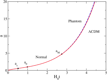
Figure 1: Temporal evolution of the scale factor in the Logotropic model (blue) as compared to the $\Lambda$CDM model (red).

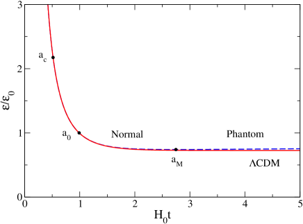
Figure 2: Temporal evolution of the energy density in the Logotropic model (blue) as compared to the $\Lambda$CDM model (red).

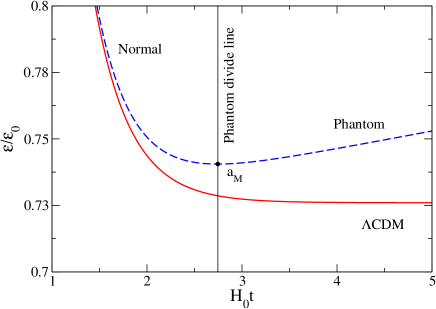
Figure 3: Zoom of Fig. 2. We have indicated the phantom divide line at which the energy density starts increasing with the scale factor in the Logotropic model.

The temporal evolutions of the energy density $\epsilon(t)$ and of the scale factor $a(t)$ are represented in Figs. 1-3. We have taken $B=3.53\times 10^{-3}$. The Universe starts at $t=0$ with a vanishing scale factor ($a=0$) and an infinite energy density ($\epsilon\rightarrow+\infty$). The Universe experiences a DM era followed by a DE era. In the DM era, the Universe is decelerating. The scale factor increases as $t^{2/3}$ and the energy density decreases as $t^{-2}$. This corresponds to the EdS solution. In the DE era, the Universe is accelerating. The Universe starts accelerating at $t_{c}=7.19\,{\rm Gyrs}$ (corresponding to $a_{c}=0.574$ and $\epsilon_{c}/\epsilon_{0}=2.17$). The energy density $\epsilon_{\rm m}$ associated with DM (actually the rest-mass energy of the DF) is equal to the energy density $\epsilon_{\rm de}$ associated with DE (actually the internal energy of the DF) at $t_{2}=9.63\,{\rm Gyrs}$ (corresponding to $a_{2}=0.723$ and $\epsilon_{2}/\epsilon_{0}=1.45$). The Logotropic model is very close to the $\Lambda$CDM model up to the present (the age of the Universe is $t_{0}=13.8\,{\rm Gyrs}$). However, in the far future, at $t_{M}=38.3\,{\rm Gyrs}$ (corresponding to $a_{M}=4.75$ and $\epsilon_{M}/\epsilon_{0}=0.7405$), the Logotropic Universe will become phantom. At that moment, the energy will increase with time as the Universe expands. Asymptotically, its energy density will increase as $t^{2}$ and the scale factor will have a super de Sitter behavior. The scale factor and the energy density will become infinite in infinite time. This corresponds to a little rip [40]. By contrast, in the $\Lambda$CDM model, the energy density of the Universe tends towards a constant $\epsilon_{\Lambda}$ and the scale factor has a de Sitter behavior.

Remark: The Logotropic model may break down before the Universe enters in the phantom regime because the speed of sound exceeds the speed of light at $t_{s}=34.5\,{\rm Gyrs}$ (corresponding to $a_{s}=3.77$ and $\epsilon_{s}/\epsilon_{0}=0.741$), i.e., before the Universe becomes phantom ($a_{s}=a_{M}/2^{1/3}$). Note that the speed of sound $c_{s}$ defined by $c_{s}^{2}=P^{\prime}(\epsilon)c^{2}=c^{2}/((a_{M}/a)^{3}-1)$ is real for $a<a_{M}$ (i.e., when the Universe is normal) and imaginary for $a>a_{M}$ (i.e., when the Universe is phantom). We must remain cautious, however, about these considerations because it has been known for a long time that the propagation of signals with a speed bigger than the speed of light is possible and does not contradict the general principles of physics [61].

2.8 The two fluids model

In the Logotropic model developed in [50] and discussed previously, the Universe is made of a single DF with an equation of state given by Eq. (2.14) unifying DM and DE. It is interesting to consider a related model in which the Universe is made of two noninteracting fluids, a DM fluid with a pressureless equation of state

$$P_{\rm m}=0,\qquad\frac{\epsilon_{\rm m}}{\epsilon_{0}}=\frac{\Omega_{\rm m0}}{a^{3}},\qquad\epsilon_{\rm m}=\rho_{\rm m}c^{2},$$ (2.61)

and a DE fluid with an affine equation of state

$$P_{\rm de}=-\epsilon_{\rm de}-A,\qquad\frac{\epsilon_{\rm de}}{\epsilon_{0}}=\Omega_{\rm de0}(1+3B\ln a),\qquad\epsilon_{\rm de}=-A\ln\rho_{\rm de}+C,$$ (2.62)

where we have defined $B=A/\Omega_{\rm de0}\epsilon_{0}$ as before. In order to obtain the second and third expressions of each line, we have solved the equation of continuity (2.1) and the first law of thermodynamics (2.8) for each individual fluid described by the corresponding equation of state. These two fluids correspond to the asymptotic behaviors of the LDF in the early and late Universe respectively. Their equations of state parameters are

$$w_{\rm m}=\frac{P_{\rm m}}{\epsilon_{\rm m}}=0,\qquad w_{\rm de}=\frac{P_{\rm de}}{\epsilon_{\rm de}}=-1-\frac{B}{1+3B\ln a}.$$ (2.63)

The function $w_{\rm de}(a)$ starts from $-1$ at $a_{i}=0$, increases, tends towards $+\infty$ as $a\rightarrow a_{*}^{-}=9.775\times 10^{-42}$, tends towards $-\infty$ as $a\rightarrow a_{*}^{+}=9.775\times 10^{-42}$, increases and tends slowly (logarithmically) towards $-1^{-}$ for $a\rightarrow+\infty$. For typical values of $a$, the parameter $w_{\rm de}$ has an approximately constant value $\sim w_{\rm de0}=-1-B=-1.00353$, due to its slow (logarithmic) dependence on the scale factor.

Summing the energy contribution of these two fluids, we obtain

$$\frac{\epsilon}{\epsilon_{0}}=\frac{\Omega_{\rm m0}}{a^{3}}+\Omega_{\rm de0}(1+3B\ln a)$$ (2.64)

which coincides with Eq. (2.32). The total pressure $P=P_{\rm m}+P_{\rm de}=P_{\rm de}$ reduces to the pressure of DE and can be written as

$$\frac{P}{\Omega_{\rm de0}\epsilon_{0}}=-B-1-3B\ln a$$ (2.65)

which coincides with Eq. (2.30). Therefore, at the background level, the two fluids model is equivalent to the single LDF model. However, despite this equivalence, the one fluid model and the two fluids model present some differences:

(i) In the two fluids model, the DE fluid exists only for $a>a_{*}=e^{-1/3B}=9.775\times 10^{-42}$ because we must require its energy density to be positive ($\epsilon_{\rm de}\geq 0$). In the one fluid model, $\epsilon_{\rm de}$ can be negative because it actually represents the internal energy $u$ of the DF which can be positive or negative (as long as the total energy $\epsilon=\epsilon_{\rm m}+\epsilon_{\rm de}$ is positive). However, since $a_{*}$ is extremely small, corresponding to an epoch where our study is not applicable anyway, this difference is not important.

(ii) In the two fluids model, the pressure, which reduces to the pressure of DE is given by $P=A\ln\rho_{\rm de}+C$. Therefore, it depends on the logarithm of the rest-mass density of DE, $\rho_{\rm de}$, not on the total rest-mass density, $\rho$, as in the one fluid model.

(iii) In the two fluids model, there is no way to predict the value of the constant $B$ while this is possible in the one fluid model (see Sec. 2.5).

(iv) Defining the speed of sound by $(c_{s}^{2}/c^{2})_{i}=P^{\prime}(\epsilon_{i})$ for each species $i\in\{{\rm m,de}\}$ in the two fluids model, we find from Eqs. (2.61) and (2.62) that DM has a vanishing speed of sound $(c_{s})_{\rm m}=0$ and that DE has an imaginary speed of sound $(c_{s}^{2}/c^{2})_{\rm de}=-1$. By contrast, in the one fluid model, defining the speed of sound by $(c_{s}^{2}/c^{2})=P^{\prime}(\epsilon)$, the LDF has a real nonzero speed of sound $(c_{s}^{2}/c^{2})_{\rm LDF}=1/((a_{M}/a)^{3}-1)$ in the normal Universe ($a<a_{M}=4.75$) [50]. This difference has several important consequences:

(iv-a) Even if the one fluid and two fluids models are equivalent at the background level, they differ at the level of the perturbations.

(iv-b) Since the LDF has a nonzero speed of sound, it has a nonvanishing Jeans length. This Jeans length may account for the minimum size of DM halos in the Universe as discussed in [50]. In the two fluids model, DM has a vanishing speed of sound (like CDM) so there is no minimum size of DM halos. Therefore, DM halos should form at all scales. This should lead to an abundance of small-scale structures which are not observed. This is the so-called missing satellite problem [15].

(iv-c) The pressure of the LDF can prevent gravitational collapse and lead to DM halos with a core. In the two fluids model, DM has a vanishing pressure (like CDM) so that nothing prevents gravitational collapse. This leads to cuspy DM halos that are in contradiction with observations. This is the so-called cusp problem [16].

3 Statefinders of the Logotropic model

3.1 Definition

Sahni et al. [62] suggested a very useful way of comparing and distinguishing different cosmological models by introducing the statefinders $\{q,r,s\}$ defined by

$$q=-\frac{{\ddot{a}}a}{{\dot{a}}^{2}},\qquad r=\frac{\dddot{a}}{aH^{3}},\qquad s=\frac{r-1}{3(q-1/2)},$$ (3.1)

where $q$ is the deceleration parameter and $r$ is the jerk parameter. Introducing the Hubble parameter $H=\dot{a}/a$, we obtain

$$q=-1-\frac{aH^{\prime}}{H},$$ (3.2)

$$r=a^{2}\left(\frac{H^{\prime}}{H}\right)^{2}+4a\frac{H^{\prime}}{H}+1+a^{2}\frac{H^{\prime\prime}}{H},$$ (3.3)

where prime denotes a derivative with respect to $a$.

For the Logotropic model, the Hubble parameter is given by

$$\frac{H}{H_{0}}=\sqrt{\frac{\Omega_{\rm m0}}{a^{3}}+\Omega_{\rm de0}(1+3B\ln a)}.$$ (3.4)

After simplification, we obtain the simple analytical expressions

$$q=\frac{1}{2}-\frac{3\Omega_{\rm de0}}{2}\frac{B+1+3B\ln a}{\frac{\Omega_{\rm m0}}{a^{3}}+\Omega_{\rm de0}(1+3B\ln a)},$$ (3.5)

$$r=1+\frac{9B\Omega_{\rm de0}}{2}\frac{1}{\frac{\Omega_{\rm m0}}{a^{3}}+\Omega_{\rm de0}(1+3B\ln a)},$$ (3.6)

$$s=-\frac{B}{B+1+3B\ln a}.$$ (3.7)

We note the remarkable fact that the parameter $s$ is a universal function of $a$ and $B$ (it does not depend on the present fraction of DM and DE). We now consider asymptotic limits of these expressions. For $a\rightarrow 0$:

$$q\simeq\frac{1}{2}-\frac{3\Omega_{\rm de0}}{2\Omega_{\rm m0}}(B+1+3B\ln a)a^{3},$$ (3.8)

$$r\simeq 1+\frac{9B\Omega_{\rm de0}}{2\Omega_{\rm m0}}a^{3}.$$ (3.9)

The Logotropic Universe begins at $t_{i}=0$ corresponding to $a_{i}=0$ and $\epsilon_{i}\rightarrow+\infty$ (big bang). At that point $q_{i}=1/2$, $r_{i}=1$ and $s_{i}=0$. This corresponds to the EdS limit. For $a\rightarrow+\infty$:

$$q\simeq-1-\frac{3B}{2(1+3B\ln a)},$$ (3.10)

$$r\simeq 1+\frac{9B}{2(1+3B\ln a)}.$$ (3.11)

Therefore, $q\rightarrow-1$, $r\rightarrow 1$ and $s\rightarrow 0$. This corresponds to the super dS limit (little rip).

For the $\Lambda$CDM model ($B=0$) we recover the well-known expressions

$$q=\frac{1}{2}-\frac{3\Omega_{\rm de0}}{2}\frac{1}{\frac{\Omega_{\rm m0}}{a^{3}}+\Omega_{\rm de0}},\qquad r=1,\qquad s=0.$$ (3.12)

For $a\rightarrow 0$:

$$q\simeq\frac{1}{2}-\frac{3\Omega_{\rm de0}}{2\Omega_{\rm m0}}a^{3}.$$ (3.13)

For $a\rightarrow+\infty$:

$$q\rightarrow-1.$$ (3.14)

The $\Lambda$CDM model Universe begins at $t_{i}=0$ corresponding to $a_{i}=0$ and $\epsilon_{i}\rightarrow+\infty$ (big bang). At that point $q_{i}=1/2$, $r_{i}=1$ and $s_{i}=0$. This corresponds to the EdS limit. On the other hand, for $a\rightarrow+\infty$ we get $q\rightarrow-1$, $r\rightarrow 1$ and $s\rightarrow 0$. This corresponds to the dS limit. We note that the statefinders of the Logotropic and $\Lambda$CDM models coincide for $a\rightarrow 0$ and $a\rightarrow+\infty$ but they differ in between.

3.2 Particular values

We now provide the values of the statefinders at particular points of interest in the Logotropic model.

(i) The pressure of the Logotropic Universe vanishes ($w=0$) at

$$a_{w}=e^{-\frac{1+B}{3B}}.$$ (3.15)

At that point

$$q_{w}=\frac{1}{2},$$ (3.16)

$$r_{w}=1+\frac{9B\Omega_{\rm de0}}{2[\Omega_{\rm m0}e^{(1+B)/B}-B\Omega_{\rm de0}]},$$ (3.17)

$$s_{w}=\infty.$$ (3.18)

Numerically

$$a_{w}=7.00\times 10^{-42},\qquad\epsilon_{w}/\epsilon_{0}=7.97\times 10^{122},\qquad H_{0}t_{w}=2.36\times 10^{-62},$$ (3.19)

$$q_{w}=0.5,\qquad r_{w}=1.00,\qquad s_{w}=\infty.$$ (3.20)

We note that the parameter $s$ diverges at $a_{w}=7.00\times 10^{-42}$ while its value in the $\Lambda$CDM model is always $s=0$. However, this is essentially a mathematical curiosity since the Logotropic model (which is a unification of DM and DE) may not be justified at such small scale factors (see footnote 11).

(ii) The Logotropic Universe accelerates ($q\geq 0$) at the point $a_{c}$ defined implicitly by the relation

$$B=\frac{\frac{\Omega_{\rm m0}}{\Omega_{\rm de0}a_{c}^{3}}-2}{3(1+2\ln a_{c})}.$$ (3.21)

The function $a_{c}(B)$ is studied in [50]. At that point

$$q_{c}=0,$$ (3.22)

$$r_{c}=1+\frac{9B\Omega_{\rm de0}}{2[\frac{\Omega_{\rm m0}}{a_{c}^{3}}+\Omega_{\rm de0}(1+3B\ln a_{c})]},$$ (3.23)

$$s_{c}=-\frac{2}{3}(r_{c}-1)=-\frac{B}{B+1+3B\ln a_{c}}.$$ (3.24)

Numerically

$$a_{c}=0.574,\qquad\epsilon_{c}/\epsilon_{0}=2.17,\qquad H_{0}t_{c}=0.515,$$ (3.25)

$$q_{c}=0,\qquad r_{c}=1.005,\qquad s_{c}=-0.00354.$$ (3.26)

For the $\Lambda$CDM model ($B=0$), we have

$$a_{c}=\left(\frac{\Omega_{\rm m0}}{2\Omega_{\rm de0}}\right)^{1/3}.$$ (3.27)

Numerically

$$a_{c}=0.574,\qquad\epsilon_{c}/\epsilon_{0}=2.18,\qquad H_{0}t_{c}=0.515,$$ (3.28)

$$q_{c}=0,\qquad r_{c}=1,\qquad s_{c}=0.$$ (3.29)

(iii) The current values of the statefinders ($a=1$) in the Logotropic model are

$$q_{0}=\frac{1}{2}-\frac{3\Omega_{\rm de0}}{2}({B+1}),$$ (3.30)

$$r_{0}=1+\frac{9B\Omega_{\rm de0}}{2},$$ (3.31)

$$s_{0}=-\frac{B}{B+1}.$$ (3.32)

We emphasize that $s_{0}$ depends only on $B$. Therefore, the present value of $s$ unequivocally determines $B$ independently of the values of $\Omega_{\rm m0}$ and $H_{0}$. Numerically

$$a_{0}=1,\qquad\epsilon_{c}/\epsilon_{0}=1,\qquad H_{0}t_{c}=0.989,$$ (3.33)

$$q_{0}=-0.593,\qquad r_{0}=1.01,\qquad s_{0}=-0.00352.$$ (3.34)

For the $\Lambda$CDM model ($B=0$), we have

$$a_{0}=1,\qquad\epsilon_{c}/\epsilon_{0}=1,\qquad H_{0}t_{c}=0.989,$$ (3.35)

$$q_{0}=-0.589,\qquad r_{0}=1,\qquad s_{0}=0.$$ (3.36)

In the $\Lambda$CDM model, $s=0$ exactly while $s_{0}=-0.00352$ in the Logotropic model. Therefore, the observation of a small negative value of $s$ would be in favor of the Logotropic model. Since $B>0$, we predict that the distribution of measured values of $s$ about $s=0$ should be disymmetric and should favor negatives values of $s$ with respect to positive ones. However, it is not clear if this slight asymmetry can be observed with current precision of measurements.

(iv) The Logotropic Universe becomes phantom ($w=-1$) at

$$a_{M}=\left(\frac{\Omega_{\rm m0}}{B\Omega_{\rm de0}}\right)^{1/3}.$$ (3.37)

At that point

$$q_{M}=-1,$$ (3.38)

$$r_{M}=1+\frac{9B}{2[B+1+B\ln(\Omega_{\rm m0}/B\Omega_{\rm de0})},$$ (3.39)

$$s_{M}=-\frac{2}{9}(r_{M}-1)=-\frac{B}{B+1+B\ln(\Omega_{\rm m0}/B\Omega_{\rm de0})}.$$ (3.40)

Numerically

$$a_{M}=4.75,\qquad\epsilon_{M}/\epsilon_{0}=0.7405,\qquad H_{0}t_{M}=2.745,$$ (3.41)

$$q_{M}=-1,\qquad r_{M}=1.015,\qquad s_{M}=-0.00346.$$ (3.42)

3.3 The functions $q(a)$, $r(a)$ and $s(a)$

The differences between the Logotropic model and the $\Lambda$CDM model are apparent on Figs. 4 and 5 where we plot individually $q$, $r$ and $s$ as a function of the scale factor $a$.

The function $q(a)$ (see Fig. 4) has been studied in detail in [50] so we remain brief. This function starts from $q_{i}=1/2$ at $a_{i}=0$, increases, reaches a maximum $q_{\rm max}=0.5+1.77\times 10^{-126}$ at $a^{\prime}\simeq e^{-(2B+1)/3B}=5.02\times 10^{-42}$, decreases, takes the value $q=1/2$ at $a_{w}=7.00\times 10^{-42}$ (at that point the pressure vanishes), takes the value $q=0$ at $a_{c}=0.574$ (at that point the Universe starts accelerating), takes the value $q=-1$ at $a_{M}=4.75$ (at that point the Universe becomes phantom), reaches a minimum $q_{\rm min}=-1.005$ at $a^{\prime\prime}=31.6$ (approximately $a^{\prime\prime}\simeq[(2B+1)\Omega_{\rm m0}/B^{2}\Omega_{\rm de0}]^{1/3}$), increases and tends slowly (logarithmically) towards $-1^{-}$ for $a\rightarrow+\infty$. By comparison, for the $\Lambda$CDM model, the function $q(a)$ starts from $q_{i}=1/2$ at $a_{i}=0$, decreases monotonically, takes the value $q=0$ at $a_{c}=0.574$, and tends towards $-1^{+}$ for $a\rightarrow+\infty$. The evolution of the equation of state parameter $w(a)$ can be obtained straightforwardly from the evolution of $q(a)$ by using the relation of Eq. (2.5).

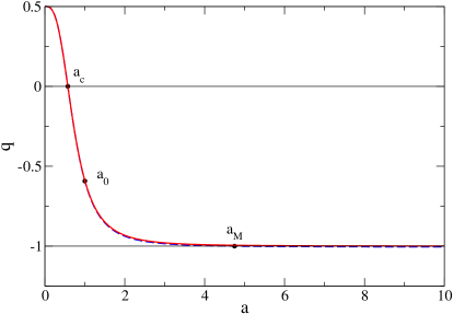
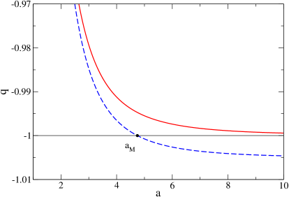
Figure 4: The deceleration parameter $q$ as a function of the scale factor for the Logotropic model (blue) and for the $\Lambda$CDM model (red). The right panel is a zoom close to the point where the Logotropic Universe becomes phantom.

The function $r(a)$ (see Fig. 5, left panel) starts from $r_{i}=1$ at $a_{i}=0$, increases, reaches a maximum $r_{M}=1.015$ at $a_{M}=4.75$ (at that point the Universe becomes phantom) and decreases slowly (logarithmically) towards $1^{+}$ for $a\rightarrow+\infty$.

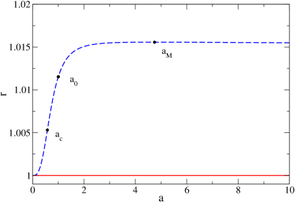
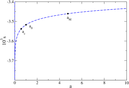
Figure 5: Left: Parameter $r$ as a function of the scale factor for the Logotropic model (blue) and for the $\Lambda$CDM model (red). Right: Parameter $s$ (multiplied by $1000$) as a function of the scale factor for the Logotropic model. For the $\Lambda$CDM model, $s=0$.

The function $s(a)$ (see Fig. 5, right panel) starts from $s_{i}=0$ at $a_{i}=0$, increases, tends towards $+\infty$ as $a\rightarrow a_{w}^{-}=7.00\times 10^{-42}$, tends towards $-\infty$ as $a\rightarrow a_{w}^{+}=7.00\times 10^{-42}$, increases and tends slowly (logarithmically) towards $0^{-}$ for $a\rightarrow+\infty$. Since the singularity at $a=a_{w}$ occurs in the very early Universe where the Logotropic model may not be valid, we have not represented it on the figure. We note that for typical values of $a$, the parameter $s$ has an approximately constant value $\sim-3.53\times 10^{-3}$, due to its slow (logarithmic) dependence on the scale factor, which corresponds to the value of the dimensionless Logotropic temperature $B$ (with the opposite sign).

3.4 The $qr$ and $sr$ planes

We plot the evolution trajectories of the Logotropic and $\Lambda$CDM models in the $qr$ plane in Fig. 6. The Logotropic model and the $\Lambda$CDM model have different trajectories but evolve from a matter dominated phase (EdS) corresponding to the point $(1/2,1)$ in the $qr$ plane to the de Sitter phase (for the $\Lambda$CDM model) or to the super de Sitter phase (for the Logotropic model) corresponding to the point $(-1,1)$ in the $qr$ plane. In this representation, the $\Lambda$CDM model forms a segment while the evolution of the Logotropic model is more complex. We can discriminate the Logotropic model from the $\Lambda$CDM model by observing that the dashed line (Logotropic model) runs above the solid line ($\Lambda$CDM model) in the $qr$ plane. On the other hand, as revealed by the zoom of Fig. 6-b, the dashed line (Logotropic model) crosses the phantom divide line $q=-1$, contrary to the solid line ($\Lambda$CDM model).

We have also represented the $sr$ plane in Fig. 7. In this representation, the $\Lambda$CDM model reduces to a point $(0,1)$ while the Logotropic model has a more complicated evolution around that point. As explained previously, the departure of the current value of $s$ from the $\Lambda$CDM value $s=0$ is a direct measure of the dimensionless Logotropic temperature $B$ since $s_{0}=-B/(B+1)$.

Despite minute differences in their evolution trajectories, the Logotropic model and the $\Lambda$CDM model are extremely close to each other so they could be distinguished from observations only if the cosmological parameters are calculated with a high precision of the percent level. This precision is not reached by present-day observations. However, even if the Logotropic model and the $\Lambda$CDM model are extremely close to each other at the cosmological scale, they behave very differently at small scales as discussed in the Introduction.

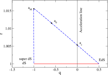
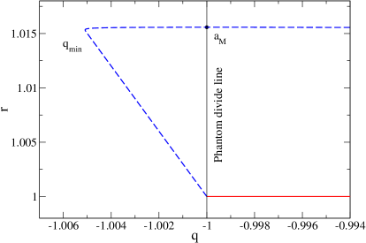
Figure 6: The $qr$ trajectory for the Logotropic model (blue) and for the $\Lambda$CDM model (red). The right panel is a zoom close to the phantom divide line. We have indicated the acceleration line where $q=0$ and the phantom divide line where $q=-1$. We have also indicated the point where $r$ is maximum and the point where $q$ is minimum.

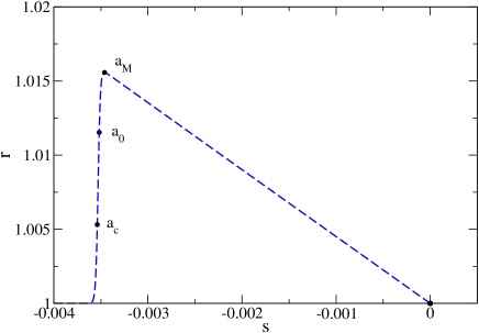
Figure 7: The $sr$ trajectory for the Logotropic model. For the $\Lambda$CDM model, $(s,r)=(0,1)$.

4 Fine comparison between the Logotropic and $\Lambda$CDM models

In this section, we present observational constraints on the Logotropic model using the latest observational data from Planck 2015+Lensing+BAO+JLA+HST (see [10] for details of the data sets) and compare them with the $\Lambda$CDM model. To that purpose, we consider DM and DE as two separate/non-interacting fluids as in Sec. 2.8, and use the value of $B$ given in Eq. (2.50). We also assume that the Universe is flat in agreement with the observations of the CMB [9, 10].

4.1 Background and perturbation equations

For the purpose of observational constraints, we write the expansion history of the Logotropic model as

$$H=H_{0}\sqrt{\Omega_{\rm r0}(1+z)^{4}+\Omega_{\rm b0}(1+z)^{3}+\Omega_{\rm dm0}(1+z)^{3}+\Omega_{\rm de0}(1-3B\ln(1+z))},$$ (4.1)

where $\Omega_{\rm r0}$, $\Omega_{\rm b0}$, $\Omega_{\rm dm0}$ and $\Omega_{\rm de0}$ are the present-day values of density parameters of radiation, baryonic matter, DM and DE respectively with $\Omega_{\rm m0}=\Omega_{\rm b0}+\Omega_{\rm dm0}$ and $\Omega_{\rm r0}+\Omega_{\rm b0}+\Omega_{\rm dm0}+\Omega_{\rm de0}=1$. Furthermore, $z=a^{-1}-1$ is the redshift. We use the following perturbation equations for the density contrast and velocity divergence in the synchronous gauge:

$$\dot{\delta}_{i} = -(1+w_{i})(\theta_{i}+\frac{\dot{h}}{2})+\frac{\dot{w}_{i}}{1+w_{i}}\delta_{i}-3\mathcal{H}(c^{2}_{s,\rm eff}-c^{2}_{s,\rm ad})\left[\delta_{i}+3\mathcal{H}(1+w_{i})\frac{\theta_{i}}{k^{2}}\right],$$ (4.2)

$$\dot{\theta}_{i} = -\mathcal{H}(1-3c^{2}_{s,\rm eff})\theta_{i}+\frac{c^{2}_{s,\rm eff}}{1+w_{i}}k^{2}\delta_{i}-k^{2}\sigma_{i},$$ (4.3)

following the notations of [63, 64]. The adiabatic sound speed is given by

$$c^{2}_{s,\rm ad}=\frac{\dot{p}_{i}}{\dot{\rho}_{i}}=w_{i}-\frac{\dot{w}_{i}}{3\mathcal{H}(1+w_{i})},$$ (4.4)

where $c^{2}_{s,\rm eff}$ is the effective sound speed in the rest frame of the $i$th fluid. In general, $c^{2}_{s,\rm eff}$ is a free model parameter, which measures the entropy perturbations through its difference to the adiabatic sound speed via the relation $w_{i}\Gamma_{i}=(c^{2}_{s,\rm eff}-c^{2}_{s,\rm ad})\delta^{\rm rest}_{i}$. Thus, $w_{i}\Gamma_{i}$ characterizes the entropy perturbations. Furthermore, $\delta^{\rm rest}_{i}=\delta_{i}+3\mathcal{H}(1+w_{i})\theta_{i}/k^{2}$ gives a gauge-invariant form for the entropy perturbations. With these definitions, the microscale properties of the energy component are characterized by three quantities, i.e., the equation of state parameters $w_{i}$, the effective sound speed $c^{2}_{s,\rm eff}$ and the shear perturbation $\sigma_{i}$. In this work, we assume zero shear perturbations for the DE. Finally, for the DM and DE equation of state parameters, we take the values of $w_{\rm m}$ and $w_{\rm de}$ defined by Eq. (2.63).

4.2 Observational constraints

We use the observational data from Planck 2015+Lensing+BAO+JLA+HST to perform a global fitting to the model parameter space of the Logotropic and $\Lambda$CDM models

$$P\equiv\{\Omega_{\rm b}h^{2},\Omega_{\rm c}h^{2},100\theta_{\rm MC},\tau,n_{\rm s},\ln[10^{10}A_{\rm s}]\}$$

via the Markov chain Monte Carlo (MCMC) method. Here, $\Omega_{\rm b}h^{2}$ and $\Omega_{\rm c}h^{2}$ ($\Omega_{\rm c}$ was previously denoted $\Omega_{\rm dm}$) are respectively the baryon and cold DM densities today, $\theta_{\rm MC}$ is an approximation to the angular size of the sound horizon at the time of decoupling, $\tau$ is the Thomson scattering optical depth due to reionization, $n_{\rm s}$ is the scalar spectrum power-law index and $\log[10^{10}A_{\rm s}]$ is the log power of the primordial curvature perturbations [9]. We modified the publicly available cosmoMC package [65] to include the perturbations of DE in accordance with Eqs. (4.2) and (4.3). Assuming suitable priors on various model parameters, we obtained the constraints on the parameters of the Logotropic and $\Lambda$CDM models displayed in Table 1.

Table 1: Constraints on the parameters of the Logotropic and $\Lambda$CDM models from Planck 2015+Lensing+BAO+JLA+HST data. The parameter $H_{0}$ is in the units of km s^-1 Mpc^-1

Model $\rightarrow$	Logotropic		$\Lambda$CDM
Parameter	Mean value with 68% C.L.	Bestfit value	Mean value with 68% C.L.	Bestfit value
$\Omega_{\rm b}h^{2}$	$0.02231\pm 0.00014$	$0.02234$	$0.02232\pm 0.00014$	$0.02232$
$\Omega_{\rm c}h^{2}$	$0.1186\pm 0.0010$	$0.1176$	$0.1184\pm 0.0010$	$0.1181$
$100\theta_{\rm MC}$	$1.04094\pm 0.00030$	$1.04098$	$1.04095\pm 0.00029$	$1.04107$
$\tau$	$0.067\pm 0.012$	$0.069$	$0.068\pm 0.012$	$0.078$
${\rm{ln}}(10^{10}A_{\rm s})$	$3.065\pm 0.023$	$3.069$	$3.067\pm 0.023$	$3.087$
$n_{\rm s}$	$0.9671\pm 0.0040$	$0.9705$	$0.9676\pm 0.0039$	$0.9681$
$\Omega_{\rm m0}$	$0.3068\pm 0.0060$	$0.3014$	$0.3070\pm 0.0061$	$0.3049$
$H_{0}$	$67.93\pm 0.45$	$68.30$	$67.87\pm 0.46$	$68.02$

In Fig. 8, we show one-dimensional marginalized distributions of individual parameters and two-dimensional contours with $68\%$ C.L. and $95\%$ C.L. for the model parameters under consideration. The CMB TT power spectra and matter power spectra at redshift $z=0$ for the $\Lambda$CDM and Logotropic models are displayed in Fig. 9, where the relevant parameters are fixed to their best fit values as given in Table 1. From Table 1, Fig. 8 and Fig. 9, we notice that there is no significant difference between the $\Lambda$CDM and Logotropic models at the present epoch, as expected. However, the Logotropic model will behave differently from the $\Lambda$CDM model in the future evolution of the Universe as the logarithmic term will eventually be significant for larger values of $a$. In the following subsection, we quantify this difference by testing the evolutionary behavior of some parameters pertaining to the two models under consideration.

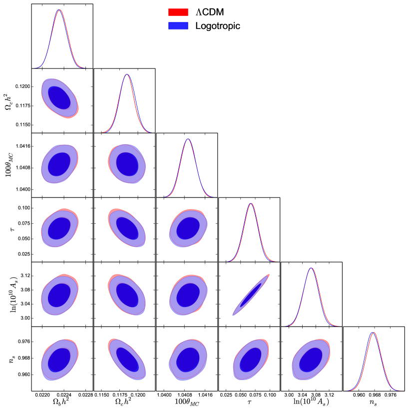
Figure 8: The one-dimensional marginalized distributions of individual parameters and two-dimensional contours with $68\%$ C.L. and $95\%$ C.L.

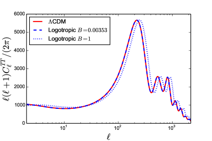
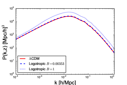
Figure 9: The CMB TT power spectra (left panel) and the matter power spectra (right panel) at redshift $z=0$ for the $\Lambda$CDM (full red line) and Logotropic (dashed blue line) models, where the relevant parameters are fixed to their best fit values given in Table 1. The two curves are almost indistinguishable, implying that the Logotropic model can account for cosmological observations as well as the $\Lambda$CDM model. For comparison, we have plotted the Logotropic model with $B=1$ (blue dotted line) which presents a strong deviation from the $\Lambda$CDM model. This confirms that the parameter $B$ must be sufficiently small, such as the predicted value $B=3.53\times 10^{-3}$, to account for the observations [50, 51].

4.3 Statefinders and behavior of dark energy

The statefinder analysis is done as follows. The evolution trajectories of the $\{q,r\}$ and $\{s,r\}$ pairs are plotted in $qr$ and $sr$ planes. Since the jerk parameter of the $\Lambda$CDM model is $r=1$ whilst $s=0$, the $\Lambda$CDM model is represented by the point $(0,1)$ in the $sr$ plane. On the other hand, $q$ varies from $1/2$ to $-1$ in the $\Lambda$CDM model. Therefore, the $qr$ trajectory for the $\Lambda$CDM model is a straight line segment going from $(1/2,1)$ to $(-1,1)$ in the $qr$ plane. By plotting the $qr$ and $sr$ trajectories for the models under consideration, one can easily observe the difference between their evolutionary behavior.

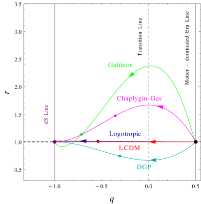
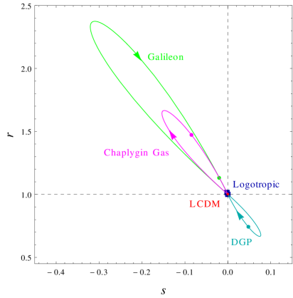
Figure 10: The left and right panels respectively show the evolution of the $qr$ and $sr$ trajectories for various cosmological models. In both panels, the blue curve corresponds to the Logotropic model. Red, cyan, magenta and green curves stand for $\Lambda$CDM, DGP, Chaplygin gas and Galileon models, respectively. The direction of evolution is shown by the arrows on the curves while the dots on the curves are used to indicate the present values of the corresponding $\{q,r\}$ and $\{s,r\}$ pairs. All the models under consideration evolve from the matter dominated (EdS) phase (black dot $(1/2,1)$ in the $qr$ plane) to the de Sitter phase (purple dot $(-1,1)$ in the $qr$ plane). The Logotropic model shows a good consistency with the $\Lambda$CDM model till the blue dot on the $qr$ curve. But later on, it is visible that the blue curve departs from the red line (see the zoom in Fig. 11).

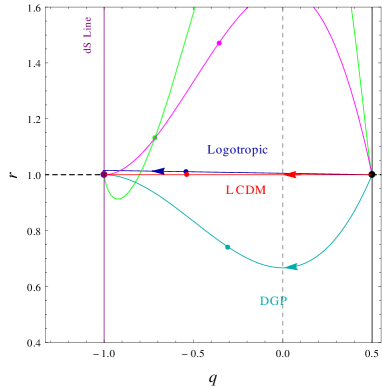
Figure 11: Zoom of Fig. 10 enlightening the difference between the Logotropic and $\Lambda$CDM models.

We plot the evolution trajectories of the Logotropic and $\Lambda$CDM models in the $qr$ and $sr$ planes in the left and right panels of Fig. 10 by considering the best fit values of the model parameters given in Table 1 from observations. For the sake of comparison, we also plot the $qr$ and $sr$ trajectories of some popular models such as the DGP [34], Chaplygin gas [41] and Galileon [37] models (see [66] for the statefinder analysis of these models).

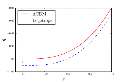
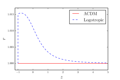
Figure 12: The left and right panels respectively show the variation of $q$ and $r$ vs $z$ in the $\Lambda$CDM and Logotropic models.

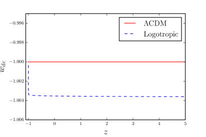
Figure 13: Variation of $s$ vs $z$ in the $\Lambda$CDM and Logotropic models (left). Variation of $w_{\rm de}$ vs $z$ in the $\Lambda$CDM and Logotropic models (right).

We see that all the models have different evolution trajectories but evolve from the matter dominated (EdS) phase (black dot $(1/2,1)$ in the $qr$ plane) to the de Sitter phase (purple dot $(-1,1)$ in the $qr$ plane). Of all these models, the Logotropic model is the closest to the $\Lambda$CDM model. We can discriminate the Logotropic model from the $\Lambda$CDM model by observing that the blue curve (Logotropic model) evolves differently from the red line ($\Lambda$CDM model) in the $qr$ plane. The blue curve can be seen to run slightly above the red line, especially after the blue dot corresponding to the current Universe. In addition, the blue curve crosses the de Sitter line $q=-1$ (phantom divide) before finally converging towards the de Sitter point $(-1,1)$, as explained in Sec. 3. To display this behavior more clearly, we plot $q$, $r$ and $s$ separately in Figs. 12 and 13 (left) where the departure of the Logotropic model from the $\Lambda$CDM model can clearly be observed in the future evolution of the Universe.

We numerically find that the transition of the Universe from deceleration to acceleration in the $\Lambda$CDM model takes place at $z_{c}=0.667$ while in the Logotropic model the transition redshift is $z_{c}=0.658$.

In Fig. 13 (right), we show the evolution of the effective DE equation of state parameter $w_{\rm de}$ defined by Eq. (2.63) vs $z$ in the $\Lambda$CDM and Logotropic models. The effective DE equation of state parameter $w_{\rm de}$ stays less than $-1$ during the evolution of the Logotropic Universe indicating the phantom nature of DE in the Logotropic model (its current value is $w_{\rm de0}=-1-B=-1.00353$). In the $\Lambda$CDM model, $w_{\rm de}=-1$.

In Figs. 14, we show the evolution of the equation of state parameter $w$ defined by Eq. (2.34) vs $z$ in the $\Lambda$CDM and Logotropic models. We note that $w$ in the Logotropic model is close to $0$ at large redshifts, decreases (its current value is $w_{0}=-0.7011$), drops below $-1$ at $z_{M}=-0.798$, reaches its minimum $w_{\rm min}=-1.003$ at $z^{\prime\prime}=-0.968$, and asymptotically tends towards $-1^{-}$ as $z\rightarrow-1$. Thus, a phantom flip signature is observed in the future evolution of the Logotropic Universe, which is not the case in the $\Lambda$CDM model ($w$ starts from $0$ and decreases monotonically towards $-1^{+}$ as $z\rightarrow-1$; its current value is $w_{0}=-0.6951$).

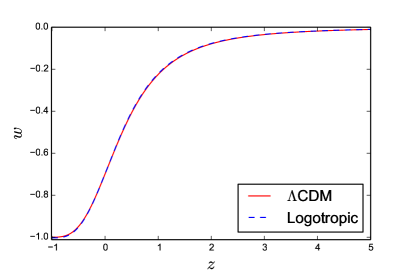
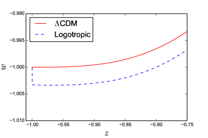
Figure 14: Variation of $w$ vs $z$ in the $\Lambda$CDM and Logotropic models.

4.4 Numerical applications

In this section, we provide the values of some quantities of cosmological interest at different epochs in the evolution of the Universe (see Table 2). We make the numerical application for $B=0$ corresponding to the $\Lambda$CDM model (see Sec. 2.4), and for $B=3.53\times 10^{-3}$ corresponding to the Logotropic model (see Sec. 2.5). We take the values of the cosmological parameters $H_{0}$ and $\Omega_{\rm m0}$ obtained from observations (see Table 1).

	$B=0$ ($\Lambda$CDM)	$B=3.53\times 10^{-3}$
$a_{w}$		$7.004\times 10^{-42}$
$(\epsilon/\epsilon_{0})_{w}$		$8.771\times 10^{122}$
$t_{w}$ (Gyrs)		$3.225\times 10^{-61}$
$q_{w}$		$1/2$
$w_{w}$		$0$
$r_{w}$		$1.000$
$s_{w}$		$\infty$
$a_{c}$	$0.6031$	$0.5998$
$(\epsilon/\epsilon_{0})_{c}$	$2.085$	$2.092$
$t_{c}$ (Gyrs)	$7.574$	$7.528$
$q_{c}$	$0$	$0$
$w_{c}$	$-1/3$	$-1/3$
$r_{c}$	$1$	$1.005$
$s_{c}$	$0$	$-0.003537$
$t_{0}$ (Gyrs)	$13.81$	$13.80$
$q_{0}$	$-0.5427$	$-0.5516$
$w_{0}$	$-0.6951$	$-0.7011$
$r_{0}$	$1$	$1.011$
$s_{0}$	$0$	$-0.003518$
$a_{M}$		$4.963$
$(\epsilon/\epsilon_{0})_{M}$		$0.7129$
$t_{M}$ (Gyrs)		$40.09$
$q_{M}$		$-1$
$w_{M}$		$-1$
$r_{M}$		$1.016$
$s_{M}$		$-0.003459$

Table 2: Numerical values of some quantities of cosmological interest (scale factor $a$, energy density $\epsilon$, time $t$, deceleration parameter $q$, equation of state parameter $w$, statefinders $r$ and $s$) at different periods of the evolution of the Universe. We recall that $t_{w}$ is the time at which the Logotropic pressure becomes negative, $t_{c}$ is the time at which the Universe accelerates, $t_{0}$ is the age of the Universe, and $t_{M}$ is the time at which the Logotropic Universe becomes phantom. These results update those of Table 1 of [50]. In this Table, we have neglected the contribution of radiation.

For the $\Lambda$CDM model, $\Omega_{\rm m0}=0.3049$, $\Omega_{\rm de0}=0.6951$, $H_{0}=68.02\,{\rm km}\,{\rm s}^{-1}\,{\rm Mpc}^{-1}=2.204\,10^{-18}\,{\rm s}^{-1}$, $\epsilon_{0}/c^{2}={3H_{0}^{2}}/{8\pi G}=8.691\times 10^{-24}\,{\rm g}\,{\rm m}^{-3}$, $\epsilon_{\rm m0}/c^{2}=\Omega_{\rm m0}\epsilon_{0}/c^{2}=2.650\times 10^{-24}\,{\rm g}\,{\rm m}^{-3}$, and $\epsilon_{\rm de0}/c^{2}=\Omega_{\rm de0}\epsilon_{0}/c^{2}=6.041\times 10^{-24}\,{\rm g}\,{\rm m}^{-3}$.

For the Logotropic model, $\Omega_{\rm m0}=0.3014$, $\Omega_{\rm de0}=0.6986$, $H_{0}=68.30\,{\rm km}\,{\rm s}^{-1}\,{\rm Mpc}^{-1}=2.213\,10^{-18}\,{\rm s}^{-1}$, $\epsilon_{0}/c^{2}={3H_{0}^{2}}/{8\pi G}=8.763\times 10^{-24}\,{\rm g}\,{\rm m}^{-3}$, $\epsilon_{\rm m0}/c^{2}=\Omega_{\rm m0}\epsilon_{0}/c^{2}=2.641\times 10^{-24}\,{\rm g}\,{\rm m}^{-3}$, and $\epsilon_{\rm de0}/c^{2}=\Omega_{\rm de0}\epsilon_{0}/c^{2}=6.122\times 10^{-24}\,{\rm g}\,{\rm m}^{-3}$. These values improve those given in Sec. 2.5. If we recompute $B$ and $A$ from Eq. (2.49) with these more accurate values we obtain

$$B=3.535\times 10^{-3},\qquad A=1.945\times 10^{-9}\,{\rm g}\,{\rm m}^{-1}\,{\rm s}^{-2}.$$ (4.5)

We see that the value of $B$ is not changed from the one given by Eq. (2.50). This shows the robustness of this value for the reason explained in Sec. 2.5. On the other hand, the value of $A$ is slightly changed since it depends more sensibly than $B$ on the measured values of $H_{0}$ and $\Omega_{\rm m0}$. However, we did not need the value of $A$ in the data analysis, so that our results are not altered.

5 Conclusion

In this paper, we have compared the Logotropic and $\Lambda$CDM models at large (cosmological) scales. This comparison is interesting because these two models are very different from each other on a theoretical point of view. As anticipated in [50, 51], the two models give results that are very close to each other up to the current epoch. Our detailed study shows that the difference is at the percent level (not smaller and not larger). This is smaller than present-day cosmological precision. Therefore, the two models are indistinguishable at present. Still, they will differ from each other in the far future, in about $25$ Gyrs, since the Logotropic Universe will become phantom unlike the $\Lambda$CDM Universe. The closeness of the results in the period where we can compare these two models with the observations implies that the Logotropic model is viable. Therefore, we cannot reject the possibility that our Universe will become phantom in the future. Indeed, the Logotropic model is an example of phantom Universe that is consistent with the observations since it leads to results that are almost indistinguishable from the $\Lambda$CDM model up to the current epoch. This is very different from the other models considered in Fig. 10 which deviate more strongly from the $\Lambda$CDM model. It may be argued that these models are not consistent with the observations since they are “too far” from the standard $\Lambda$CDM model.

In a sense, it is obvious that the Logotropic model produces results that are consistent with the observations since it depends on a parameter $B$ in such a way that the $\Lambda$CDM model is recovered for $B=0$. Therefore, by taking $B$ sufficiently small, we are guaranteed to reproduce the results of the $\Lambda$CDM model. However, an interest of the theory developed in [50, 51] is that $B$ is not a free parameter (unlike many other cosmological models that depend on one or several free parameters) but is fixed by physical considerations. Therefore, it can be interpreted as a sort of fundamental constant with the value $B=3.53\times 10^{-3}$, which is of the order of the inverse of the famous number $123$ occuring in the so-called cosmological constant problem. Intriguingly, the small but nonzero value of $B$ is related to the nonzero value of the Planck constant $\hbar$. This suggests that quantum mechanics plays a role at the cosmological scale in relation to DM and DE.

On the other hand, even if the Logotropic and $\Lambda$CDM models are close to each other at large (cosmological) scales, they differ at small (galactic) scales where the $\Lambda$CDM model poses problem. In particular, the Logotropic model is able to solve the CDM crisis (cusp problem, missing satellite problem…). Furthermore, it is able to explain the universality of the surface density $\Sigma_{0}=\rho_{0}r_{h}$ of DM halos and can predict its observed value $\Sigma_{0}=141\,M_{\odot}/{\rm pc}^{2}$ [52] without arbitrariness [50, 51].

For these reasons, the Logotropic model is a model of cosmological interest. We have obtained analytical expressions of the statefinders and shown that they slightly differ from the values of the $\Lambda$CDM model. The quantity of most interest seems to be the parameter $s$ whose predicted current value, $s_{0}=-B/(B+1)=-0.003518$, is directly related to the fundamental constant $B=3.53\times 10^{-3}$ of the Logotropic model independently of any other parameter.

Finally, an interesting aspect of our paper is to demonstrate explicitly that two cosmological models can be indistinguishable at large scales at the present time while they have a completely different evolution in the future since the Logotropic model leads to a phantom evolution (the energy density increases with the scale factor) unlike the $\Lambda$CDM model (the energy density tends to a constant). This result is interesting on a cosmological, physical and even philosophical point of view.

Appendix A Generalized thermodynamics and effective temperature

In this Appendix, we show that the Logotropic equation of state (2.14) can be related to a notion of (effective) generalized thermodynamics. In this approach, the constant $A$ can be interpreted as a generalized temperature called the Logotropic temperature [50, 51]. Generalized thermodynamics was introduced by Tsallis [60] and developed by numerous authors. The underlying idea of generalized thermodynamics is to notice that many results obtained with the Boltzmann entropy can be extended to more general entropic functionals. The formalism of generalized thermodynamics is mathematically consistent but the physical interpretation of the generalized entropy must be discussed in each case. We refer to [67, 68, 69] for recent books and reviews on the subject.

Let us consider a generalized entropy of the form

$$S=-\int C(\rho)\,d{\bf r},$$ (A.1)

where $C(\rho)$ is a convex function ($C^{\prime\prime}>0$). Following the fundamental principle of thermodynamics, the equilibrium state of the system in the microcanonical ensemble is obtained by maximizing the entropy at fixed mass $M=\int\rho\,d{\bf r}$ and energy $E=\frac{1}{2}\int\rho\Phi\,d{\bf r}$, where $\Phi({\bf r})=\int u(|{\bf r}-{\bf r}^{\prime}|)\rho({\bf r}^{\prime})\,d{\bf r}^{\prime}$ is the self-consistent mean field potential ($u(|{\bf r}-{\bf r}^{\prime}|)$ represents the binary potential of interaction between the particles which, in the present context, corresponds to the gravitational interaction). We write the variational problem for the first variations as

$$\delta S-\beta\delta E-\alpha\delta M=0,$$ (A.2)

where $\beta=1/T$ and $\alpha$ are Lagrange multipliers that can be interpreted as an inverse generalized temperature and a generalized chemical potential. Performing the variations, we obtain the relation

$$C^{\prime}(\rho)=-\beta\Phi({\bf r})-\alpha.$$ (A.3)

This integral equation fully determines the density $\rho({\bf r})$ since $C^{\prime}$ is invertible. Equation (A.3) may be rewritten as $\rho({\bf r})=F[\beta\Phi({\bf r})+\alpha]$ where $F(x)=(C^{\prime})^{-1}(-x)$. We note that, at equilibrium, the density is a function of the potential: $\rho=\rho(\Phi)$. Taking the derivative of Eq. (A.3) with respect to $\rho$, we get

$$\rho^{\prime}(\Phi)=-\frac{\beta}{C^{\prime\prime}(\rho)}.$$ (A.4)

Equation (A.3) determines the equilibrium distribution $\rho({\bf r})=F[\beta\Phi({\bf r})+\alpha]$ with $F(x)=(C^{\prime})^{-1}(-x)$ for a given entropy $C(\rho)$. Inversely, if the equilibrium distribution is characterized by a relation of the form $\rho({\bf r})=F[\beta\Phi({\bf r})+\alpha]$, the corresponding generalized entropy is given by

$$C(\rho)=-\int^{\rho}F^{-1}(x)\,dx.$$ (A.5)

Taking the gradient of Eq. (A.3), we get

$$T\rho C^{\prime\prime}(\rho)\nabla\rho+\rho\nabla\Phi={\bf 0}.$$ (A.6)

Comparing this expression with the condition of hydrostatic equilibrium

$$\nabla P+\rho\nabla\Phi={\bf 0},$$ (A.7)

we obtain

$$P^{\prime}(\rho)=T\rho C^{\prime\prime}(\rho),$$ (A.8)

which can be integrated into

$$P(\rho)=T\left[\rho C^{\prime}(\rho)-C(\rho)\right]=T\rho^{2}\left[\frac{C(\rho)}{\rho}\right]^{\prime}$$ (A.9)

up to an additive constant. This equation determines the equation of state $P(\rho)$ associated with the generalized entropy $C(\rho)$. Inversely, for a given equation of state $P(\rho)$, we find that the generalized entropy is given by

$$C(\rho)=\frac{\rho}{T}\int^{\rho}\frac{P(\rho^{\prime})}{\rho^{\prime 2}}\,d\rho^{\prime}$$ (A.10)

up to a term of the form $A\rho$, yielding a term proportional to $M$ in Eq. (A.1). Taking the derivative of Eq. (A.10), we get

$$C^{\prime}(\rho)=\frac{P(\rho)}{T\rho}+\frac{1}{T}\int^{\rho}\frac{P(\rho^{\prime})}{\rho^{\prime 2}}\,d\rho^{\prime}=\frac{1}{T}\int^{\rho}\frac{P^{\prime}(\rho^{\prime})}{\rho^{\prime}}\,d\rho^{\prime},$$ (A.11)

where we have used an integration by parts to obtain the second equality. Using Eq. (A.11), the equilibrium condition (A.3) can be rewritten as

$$\int^{\rho}\frac{P^{\prime}(\rho^{\prime})}{\rho^{\prime}}\,d\rho^{\prime}=-\Phi-\alpha T.$$ (A.12)

Taking the derivative of Eq. (A.12) with respect to $\rho$, we get

$$\frac{P^{\prime}(\rho)}{\rho}=-\frac{1}{\rho^{\prime}(\Phi)}.$$ (A.13)

The generalized free energy is defined by the Legendre transform

$$F=E-TS.$$ (A.14)

Using Eq. (A.10), we get

$$F=\frac{1}{2}\int\rho\Phi\,d{\bf r}+T\int C(\rho)\,d{\bf r}=\frac{1}{2}\int\rho\Phi\,d{\bf r}+\int\rho\int^{\rho}\frac{P(\rho^{\prime})}{\rho^{\prime 2}}\,d\rho^{\prime}\,d{\bf r}.$$ (A.15)

The equilibrium state in the canonical ensemble (in which the temperature $T$ is fixed) is obtained by minimizing the free energy at fixed mass $M=\int\rho\,d{\bf r}$. The variational problem for the first variations writes

$$\delta F-\mu\delta M=0,$$ (A.16)

where $\mu$ is a chemical potential. This leads again to Eqs. (A.3) and (A.12) with $\mu=-\alpha T$. The maximization of entropy at fixed mass and energy corresponds to a condition of microcanonical stability while the minimization of free energy at fixed mass corresponds to a condition of canonical stability. Although these optimization problems have the same critical points (cancelling the first order variations), the microcanonical and canonical stability of the system (related to the sign of the second order variations) may differ in the case of ensemble inequivalence. The condition of canonical stability requires that

$$\delta^{2}F=T\int C^{\prime\prime}(\rho)\frac{(\delta\rho)^{2}}{2}\,d{\bf r}+\frac{1}{2}\int\delta\rho\delta\Phi\,d{\bf r}>0$$ (A.17)

or, equivalently,

$$\delta^{2}F=-\frac{1}{2}\left\{\int\frac{(\delta\rho)^{2}}{\rho^{\prime}(\Phi)}\,d{\bf r}-\int\delta\rho\delta\Phi\,d{\bf r}\right\}>0$$ (A.18)

for all perturbations $\delta\rho$ that conserve mass: $\delta M=0$. On the other hand, the condition of microcanonical stability requires that the inequalities of Eqs. (A.17) and (A.18) be satisfied for all perturbations $\delta\rho$ that conserve mass and energy at first order: $\delta M=\delta E=0$. Although canonical stability always implies microcanonical stability, the converse is not true in the case of ensemble inequivalence. Ensemble inequivalence may occur for systems with long-range interactions such as self-gravitating systems [70, 71, 72].

We note that the second term of the free energy (A.15) can be interpreted as an internal energy $U=-TS=\int u(\rho)\,d{\bf r}$. The density of internal energy $u(\rho)=TC(\rho)=\rho\int^{\rho}[{P(\rho^{\prime})}/{\rho^{\prime 2}}]\,d\rho^{\prime}$ satisfies the first law of thermodynamics $d(u/\rho)=-Pd(1/\rho)$. The density of enthalpy $h(\rho)=u(\rho)+P(\rho)$ is given by $h(\rho)=TC(\rho)+P(\rho)=T\rho C^{\prime}(\rho)=\rho u^{\prime}(\rho)$. We note that $u(\rho)=\int^{\rho}h(\rho^{\prime})/\rho^{\prime}\,d\rho^{\prime}$ and $P(\rho)=h(\rho)-u(\rho)=\rho u^{\prime}(\rho)-u(\rho)$. We also have $(h/\rho)^{\prime}=u^{\prime\prime}(\rho)=TC^{\prime\prime}(\rho)=P^{\prime}(\rho)/\rho$. The last equality corresponds to $dP=\rho d(h/\rho)$ which is the Gibbs-Duhem relation. Finally, we note that the condition of hydrostatic equilibrium (A.7) [or Eqs. (A.3) and (A.12)] is equivalent to the condition of constancy of chemical potential $h(\rho)/\rho+\Phi({\bf r})=-\alpha T=\mu$ given by Landau and Lifshitz [73].

Let us specifically consider the logarithmic entropy

$$S=\int\ln\left(\frac{\rho}{\rho_{P}}\right)\,d{\bf r}$$ (A.19)

introduced in Ref. [59]. We have $C(\rho)=-\ln(\rho/\rho_{P})$. At equilibrium, using Eq. (A.3), we obtain the distribution

$$\rho({\bf r})=\frac{1}{\beta\Phi({\bf r})+\alpha}.$$ (A.20)

For the harmonic potential $\Phi({\bf r})=(1/2)\omega_{0}^{2}r^{2}$, it corresponds to the Lorentzian. For the gravitational potential, it leads to DM halos with a constant surface density $\Sigma_{0}$ in agreement with the observations [50, 51]. The equation of state, given by Eq. (A.9), associated with the logarithmic entropy (A.19) is the Logotropic equation of state

$$P(\rho)=T\ln\left(\frac{\rho}{\rho_{P}}\right).$$ (A.21)

The logarithmic free energy is

$$F=\frac{1}{2}\int\rho\Phi\,d{\bf r}-T\int\ln\left(\frac{\rho}{\rho_{P}}\right)\,d{\bf r}.$$ (A.22)

These considerations show that the coefficient $A$ in the Logotropic equation of state (2.14) can be interpreted as a generalized temperature $T$. This is why we call it the Logotropic temperature [50, 51]. As a result, the universality of $A$ (which explains the constant values of $\Sigma_{0}$ and $M_{300}$) may be interpreted by saying that the Universe is “isothermal”, except that isothermality does not refer to a linear equation of state $P=\rho k_{B}T/m$ associated with the Boltzmann entropy $S_{B}=-k_{B}\int(\rho/m)\ln\rho\,d{\bf r}$, but to a Logotropic equation of state (A.21) associated with a logarithmic entropy (A.19) in a generalized thermodynamical framework. If the Logotropic model [50, 51] is correct, it would be a nice confirmation of the interest of generalized thermodynamics in physics and astrophysics.

We note that, in the context of generalized thermodynamics, $T$ has usually not the dimension of an ordinary temperature. This is the case only for the standard Boltzmann entropy. In the case of the Logotropic equation of state, $T=A$ has the dimension of a pressure or an energy density. However, $T$ really plays the role of a generalized thermodynamic temperature since it satisfies the fundamental relation [see Eq. (A.2)]:

$$\beta=\frac{1}{T}=\frac{\partial S}{\partial E}.$$ (A.23)

Actually, we can change the definition of the logarithmic entropy so that $S$ and $T$ really have the dimension of an entropy and a temperature. We write

$$S=k_{B}\frac{\rho_{\Lambda}}{m_{\Lambda}}\int\ln\left(\frac{\rho}{\rho_{P}}\right)\,d{\bf r},\qquad P(\rho)=\rho_{\Lambda}\frac{k_{B}T}{m_{\Lambda}}\ln\left(\frac{\rho}{\rho_{P}}\right),\qquad B=\frac{k_{B}T}{m_{\Lambda}c^{2}},$$ (A.24)

where the last relation is obtained by comparing the second relation with Eq. (2.51). Under that form, we see that $B$ can really be interpreted as a dimensionless Logotropic temperature. It remains for us to specify the mass scale $m_{\Lambda}$. It is natural to take

$$m_{\Lambda}=\frac{\hbar H_{0}}{c^{2}}=1.43\times 10^{-33}\,{\rm eV}/c^{2}.$$ (A.25)

This mass scale is often interpreted as the smallest mass of the bosons predicted by string theory [74] or as the upper bound on the mass of the graviton [75]. It is simply obtained by equating the Compton wavelength of the particle $\lambda_{c}=\hbar/mc$ with the Hubble radius $R_{H}=c/H_{0}$ (the typical size of the visible Universe). Since $H_{0}^{2}\sim G\epsilon_{0}/c^{2}\sim G\rho_{\Lambda}$, alternative expressions of this mass scale are $m_{\Lambda}\sim({\hbar}/{c^{2}})\sqrt{G\rho_{\Lambda}}\sim({\hbar}/{c^{2}})\sqrt{\Lambda/8\pi}$, where $\Lambda=8\pi G\rho_{\Lambda}$ is the cosmological constant. The temperature is $k_{B}T=Bm_{\Lambda}c^{2}\simeq m_{\Lambda}c^{2}/\ln(\rho_{P}/\rho_{\Lambda})\simeq 1.43\times 10^{-33}\,{\rm eV}/[123\ln(10)]$. The current value of the logarithmic entropy is

$$S_{0}/k_{B}\sim\frac{M_{\Lambda}}{m_{\Lambda}}\ln\left(\frac{\rho_{\Lambda}}{\rho_{P}}\right)\sim-\frac{\rho_{P}}{\rho_{\Lambda}}\ln\left(\frac{\rho_{P}}{\rho_{\Lambda}}\right)\sim-10^{123}\times 123\ln(10),$$ (A.26)

where $M_{\Lambda}\sim\rho_{\Lambda}R_{H}^{3}\sim c^{3}/GH_{0}=1.04\times 10^{89}\,{\rm eV}/c^{2}$ is the typical mass of the visible Universe and we have used the relation $M_{\Lambda}/m_{\Lambda}=c^{5}/G\hbar H_{0}^{2}\sim\rho_{P}/\rho_{\Lambda}$ which can be easily checked. Finally, we note that the current value of the logarithmic free energy is

$$F_{0}=E_{0}-TS_{0}\simeq E_{0}+BM_{\Lambda}c^{2}\ln\left(\frac{\rho_{P}}{\rho_{\Lambda}}\right)\simeq E_{0}+M_{\Lambda}c^{2},$$ (A.27)

where we have used $B\simeq 1/\ln(\rho_{P}/\rho_{\Lambda})$ (see Sec. 2.5). In the last identity $M_{\Lambda}c^{2}=1.04\times 10^{89}\,{\rm eV}$ may be interpreted as the rest mass energy of the Universe.

Remark: We note that the logarithmic entropy is negative (because $\rho<\rho_{P}$). Actually, we could define the entropy with the opposite sign but, in that case, $T$ would become negative in order to ensure the condition $B>0$ (this condition is necessary to match the observations [50]). With this new convention:

$$S=-k_{B}\frac{\rho_{\Lambda}}{m_{\Lambda}}\int\ln\left(\frac{\rho}{\rho_{P}}\right)\,d{\bf r},\qquad P(\rho)=-\rho_{\Lambda}\frac{k_{B}T}{m_{\Lambda}}\ln\left(\frac{\rho}{\rho_{P}}\right),\qquad B=-\frac{k_{B}T}{m_{\Lambda}c^{2}}.$$ (A.28)

Therefore, the concept of negative temperature ($T<0$), which is required in order to have a positive logarithmic entropy ($S>0$), may explain in a relatively natural manner why the pressure of the DF (which is responsible for the accelerating expansion of the Universe) is negative ($P=\rho_{\Lambda}({k_{B}T}/{m_{\Lambda}})\ln\left({\rho_{P}}/{\rho}\right)<0$). These results will have to be discussed further in future works. It would also be interesting to investigate a possible connection between the logarithmic entropy and the holographic principle [76].

References

- [1] F. Zwicky, Helv. Phys. Acta 6, 110 (1933)
- [2] V. C. Rubin and W.K. Ford, ApJ 159, 379 (1970); V.C. Rubin, W.K. Ford, N. Thonnard, Astrophys. J. 238, 471 (1980); M. Persic, P. Salucci, F. Stel, Mon. Not. R. astr. Soc. 281, 27 (1996)
- [3] R. Massey, T. Kitching, and J. Richard, Rep. Prog. Phys. 73, 086901 (2010)
- [4] A. Vikhlinin et al., ApJ 640, 691 (2006)
- [5] A.G. Riess et al., Astron. J. 116, 1009 (1998); A. G. Riess et al., Astronom. J. 117, 707 (1999); S. Perlmutter et al., ApJ 517, 565 (1999); P. de Bernardis et al., Nature 404, 995 (2000); S. Hanany et al., ApJ 545, L5 (2000)
- [6] H.-J. Seo and D. J. Eisenstein, ApJ 598, 2 (2003)
- [7] G. F. Smoot et al., ApJ 396, L1 (1992)
- [8] N. Jarosik et al., ApJ Supp. 192, 14 (2011)
- [9] Planck Collaboration: P.A.R. Ade et al., Astron. Astrophys. 571, A16 (2014)
- [10] Planck Collaboration: P.A.R. Ade et al., Astron. Astrophys. 594, A13 (2016)
- [11] G. Jungman, M. Kamionkowski, K. Griest, Phys. Rep. 267, 195 (1996)
- [12] A. Einstein, Sitz. König. Preu. Akad. Wiss. 1, 142 (1917)
- [13] J.F. Navarro, C.S. Frenk, S.D.M. White, Astrophys. J. 462, 563 (1996)
- [14] A. Burkert, Astrophys. J. 447, L25 (1995)
- [15] G. Kauffmann, S.D.M. White, B. Guiderdoni, Mon. Not. R. astr. Soc. 264, 201 (1993); A. Klypin, A.V. Kravtsov, O. Valenzuela, Astrophys. J. 522, 82 (1999); B. Moore, S. Ghigna, F. Governato, G. Lake, T. Quinn, J. Stadel, P. Tozzi, Astrophys. J. Letter 524, L19 (1999); M. Kamionkowski, A.R. Liddle, Phys. Rev. Lett. 84, 4525 (2000)
- [16] B. Moore, T. Quinn, F. Governato, J. Stadel, G. Lake, MNRAS 310, 1147 (1999)
- [17] P. Steinhardt, in Critical Problems in Physics, edited by V.L. Fitch and D.R. Marlow (Princeton University Press, Princeton, NJ, 1997)
- [18] S. Weinberg, Rev. Mod. Phys. 61, 1 (1989); T. Padmanabhan, Phys. Rep. 380, 235 (2003)
- [19] G. Lemaître, Proc. Nat. Acad. Sci. 20, 12 (1934); A.D. Sakharov, Dokl. Akad. Nauk SSSR 177, 70 (1967); Ya. B. Zeldovich, Sov. Phys. Uspek. 11, 381 (1968)
- [20] P. Bode, J.P. Ostriker, N. Turok, Astrophys. J. 556, 93 (2001)
- [21] H.J. de Vega, P. Salucci, N.G. Sanchez, Mon. Not. R. Astron. Soc. 442, 2717 (2014)
- [22] P.H. Chavanis, M. Lemou, F. Méhats, Phys. Rev. D 91, 063531 (2015); P.H. Chavanis, M. Lemou, F. Méhats, Phys. Rev. D 92, 123527 (2015)
- [23] D. Marsh, Phys. Rep. 643, 1 (2016)
- [24] A. Suárez, V.H. Robles, T. Matos, Astrophys. Space Sci. Proc. 38, 107 (2014)
- [25] T. Rindler-Daller, P.R. Shapiro, Astrophys. Space Sci. Proc. 38, 163 (2014)
- [26] P.H. Chavanis, Self-gravitating Bose-Einstein condensates, in Quantum Aspects of Black Holes, edited by X. Calmet (Springer, 2015)
- [27] P.H. Chavanis, Phys. Rev. D 94, 083007 (2016)
- [28] W. Hu, R. Barkana, and A. Gruzinov, Phys. Rev. D 85, 1158 (2000)
- [29] L. Hui, J. Ostriker, S. Tremaine, E. Witten, arXiv:1610.08297
- [30] B. Li, T. Rindler-Daller, P.R. Shapiro, Phys. Rev. D 89, 083536 (2014)
- [31] A. Suárez, P.H. Chavanis, Phys. Rev. D 95, 063515 (2017)
- [32] R.R. Caldwell, R. Dave, and P.J. Steinhardt, Phys. Rev. Lett. 80, 1582 (1998)
- [33] A. Sen, JHEP 0204, 008 (1999); JHEP 0207, 065 (2002); G.W. Gibbons, Phys. Lett. B 537, 1 (2002); T. Padmanabhan, Phys. Rev. D 66, 021301(R) (2002); A. Frolov, L. Kofman, A. Starobinsky, Phys. Lett. B 545, 8 (2002)
- [34] G. Dvali, G. Gabadadze and M. Porrati, Phys. Lett. B 485, 208 (2000).
- [35] C. Deffayet, G. Dvali, G. Gabadadze, Phys. Rev. D 65, 044023 (2002).
- [36] V. Sahni, Y. Shtanov, JCAP 0311, 014 (2003).
- [37] A. Ali, R. Gannouji and M. Sami, Phys. Rev. D 82, 103015 (2010); R. Gannouji and M. Sami, Phys. Rev. D 82, 024011 (2010)
- [38] R.R. Caldwell, Phys. Lett. B 545, 23 (2002)
- [39] R. R. Caldwell, M. Kamionkowski, N. N. Weinberg, Phys. Rev. Lett. 91, 071301 (2003)].
- [40] P.H. Frampton, K.J. Ludwick, R.J. Scherrer, Phys. Rev. D 84, 063003 (2011)
- [41] A. Kamenshchik, U. Moschella and V. Pasquier, Phys. Lett. B 511, 265 (2001).
- [42] H.B. Sandvik, M. Tegmark, M. Zaldarriaga, I. Waga, Phys. Rev. D 69, 123524 (2004); Z.H. Zhu, Astron. Astrophys. 423, 421 (2004)
- [43] M.C. Bento, O. Bertolami, A.A. Sen, Phys. Rev. D 66, 043507 (2002)
- [44] V. Gorini, A. Kamenshchik, U. Moschella, Phys. Rev. D 67, 063509 (2003)
- [45] M.C. Bento, O. Bertolami, A.A. Sen, Phys. Rev. D 70, 083519 (2004)
- [46] P.H. Chavanis, Eur. Phys. J. Plus 129, 38 (2014)
- [47] P.H. Chavanis, Eur. Phys. J. Plus 129, 222 (2014)
- [48] P.H. Chavanis, arXiv:1208.1185
- [49] P.H. Chavanis, Universe 1, 357 (2015)
- [50] P.H. Chavanis, Eur. Phys. J. Plus 130, 130 (2015)
- [51] P.H. Chavanis, Phys. Lett. B 758, 59 (2016)
- [52] F. Donato et al., Mon. Not. R. Astron. Soc. 397, 1169 (2009)
- [53] L.E. Strigari et al., Nature 454, 1096 (2008)
- [54] R.B. Tully, J.R. Fisher, Astron. Astrophys. 54, 661 (1977)
- [55] S. Weinberg, Gravitation and Cosmology (John Wiley, 2002)
- [56] T. Padmanabhan, Phys. Rep. 380, 235 (2003)
- [57] P.H. Chavanis, Phys. Rev. D 92, 103004 (2015)
- [58] D. McLaughlin, R. Pudritz, Astrophys. J. 469, 194 (1996)
- [59] P.H. Chavanis, C. Sire, Physica A 375, 140 (2007)
- [60] C. Tsallis, J. Stat. Phys. 52, 479 (1988).
- [61] J. Garriga, V.F. Mukhanov, Phys. Lett. B 458, 219 (1999)
- [62] V. Sahni, T.D. Saini, A.A. Starobinsky and U. Alam, JETP Letters 77, 201 (2003)
- [63] C.-P Ma, E. Bertschinger, Astrophys. J. 455, 7 (1995)
- [64] W. Hu, Astrophys. J. 506, 485 (1998)
- [65] A. Lewis, S. Bridle, Phys. Rev. D 66, 103511 (2002); http://cosmologist.info/cosmomc/.
- [66] M. Sami, M. Shahalam, M. Skugoreva and A. Toporensky, Phys. Rev. D 86, 103532 (2012)
- [67] C. Tsallis, Introduction to Nonextensive Statistical Mechanics (Springer, 2009)
- [68] P.H. Chavanis, Eur. Phys. J. B 62, 179 (2008)
- [69] P.H. Chavanis, Entropy 17, 3205 (2015)
- [70] T. Padmanabhan, Phys. Rep. 188, 285 (1990)
- [71] A. Campa and P.H. Chavanis, J. Stat. Mech. 6, 06001 (2010)
- [72] A. Campa, T. Dauxois, D. Fanelli, and S. Ruffo, Physics of Long-Range Interacting Systems (Oxford University Press, 2014)
- [73] L.D. Landau, E.M. Lifshitz, Statistical Physics (Pergamon, 1959)
- [74] A. Arvanitaki, S. Dimopoulos, S. Dubovsky, N. Kaloper, J. March-Russell, Phys. Rev. D 81, 123530 (2010)
- [75] A.S. Goldhaber, M.M. Nieto, Rev. Mod. Phys. 82, 939 (2010)
- [76] R. Bousso, Rev. Mod. Phys. 74, 825 (2002)