A Mathematical Proof of the Superiority of NOMA Compared to Conventional OMA

Abstract

While existing works about non-orthogonal multiple access (NOMA) have indicated that NOMA can yield a significant performance gain over orthogonal multiple access (OMA) with fixed resource allocation, it is not clear whether such a performance gain will diminish when optimal resource (Time/Frequency/Power) allocation is carried out. In this paper, the performance comparison between NOMA and conventional OMA systems is investigated, from an optimization point of view. Firstly, by using the idea of power splitting, a closed-form expression for the optimum sum rate of NOMA systems is derived. Then, with rigorous mathematical proofs, we reveal the fact that NOMA can always outperform conventional OMA systems, even if both are equipped with the optimal resource allocation policies. Finally, computer simulations are conducted to validate the accuracy of the analytical results.

I Introduction

Recently, non-orthogonal multiple access (NOMA) has received extensive research interests due to its superior spectral efficiency compared to conventional orthogonal multiple access (OMA) [1, 2, 3]. For example, NOMA has been proposed to downlink scenarios in 3rd generation partnership project long-term evolution (3GPP-LTE) systems [4]. Moreover, NOMA has also been anticipated as a promising multiple access technique for the next generation cellular communication networks [5, 6].

Conventional multiple access techniques for cellular communications, such as frequency-division multiple access (FDMA) for the first generation (1G), time-division multiple access (TDMA) for the second generation (2G), code-division multiple access (CDMA) used by both 2G and the third generation (3G), and orthogonal frequency division multiple access (OFDMA) for 4G, can all be categorized as OMA techniques, where different users are allocated to orthogonal resources, e.g., time, frequency, or code domain to avoid multiple access interference. However, these OMA techniques are far from the optimality, since that the spectrum resource allocated to the user with poor channel conditions cannot be efficiently used.

To tackle this issue and further improve spectrum efficiency, the concept of NOMA is proposed. The implementation of NOMA is based on the combination of superposition coding (SC) at the base station (BS) and successive interference cancellation (SIC) at users [1], which can achieve the optimum performance for degraded broadcast channels [7, 8]. Specifically, take a two-user single-input single-output (SISO) NOMA system as an example. The BS serves the users at the same time/code/frequency channel, where the signals are superposed with different power allocation coefficients. At the user side, the far user (i.e., the user with poor channel conditions) decodes its message by treating the other’s message as noise, while the near user (i.e., the user with strong channel conditions) first decodes the message of its partner and then decodes its own message by removing partner’s message from its observation. In this way, both users can have full access to all the resource blocks (RBs), moreover, the near user can decode its own information without any interference from the far user. Therefore, the overall performance is enhanced, compared to conventional OMA techniques.

I-A Related Literature

As a promising multiple access technique, NOMA and its variants have attracted considerable research interests recently. The authors in [1] firstly presented the concept of NOMA for cellular future radio access, and pointed out that NOMA can achieve higher spectral efficiency and better user fairness than conventional OMA. In [2], the performance of NOMA in a cellular downlink scenario with randomly deployed users was investigated, which reveals that NOMA can achieve superior performance in terms of ergodic sum rates. In [9], a cooperative NOMA scheme was proposed by fully exploiting prior information at the users with strong channels about the messages of the users with weak channels. The impact of user pairing on the performance of NOMA systems was characterized in [10]. In [11], a new evaluation criterion was developed to investigate the performance of NOMA, which shows that NOMA can outperform OMA in terms of the sum rate, from an information-theoretic point of view.

To further improve spectral efficiency, the combination of NOMA and multiple-input multiple-output (MIMO) techniques, namely MIMO-NOMA, has also been extensively investigated. In [12], a new design of precoding and detection matrices for MIMO-NOMA was proposed. A novel MIMO-NOMA framework for downlink and uplink transmission was proposed by applying the concept of signal alignment in [13]. To characterize the performance gap between MISO-NOMA and optimal dirty paper coding (DPC), a novel concept termed quasi-degradation for multiple-input single-output (MISO) NOMA downlink was introduced in [14]. Then, the theoretical framework of quasi-degradation was fully established in [15], including the mathematical proof of the properties, necessary and sufficient condition, and occurrence probability. Consequently, practical algorithms for multi-user downlink MISO-NOMA systems were proposed in [16], by taking advantage of the concept of quasi-degradation. Lately, to optimize the overall bit error ratio (BER) performance of MIMO-NOMA downlink, an interesting transmission scheme based on minimum Euclidean distance (MED) was proposed in [17].

I-B Contributions

While existing works about NOMA have indicated that NOMA can yield a significant performance gain over OMA with fixed resource allocation, it is not clear whether such a performance gain will diminish when optimal resource allocation is carried out. In this paper, the performance comparison between NOMA and OMA is evaluated, from an optimization point of view, where optimal resource allocation is carried out to both multiple access schemes. In this paper, two kinds of OMA systems are considered, i.e., OMA-TYPE-I and OMA-TYPE-II, which represent, respectively, OMA systems with optimum power allocation and fixed time/frequency allocation, and OMA systems with both optimum power and time/frequency allocation. The contributions of this paper can be summarized as follows.

1. The optimization problems for both NOMA and OMA systems are formulated, with consideration of user fairness. Particularly, more sophisticated OMA systems with joint power and time/frequency optimized are also considered.

2. The closed-form expression of the optimum sum rate for NOMA systems is given, by taking advantage of the power splitting method.

3. By introducing the minimum required power for different systems, it is pointed out that the minimum required power of NOMA is always smaller than that of both OMA-TYPE-I and OMA-TYPE-II systems.

4. It is revealed that the optimum sum rate of NOMA systems is always larger than that of both OMA-TYPE-I and OMA-TYPE-II systems, with various user fairness considerations, by rigorous mathematical proofs.

I-C Organization

The remainder of this paper is organized as follows. Section II briefly describes the system model and the problem formulation. Section III provides the optimal power allocation policies as well as their performance comparison. Simulation results are given in Section IV, and Section V summarizes this paper.

II Problem Formulation

Consider a downlink communication system with one BS and $K$ users, where the BS and all the users are equipped with a single antenna. By using NOMA transmission, the received signal at user $i$ is

$$y=h_{i}x+n_{i},\quad i=1,2,...,K,$$ (1)

where $h_{i}$ denotes the channel coefficient, and $n_{i}\sim\mathcal{CN}(0,N_{0})$ is the additive white Gaussian noise (AWGN) at user $i$. $x=\sum_{i=1}^{K}\sqrt{P_{i}}s_{i}$ is the superposition of $s_{i}$’s with power allocation policy $\mathcal{P}=\{(P_{1},P_{2},...,P_{K})|\sum_{i=1}^{K}P_{i}=P\}$, $s_{i}$ represents the data intended to convey to user $i$, $P_{i}$ denotes the power allocated to user $i$, and $P$ denotes the total power constraint. For ease of analysis, we assume that $|h_{1}|\geq|h_{2}|\geq...\geq|h_{K}|$ and the total bandwidth is normalized to unity in this paper.

In consideration of user fairness, herein, we introduce the minimum rate constraint $r^{*}$. Mathematically, the power allocation policy should guarantee the following constraint:

$$\min_{i}r_{i}\geq r^{*},$$

where $r_{i}$ is the achievable rate of user $i$ in nats/second/Hz, which is given by

$$r_{i}=\ln\Big{(}1+\frac{P_{i}|h_{i}|^{2}}{N_{0}+|h_{i}|^{2}\sum_{j=1}^{i-1}P_{j}}\Big{)}.$$ (2)

For the special case of $i=1$, the summation in the denominator becomes $0$, and the corresponding rate becomes

$$r_{1}=\ln\Big{(}1+\frac{P_{i}|h_{i}|^{2}}{N_{0}}\Big{)}.$$

Note that $r_{i}$ is achievable since the channels are ordered and the user with strong channels can decode those messages sent to the users with weaker channels.

Therefore, the optimization problem of maximizing the total sum rate with the user fairness constraint for NOMA systems can be formulated as follows:

$$R_{{N}}\triangleq\max_{{P}_{i}} \sum_{i=1}^{K}r_{i}$$ (3)

$$\mathrm{s.t.} r_{i}=\ln\Big{(}1+\frac{P_{i}|h_{i}|^{2}}{N_{0}+|h_{i}|^{2}\sum_{j=1}^{i-1}P_{j}}\Big{)},$$

$$\sum_{i=1}^{K}P_{i}\leq P,$$

$$\min_{i}r_{i}\geq r^{*}.$$

In traditional OMA systems, e.g., frequency division multiple access (FDMA) or time division multiple access (TDMA), time/frequency resource allocation is non-adaptively fixed, i.e., each user is allocated with a fixed sub-channel. For notational simplicity, we refer to this type of OMA as OMA-TYPE-I in this paper. Consequently, to optimize the power allocations, the optimization problem of OMA-TYPE-I assuming equal resource (time or frequency) allocation to all users can be formulated as follows:

$$R_{{O1}}\triangleq\max_{{P}_{i}} \sum_{i=1}^{K}r_{i}$$ (4)

$$\mathrm{s.t.} r_{i}=\frac{1}{K}\ln\Big{(}1+\frac{KP_{i}|h_{i}|^{2}}{N_{0}}\Big{)},$$

$$\sum_{i=1}^{K}P_{i}\leq P,$$

$$\min_{i}r_{i}\geq r^{*}.$$

Since the sub-channel allocations among users are not optimized, some users may suffer from poor channel conditions due to large path loss and random fading. Thus, the optimization problem for jointly designing power and sub-channel allocations is considered next. Specifically, the total time/frequency is divided into $N$ sub-channels to be orthogonally shared by $K$ users, and this optimization problem can be formulated as follows:

$$R_{{OX}}\triangleq\max_{{P}_{i,n},S_{i}} \sum_{i=1}^{K}\sum_{n\in S_{i}}r_{i,n}$$ (5)

$$\mathrm{s.t.} r_{i,n}={\frac{1}{N}}\ln\Big{(}1+\frac{P_{i,n}|h_{i,n}|^{2}}{N_{0}\frac{1}{N}}\Big{)},$$

$$\sum_{n=1}^{N}\sum_{i=1}^{K}P_{i,n}\leq P,$$

$$P_{i,n}\geq 0,\quad\forall i,n$$

$$\sum_{n\in S_{i}}r_{i,n}\geq r^{*},$$

$$S_{1},S_{2},...,S_{K}\quad\text{are disjoint},$$

$$S_{1}\cup S_{2}\cup...\cup S_{K}=\{1,2,...,N\},$$

where $P_{i,n}$ and $h_{i,n}$ are the power allocated to and the channel coefficient of user $i$’s sub-channel $n$, respectively. $S_{i}$ is the set of indices of sub-channels assigned to user $i$.

Note that the optimization problem in (5) is not a convex problem. Fortunately, it is observed that it can be upper-bounded by the following optimization problem by replacing the discrete time/frequency allocation with a continuous one as follows:

$$R_{{O2}}\triangleq\max_{{P}_{i},\alpha_{i}} \sum_{i=1}^{K}r_{i}$$ (6)

$$\mathrm{s.t.} r_{i}={\alpha_{i}}\ln\Big{(}1+\frac{P_{i}|h_{i}|^{2}}{\alpha_{i}N_{0}}\Big{)},$$

$$\sum_{i=1}^{K}P_{i}\leq P,$$

$$\min_{i}r_{i}\geq r^{*},$$

$$\sum_{i=1}^{K}\alpha_{i}=1.$$

For notational simplicity, in this paper , we refer to the OMA system with the optimization given in (6) as OMA-TYPE-II.

Note that the optimization problems in (4) and (6) are applicable to both TDMA and FDMA, due to the fact that over all user orthogonal time slots the energy conservation $\sum_{i=1}^{K}\alpha_{i}\frac{P_{i}}{\alpha_{i}}=P$ is established in TDMA and the effective noise power becomes ${\alpha}{N_{0}}$ in FDMA.

By observing the definitions of the three kinds of OMA systems, it is implied that

$$R_{O1}\leq R_{OX}\leq R_{O2}.$$

Therefore, to show the superiority of NOMA compared to OMA, we only need to prove that

$$R_{N}\geq R_{O2}.$$

However, to dig out more sophisticated properties of these OMA systems, OMA-TYPE-I and OMA-TYPE-II are both considered in this paper. Moreover, different mathematical skills need to be employed to prove the superiority of NOMA compared to OMA-TYPE-I and OMA-TYPE-II, respectively.

III Optimal Performance Analysis

III-A Closed-form Solution of NOMA

The optimum closed-form solution of NOMA is given in Theorem 1.

Theorem 1.

Given $P$ and $r^{*}$, if

$$P_{N}^{*}\triangleq(e^{r^{*}}-1)N_{0}\sum_{i=0}^{K-1}\frac{e^{ir^{*}}}{|h_{K-i}|^{2}}\leq P,$$ (7)

then, the optimization problem in (3) is feasible, and the optimal solution can be written as

$$R_{{N}}=Kr^{*}+\Delta r_{N},$$ (8)

where

$$\Delta r_{N}=\ln\Big{(}1+\frac{(P-P_{N}^{*})|{h_{1}}|^{2}}{N_{0}e^{Kr^{*}}}\Big{)}.$$ (9)

Proof:

Following the idea introduced in [18], we split the total power into two parts, 1) the minimum power for supporting the minimum rate transmission, denoted by $P_{N}^{*}$, 2) the excess power, denoted by $\Delta P_{N}$. Denote the minimum power for maintaining minimum rate transmission and the excess power of user $i$ by $P^{*}_{i}$ and $\Delta P_{i}$, respectively. The minimum power $P^{*}_{i}$ is defined as follows. If all users are allocated their minimum powers, then all users will achieve the minimum rate. Mathematically, $P_{i}^{*}$ is defined as

$$r^{*}=\ln\Big{(}1+\frac{P_{i}^{*}}{\frac{N_{0}}{|h_{i}|^{2}}+\displaystyle{\sum_{j<i}}P_{j}^{*}}\Big{)}.$$ (10)

Then, we have the following equalities.

$$\left\{\begin{aligned} &P_{i}=P^{*}_{i}+\Delta P_{i},\quad P_{N}^{*}=\sum_{i=1}^{K}P^{*}_{i},\\ &\Delta P_{N}=\sum_{i=1}^{K}\Delta P^{*}_{i},\quad P=P_{N}^{*}+\Delta P_{N}.\end{aligned}\right.$$ (11)

It follows from the definition that the minimum power of each user can be given by

$$P_{i}^{*}=(e^{r^{*}}-1)\Big{(}\frac{N_{0}}{|h_{i}|^{2}}+\displaystyle{\sum_{j<i}}P_{j}^{*}\Big{)}.$$ (12)

Therefore, we can obtain the following expression for the sum power of the minimum power $P_{i}^{*}$

$$P_{N}^{*}=\sum_{i=1}^{K}P_{i}^{*}=(e^{r^{*}}-1)N_{0}\sum_{i=0}^{K-1}\frac{e^{ir^{*}}}{|h_{K-i}|^{2}}.$$ (13)

By combining (10) and (12), the minimum rate $r^{*}$ can also be written as

$$r^{*}=\ln\Big{(}1+\frac{P_{i}^{*}+(e^{r^{*}}-1)\displaystyle{\sum_{j<i}}\Delta P_{j}}{\frac{N_{0}}{|h_{i}|^{2}}+\displaystyle{\sum_{j<i}}(P_{j}^{*}+\Delta P_{j})}\Big{)}.$$ (14)

Then, the rate increment for user $i$ can be calculated as

$$\Delta r_{i} =\ln\Big{(}1+\frac{P_{i}^{*}+\Delta P_{i}}{\frac{N_{0}}{|h_{i}|^{2}}+\displaystyle{\sum_{j<i}}(P_{j}^{*}+\Delta P_{j})}\Big{)}-r^{*}$$ (15)

$$=\ln\Bigg{(}1+\frac{\Delta P_{i}-(e^{r^{*}}-1)\displaystyle{\sum_{j<i}}\Delta P_{j}}{\frac{N_{0}}{|h_{i}|^{2}}+\displaystyle{\sum_{j\leq i}}P_{j}^{*}+e^{r^{*}}\displaystyle{\sum_{j<i}}\Delta P_{j}}\Bigg{)}.$$

By defining

$$\left\{\begin{aligned} &P_{i}^{e}=\big{(}\Delta P_{i}-(e^{r^{*}}-1)\displaystyle{\sum_{j<i}}\Delta P_{j}\big{)}e^{(K-i)r^{*}},\\ &n_{i}^{e}=\big{(}\frac{N_{0}}{|h_{i}|^{2}}+\displaystyle{\sum_{j\leq i}}P_{j}^{*}\big{)}e^{(K-i)r^{*}},\end{aligned}\right.$$

we have

$$\Delta r_{i}=\ln\Big{(}1+\frac{P_{i}^{e}}{n_{i}^{e}+\displaystyle{\sum_{j<i}}P_{j}^{e}}\Big{)}.$$ (16)

Consequently, the optimization problem in (3) can be equivalently written as

$$\max_{\mathcal{P}} Kr^{*}+\sum_{i=1}^{K}\Delta r_{i}$$ (17)

$$\mathrm{s.t.} \sum_{i=1}^{K}P_{i}^{e}\leq P-P_{N}^{*},$$

$$\Delta r_{i}=\ln\Big{(}1+\frac{P_{i}^{e}}{n_{i}^{e}+\displaystyle{\sum_{j<i}}P_{j}^{e}}\Big{)}.$$

The solution of (17) is trivial. It is optimal to allocate all the power to user $1$, i.e., the user with the strongest channel condition. Thus, the excess rate at user $1$ is

$$\Delta r_{1} =\ln\Big{(}1+\frac{P-P_{N}^{*}}{n_{1}^{e}}\Big{)}$$ (18)

$$=\ln\Big{(}1+\frac{P-P_{N}^{*}}{(\frac{N_{0}}{|h_{1}|^{2}}+P_{1}^{*})e^{(K-1)r^{*}}}\Big{)}$$

$$=\ln\Big{(}1+\frac{(P-P_{N}^{*})|h_{1}|^{2}}{N_{0}e^{Kr^{*}}}\Big{)},$$

and the excess rates at other users are all $0$. In other words, the excess sum rate is

$$\Delta r_{N}=\Delta r_{1}=\ln\Big{(}1+\frac{(P-P_{N}^{*})|h_{1}|^{2}}{N_{0}e^{Kr^{*}}}\Big{)},$$

and the proof is complete. ∎

III-B Solution of OMA-TYPE-I

The superiority of NOMA compared to OMA-TYPE-I is shown in Theorem 2.

Theorem 2.

Given $P$ and $r^{*}$, if

$$P_{O1}^{*}\triangleq(e^{Kr^{*}}-1)\frac{N_{0}}{K}\sum_{i=1}^{K}\frac{1}{|h_{i}|^{2}}\leq P,$$ (19)

then, the optimization problem in (4) is feasible, the optimal solution must satisfy

$$R_{O1}\leq R_{N},$$

and the equality holds only when $|h_{1}|=|h_{2}|=...=|h_{K}|$.

Proof:

Similar as the proof of Theorem 1, to obtain the solution of the optimization problem in (4), the total power is split into two parts, i.e., the minimum power for supporting minimum rate transmission, and the excess power.

For user $i$, it is noted that the minimum power $P_{i}^{*}$ should satisfy

$$\frac{1}{K}\ln\Big{(}1+\frac{KP_{i}^{*}|h_{i}|^{2}}{N_{0}}\Big{)}=r^{*}.$$

Hence, we can obtain

$$P_{i}^{*}=(e^{Kr^{*}}-1)\frac{N_{0}}{K}\frac{1}{|h_{i}|^{2}},$$

and the total minimum power $P_{O1}^{*}$ can consequently be written as

$$P_{O1}^{*}=\sum_{i=1}^{K}P_{i}^{*}=(e^{Kr^{*}}-1)\frac{N_{0}}{K}\sum_{i=1}^{K}\frac{1}{|h_{i}|^{2}}.$$

On the other hand, given user $i$, the rate increment with excess power $\Delta P_{i}$ can be calculated as

$$\Delta r_{i} =\frac{1}{K}\ln\Big{(}1+\frac{K(P_{i}^{*}+\Delta P_{i})|h_{i}|^{2}}{N_{0}}\Big{)}-r^{*}$$

$$=\frac{1}{K}\ln\Big{(}1+\frac{K\Delta P_{i}|h_{i}|^{2}}{N_{0}+KP_{i}^{*}|h_{i}|^{2}}\Big{)}$$

$$=\frac{1}{K}\ln\Big{(}1+\frac{K\Delta P_{i}}{N_{0}}\frac{|h_{i}|^{2}N_{0}}{N_{0}+KP_{i}^{*}|h_{i}|^{2}}\Big{)}$$

$$=\frac{1}{K}\ln\Big{(}1+\frac{K\Delta P_{i}}{N_{0}}|h_{i}|^{2}e^{-Kr^{*}}\Big{)}.$$

By defining

$$|\bar{h_{i}}|^{2}\triangleq|h_{i}|^{2}e^{-Kr^{*}},$$

the rate increment can be simply written as

$$\Delta r_{i}=\frac{1}{K}\ln\Big{(}1+\frac{K\Delta P_{i}|\bar{h_{i}}|^{2}}{N_{0}}\Big{)}.$$

Therefore, the optimization problem in (4) can be transformed to the problem as follows:

$$R_{O1}=\max_{\mathcal{P}} Kr^{*}+\sum_{i=1}^{K}\Delta r_{i}$$ (20)

$$\mathrm{s.t.} \sum_{i=1}^{K}P_{i}\leq P-P_{O1}^{*},$$

$$\Delta r_{i}=\frac{1}{K}\ln\Big{(}1+\frac{KP_{i}|\bar{h_{i}}|^{2}}{N_{0}}\Big{)}.$$

It is well known that, the optimal solution can be obtained by the water-filling power allocation policy [19]. Specifically, the optimal solution can be written as

$$R_{O1}=Kr^{*}+\Delta r_{O1},$$ (21)

where

$$\left\{\begin{aligned} &\Delta r_{O1}=\frac{1}{K}\sum_{i=1}^{K}\ln\Big{(}\frac{K|\bar{h_{i}}|^{2}}{N_{0}}\mu\Big{)}\mathbf{1}\Big{(}\mu>\frac{N_{0}}{K|\bar{h_{i}}|^{2}}\Big{)},\\ &\sum_{i=1}^{K}\Big{[}\mu-\frac{N_{0}}{K|\bar{h_{i}}|^{2}}\Big{]}^{+}=P-P_{O1}^{*}.\end{aligned}\right.$$ (22)

Here, $[x]^{+}\triangleq\max(x,0)$, and $\mathbf{1}()$ denotes the indicator function.

On the other hand, it is noted that $\Delta r_{O1}$ can be alternatively represented as

$$\Delta r_{O1}=\max_{\mathcal{P}} \sum_{i=1}^{K}\frac{1}{K}\ln\Big{(}1+\frac{KP_{i}|\bar{h_{i}}|^{2}}{N_{0}}\Big{)}$$ (23)

$$\mathrm{s.t.} \sum_{i=1}^{K}P_{i}\leq P-P_{O1}^{*}.$$

By using the Arithmetic Mean-Geometric Mean (AM-GM) inequality, we have

$$\sum_{i=1}^{K}\frac{1}{K}\ln\Big{(}1+\frac{KP_{i}|\bar{h_{i}}|^{2}}{N_{0}}\Big{)}$$ (24)

$$=\ln\prod_{i=1}^{K}\Big{(}1+\frac{KP_{i}|\bar{h_{i}}|^{2}}{N_{0}}\Big{)}^{\frac{1}{K}}$$

$$\leq\ln\frac{1}{K}\sum_{i=1}^{K}\Big{(}1+\frac{KP_{i}|\bar{h_{i}}|^{2}}{N_{0}}\Big{)}$$

$$=\ln\Big{(}1+\sum_{i=1}^{K}\frac{P_{i}|\bar{h_{i}}|^{2}}{N_{0}}\Big{)}.$$

The equality holds when

$$|\bar{h_{1}}|=|\bar{h_{2}}|=...=|\bar{h_{K}}|.$$ (25)

By combining (23) and (24), we can obtain

$$\Delta r_{O1}\leq\max_{\mathcal{P}} \ln\Big{(}1+\sum_{i=1}^{K}\frac{P_{i}|\bar{h_{i}}|^{2}}{N_{0}}\Big{)}$$ (26)

$$\mathrm{s.t.} \sum_{i=1}^{K}P_{i}\leq P-P_{O1}^{*}.$$

The optimal solution of the optimization problem in (26) is to allocate all the power to user 1, i.e., $P_{1}=P-P_{O1}^{*}$. Therefore, we can have

$$\Delta r_{O1}\leq\ln\Big{(}1+\frac{(P-P_{O1}^{*})|\bar{h_{1}}|^{2}}{N_{0}}\Big{)}.$$ (27)

Here, we introduce the following basic inequality.

Lemma 1 (Chebyshev’s Sum Inequality).

Let $a_{1}\geq a_{2}\geq...\geq a_{K}$ and $b_{1}\geq b_{2}\geq...\geq b_{K}$ be strictly positive numbers. Then

$$\sum_{i=1}^{K}a_{i}b_{i}\geq\frac{1}{K}\sum_{i=1}^{K}a_{i}\sum_{i=1}^{K}b_{i}\geq\sum_{i=1}^{K}a_{i}b_{K+1-i}.$$

The two inequalities become equalities when $a_{1}=a_{2}=...=a_{K}$ or $b_{1}=b_{2}=...=b_{K}$.

By using Lemma 1, we have

$$P_{N}^{*} =(e^{r^{*}}-1)N_{0}\sum_{i=0}^{K-1}\frac{e^{ir^{*}}}{|h_{K-i}|^{2}}$$ (28)

$$\leq(e^{r^{*}}-1)N_{0}\frac{1}{K}\sum_{i=0}^{K-1}e^{ir^{*}}\sum_{i=0}^{K-1}\frac{1}{|h_{K-i}|^{2}}$$

$$=(e^{Kr^{*}}-1)\frac{N_{0}}{K}\sum_{i=1}^{K}\frac{1}{|h_{i}|^{2}}$$

$$=P_{O1}^{*}.$$

The equality holds when

$$r^{*}=0\quad\mathrm{or}\quad|h_{1}|=|h_{2}|=...=|h_{K}|.$$ (29)

By the definition of $|\bar{h_{i}}|^{2}$, we have

$$|\bar{h_{1}}|^{2}={|h_{1}|^{2}}e^{-Kr^{*}}.$$ (30)

By combining the inequalities in (27) and (28) and equality in (30), we can have

$$\Delta r_{O1} \leq\ln\Big{(}1+\frac{(P-P_{O}^{*})|\bar{h_{1}}|^{2}}{N_{0}}\Big{)}$$ (31)

$$\leq\ln\Big{(}1+\frac{(P-P_{N}^{*})|\bar{h_{1}}|^{2}}{N_{0}}\Big{)}$$

$$=\ln\Big{(}1+\frac{(P-P_{N}^{*})|{h_{1}}|^{2}}{N_{0}e^{Kr^{*}}}\Big{)}$$

$$=\Delta r_{N}.$$

It is also worth noting that the first inequality becomes equality when

$$|h_{1}|=|h_{2}|=...=|h_{K}|,$$

and the second inequality becomes equality when

$$r^{*}=0\quad\mathrm{or}\quad|h_{1}|=|h_{2}|=...=|h_{K}|.$$

Therefore, it can be concluded that

$$\Delta r_{O1}\leq\Delta r_{N},$$

and the equality is achieved when

$$|h_{1}|=|h_{2}|=...=|h_{K}|.$$

The proof of Theorem 2 is complete. ∎

III-C Solution of OMA-TYPE-II

The superiority of NOMA compared to OMA-TYPE-II is shown in Theorem 3.

Theorem 3.

Given $P$ and $r^{*}$, if

$$P_{O2}^{*}\triangleq\min_{\sum_{i=1}^{K}\alpha_{i}=1}{N_{0}}\sum_{i=1}^{K}\frac{(e^{\frac{r^{*}}{\alpha_{i}}}-1)\alpha_{i}}{|h_{i}|^{2}}\leq P,$$ (32)

then, the optimization problem in (6) is feasible. The optimal solution must satisfy

$$R_{O2}\leq R_{N},$$ (33)

and the equality holds only when $|h_{1}|=|h_{2}|=...=|h_{K}|$.

Proof:

Again the total power is split into two parts, i.e., the minimum power for supporting minimum rate transmission, and the excess power.

For user $i$, it is noted that the minimum power $P_{i}^{*}$ should satisfy

$$\alpha_{i}\ln\Big{(}1+\frac{P_{i}^{*}|h_{i}|^{2}}{\alpha_{i}N_{0}}\Big{)}=r^{*}.$$

Hence, we can obtain

$$P_{i}^{*}=N_{0}\frac{(e^{\frac{r^{*}}{\alpha_{i}}}-1)\alpha_{i}}{|h_{i}|^{2}},$$

and the total minimum power $P_{O2}^{*}$ can consequently be written as

$$P_{O2}^{*} =\min_{\sum_{i=1}^{K}\alpha_{i}=1}\sum_{i=1}^{K}P_{i}^{*}$$ (34)

$$=\min_{\sum_{i=1}^{K}\alpha_{i}=1}N_{0}\sum_{i=1}^{K}\frac{(e^{\frac{r^{*}}{\alpha_{i}}}-1)\alpha_{i}}{|h_{i}|^{2}}.$$

On the other hand, given user $i$, the rate increment with excess power $\Delta P_{i}$ can be calculated as

$$\Delta r_{i} =\alpha_{i}\ln\Big{(}1+\frac{(P_{i}^{*}+\Delta P_{i})|h_{i}|^{2}}{\alpha_{i}N_{0}}\Big{)}-r^{*}$$

$$=\alpha_{i}\ln\Big{(}1+\frac{\Delta P_{i}|h_{i}|^{2}}{\alpha_{i}N_{0}+P_{i}^{*}|h_{i}|^{2}}\Big{)}$$

$$=\alpha_{i}\ln\Big{(}1+\frac{\Delta P_{i}}{\alpha_{i}N_{0}}\frac{|h_{i}|^{2}\alpha_{i}N_{0}}{\alpha_{i}N_{0}+P_{i}^{*}|h_{i}|^{2}}\Big{)}$$

$$=\alpha_{i}\ln\Big{(}1+\frac{\Delta P_{i}}{\alpha_{i}N_{0}}|h_{i}|^{2}e^{-\frac{r^{*}}{\alpha_{i}}}\Big{)}.$$

By defining

$$|\hat{h_{i}}|^{2}\triangleq|h_{i}|^{2}e^{-\frac{r^{*}}{\alpha_{i}}},$$

the rate increment can be simply written as

$$\Delta r_{i}=\alpha_{i}\ln\Big{(}1+\frac{\Delta P_{i}|\hat{h_{i}}|^{2}}{\alpha_{i}N_{0}}\Big{)}.$$

Therefore, the optimization problem in (6) can be transformed to the problem as follows:

$$R_{O2}=\max_{{P_{i}},{\alpha_{i}}} Kr^{*}+\sum_{i=1}^{K}\Delta r_{i}$$ (35)

$$\mathrm{s.t.} \sum_{i=1}^{K}P_{i}+\sum_{i=1}^{K}P_{i}^{*}\leq P,$$

$$\Delta r_{i}=\alpha_{i}\ln\Big{(}1+\frac{P_{i}|\hat{h_{i}}|^{2}}{\alpha_{i}N_{0}}\Big{)},$$

$$\sum_{i=1}^{K}\alpha_{i}=1.$$

Consequently, $R_{O2}$ can be written as

$$R_{O2}=Kr^{*}+\Delta r_{O2},$$ (36)

where

$$\Delta r_{O2}=\max_{P_{i},\alpha_{i}} \sum_{i=1}^{K}\Delta r_{i}$$ (37)

$$\mathrm{s.t.} \sum_{i=1}^{K}P_{i}+N_{0}\sum_{i=1}^{K}\frac{(e^{\frac{r^{*}}{\alpha_{i}}}-1)\alpha_{i}}{|h_{i}|^{2}}\leq P,$$

$$\Delta r_{i}=\alpha_{i}\ln\Big{(}1+\frac{P_{i}|{h_{i}}|^{2}}{\alpha_{i}e^{\frac{r^{*}}{\alpha_{i}}}N_{0}}\Big{)},$$

$$\sum_{i=1}^{K}\alpha_{i}=1.$$

It is worth noting that the optimization problem in (37) is non-convex, and finding the a closed-form expression for its optimum solution or a good upper bound is very difficult. For example, if one uses Jensen’s inequality on the objective function as we have done before, it will lead to meaningless results, which will be explained in the following.

By using Jensen’s inequality, we have

$$\sum_{i=1}^{K}\alpha_{i}\ln\Big{(}1+\frac{P_{i}|\hat{h_{i}}|^{2}}{\alpha_{i}N_{0}}\Big{)}$$ (38)

$$\leq\ln\Big{(}\sum_{i=1}^{K}\alpha_{i}\big{(}1+\frac{P_{i}|\hat{h_{i}}|^{2}}{\alpha_{i}N_{0}}\big{)}\Big{)}$$

$$=\ln\Big{(}1+\sum_{i=1}^{K}\frac{P_{i}|\hat{h_{i}}|^{2}}{N_{0}}\Big{)}.$$

By combining (37) and (38), we can obtain

$$\Delta r_{O2}\leq\max_{\mathcal{P}} \ln\Big{(}1+\sum_{i=1}^{K}\frac{P_{i}|\hat{h_{i}}|^{2}}{N_{0}}\Big{)}$$ (39)

$$\mathrm{s.t.} \sum_{i=1}^{K}P_{i}\leq P-P_{O2}^{*}.$$

The optimal solution of the optimization problem in (26) is to allocate all the power to user 1, i.e., $P_{1}=P-P_{O2}^{*}$. Therefore, we can have

$$\Delta r_{O2} \leq\ln\Big{(}1+\frac{(P-P_{O2}^{*})|\hat{h_{1}}|^{2}}{N_{0}}\Big{)}$$ (40)

$$=\ln\Big{(}1+\frac{(P-P_{O2}^{*})|{h_{1}}|^{2}}{e^{\frac{r^{*}}{\alpha_{i}}}N_{0}}\Big{)}$$

$$\leq\ln\Big{(}1+\frac{(P-P_{O2}^{*})|{h_{1}}|^{2}}{e^{r^{*}}N_{0}}\Big{)}.$$

Obviously, this upper bound is too loose to be meaningful.

To derive a tighter upper bound for the optimization problem in (37), we introduce the following Lemma.

Lemma 2 (Upper bound for $\Delta r_{O2}$).

The optimal solution of (37) can be upper-bounded by

$$\Delta r_{O2}\leq\ln\Big{(}1+\frac{(P-P_{O2}^{*})|{h_{1}}|^{2}}{e^{Kr^{*}}N_{0}}\Big{)}.$$

Proof:

We can rewrite $P_{i}$ as follows:

$$P_{i}=N_{0}\frac{\alpha_{i}e^{\frac{r^{*}}{\alpha_{i}}}}{|h_{i}|^{2}}(e^{\frac{\Delta r_{i}}{\alpha_{i}}}-1).$$ (41)

Then, we can obtain

$$N_{0}\sum_{i=1}^{N}\frac{1}{|h_{i}|^{2}}(e^{\frac{r^{*}+\Delta r_{i}}{\alpha_{i}}}-1)\alpha_{i}\leq P.$$ (42)

By recalling the definition of $P_{O2}^{*}$ in (34), we can have

$$P-P_{O2}^{*} \geq N_{0}\sum_{i=1}^{N}\frac{1}{|h_{i}|^{2}}(e^{\frac{r^{*}+\Delta r_{i}}{\alpha_{i}}}-1)\alpha_{i}$$ (43)

$$-\min_{\sum_{i=1}^{K}\alpha_{i}=1}N_{0}\sum_{i=1}^{N}\frac{1}{|h_{i}|^{2}}(e^{\frac{r^{*}}{\alpha_{i}}}-1)\alpha_{i}.$$

Denote

$$\frac{1}{|h_{i}|^{2}}=\frac{1}{|h_{1}|^{2}}+\Delta g_{i},\quad i=2,3,...,K.$$

The right hand of (43) can be further lower-bounded by

$$N_{0}\sum_{i=1}^{K}\frac{1}{|h_{i}|^{2}}(e^{\frac{r^{*}+\Delta r_{i}}{\alpha_{i}}}-1)\alpha_{i}-\min_{\sum_{i=1}^{K}\alpha_{i}=1}N_{0}\sum_{i=1}^{K}\frac{1}{|h_{i}|^{2}}(e^{\frac{r^{*}}{\alpha_{i}}}-1)\alpha_{i}$$ (44)

$$=\frac{N_{0}}{|h_{1}|^{2}}\sum_{i=1}^{K}(e^{\frac{r^{*}+\Delta r_{i}}{\alpha_{i}}}-1)\alpha_{i}+N_{0}\sum_{i=2}^{K}g_{i}(e^{\frac{r^{*}+\Delta r_{i}}{\alpha_{i}}}-1)\alpha_{i}$$

$$-\min_{\sum_{i=1}^{K}\alpha_{i}=1}\Big{(}\frac{N_{0}}{|h_{1}|^{2}}\sum_{i=1}^{K}(e^{\frac{r^{*}}{\alpha_{i}}}-1)\alpha_{i}+N_{0}\sum_{i=2}^{K}g_{i}(e^{\frac{r^{*}}{\alpha_{i}}}-1)\alpha_{i}\Big{)}$$

$$\geq\frac{N_{0}}{|h_{1}|^{2}}\sum_{i=1}^{K}(e^{\frac{r^{*}+\Delta r_{i}}{\alpha_{i}}}-1)\alpha_{i}-\frac{N_{0}}{|h_{1}|^{2}}\min_{\sum_{i=1}^{K}\alpha_{i}=1}\sum_{i=1}^{K}(e^{\frac{r^{*}}{\alpha_{i}}}-1)\alpha_{i}$$

$$\geq\frac{N_{0}}{|h_{1}|^{2}}\big{(}e^{Kr^{*}+\sum_{i=1}^{K}\Delta r_{i}}-1\big{)}-\frac{N_{0}}{|h_{1}|^{2}}\big{(}e^{Kr^{*}}-1\big{)}$$

$$=\frac{N_{0}}{|h_{1}|^{2}}e^{Kr^{*}}\big{(}e^{\sum_{i=1}^{K}\Delta r_{i}}-1\big{)},$$

where the last inequality holds because of Jensen’s inequality on the convex function $f(x)=e^{x}-1$. Consequently, by combining (43) and (44), we finally obtain that

$$\frac{N_{0}}{|h_{1}|^{2}}e^{Kr^{*}}\big{(}e^{\sum_{i=1}^{K}\Delta r_{i}}-1\big{)}\leq P-P_{O2}^{*}.$$ (45)

Therefore, we have

$$\Delta r_{O2}=\sum_{i=1}^{K}\Delta r_{i}\leq\ln\Big{(}1+\frac{(P-P_{O2}^{*})|h_{1}|^{2}}{e^{Kr^{*}}N_{0}}\Big{)},$$ (46)

and Lemma 2 is proved. ∎

To prove Theorem 3, we also need another lemma given next to characterize the lower bound of $P_{O2}^{*}$.

Lemma 3 (Lower bound for $P_{O2}^{*}$).

The lower bound of $P_{O2}^{*}$ is $P_{N}^{*}$, i.e.,

$$P_{O2}^{*}\geq P_{N}^{*}.$$

Proof:

By recalling the definition of $P_{N}^{*}$ and $P_{O2}^{*}$ in Theorems 1 and 3, it is noticed that $P_{O2}^{*}$ can also be written as follows:

$$P_{O2}^{*} =\min_{\sum_{i=1}^{K}\alpha_{i}=1}N_{0}\sum_{i=1}^{K}\frac{(e^{\frac{r^{*}}{\alpha_{i}}}-1)\alpha_{i}}{|h_{i}|^{2}}$$

$$=\min_{\sum_{i=1}^{K}\alpha_{i}\leq 1}N_{0}\sum_{i=1}^{K}\frac{(e^{\frac{r^{*}}{\alpha_{i}}}-1)\alpha_{i}}{|h_{i}|^{2}},$$

the second inequality holds since the objective function is minimized only when $\sum_{i=1}^{K}\alpha_{i}=1$ holds (complementary slackness). We only need to prove that the following inequality

$${N_{0}}\sum_{i=1}^{K}\frac{(e^{\frac{r^{*}}{\alpha_{i}}}-1)\alpha_{i}}{|h_{i}|^{2}}\geq(e^{r^{*}}-1)N_{0}\sum_{i=0}^{K-1}\frac{e^{ir^{*}}}{|h_{K-i}|^{2}}$$ (47)

holds for all $\alpha_{i}$ satisfying $\sum_{i=1}^{K}\alpha_{i}\leq 1$. This inequality can also be simplified as follows:

$$\sum_{i=1}^{K}\frac{1}{{|h_{i}|^{2}}}\frac{(e^{\frac{r^{*}}{\alpha_{i}}}-1)\alpha_{i}}{(e^{r^{*}}-1)}\geq\sum_{i=1}^{K}\frac{1}{{|h_{i}|^{2}}}e^{(K-i)r^{*}}.$$ (48)

To prove (48), we first introduce the following lemma.

Lemma 4.

Given $0<c_{1}\leq c_{2}\leq...\leq c_{K},$ if $\sum_{i=j}^{K}a_{i}\geq\sum_{i=j}^{K}b_{i}$ holds for $j=1,2,...,K$, then, we can have

$$\sum_{i=1}^{K}c_{i}a_{i}\geq\sum_{i=1}^{K}c_{i}b_{i}.$$

Proof:

We first define a non-negative sequence $d_{j},\quad j=1,2,3,...,K$ as follows:

$$d_{1}=c_{1},\quad d_{j}=c_{j}-\sum_{i=1}^{j-1}d_{i},\quad j=2,3,...,K.$$

Since $\sum_{i=j}^{K}a_{i}\geq\sum_{i=j}^{K}b_{i}$ holds for $j=1,2,...,K$, we have the following $K$ inequalities.

$$\left\{\begin{aligned} a_{1}+a_{2}+...+a_{K}&\geq b_{1}+b_{2}+...+b_{K}\\ a_{2}+...+a_{K}&\geq b_{2}+...+b_{K}\\ &...\\ a_{K}&\geq b_{K}.\\ \end{aligned}\right.$$ (49)

By multiplying $d_{i},i=1,2,...,K$ with the $K$ inequalities in (49) respectively and adding them together, we can have

$$\sum_{i=1}^{K}c_{i}a_{i}\geq\sum_{i=1}^{K}c_{i}b_{i},$$

and Lemma 4 is proved. ∎

By defining

$$\left\{\begin{aligned} &a_{i}=\frac{(e^{\frac{r^{*}}{\alpha_{i}}}-1)\alpha_{i}}{e^{r^{*}}-1},\\ &b_{i}=e^{(K-i)r^{*}},\end{aligned}\right.$$ (50)

we can easily check that

$$\sum_{i=j}^{K}a_{i}\geq\sum_{i=j}^{K}b_{i}$$

holds for $\sum_{i=1}^{K}\alpha_{i}\leq 1$. Therefore, by taking advantage of Lemma 4, (48) can be obtained, and Lemma 3 is proved. ∎

By combining Lemmas 2 and 3, we can finally conclude that

$$\Delta r_{O2}\leq\ln\Big{(}1+\frac{(P-P_{N}^{*})|h_{1}|^{2}}{e^{Kr^{*}}N_{0}}\Big{)},$$ (51)

and the proof is completed. ∎

III-D Major Results

The major analytical results of this paper can be summarized in the following.

1. To support reliable data transmission with minimum rate constraint, the required minimum powers of NOMA, OMA-TYPE-I, and OMA-TYPE-II can be written as follows.

   $$\left\{\begin{aligned} &P_{N}^{*}=(e^{r^{*}}-1)N_{0}\sum_{i=0}^{K-1}\frac{e^{ir^{*}}}{|h_{K-i}|^{2}},\\ &P_{O1}^{*}\triangleq(e^{Kr^{*}}-1)\frac{N_{0}}{K}\sum_{i=1}^{K}\frac{1}{|h_{i}|^{2}},\\ &P_{O2}^{*}\triangleq\min_{\sum_{i=1}^{K}\alpha_{i}=1}{N_{0}}\sum_{i=1}^{K}\frac{(e^{\frac{r^{*}}{\alpha_{i}}}-1)\alpha_{i}}{|h_{i}|^{2}}.\\ \end{aligned}\right.$$ (52)

2. The relationship of the required minimum powers of NOMA, OMA-TYPE-I, and OMA-TYPE-II are

   $$P_{N}^{*}\leq P_{O2}^{*}\leq P_{O1}^{*}.$$ (53)

3. The closed-form expression for the optimum sum rate of NOMA systems can be written as

   $$R_{N}=Kr^{*}+\ln\Big{(}1+\frac{(P-P_{N}^{*})|{h_{1}}|^{2}}{N_{0}e^{Kr^{*}}}\Big{)}.$$ (54)

4. The optimum sum rates of NOMA, OMA-TYPE-I, and OMA-TYPE-II have the following relationship

   $$R_{N}\geq R_{O2}\geq R_{O1}.$$ (55)

IV Simulation Results

In this section, computer simulations are conducted to validate the correctness of the analytical results. The signal-to-noise ratio (SNR) is defined as $\mathrm{SNR}=10\log{\frac{P}{N_{0}}}$. Simulation results in this section are given for both deterministic channels and Rayleigh fading channels. Particularly, numerical examples based on deterministic channels are given first to validate our analytical conclusions and then the results based on Rayleigh fading channels are given to offer more insights about the differences among NOMA, OMA-TYPE-I and OMA-TYPE-II systems.

IV-A Deterministic Channels

Since the mathematical analysis in this paper is based on deterministic channels, we first validate our analytical results by the following numerical investigations with fixed channel realizations.

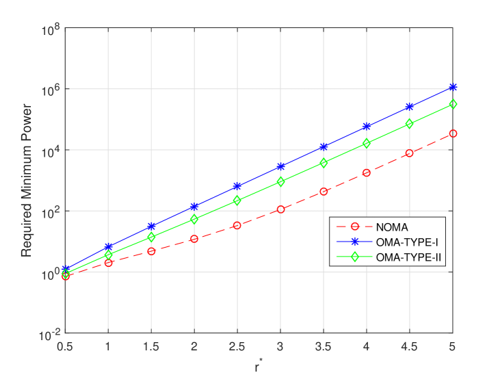
Figure 1: Required minimum power versus $r^{*}$ for $K=3$ users, with $(h_{1},h_{2},h_{3})=(10,5,1).$

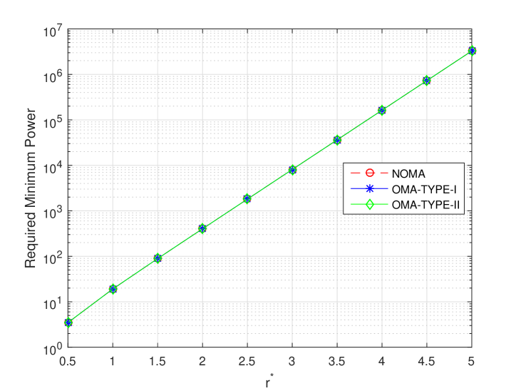
Figure 2: Required minimum power versus $r^{*}$ for $K=3$ users, with $(h_{1},h_{2},h_{3})=(1,1,1).$

Figs. 1 and 2 show the required minimum power versus the target minimum rate $r^{*}$ for different transmission schemes given specified channel realizations. The required minimum power for NOMA, OMA-TYPE-I and OMA-TYPE-II is obtained by the analytical results in (52). In Fig. 1, the channel coefficients are fixed to be $(h_{1},h_{2},h_{3})=(10,5,1)$, and in Fig. 2, the channel coefficients are fixed to be identical, i.e., $(h_{1},h_{2},h_{3})=(1,1,1)$. By observing these two figures, we have the following comments.

1. All the required minimum power of the three systems, i.e., $P_{N}^{*},P_{O1}^{*},P_{O2}^{*}$, increases exponentially as the target minimum rate, i.e., $r^{*}$, increases.

2. When the channel coefficients are not the same, the required minimum power of OMA-TYPE-II is smaller than that of OMA-TYPE-I, while the required minimum power of NOMA is smaller than that of OMA-TYPE-II. Note that these observations are consistent with our analytical results in (53).

3. When the channel coefficients are identical, all the three kinds of required minimum power become the same.

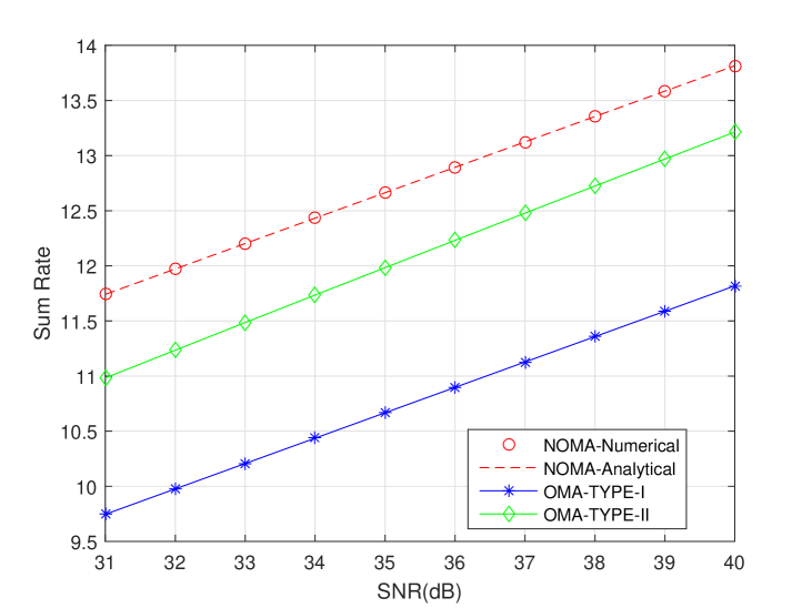
Figure 3: Sum rates versus SNR, with $K=3$, and $(h_{1},h_{2},h_{3},r^{*})=(10,5,1,1)$

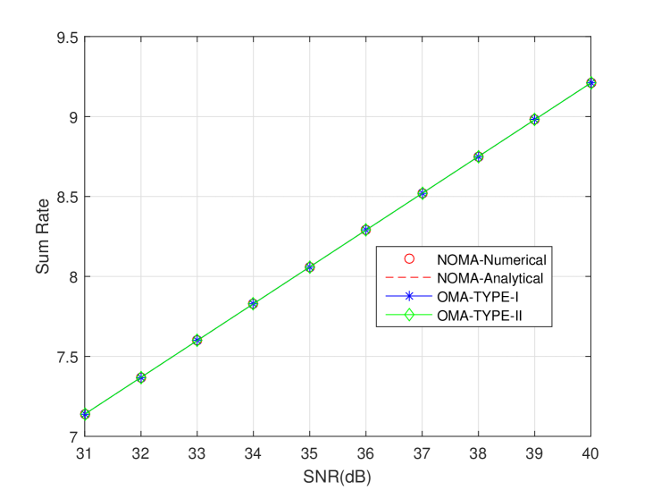
Figure 4: Sum rates versus SNR, with $K=3$, and $(h_{1},h_{2},h_{3},r^{*})=(1,1,1,1)$

Figs. 3 and 4 show the sum rates versus SNR for different transmission schemes given specified channel realizations. The optimum sum rates for NOMA-Numerical, OMA-TYPE-I, and OMA-TYPE-II are obtained by solving the optimization problems in (3), (4) and (6), respectively. The optimum sum rates for NOMA-Analytical are attained by the analytical closed-form expression in (54). In Fig. 3, the channel coefficients are fixed to be $(h_{1},h_{2},h_{3})=(10,5,1)$, and in Fig. 4, the channel coefficients are fixed to be identical, i.e., $(h_{1},h_{2},h_{3})=(1,1,1)$. For both channel setups, we set $r^{*}=1$. By observing these figures, we have the following comments.

1. The numerical and analytical results for NOMA match perfectly.

2. When the channel coefficients are not the same, the sum rates of OMA-TYPE-II are always larger than those of OMA-TYPE-I, while the sum rates of NOMA are always larger than those of OMA-TYPE-II. Note that these observations are also consistent with our analytical results in (55).

3. When the channel coefficients are identical, all the three kinds of sum rates become the same.

IV-B Rayleigh Fading Channels

With randomly generated wireless channels, e.g., Rayleigh fading channels, herein, we introduce two performance evaluation metrics, e.g., outage probability and ergodic sum rate, to evaluate and compare the performance of NOMA, OMA-TYPE-I and OMA-TYPE-II.

Recall that a system is in outage if there exists one user who cannot receive its own messages with the given target minimum rate $r^{*}$ for all the possible resource allocation, i.e., the corresponding optimization problem is infeasible. Mathematically, the outage probabilities of NOMA, OMA-TYPE-I and OMA-TYPE-II can be written as

$$\mathrm{Pr}\{P_{N}^{*}>P\},\quad\mathrm{Pr}\{P_{O1}^{*}>P\},\quad\mathrm{Pr}\{P_{O2}^{*}>P\},$$

respectively, and this criterion will be used in Figs. 5 and 6.

In Figs. 7 and 8, we will use the ergodic sum rate as the criterion to evaluate the performance of NOMA, OMA-TYPE-I and OMA-TYPE-II. These ergodic sum rates can be defined as in the following. Without loss of generality, take NOMA system as an example. Denote $R_{N}(\mathbf{h})$ by the instantaneous optimum sum rate achieved by NOMA and $P_{N}^{*}(\mathbf{h})$ by the required minimum power of NOMA given a specific channel realization $\mathbf{h}=[h_{1},h_{2},...,h_{K}]^{T}$. Note that the instantaneous optimum sum rate reduces to zero if the optimization problem in (3) is infeasible, i.e., the system is in outage. Therefore, the instantaneous optimum sum rate achieved by NOMA can be mathematically expressed as follows:

$$R_{N}(\mathbf{h})=\left\{\begin{aligned} &R_{N}\quad&\text{if}\quad P_{N}^{*}(\mathbf{h})\leq P,\\ &0\quad&\text{Otherwise,}\end{aligned}\right.$$

where $R_{N}$ and $P_{N}^{*}(\mathbf{h})$ are defined in (52) and (54), respectively. With such a definition of the instantaneous optimum sum rate, the ergodic sum rate of NOMA is defined as the expectation of $R_{N}(\mathbf{h})$ with respect to independent and identically distributed (i.i.d.) Rayleigh fading $h_{i}$’s . Note that the ergodic sum rates of OMA-TYPE-I and OMA-TYPE-II can be defined similarly.

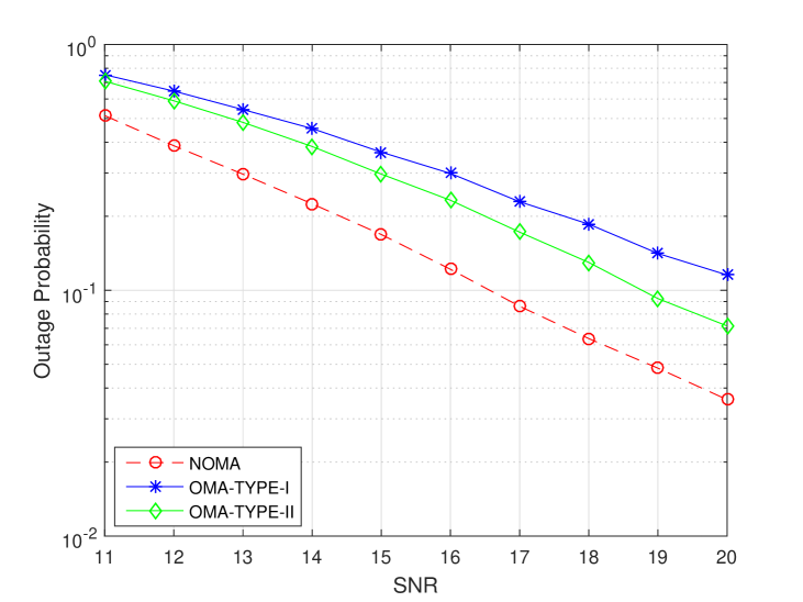
Figure 5: Outage Probability versus SNR, with $K=3,r^{*}=1$

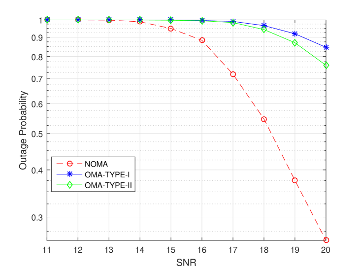
Figure 6: Outage Probability versus SNR, with $K=5,r^{*}=1$

In Figs. 5 and 6, given a fixed target minimum rate $r^{*}=1$, the outage performance versus the SNR for different transmission schemes under Rayleigh fading channels are plotted with $K=3$ and $K=5$, respectively. Since our analytical results show that $P_{N}^{*}\leq P_{O2}^{*}\leq P_{O1}^{*}$, we can infer that

$$\mathrm{Pr}\{P_{N}^{*}>P\}\leq\mathrm{Pr}\{P_{O2}^{*}>P\}\leq\mathrm{Pr}\{P_{O1}^{*}>P\}.$$

This conclusion is confirmed by both Figs. 5 and 6. Particularly, in Fig. 5, OMA-TYPE-II yields about a gain of 1.5dB over OMA-TYPE-I, and NOMA has about a gain of 2.5dB over OMA-TYPE-II at $\mathrm{Pr}=10^{-1}$. Moreover, by comparing Fig. 5 with Fig. 6, it is also observed that the outage probability gain by NOMA becomes larger when the number of users increases.

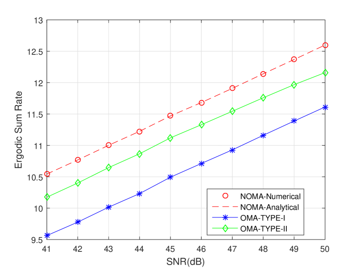
Figure 7: Ergodic Sum Rates versus SNR, with $K=3,r^{*}=1$

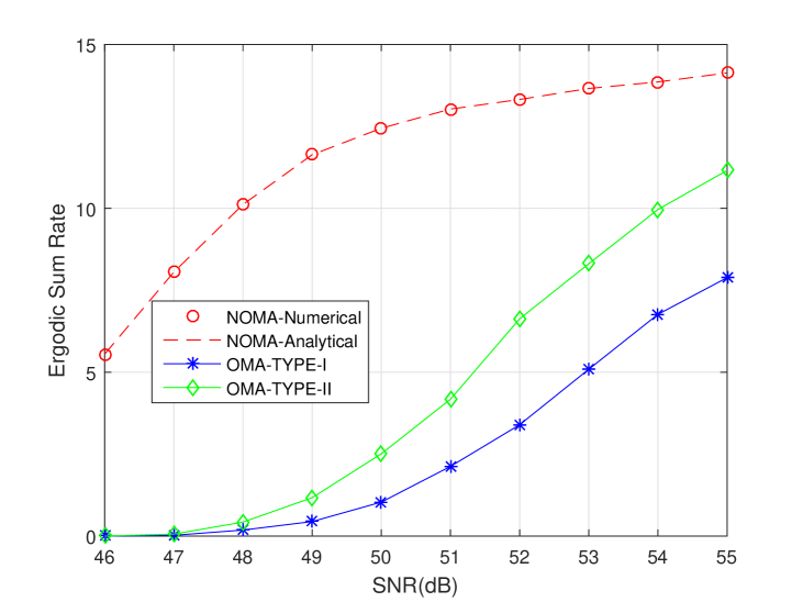
Figure 8: Ergodic Sum Rates versus SNR, with $K=6,r^{*}=2$

In Figs. 7 and 8, the ergodic sum rate performance versus SNR for different transmission schemes under Rayleigh fading channels are plotted with $K=3,r^{*}=1$ and $K=6,r^{*}=2$, respectively. By observing these figures, we have the following comments.

1. The ergodic sum rate of NOMA is always larger than that of OMA-TYPE-II, and the ergodic sum rate of OMA-TYPE-II is always larger than that of OMA-TYPE-I.

2. When the transmission power is large enough with respect to the target minimum rate $r^{*}$, i.e., the outage probabilities for all the three systems tend to zero, the ergodic sum rate increases linearly with SNR. For example, in Fig. 7, NOMA has about a gain of 0.3 nats per channel use (NPCU) over OMA-TYPE-II, and OMA-TYPE-II has about a gain of 0.7 NPCU over OMA-TYPE-I, for all the SNRs.

3. When the transmission power is not large enough with respect to the target minimum rate $r^{*}$, i.e., a system may be in outage, both OMA-TYPE-I and OMA-TYPE-II may suffer a significant performance loss compared to NOMA in the low SNR regime. For example, in Fig. 8, when $\mathrm{SNR}=46\mathrm{dB}$, the ergodic sum rates of OMA-TYPE-I and OMA-TYPE-II decease to nearly zero, while the ergodic sum rate of NOMA can be still maintained over 5 NPCU.

V Conclusion

In this paper, we have mathematically compared the optimum sum rate performance for NOMA and OMA systems, with consideration of user fairness. Firstly, the closed-form optimum sum rate and the corresponding power allocation policy for NOMA systems have been derived, by using the power splitting method. Secondly, the fact that NOMA can always achieve better sum rate performance than that of traditional OMA-TYPE-I with optimum power allocation but equal user time/frequency allocation has been revealed, by a rigorous mathematical proof. Thirdly, we have proved that NOMA can also outperform OMA-TYPE-II with power and time/frequency allocation jointly optimized in terms of sum rate performance. Moreover, the major analytical results have been extracted from those mathematical proofs. Finally, computer simulations have been conducted to validate the correctness of these analytical results and show the advantages of NOMA over OMA in practical Rayleigh fading channels.

References

• [1] Y. Saito, Y. Kishiyama, A. Benjebbour, T. Nakamura, A. Li, and K. Higuchi, “Non-orthogonal multiple access (NOMA) for cellular future radio access,” in Proc. IEEE Vehicular Technology Conference (VTC Spring), Dresden, Germany, Jun. 2013.
• [2] Z. Ding, Z. Yang, P. Fan, and H. V. Poor, “On the performance of non-orthogonal multiple access in 5G systems with randomly deployed users,” IEEE Signal Process. Lett., vol. 21, no. 12, pp. 1501–1505, 2014.
• [3] A. Benjebbour, Y. Saito, Y. Kishiyama, A. Li, A. Harada, and T. Nakamura, “Concept and practical considerations of non-orthogonal multiple access (NOMA) for future radio access,” in Proc. IEEE International Symposium On Intelligent Signal Processing and Communications Systems (ISPACS), 2013, pp. 770–774.
• [4] Study on downlink multiuser superposition transmission for LTE, 3rd Generation Partnership Project (3GPP) Std., Mar. 2015.
• [5] Q. C. Li, H. Niu, A. T. Papathanassiou, and G. Wu, “5G network capacity: key elements and technologies,” IEEE Veh. Technol. Mag., vol. 9, no. 1, pp. 71–78, 2014.
• [6] L. Dai, B. Wang, Y. Yuan, S. Han, I. Chih Lin, and Z. Wang, “Non-orthogonal multiple access for 5G: solutions, challenges, opportunities, and future research trends,” IEEE Commun. Mag., vol. 53, no. 9, pp. 74–81, 2015.
• [7] T. M. Cover and J. A. Thomas, Elements of information theory.   New York, NY, USA: John Wiley & Sons, 2012.
• [8] D. Tse and P. Viswanath, Fundamentals of wireless communication.   New York, NY, USA: Cambridge university press, 2005.
• [9] Z. Ding, M. Peng, and H. V. Poor, “Cooperative non-orthogonal multiple access in 5G systems,” IEEE Commun. Lett., vol. 19, no. 8, pp. 1462–1465, Aug. 2015.
• [10] Z. Ding, P. Fan, and V. Poor, “Impact of user pairing on 5G non-orthogonal multiple access downlink transmissions,” IEEE Trans. Veh. Technol., vol. 65, no. 8, pp. 6010–6023, Aug. 2016.
• [11] P. Xu, Z. Ding, X. Dai, and H. V. Poor, “A new evaluation criterion for non-orthogonal multiple access in 5G software defined networks,” IEEE Access, vol. 3, pp. 1633–1639, 2015.
• [12] Z. Ding, F. Adachi, and H. V. Poor, “The application of MIMO to non-orthogonal multiple access,” IEEE Trans. Wireless Commun., vol. 15, no. 1, pp. 537–552, Jan. 2016.
• [13] Z. Ding, R. Schober, and H. V. Poor, “A general MIMO framework for NOMA downlink and uplink transmission based on signal alignment,” IEEE Trans. Wireless Commun., vol. 15, no. 6, pp. 4438–4454, Jun. 2016.
• [14] Z. Chen, Z. Ding, P. Xu, and X. Dai, “Optimal precoding for a QoS optimization problem in two-user MISO-NOMA downlink,” IEEE Commun. Lett., vol. 20, no. 6, pp. 1263–1266, Jun. 2016.
• [15] Z. Chen, Z. Ding, X. Dai, and G. Karagiannidis, “On the application of quasi-degradation to MISO-NOMA downlink,” IEEE Trans. Signal Process., vol. 64, no. 23, pp. 6174–6189, Dec. 2016.
• [16] Z. Chen, Z. Ding, and X. Dai, “Beamforming for combating inter-cluster and intra-cluster interference in hybrid NOMA systems,” IEEE Access, vol. 4, pp. 4452–4463, 2016.
• [17] Z. Chen and X. Dai, “MED precoding for multi-user MIMO-NOMA downlink transmission,” IEEE Trans. Veh. Technol., to be published, 2016.
• [18] N. Jindal and A. Goldsmith, “Capacity and optimal power allocation for fading broadcast channels with minimum rates,” IEEE Trans. Inf. Theory, vol. 49, no. 11, pp. 2895–2909, 2003.
• [19] S. Boyd and L. Vandenberghe, Convex optimization.   New York, NY, USA: Cambridge university press, 2004.