Peer Prediction with Heterogeneous Tasks

Abstract

Peer prediction promotes contributions of useful information by users in settings in which there is no way to verify the quality of responses. This paper introduces the problem of peer prediction with heterogeneous tasks, where each task is associated with a different distribution on responses. The motivation comes from eliciting user-generated content about places in a city, where tasks vary because places and questions about places vary. We extend the correlated agreement (CA) mechanism ((?)) to this setting, aligning incentives for investing effort without creating opportunities for coordinated manipulations. We demonstrate in simulation much better incentive properties than other mechanisms, using data from user reports on a crowdsourcing platform.

1 Introduction

Peer prediction refers to the problem of scoring information reports in settings where the correctness of a report cannot be verified, either because there is no objectively correct answer or because this answer is too costly to acquire. This problem arises in diverse contexts; e.g., peer assessment of assignments in massive open online courses, and when collecting feedback about a new restaurant. Peer prediction algorithms use reports from multiple participants to score contributions.

Simple approaches compare the responses of two users and award them if they agree. But this does not promote truthful reporting when one user believes that it is unlikely that another user will have the same opinion. This problem can be alleviated by adjusting scores according to the frequency of reports (?; ?; ?).

A limitation of current approaches, however, is that tasks are assumed to be ex ante identical, with each task associated with the same distribution on reports. But tasks on various maps platforms, which seek to elicit content from users about places in a city, are quite heterogeneous. On this kind of platform, a user is encouraged to answer several different types of questions (= tasks) related to the same place; e.g., “is the restaurant noisy?,” “is it accessible by wheelchair?,” or “does it serve wine?” The questions are related to the same place, yet the prior beliefs about the distribution on reports for each type of question may be very different.

We design a new, multi-task peer prediction mechanism (the correlated agreement-heterogeneous mechanism) that is responsive to this challenge. This new mechanism shares similar properties with the earlier correlated agreement (CA) mechanism (?). In particular, it is informed truthful under weak conditions, meaning that it is strictly beneficial for a user to invest effort and acquire information, and that truthful reporting is the best strategy when investing effort, as well as an equilibrium. We demonstrate that the mechanism has good incentive properties when tested in simulation on distributions derived from user reports on a popular maps platform.

1.1 Related Work

We focus in this brief discussion on mechanisms that are minimal, in the sense that they only require signal (or information) reports and do not require belief reports. Miller et al. ? introduced the peer prediction problem and proposed a minimal mechanism that has truthful reporting in an equilibrium, however the mechanism’s design requires knowledge of the joint signal distribution and is vulnerable to coordinated misreports. In response, Jurca and Faltings (?) show how to eliminate uninformative, pure-strategy equilibria through a three-peer mechanism, and Kong et al. (?) provide a method to design robust, single-task, binary signal mechanisms.

Witkowski and Parkes (?) first introduced the combination of learning and peer prediction, coupling the estimation of the signal prior together with the shadowing mechanism. There has also been work on making use of reports from a large population and coupling scoring with estimation. For a setting with latent ground truth model, Kamble et al. (?) provide mechanisms that guarantee strict incentive compatibility with a large number of agents. Radanovic et al. (?) provide a mechanism in which truthfulness is the highest-paying equilibrium in the asymptote of a large population and with a self-predicting condition that places a structure on the correlation structure.

Dasgupta and Ghosh (?) show that robustness to coordinated misreports can be achieved by using reports across multiple tasks along with access to partial information about the joint distribution. The main insight in the DG mechanism is to reward agents if they provide the same signal on the same task, but punish them if one agent’s report on one task is the same as another’s on another task. Shnayder et al. (?) generalize DG to handle multiple signals, and show how the required knowledge about the distribution (the correlation structure on pairs of signals) can be estimated from reports without compromising incentives. Their correlated agreement (CA) mechanism rewards pairs of reports on the same task (penalizes pairs of reports on different tasks) based on whether signals are positively or negatively correlated. On the other hand,  (?) generalize the CA mechanism when users are heterogeneous and derive sample complexity bounds for learning the reward matrices. Shnayder et al. (?) adopt replicator dynamics as a model of population learning in peer prediction, and confirm that these multi-task mechanisms (including Kamble et al. (?)) are successful at avoiding uninformed equilibria.

To the best of our knowledge, there is no prior work on extending the design of these multiple-task mechanisms to heterogeneous tasks, where pairs of reports may be on different types of tasks, with each task associated with a different signal distribution.

2 Heterogeneous, Multi-Task Peer Prediction

Consider two agents, $1$ and $2$, who are members of a large population. Each agent is assigned to a set of $M=\{1,2,\ldots,m\}$ tasks. We adopt a binary effort model: if an agent invests effort he incurs a cost and obtains an informed signal, otherwise the agent receives no signal. There are $n$ signals. We do not assume that tasks are ex ante identical, however, we do assume that the signals for different tasks are drawn independently.

Let $S^{1}_{k}$ and $S^{2}_{k}$ respectively be the signals of agents $1$ and $2$ for task $k$ (if investing effort). Let $P_{k}(i,j)=\mathrm{Pr}\left(S^{1}_{k}=i,S^{2}_{k}=j\right)$ be the joint probability for a pair of signals $(i,j)$ on task $k$ and let $P_{k}(i)$ and $P_{k}(j)$ be the corresponding marginal probabilities. We assume that the agents are exchangeable in their roles in these distributions, with the same marginal distributions and joint distributions for any pair of agents.

An agent’s strategy maps every task and every received signal to a reported signal. Agents make reports without knowledge of each others’ reports. We assume that the type of task, and signal about a task (upon investing effort), is the only information available to an agent. For the theoretical analysis, we assume that an agent adopts the same strategy across all tasks. We leave the analysis of asymmetric strategies for future work. We allow an agent’s strategy to be randomized, i.e. a probability distribution over the set of possible signals. We will write $F$ and $G$ to denote the mixed strategies of agents $1$ and $2$ respectively. Let $\mathbb{I}$ denote the truthful strategy i.e. $\mathbb{I}(j)=j$. As in  Shnayder et al. (?), we are interested in the following two incentive properties:

Definition 2.1.

(Strong Truthful) A peer prediction mechanism is strong truthful iff for all strategies $F,G$ we have $E(\mathbb{I},\mathbb{I})\geq E(F,G)$, where equality may hold only when $F$ and $G$ are both the same permutation strategy (i.e. a bijection from received signals to reported signals.)

Definition 2.2.

(Informed Truthful) A peer prediction mechanism is informed truthful iff for all strategies $F,G$ we have $E(\mathbb{I},\mathbb{I})\geq E(F,G)$, where equality may hold only when $F$ and $G$ are informed strategies (i.e. reports depend on an agent’s signal).

These two truthfulness properties imply that truthful reporting is a strict and weak correlated equilibrium, respectively (?). They also ensure that there are no useful, coordinated misreports available to agents.

2.1 Delta Matrices

Following Shnayder et al. (?) to multiple types of tasks, a first approach would be to define the following $n\times n$ matrix for task $k$:

$$\Delta_{k}(i,j)=P_{k}(i,j)-P_{k}(i)P_{k}(j).$$ (1)

Let $S_{k}$ be the sign matrix of $\Delta_{k}$ i.e. $S_{k}(i,j)=1$ if $\Delta_{k}(i,j)>0$ and $S_{k}(i,j)=0$ otherwise.

In the original CA mechanism (?), each task $k$ is ex ante identical, and thus has the same delta matrix. Denote this matrix $\Delta$, with $S$ the corresponding sign matrix. The original CA mechanism works as follows:

1. Let $r^{1}_{k}$ ($r^{2}_{k}$) be the signal reported by agent $1$ ($2$) on task $k$.

2. Pick a task $b$ uniformly at random as the bonus task, and pick penalty tasks $l^{\prime}$ and $l^{\prime\prime}$ (with $l^{\prime}\neq l^{\prime\prime}$) uniformly at random from the remaining tasks.

3. Pay each agent $S(r^{1}_{b},r^{2}_{b})-S(r^{1}_{l^{\prime}},r^{2}_{l^{\prime\prime}})$.

A simple generalization is to pay $S_{b}(r^{1}_{b},r^{2}_{b})-S_{b}(r^{1}_{l^{\prime}},r^{2}_{l^{\prime\prime}})$, where $S_{b}$ is the sign matrix corresponding to the bonus task. But this is not informed truthful for heterogeneous tasks. This is demonstrated in Example 1.

Example 1 (CA is not informed truthful with heterogeneous tasks).

Consider three tasks (1, 2 and 3) with the following joint probability distributions

$$\begin{array}[]{cc@{}c@{}c}&\begin{array}[]{cc}Y&N\end{array}&\begin{array}[]{cc}Y&N\end{array}&\begin{array}[]{cc}Y&N\end{array}\\ \begin{array}[]{c}Y\\ N\end{array}&\left[\begin{array}[]{cc}0.4&0.22\\ 0.22&0.16\\ \end{array}\right]&\left[\begin{array}[]{cc}0.7&0.14\\ 0.14&0.02\\ \end{array}\right]&\left[\begin{array}[]{cc}0.4&0.22\\ 0.22&0.16\\ \end{array}\right]\\ &(P_{1})&(P_{2})&(P_{3})\end{array}$$

and the following sign matrices:

$$\mathit{sign}(\Delta_{1}):\begin{bmatrix}1&0\\ 0&1\end{bmatrix}\ \mathit{sign}(\Delta_{2}):\begin{bmatrix}0&1\\ 1&0\end{bmatrix}\ \mathit{sign}(\Delta_{3}):\begin{bmatrix}1&0\\ 0&1\end{bmatrix}$$

Suppose each agent adopts the truthful strategy, and task 1 is the bonus task, and 2 and 3 are the penalty tasks for agents 1 and 2, respectively. Then the expected score is

$$\sum_{i,j}P_{1}(i,j)S_{1}(i,j)-P_{2}(i)P_{3}(j)S_{1}(i,j),$$

which evaluates to $-0.0216$. This is true irrespective of whether the penalty tasks for 1 and 2, respectively, are 2 and 3 or 3 and 2. Similarly, we can show that the expected scores are $-0.1912$ and $-0.0216$ when the bonus task is task $2$ and $3$, respectively.

Now consider the case when the first agent always reports $N$. Suppose task $1$ is the bonus task and tasks $2$ and $3$ are the penalty tasks for 1 and 2, respectively. The expected score is

$$\sum_{i,j}P_{1}(i,j)S_{1}(N,j)-P_{2}(i)P_{3}(j)S_{1}(N,j),$$

which evaluates to $0$. Similarly, for task 3 and 2 as the penalty for 1 and 2, respectively, the expected score is $0.22$. So on average, the expected score for task 1 as bonus is $0.11$. Similar calculations show expected scores of 0.22 and 0.11, for tasks 2 and 3 as bonus, respectively. Thus, the CA mechanism fails to be informed truthful for this example.

3 The Correlated-Agreement Heterogeneous (CAH) Mechanism

In this section, we extend the CA mechanism to handle heterogeneous tasks. The main idea is to modify the delta matrix for a bonus task to allow for the implied product distribution on signals on penalty tasks. Algorithm 1 describes the CAH mechanism.

Algorithm 1 CAH mechanism

1:Joint probability distribution $P_{b}(\cdot,\cdot)$, marginal probability distributions $\{P_{l}(\cdot)\}_{l\neq b}$ and reports $\{r^{1}_{k},r^{2}_{k}\}_{k=1}^{m}$

2:$b\leftarrow$ uniformly at random from $\{1,\ldots,m\}$ (bonus task)

3:$l^{\prime}\leftarrow$ uniformly at random from $\{1,\ldots,m\}\setminus\{b\}$ (penalty task assigned to agent 1)

4:$l^{\prime\prime}\leftarrow$ uniformly at random from $\{1,\ldots,m\}\setminus\{b,l^{\prime}\}$ (penalty task assigned to agent 2)

5:Define $\Delta_{b}(i,j)$ as

$$\!\!\!\!P_{b}(i,j)-\frac{1}{(m-1)(m-2)}\!\sum_{\stackrel{{\scriptstyle t^{\prime},t^{\prime\prime}\in[m]\setminus\{b\}}}{{\&\ t^{\prime}\neq t^{\prime\prime}}}}\!\!\!\!P_{t^{\prime}}(i)P_{t^{\prime\prime}}(j)$$ (2)

6:Let $S_{b}(i,j)$ be the corresponding score matrix i.e.

$$S_{b}(i,j)=1\text{ if }\Delta_{b}(i,j)>0\text{ and }S_{b}(i,j)=0\ \text{otherwise}$$

7:Make payment $S_{b}(r^{1}_{b},r^{2}_{b})-S_{b}(r^{1}_{l^{\prime}},r^{2}_{l^{\prime\prime}})$ to each agent

In analyzing the properties of CAH, we note that it is sufficient to consider only deterministic strategies. The proof of this statement is analogous to Lemma 3.2 (?), and uses the fact that the maximization of a linear function over a convex region is extremal.

Given this, let $F_{i}$ ($G_{j}$) denote the report of agents 1 (2) on signal $i$ ($j$). The expected score for strategies $F$ and $G$, conditioned on some bonus task $b$, denoted as $E_{b}(F,G)$, is:

$$\mathbf{E}_{l^{\prime},l^{\prime\prime}}\left[\sum_{i,j}P_{b}(i,j)S_{b}(F_{i},G_{j})-\sum_{i,j}P_{l^{\prime}}(i)P_{l^{\prime\prime}}(j)\right]$$

$$=\sum_{i,j}P_{b}(i,j)S_{b}(F_{i},G_{j})$$

$$-\sum_{\stackrel{{\scriptstyle l^{\prime},l^{\prime\prime}\in[m]\setminus\{b\}}}{{\&\ l^{\prime}\neq l^{\prime\prime}}}}\frac{1}{(m-1)(m-2)}\sum_{i,j}P_{l^{\prime}}(i)P_{l^{\prime\prime}}(j)S_{b}(F_{i},G_{j})$$

$$=\sum_{i,j}\Delta_{b}(i,j)S_{b}(F_{i},G_{j}),$$ (3)

where $\ell$ and $\ell^{\prime\prime}$ denote agent 1 and agent 2’s penalty tasks, respectively. Thus, the expected score, averaged over the $m$ possible bonus tasks, is

$$E(F,G)=\frac{1}{m}\sum_{b=1}^{m}E_{b}(F,G)=\frac{1}{m}\sum_{b=1}^{m}\sum_{i,j}\Delta_{b}(i,j)S_{b}(F_{i},G_{j})$$ (4)

We now state a property about the delta matrices (2).

Lemma 1.

For each task $b$, we have $\sum_{i,j}\Delta_{b}(i,j)=0$

Proof.

See Appendix 6.1 ∎

3.1 Informed Truthfulness

The CAH mechanism is informed truthful under a weak condition on the signal distributions.

Theorem 2.

If for each task $b$, $\Delta_{b}$ is symmetric and each entry of $\Delta_{b}$ is non-zero, then the CAH mechanism is informed truthful.

Proof.

For any bonus task $b$, the truthful strategy $(\mathbb{I},\mathbb{I})$ has higher expected score than any other pair of strategies $F,G$:

$$E_{b}(\mathbb{I},\mathbb{I})=\sum_{i,j}\Delta_{b}(i,j)S_{b}(i,j)=\sum_{i}\sum_{j}\max(0,\Delta_{b}(i,j))$$

$$\geq\sum_{i,j}\Delta_{b}(i,j)S_{b}(F_{i},G_{j})=E(F,G).$$

Consider an uninformed strategy $F$, with $F_{i}=r$ for all $i$. Then for any $G$, the expected score is

$$\sum_{i=1}^{n}\sum_{j=1}^{n}\Delta_{b}(i,j)S_{b}(r,G_{j})=\sum_{j=1}^{n}S_{b}(r,G_{j})\sum_{i=1}^{n}\Delta_{b}(i,j)$$

$$\leq\sum_{j=1}^{n}\max(0,\sum_{i=1}^{n}\Delta_{b}(i,j)).$$

We need to show the following:

$$\sum_{j=1}^{n}\max(0,\sum_{i=1}^{n}\Delta_{b}(i,j))<\sum_{j=1}^{n}\sum_{i=1}^{n}\max(0,\Delta_{b}(i,j)).$$

It is enough to show that for each $b$, there exists a column $j$ and two different rows $i_{1},i_{2}$ such that $\Delta_{b}(i_{1},j)>0$ and $\Delta_{b}(i_{2},j)<0$. Suppose not. Then each column of $\Delta_{b}$ has either all positive entries or all negative entries. Since each entry of $\Delta_{b}$ is non-zero and Lemma 1 holds, there exist two columns $j_{1}$ and $j_{2}$ such that all entries of $j_{1}$ ($j_{2}$) are positive (negative). This implies $\Delta_{b}(j_{2},j_{1})>0$ and $\Delta_{b}(j_{1},j_{2})<0$, which contradicts the fact that $\Delta_{b}$ is symmetric. ∎

3.2 Strong Truthfulness

We state a sufficient condition for the CAH mechanism to satisfy the property of strong truthfulness.

Condition 1 :

1. $\Delta_{b}(i,i)>0$, $\quad\forall b\ \forall i$.

2. $\sum_{b=1}^{m}\Delta_{b}(i,j)<0$, $\quad\forall i\neq j$.

Theorem 3.

If $\{\Delta_{b}\}_{b=1}^{m}$ satisfy Condition 1, then the CAH mechanism is strongly truthful.

Proof.

See Appendix 6.2. ∎

Condition 1 is slightly weaker than the categorical condition (?). $\Delta_{b}$ is categorical if (1) $\Delta_{b}(i,i)>0$ for all signals $i$, and (2) $\Delta_{b}(i,j)<0$ whenever $i\neq j$; i.e., same-signal positive correlation and other-signal negative correlation. Condition 1 does not require every off-diagonal entry to be negative for all tasks $b$, but only that the average of the off-diagonal entries is negative. Categorical and Condition 1 are equivalent when there are only two signals.

3.3 Combining CAH with Estimation

As with the CA mechanism (?), the CAH mechanism remains (approximately) informed truthful even when the statistics used to determine scores are estimated from the reports of strategic agents. The reason is that the score matrix that corresponds to the correct statistics is the best possible score matrix for agents, and thus they cannot do better by cooperating in designing an alternate matrix.

(Algorithm 2) presents the detail-free version of CAH mechanism, which learns the delta matrices from the agents’ reports. We will refer to this implementation as CAHR (in short for CAH recomputed). The next theorem proves that CAHR is $(\varepsilon,\delta)$-informed truthful.

Theorem 4.

If there are at least $q=\Omega\left(\frac{n}{\varepsilon^{2}}\log\left(\frac{m}{\delta}\right)\right)$ agents reviewing each task, for $m$ tasks and $n$ possible signals, then with probability at least $1-\delta$, then CAHR satisfies

$$E\left[\mathbb{I},\mathbb{I}\right]\geq E\left[F,G\right]-\varepsilon\quad\forall F,G$$

Proof.

See Appendix 6.3 ∎

Theorem 4 implies that truthful reporting is an approximate equilibrium for the detail-free CAH, and that (up to $\epsilon$) there is no useful joint deviation. The proof follows from the fact that any joint distribution $P_{b}(\cdot,\cdot)$ (resp. marginal distribution $P_{b}(\cdot)$) can be learned with $\tilde{O}\left(n^{2}/\varepsilon^{2}\right)$ (resp. $\tilde{O}\left(n/\varepsilon^{2}\right)$) samples and observing that $q$ samples from a task gives us $q^{2}$ samples from the corresponding joint distribution. In addition, we can show a general version of Theorem 4. Suppose there are $t$ distinct types of tasks, and the number of tasks of type $k$ is $m_{k}$. Then it is sufficient to have $q=\tilde{\Omega}\left(\frac{1}{\sqrt{m_{k}}}\frac{n}{\varepsilon^{2}}\right)$ samples from each task of type $k$. This follows from the observation that if we have at least $q$ samples from each task of type $k$ then the total number of samples from the joint distribution $P_{k}(\cdot,\cdot)$ is at least $m_{k}q^{2}=\tilde{\Omega}\left({n^{2}}/{\varepsilon^{2}}\right)$.

Algorithm 2 CAHR mechanism

1:Agent $p$ of a population of $q$ agents provides reviews $(r^{p}_{1},\ldots,r^{p}_{m})$ on each of the $m$ tasks.

2:$T_{k}(i,j)\leftarrow$ observed freq of signal pair $i,j$ on task $k$.

3:Pair up the agents uniformly at random, and run CAH for each pair with the estimated distribution $\{T_{k}(\cdot,\cdot)\}_{k=1}^{m}$

3.4 Cross Correlated Agreement

So far we have assumed that the probabilities of observing signals are independent across different tasks. However, two users’ responses to two different tasks may be correlated (e.g. consider two questions – (1) does this restaurant serve alcohol and (2) does this restaurant serve wine?) We will write $P_{l^{\prime},l^{\prime\prime}}(i,j)$ to denote the probability that a user sees signal $i$ on task $l^{\prime}$ and another user observes signal $j$ on task $l^{\prime\prime}$. When there are no correlations among signals for different questions we have $P_{l^{\prime},l^{\prime\prime}}(i,j)=P_{l^{\prime}}(i)P_{l^{\prime\prime}}(j)$. The Cross Correlated Agreement for Heterogeneous Tasks (CCAH) mechanism generalizes CAH by using the probabilities $P_{l^{\prime},l^{\prime\prime}}(\cdot,\cdot)$ for different pairs of tasks $(l^{\prime},l^{\prime\prime})$.

• CCAH is same as CAH except it defines $\Delta_{b}(i,j)$, the $(i,j)$-th entry of delta matrix for task $b$ as :

  $$P_{b}(i,j)-\frac{1}{(m-1)(m-2)}\sum_{\stackrel{{\scriptstyle t^{\prime},t^{\prime\prime}\in[m]\setminus\{b\}}}{{\&\ t^{\prime}\neq t^{\prime\prime}}}}P_{t^{\prime},t^{\prime\prime}}(i,j)$$

CCAH is strong truthful and informed truthful under similar conditions stated in theorems 3 and 2 respectively. Moreover, a sample complexity result analogous to Theorem 4 holds for a detail-free implementation of CCAH. This is because if we have at least $q$ samples from both $l^{\prime}$ and $l^{\prime\prime}$, then we have at least $q^{2}$ samples from the joint distribution $P_{l^{\prime},l^{\prime\prime}}(\cdot,\cdot)$.

4 Experimental Results

XYZ is a platform for collecting user generated content in regard to places on a mapping platform. A user can provide information by answering ‘yes’, ‘no,’ or ‘not sure’ to a series of questions. A user is awarded one point for each contribution, where a contribution can be a review or a photograph or any update about the place, with a maximum of five points per place. Based on the number of points received a user is in one of five levels on the platform, with higher levels providing better benefits such as free online storage, visibility on the XYZ channel, and access to new products before they are generally released.

A type of task is specified by a triple of the form:

$$\mathit{Region}\times\mathit{BusinessType}\times\mathit{Question}$$

A region is a US state, there are four business types such as “restaurant,” “bar,” “public location” or “cafe” (these are anonymized in our data), and there are 143 distinct questions in the data. The questions are also anonymized, but categorized by XYZ as “subjective” or “factual” (e.g., “is this restaurant noisy?” vs “does this cafe have free WiFi?”). Each task type has a corresponding pairwise signal distribution.

The data are counts of pairs of signal reports, broken down by (region, business type, question). The number of different questions (and thus types of tasks) per pair of region and business type varies from 75 to 135, with an average of 102. There are 51 regions and 4 business types per state. Thus, the total number of task types for which we have data is around 20,885.

For the purpose of our simulations we treat the distributions for these task types as describing the true signal distributions. The goal of the experiments is to compare, under this assumption, the robustness of the CAH mechanism with other mechanisms in the literature. For this, we consider the robust peer truth serum (RPTS) mechanism (?) (which sets a score of $1/P(i)$ for agreement on signal $i$ and $1$ otherwise) and the Kamble (?) mechanism (which sets a score of $1/\sqrt{P(i,i)}$ for agreement on signal $i$).

In simulating CAH, we first compute the delta matrices for each task type using Equation 2. For this, we assume for a given (region, business type, question) that the penalty tasks are sampled from other questions associated with the same (region, business type). From these delta matrices, we then use Equation 3 to compute the expected score for each question, before averaging these scores over all questions associated with a (region, business type) pair. For the single task, RPTS and Kamble mechanisms, we compute the score for a (region, business type) by averaging the individual scores recevied on each question associated with the (region, business type) pair. Finally, since the payments of CAH are bounded between $0$ and $1$, we normalize the payments of RPTS and Kamble to $[0,1]$. Along with CAH, we also evaluate CAHR, the empirical version of the CAH mechanism. CAH has access to the true delta matrices, whereas, CAHR computes the delta matrices based on the reports of the agents and then uses these delta matrices to score reports.

4.1 Unilateral Incentives for Truthful Reports

We consider three kinds of strategic behaviors: constant-0 (report ‘yes’ all the time), constant-1 (report ‘no’ all the time) and random (report ‘yes’ w.p. 0.5).

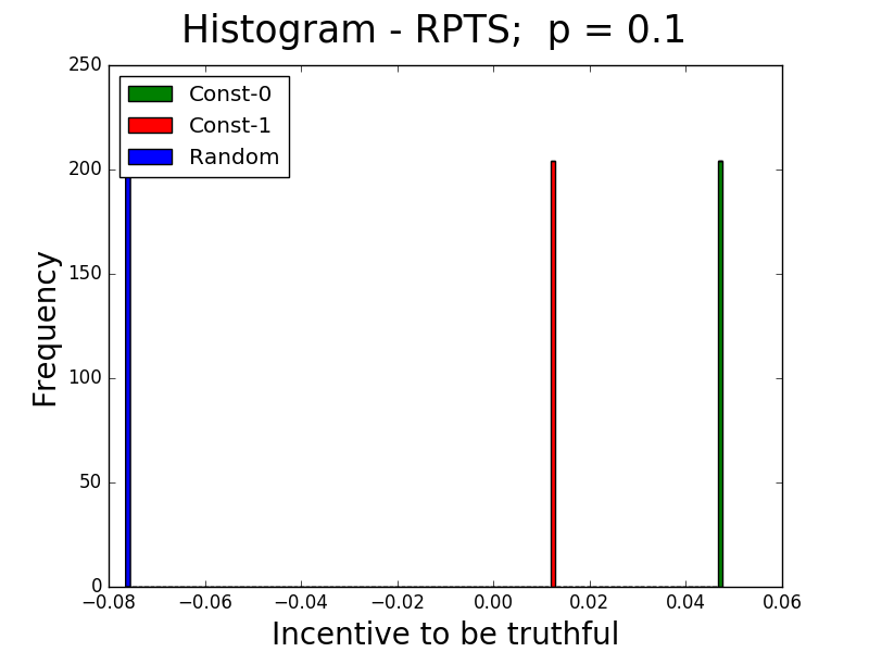
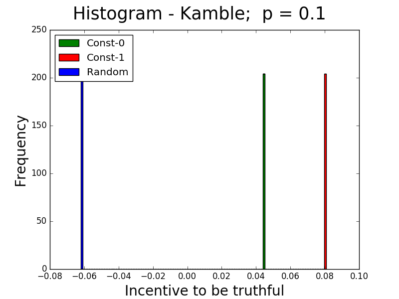
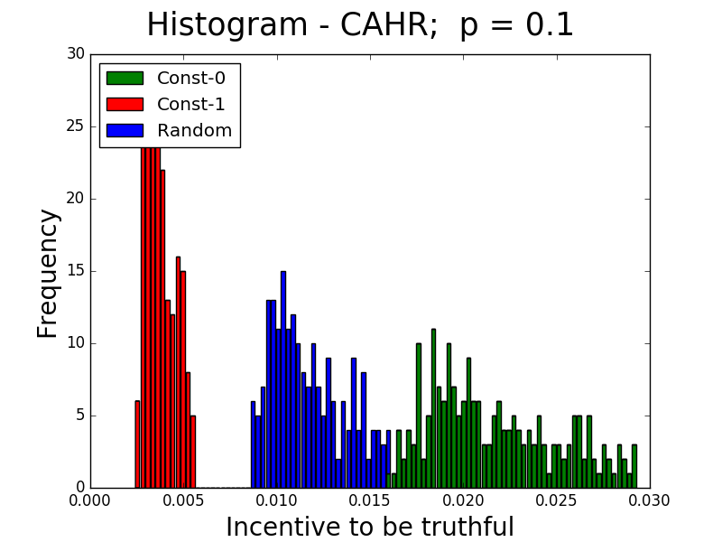
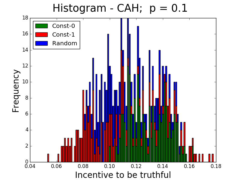
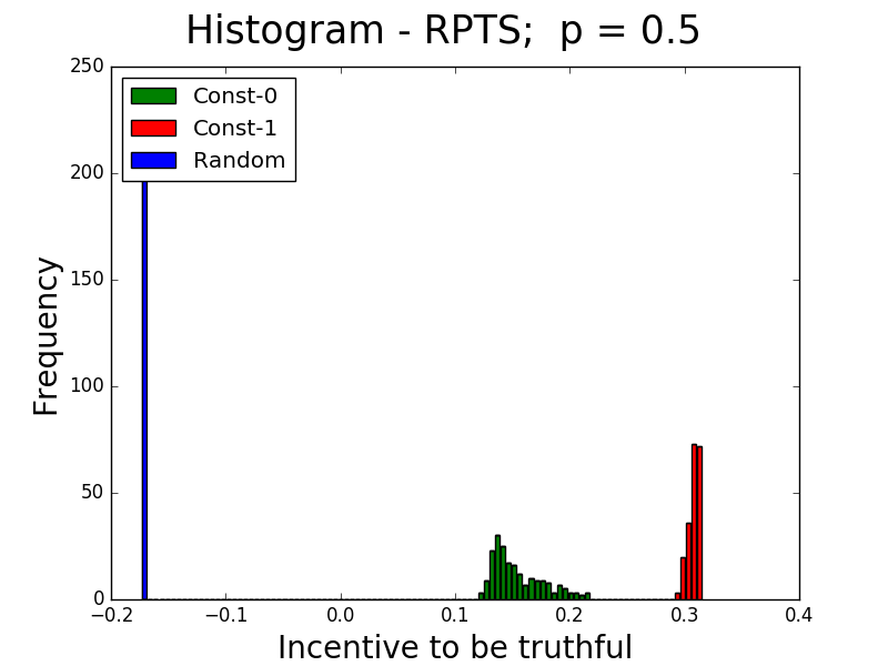
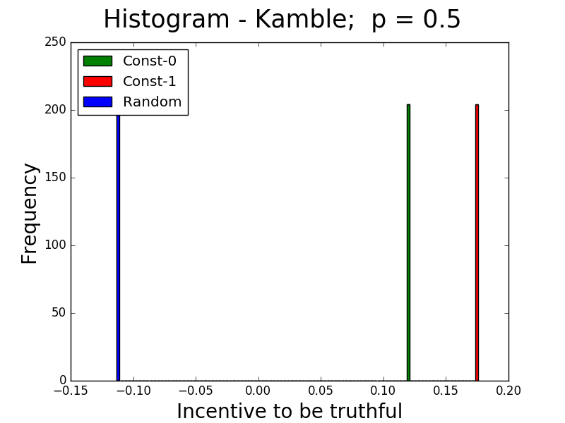
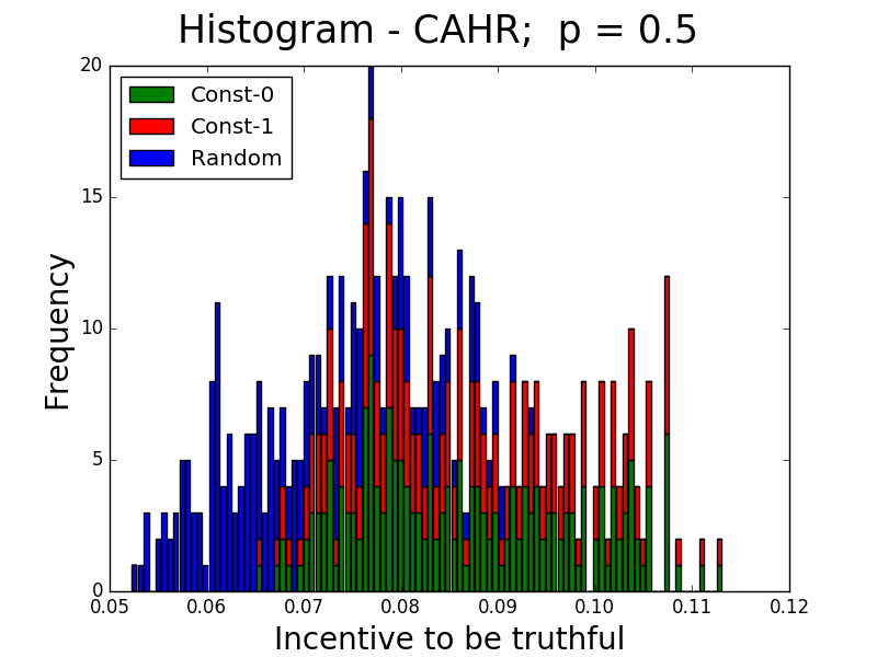
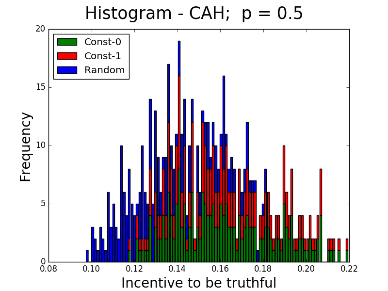
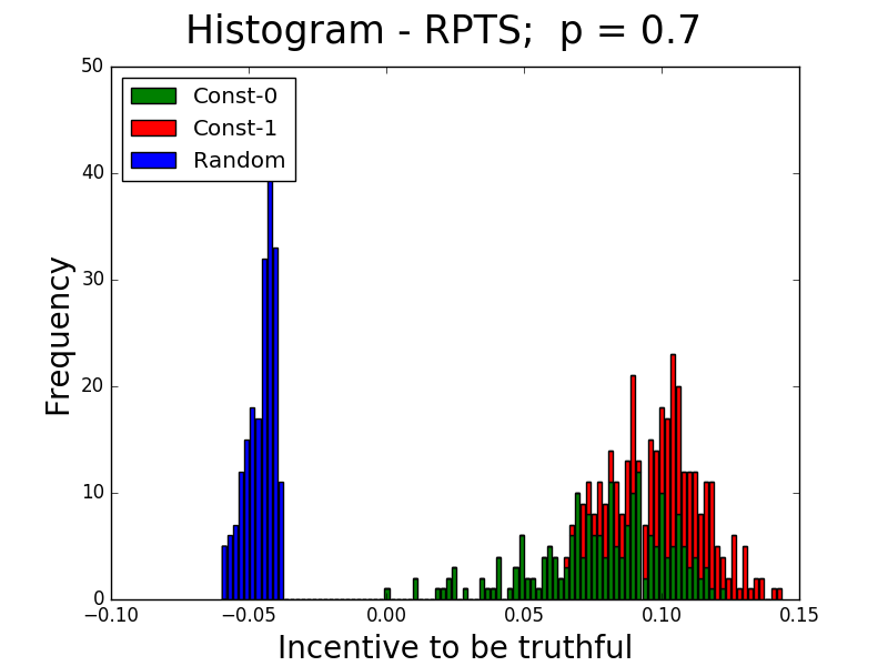
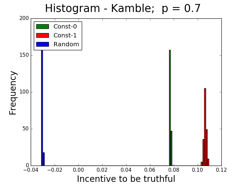
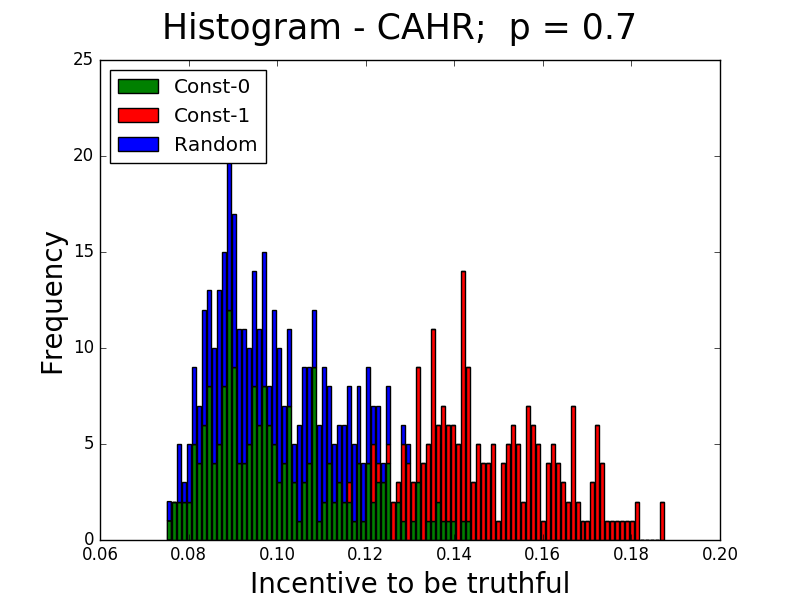
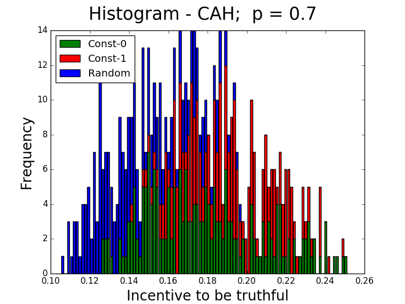
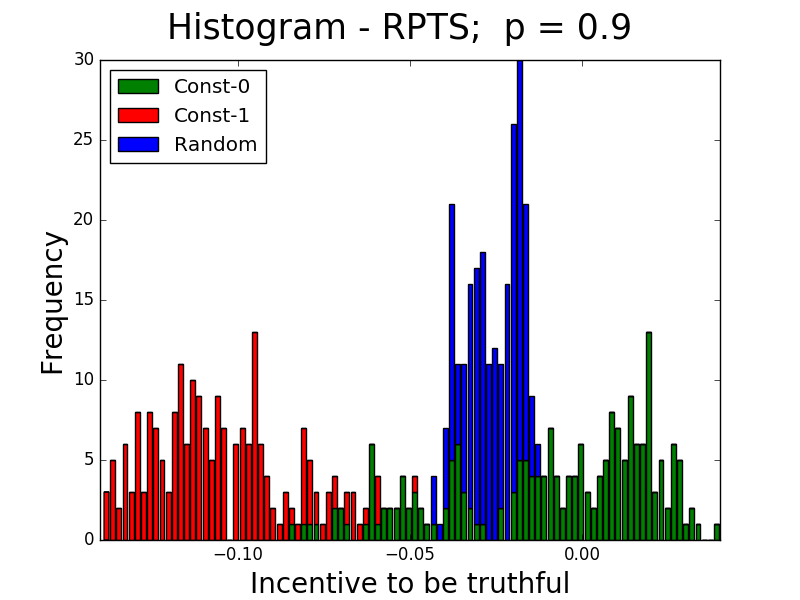
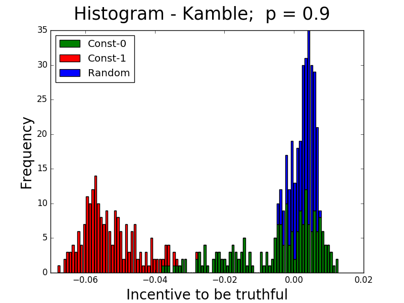
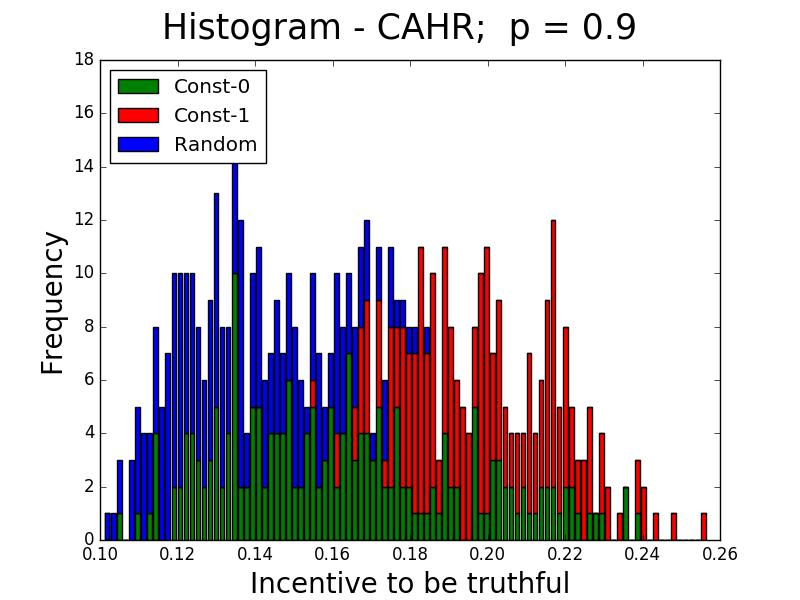
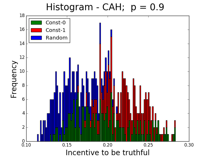
Figure 4: Histograms for the 204 (region, business type) pairs of expected benefit (averaged across questions) from truthful behavior vs. some other strategy, when fraction $p$ is truthful and fraction $1-p$ adopt the same, non-truthful strategy for $p=0.1,0.5,0.7,0.9$

We first consider unilateral incentives to make truthful reports, for various assumptions about how the behavior of the rest of the population. As an illustration, Figure 4 shows the expected benefit to being truthful vs following some other behavior, considering the average score for each (region, business type). We consider, in particular, the benefit to being truthful vs the alternate behavior when $p=0.8$ of the population is truthful and the rest follow the same, alternate strategy. This models 20% of the agents being able to coordinate on a deviation from truthful play.

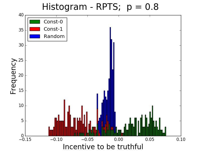
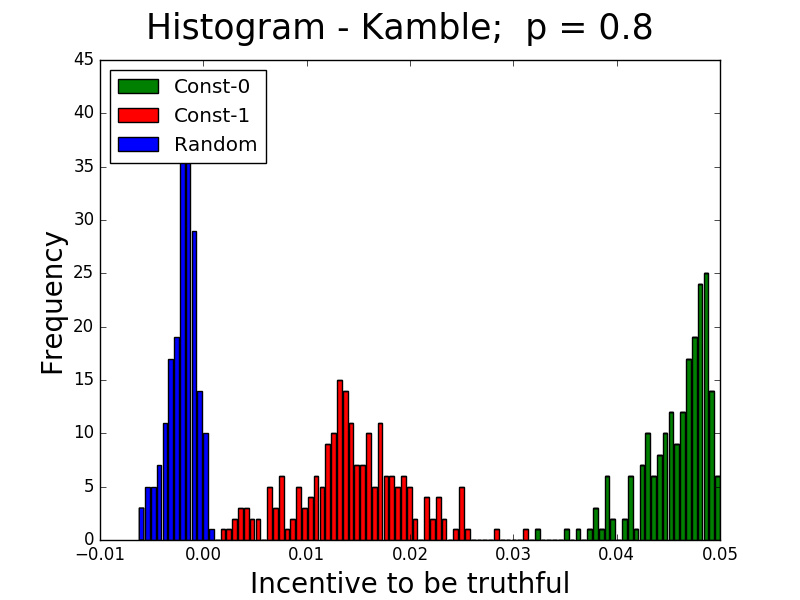
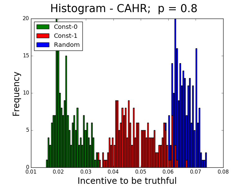
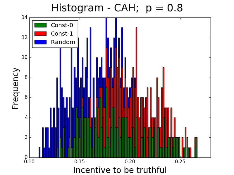
Figure 1: Histograms for the 204 (region, business type) pairs of expected benefit (averaged across questions) from truthful behavior vs. some other strategy, when fraction $0.8$ is truthful and fraction $0.2$ adopt the same, non-truthful strategy.

We observe that the support of the distribution for the CAH and CAHR mechanism is positive, and thus it retains an incentive for truthful behavior. We found this to be a common property for different values of $p$, i.e. CAH and CAHR retains good unilateral incentives for all values of $p$, even when all agents play the same way. By contrast, both the RPTS and Kamble fail under some strategy, i.e. there exists a strategy (random for Kamble and either random or constant-1 for RPTS) such that playing that strategy is more beneficial than playing truthful strategy when some fraction plays this alternate strategy. Although figure 4 shows this for $p=0.8$, this is representative of other values of $p$. The plots for several other values of $p$ are included in Appendix 6.4.

When the prior probability satisfies the self-predicting condition, the RPTS mechanism has truth-telling as a strict equilibrium and the truthful equilibrium provides at least as high payoff than any other coordinated equilibrium where all agents report the same. Since, incentive properties are not proven under RPTS except when the self-predicting condition is satisfied, we evaluated the RPTS mechanism by restricting only to questions that satisfy the self-predicting condition. However, the corresponding plot is similar to the plot shown in figure 4. To conclude, compared to single task mechanisms like RPTS and Kamble, CAH mechanisms provide good guarantees against unilateral deviation.

4.2 Benefit from Coordinated Misreports

Irrespective of whether or not a coordinated deviation is robust against agents choosing to make truthful reports instead, we also consider the expected payoff available to a group of agents who manage to coordinate on some non-truthful play. Figure 2 plots the average and standard error for the expected payments associated with the 204 (region, business type) pairs. For each strategy and for a particular value of $p$, we plot the expected payment and the standard error across the 204 pairs, when $p$ fraction of population is truthful and the remaining $1-p$ fraction of the population adopts the same strategy. The constant line shows the average expected payment across all the pairs when everyone is truthful.

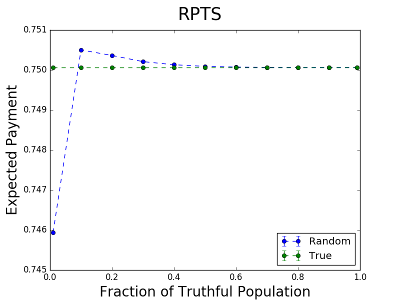
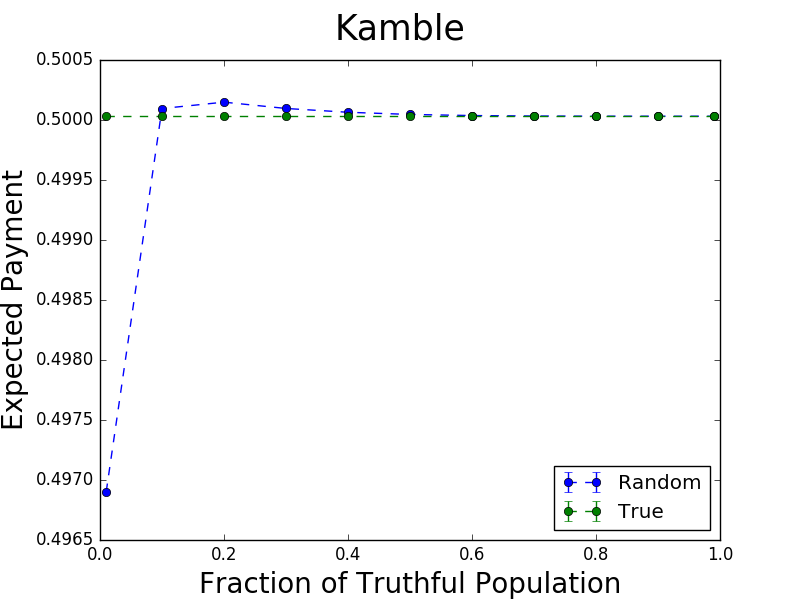
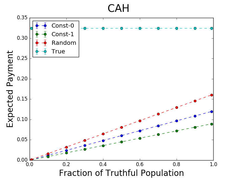
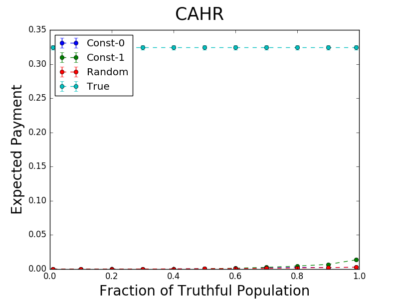
Figure 2: Expected score for following each of four strategies, when $p$ fraction of the population is truthful and $1-p$ fraction adopt the same strategy. Averaged over questions associated with a typical (region, business type) pair.

CAH mechanism has the expected payments from all truthful strategy higher than the other three possible strategies (const-0, const-1 and random) for all possible values of $p$. This means that CAH mechanism is robust against coordinated misreport by any fraction of the population. For RPTS and Kamble, we only plot the expected payments due to the all truthful strategy and the random strategy for various values for $p$. We omit the plots for the expected payments for const-0 and const-1 strategies since the payments under these strategies are significantly lower than the all truthful strategy under both RPTS and Kamble mechanism and do not provide profitable coordinated misreports. We now see that for intermediate values of $p$, the random strategy provide a profitable coordinated misreporting profile under both the RPTS and Kamble mechanism. Therefore, unlike CAH, single task mechanisms like RPTS, Kamble are not always robust to coordinated deviations.

4.3 Subjective vs Factual Tasks

Figure 3 shows the cumulative distribution on expected scores at truthful reporting in each mechanism, where each data point corresponds to a different (region, business type, question) triple. Two lines are shown for each mechanism: one corresponding to questions that are categorized as ‘factual’ and one corresponding to questions that are categorized as ‘subjective.’

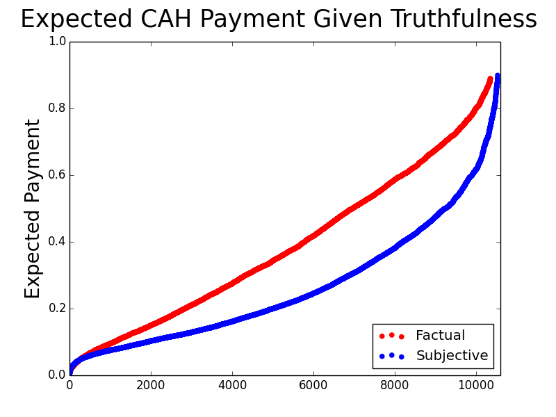
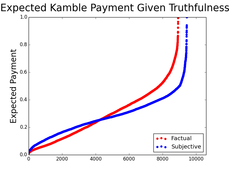
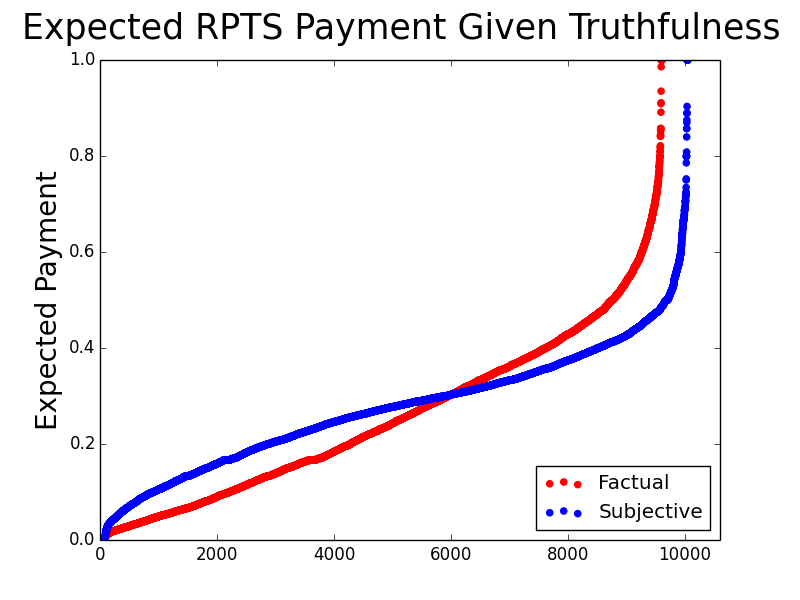
Figure 3: Cumulative distribution on expected payments at truthful reporting in each mechanism, with results separated into questions that are categorized as ‘factual’ and those that are categorized as ‘subjective.’

The subjective questions tend to provide lower expected payment than the factual questions under the CAH mechanism. This is consistent with the intuition that people perceive subjective questions differently than factual questions. For the Kamble and RPTS mechanisms, the variability in expected payment is larger across factual questions than subjective questions, with the expected payment for subjective questions tending to fall in a narrow band.

5 Conclusions

We study the peer prediction problem when users complete heterogeneous tasks. We introduced the CAH mechanism, which is informed-truthful under mild conditions and can also be used together with estimating statistics from reports for the purpose of computing scores. The simulation results suggest that CAH provides better incentive for being truthful and is more resistant to coordinated misreports than the RPTS and Kamble mechanisms. We also noted that CAHR, the empirical version of CAH has similar incentive guarantees, in contrast to the empirical versions of the single-task peer prediction mechanisms. We believe that the theoretical guarantees of the multi-task mechanisms and their attractive incentive properties suggest that such mechanisms are ready to be applied and evaluated in practice, from peer grading to rating. The most important directions for future work are to design mechanisms that can handle agent heterogeneity (agents that vary by taste, judgment, noise, etc.) as well as task heterogeneity. We are also interested in developing specific versions of the CAH mechanism for particular models of heterogeneity, such as the generalized Dawid-Skene scheme (?).

6 Appendix

6.1 Proof of Lemma 1

$$\sum_{i}\sum_{j}\Delta_{b}(i,j)=\sum_{i}\sum_{j}\left\{P_{b}(i,j)\right.$$

$$-\left.\frac{1}{(m-1)(m-2)}\sum_{l^{\prime}\in[m]\setminus\{b\}}\sum_{l^{\prime\prime}\in[m]\setminus\{b,l^{\prime}\}}P_{l^{\prime}}(i)P_{l^{\prime\prime}}(j)\right\}$$

$$=\sum_{i}\left\{P_{b}(i)-\frac{1}{(m-1)(m-2)}\sum_{l^{\prime}\in[m]\setminus\{b\}}\sum_{l^{\prime\prime}\in[m]\setminus\{b,l^{\prime}\}}P_{l^{\prime}}(i)\right\}$$

$$=1-1=0$$

6.2 Proof of Theorem 3

Suppose both the agents adopt the truthful strategy, which corresponds to the identity matrix $\mathbb{I}$. Then the expected payment is given as

$$E(\mathbb{I},\mathbb{I})=\sum_{b=1}^{m}\sum_{i,j:\ \Delta_{b}(i,j)>0}\Delta_{b}(i,j)$$ (5)

On the other hand for any two arbitrary deterministic strategies $F$ and $G$,

$$E(F,G)=\sum_{b=1}^{m}\sum_{i,j}\Delta_{b}(i,j)S_{b}(F_{i},G_{j})\leq\sum_{b=1}^{m}\sum_{i,j:\ \Delta_{b}(i,j)>0}\Delta_{b}(i,j)=E(\mathbb{I},\mathbb{I})$$ (6)

To show strong truthfulness, consider an asymmetric joint strategy $F\neq G$. Then there exists $i$ such that $F_{i}\neq G_{i}$. This reduces the expected payment by at least

$$\sum_{b=1}^{m}\Delta_{b}(i,i)S_{b}(F_{i},G_{i})$$ (7)

Since $F_{i}\neq G_{i}$, we have $\sum_{b=1}^{m}\Delta_{b}(F_{i},G_{i})<0$ and there exists $l^{\prime}$ such that $\Delta_{l^{\prime}}(F_{i},G_{i})<0$ (or $S_{l^{\prime}}(F_{i},G_{i})=0$). Therefore, the expected payment reduces by at least $\Delta_{l^{\prime}}(i,i)>0$.

Now consider symmetric, non-permutation strategy $F=G$. Then there exist $i\neq j$ such that $F_{i}=G_{j}=k$ and the expected payment includes

$$\sum_{b=1}^{m}\Delta_{b}(i,j)S_{b}(k,k)=\sum_{b=1}^{m}\Delta_{b}(i,j)<0$$ (8)

The first equality uses the fact $S_{b}(k,k)=1$ since $\Delta_{b}(k,k)>0$ for each $b$.

6.3 Proof of Theorem 4

We will write $E\left[T,F,G\right]$ to denote the average expected score under strategies $F$ and $G$ when using the score matrix $T=\{T_{b}\}_{b=1}^{m}$. Suppose $S=\{S_{b}\}_{b=1}^{m}$ is the true scoring matrix and $\hat{S}=\{\hat{S}_{b}\}_{b=1}^{m}$ is the scoring matrix estimated from the data. Then

$$E\left[\hat{S},F,G\right]=\frac{1}{m}\sum_{b=1}^{m}\sum_{i,j}\Delta_{b}(i,j)\hat{S}_{b}(F_{i},G_{j})\leq\frac{1}{m}\sum_{b=1}^{m}\sum_{i,j:\Delta_{b}(i,j)>0}\Delta_{b}(i,j)=E\left[S,\mathbb{I},\mathbb{I}\right]$$ (9)

Therefore, in order to show $E\left[\hat{S},\mathbb{I},\mathbb{I}\right]\geq E\left[\hat{S},F,G\right]-\varepsilon$ it is enough to show that $E\left[\hat{S},\mathbb{I},\mathbb{I}\right]\geq E\left[{S},\mathbb{I},\mathbb{I}\right]-\varepsilon$. Now

$$\left|\frac{1}{m}E\left[\hat{S},\mathbb{I},\mathbb{I}\right]-\frac{1}{m}E\left[S,\mathbb{I},\mathbb{I}\right]\right|$$

$$=\left|\frac{1}{m}\sum_{b=1}^{m}\sum_{i,j}\Delta_{b}(i,j)\left(\hat{S}_{b}(i,j)-S_{b}(i,j)\right)\right|=\left|\frac{1}{m}\sum_{b=1}^{m}\sum_{i,j}\Delta_{b}(i,j)\left(\text{sign}\left(\hat{\Delta}_{b}(i,j)\right)-\text{sign}\left(\Delta_{b}(i,j)\right)\right)\right|$$

$$\leq\frac{1}{m}\sum_{b=1}^{m}\sum_{i,j}\left|\Delta_{b}(i,j)\left(\text{sign}\left(\hat{\Delta}_{b}(i,j)\right)-\text{sign}\left(\Delta_{b}(i,j)\right)\right)\right|\leq\frac{1}{m}\sum_{b=1}^{m}\sum_{i,j}\left|\hat{\Delta}_{b}(i,j)-\Delta_{b}(i,j)\right|$$

$$=\frac{1}{m}\sum_{b=1}^{m}\sum_{i,j}\left|P_{b}(i,j)-T_{b}(i,j)-\frac{1}{(m-1)(m-2)}\sum_{\stackrel{{\scriptstyle t^{\prime},t^{\prime\prime}\in[m]\setminus\{b\}}}{{\&\ t^{\prime}\neq t^{\prime\prime}}}}\left(P_{t^{\prime}}(i)P_{t^{\prime\prime}}(j)-T_{t^{\prime}}(i)T_{t^{\prime\prime}}(j)\right)\right|$$

$$\leq\frac{1}{m}\sum_{b=1}^{m}\sum_{i,j}\left|P_{b}(i,j)-T_{b}(i,j)\right|+\frac{1}{(m-1)(m-2)}\sum_{\stackrel{{\scriptstyle t^{\prime},t^{\prime\prime}\in[m]\setminus\{b\}}}{{\&\ t^{\prime}\neq t^{\prime\prime}}}}\left|P_{t^{\prime}}(i)P_{t^{\prime\prime}}(j)-T_{t^{\prime}}(i)T_{t^{\prime\prime}}(j)\right|$$

$$=\frac{1}{m}\sum_{b=1}^{m}\sum_{i,j}\left|P_{b}(i,j)-T_{b}(i,j)\right|+\frac{1}{m(m-1)(m-2)}\sum_{b=1}^{m}\sum_{i,j}\sum_{\stackrel{{\scriptstyle t^{\prime},t^{\prime\prime}\in[m]\setminus\{b\}}}{{\&\ t^{\prime}\neq t^{\prime\prime}}}}\left|P_{t^{\prime}}(i)\left(P_{t^{\prime\prime}}(j)-T_{t^{\prime\prime}}(j)\right)\right.$$

$$+\left.T_{t^{\prime\prime}}(j)\left(P_{t^{\prime}}(i)-T_{t^{\prime}}(i)\right)\right.$$

$$\leq\frac{1}{m}\sum_{b=1}^{m}\sum_{i,j}\left|P_{b}(i,j)-T_{b}(i,j)\right|$$ (10)

$$+\frac{1}{m(m-1)(m-2)}\sum_{b=1}^{m}\sum_{\stackrel{{\scriptstyle t^{\prime},t^{\prime\prime}\in[m]\setminus\{b\}}}{{\&\ t^{\prime}\neq t^{\prime\prime}}}}\left\{\sum_{j}\left|P_{t^{\prime\prime}}(j)-T_{t^{\prime\prime}}(j)\right|\sum_{i}P_{t^{\prime}}(i)\right.+\left.\sum_{i}\left|P_{t^{\prime}}(i)-T_{t^{\prime}}(i)\right|\sum_{j}T_{t^{\prime\prime}}(j)\right\}$$

$$=\frac{1}{m}\sum_{b=1}^{m}\sum_{i,j}\left|P_{b}(i,j)-T_{b}(i,j)\right|$$ (11)

$$+\frac{1}{m(m-1)(m-2)}\sum_{b=1}^{m}\sum_{\stackrel{{\scriptstyle t^{\prime},t^{\prime\prime}\in[m]\setminus\{b\}}}{{\&\ t^{\prime}\neq t^{\prime\prime}}}}\left\{\sum_{j}\left|P_{t^{\prime\prime}}(j)-T_{t^{\prime\prime}}(j)\right|+\sum_{i}\left|P_{t^{\prime}}(i)-T_{t^{\prime}}(i)\right|\right\}$$ (12)

Now if we have $O\left(\frac{n^{2}}{\varepsilon^{2}}\log\left(\frac{m}{\delta}\right)\right)$ samples from each joint distribution $P_{b}$ (where $n$ is the number of signals) and $O\left(\frac{n}{\varepsilon^{2}}\log\left(\frac{m}{\delta}\right)\right)$ from each marginal distribution $P_{b}$, we can ensure that with probability at least $1-\delta$, for all $b=1,2,\ldots,m$ the following results hold (see (?) for a proof)

$$\sum_{i,j}\left|P_{b}(i,j)-T_{b}(i,j)\right|\leq\frac{\varepsilon}{3}\ \text{and}\ \sum_{i}\left|P_{b}(i)-T_{b}(i)\right|\leq\frac{\varepsilon}{3}.$$ (13)

Note: If we just had $O(n/\varepsilon^{2}\log(1/\delta))$ samples for each task, then we can guarantee (13) for each task separately with probability at least $1-\delta$. By the union bound, this would give a success probability of $1-m\delta$ over all tasks. So in order to have a $1-\delta$ confidence bound, we need a $\log(m/\delta)$ factor in the sample complexity. Substituting the bounds from eq. 13 in eq. 12 and simplifying gives us $\left|E\left[\hat{S},\mathbb{I},\mathbb{I}\right]-E\left[S,\mathbb{I},\mathbb{I}\right]\right|\leq\varepsilon$. Since there are $q$ agents providing reviews for each task, we get $q^{2}$ samples from each joint distribution and $q$ samples from each marginal distribution. So as long as $q=\Omega\left(\frac{n}{\varepsilon^{2}}\log\left(\frac{m}{\delta}\right)\right)$ we have enough number of samples and we are done.

6.4 Additional Plots

References

- [Agarwal et al. 2017] Arpit Agarwal, Debmalya Mandal, David C. Parkes, and Nisarg Shah. Peer Prediction with Heterogeneous Users. In Proceedings of the 2017 ACM Conference on Economics and Computation, pages 81–98, 2017.
- [Dasgupta and Ghosh 2013] Anirban Dasgupta and Arpita Ghosh. Crowdsourced Judgement Elicitation with Endogenous Proficiency. In Proceedings of the 22nd international conference on World Wide Web, pages 319–330. ACM, 2013.
- [Dawid and Skene 1979] Alexander P. Dawid and Allan M. Skene. Maximum Likelihood Estimation of Observer Error-Rates Using the EM Algorithm. Applied statistics, pages 20–28, 1979.
- [Devroye and Lugosi 2012] Luc Devroye and Gábor Lugosi. Combinatorial Methods in Density Estimation. Springer Science & Business Media, 2012.
- [Jurca and Faltings 2008] Radu Jurca and Boi Faltings. Truthful Opinions from the Crowds. ACM SIGecom Exchanges, 7(2):3, 2008.
- [Jurca and Faltings 2009] Radu Jurca and Boi Faltings. Mechanisms for Making Crowds Truthful. Journal of Artificial Intelligence Research, 34(1):209, 2009.
- [Kamble et al. 2015] Vijay Kamble, David Marn, Nihar Shah, Abhay Parekh, and Kannan Ramachandran. Truth Serums for Massively Crowdsourced Evaluation Tasks. The 5th Workshop on Social Computing and User-Generated Content, 2015.
- [Kong et al. 2016] Yuqing Kong, Katrina Ligett, and Grant Schoenebeck. Putting Peer Prediction Under the Micro (economic) scope and Making Truth-telling Focal. In International Conference on Web and Internet Economics, pages 251–264. Springer, 2016.
- [Miller et al. 2005] Nolan Miller, Paul Resnick, and Richard Zeckhauser. Eliciting Informative Feedback: The Peer-Prediction method. Management Science, 51:1359–1373, 2005.
- [Radanovic et al. 2016] Goran Radanovic, Boi Faltings, and Radu Jurca. Incentives for Effort in Crowdsourcing Using the Peer Truth Serum. ACM Transactions on Intelligent Systems and Technology (TIST), 7(4):48, 2016.
- [Shnayder et al. 2016a] Victor Shnayder, Arpit Agarwal, Rafael Frongillo, and David C Parkes. Informed Truthfulness in Multi-Task Peer Prediction. In Proceedings of the 2016 ACM Conference on Economics and Computation, pages 179–196. ACM, 2016.
- [Shnayder et al. 2016b] Victor Shnayder, Rafael Frongillo, and David C. Parkes. Measuring performance of peer prediction mechanisms using replicator dynamics. In Proc. 25th International Joint Conference on Artificial Intelligence (IJCAI), pages 2611–2617, 2016.
- [Witkowski and Parkes 2012] Jens Witkowski and David C Parkes. A Robust Bayesian Truth Serum for Small Populations. In Proceedings of the Twenty-Sixth AAAI Conference on Artificial Intelligence (AAAI), pages 1492–1498, 2012.