On the Angular Momentum of Rockets, Balloons, and Other Variable Mass Systems

Abstract

Variable mass systems are a classic example of open systems in classical mechanics. The reaction forces due to mass variation propel ships, balloons, and rockets. Unlike free constant mass systems, the angular momentum of these systems is not of constant magnitude due to the change in mass. In this paper, we show that the angular momentum vector for such a system has a fixed direction in space and, thus, is partially conserved for both rigid and flexible, torque-free, variable mass systems. A potential use of this result is that it provides a suitable stationary reference frame against which the orientation of variable mass system could be measured.

Mass-varying systems have a longstanding history in classical mechanics. According to Šíma and Podolský sima , Buquoy first formulated the equations of motion for a generic variable mass system and also offered some context to its application by examining the vertical motion of an extensible flexible fiber. However, Mikhailov mikhailov considers Bernoulli’s idea of jet-propelled ships bernoulli as the first foray into reaction devices and, thus, moving variable mass systems. Moore moore , around the same time as Buquoy, focused on a different subset of variable mass systems by deriving the classic rocket equation. Since then, most of the academic and engineering discourses on variable mass system dynamics have focused primarily on their application to rockets.

The pioneering works of stalwarts such as Tsiolkovsky tsiolkovsky and Goddard goddard was on understanding the translational dynamics of rockets to escape earth’s gravitational field. However, a flurry of work concentrating on the rotational dynamics of rockets and variable mass systems is seen in the mid-twentieth century. Rosser et al rosser examined the motion of both spinning and non-spinning rockets and are considered to be the first to present the idea of jet damping, apud van der Ha and Janssens vanderha . Forms of the rotational equations that more closely resemble Euler’s rigid body equations are seen in a paper by Ellis and McArthur ellis , and Thomson’s thomsontext classic textbook, with the latter addressing the general variable mass system with discrete mass loss. A more sophisticated model utilizing a control volume approach to account for continuous mass variation was later presented by Thorpe thorpe . This control volume approach has since gained widespread acceptance meirovitch ; cornelisse ; eke ; quadrelli . We consider it interesting to note that, despite interest in variable mass systems beginning in the same era as Euler’s study of rigid body motion, analytical studies into their rotational motion have only been performed over the last 70 years.

Our letter also concerns the rotational dynamics of variable mass systems, wherein we prove the conservation of the direction of angular momentum about the instantaneous mass center. The utility of this result can be understood from the perspective of some developments on constant mass systems’ dynamics. In the case of free constant mass systems, proving the fixedness of the angular momentum vector is a trivial outcome, due to its conservation, but has proved extremely valuable in theory poinsot as well as in practice bracewell ; landon . Poinsot poinsot developed an approach to visualize the motion of asymmetric rotating rigid bodies without explicitly solving the governing nonlinear equations of motion. His work is considered one of the cornerstones in the field of geometric mechanics. Relatively recently, Poinsot’s work was extended to explain the dissipative effects of flexibility on spinning structures, independently by Bracewell and Garriott bracewell , and Landon and Stewart landon . These investigators showed that flexible bodies (without mass variation) rotate stably about the axis of maximum moment of inertia but are unstable about the axes of intermediate and minor moment of inertia, a phenomenon verified by the unstable flight of the Explorer-1 satellite. The fixed nature of the angular momentum vector also permits solutions to orientation angles (e.g. Euler angles) of rotating axisymmetric rigid bodies likins and such analytical results are useful in controlling the motion of bodies. The development of similar literature on variable mass systems can be extremely useful at a time when spaceflight is more commonplace but a better understanding of these systems’ angular momenta is necessary to enable such work.

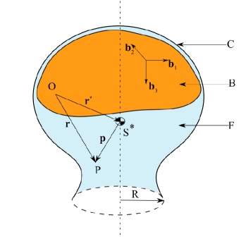
Figure 1: General Variable Mass System

Figure 1 is that of a system with mass variation comprising a consumable rigid base $B$ and a fluid phase $F$. A massless shell $C$ of volume $V_{0}$ and surface area $S_{0}$ is attached to $B$. It is assumed that mass can enter or exit $C$ through the region represented as a dashed ellipse. The shell and everything within it is considered to be of interest, while any matter outside of it is not. At any instant, there is a definite set of matter within the region $C$ which obeys the laws of mechanics. At another instant, $C$ may contain a different set of matter but it too must obey the laws of mechanics at that instant. Thus, the angular momentum principle can be applied to $C$ and its contents to derive the vector equation of attitude motion that are valid at each instant of time.

At any general instant of time there is a definite set of matter within $C$. The angular momentum of this constant mass system about its mass center $S^{*}$, denoted ${\bf H}^{*}$, is given by

$${\bf H}^{*}=\int_{V}\rho{\bf p\times v}\,\mathrm{d}V,$$ (1)

where $V$ is the volume occupied by the contents of the constant mass system at the instant of interest, $\rho$ is the mass density, $\bf p$ is a position vector from $S^{*}$ to an arbitrary particle $P$ within $C$, and $\bf v$ is the inertial velocity of $P$. The motion of $P$ when observed from $B$ allows the above angular momentum expression to be reformulated as

$${\bf H}^{*}=\int_{V}\rho{\bf p}\times[{\bf v}^{o}+{\bf v}_{r}+{\bm{\omega}\times\bf r}]\,\mathrm{d}V,$$ (2)

where $\bf r$ is a position vector from $O$ to $P$, ${\bf v}^{o}$ is the inertial velocity of $O$, ${\bf v}_{r}$ is the velocity of $P$ relative to $B$, and $\bm{\omega}$ is the inertial angular velocity of $B$. Equation (2) is then expanded as

$${\bf H}^{*}=\int_{V}\rho{\bf p}\,\mathrm{d}V\times{\bf v}^{o}+\int_{V}\rho{\bf p}\times{\bf v}_{r}\,d\mathrm{}V+\int_{V}\rho{\bf p}\times({\bm{\omega}\times\bf r})\,\mathrm{d}V,$$ (3)

The first integral on the right-hand side of Equation (3) evaluates to zero by virtue of the definition of a mass center. Further, from Figure 1, it is evident that ${\bf r}={\bf r}^{*}+{\bf p}$ where ${\bf r}^{*}$ is the position vector from $O$ to $S^{*}$ so Equation (3) can be rewritten as

$${\bf H}^{*}=\int_{V}\rho{\bf p} \times{\bf v}_{r}\,\mathrm{d}V+\int_{V}\rho{\bf p}\times({\bm{\omega}\times{\bf r}^{*}})\,\mathrm{d}V+\int_{V}\rho{\bf p}\times({\bm{\omega}\times{\bf p}})\,\mathrm{d}V.$$ (4)

The second volume integral on the right-hand side of Equation (4) evaluates to zero, again, by the principle of mass centers. Equation (4) is now written in a compact form as

$${\bf H}^{*}=\int_{V}\rho{\bf h}\,\mathrm{d}V,$$ (5)

where ${\bf h}$ is

$${\bf h}\triangleq{\bf p\times[{\bf v}_{r}+(\bm{\omega}\times p})].$$ (6)

Equation (5) now gives the instantaneous angular momentum of a constant mass system. The angular momentum principle applied to this constant mass system about its mass center is

$${\bf M}^{*}=\frac{{}^{N}\mathrm{D}{\bf H}^{*}}{\mathrm{D}t},$$ (7)

where ${\bf M}^{*}$ is the sum of all moments due to external forces on the constant mass system, and $\frac{{}^{N}\mathrm{D}}{\mathrm{D}t}$ is the material derivative observed from an inertial frame $N$. In the case of torque-free motion, ${\bf M}^{*}={\bf 0}$ which when used in Equation (7) gives

$${\bf 0}=\frac{{}^{N}\mathrm{D}}{\mathrm{D}t}\int_{V}\rho{\bf h}\,\mathrm{d}V.$$ (8)

Note that, in Equation (8), ${\bf H}^{*}$ has been expressed in its integral form, given by Equation (5). The above equation tells us that the angular momentum of the constant mass system is invariant. If we choose to switch from the inertial reference frame to a reference frame attached to $B$ then Equation (8) can be rewritten as

$${\bf 0}=\frac{{}^{B}\mathrm{D}}{\mathrm{D}t}\int_{V}\rho{\bf h}\,\mathrm{d}V+\bm{\omega}\times\int_{V}\rho{\bf h}\,\mathrm{d}V.$$ (9)

In the above form, the two terms on the right hand side of Equation (9) focus on the constant mass system. Attention can be transferred to the control volume with fluxing matter via two operations. Firstly, Reynolds’ Transport Theorem is invoked on the first term on the right-hand side of Equation (9). Secondly, noticing that, at the instant for which the above equation is derived, $V=V_{0}$. As a result, Equation (9) becomes

$${\bf 0}=\frac{{}^{B}\mathrm{d}}{dt}\int_{V_{0}}\rho{\bf h}\,\mathrm{d}V+\int_{S_{0}}\rho{\bf h}({\bf v}_{r}\cdot{\hat{\bf n}})\,\mathrm{d}S+\bm{\omega}\times\int_{V}\rho{\bf h}\,\mathrm{d}V.$$ (10)

In the above equation, $\hat{\bf n}$ is an outwardly directed unit normal from a surface of $C$ through which mass enters and/or exits. If ${\bf v}_{r}\cdot{\hat{\bf n}}=u$, where $u$ is a general scalar variable, Equation (10) can be rewritten as

$${\bf 0}=\frac{{}^{B}\mathrm{d}{\bf H}^{*}_{0}}{\mathrm{d}t}+\int_{S_{0}}\rho{\bf h}u\,\mathrm{d}S+\bm{\omega}\times{\bf H}_{0}^{*},$$ (11)

where ${\bf H}^{*}_{0}$ is the angular momentum of the variable mass system and is

$${\bf H}^{*}_{0}=\int_{V_{0}}\rho{\bf h}\,\mathrm{d}V.$$ (12)

Since $V=V_{0}$ at a particular instant, ${\bf H}^{*}$ and ${\bf H}_{0}^{*}$ are identical but their time derivatives are generally not identical since their evolution in time is associated with changing sets of matter. Since our interest is in understanding the behaviour of the variable mass system’s angular momentum from an inertial frame, we revert the time derivative in Equation (11) to $N$

$${\bf 0}=\frac{{}^{N}\mathrm{d}{\bf H}^{*}_{0}}{\mathrm{d}t}+\int_{S_{0}}\rho{\bf h}u\,\mathrm{d}S.$$ (13)

Any vector can be expressed as a combination of a scalar and a unit vector directed along the vector itself. So, $\bf h$ is rewritten as ${\bf h}=h{\hat{\bf n}_{h}}$, where ${\hat{\bf n}_{h}}$ is a unit vector directed along $\bf h$ whose magnitude is $h$. As a result, Equation (12) can be written as

$${\bf H}^{*}_{o}=\bigg{(}\int_{V_{o}}\rho h\,\mathrm{d}V\bigg{)}{\hat{\bf n}_{h}}$$ (14)

and Equation (13) as

$$\frac{{}^{N}\mathrm{d}{\bf H}^{*}_{o}}{\mathrm{d}t}=\bigg{(}-\int_{S_{o}}\rho hu\,\mathrm{d}S\bigg{)}{\hat{\bf n}_{h}}$$ (15)

Equation (14) asserts that ${\bf H}^{*}_{o}$ is not of constant magnitude while Equations (14) and (15) assert that it is always directed along the $\hat{\bf n}_{h}$ vector, which it will now be proved is an inertially fixed vector.

Let $\hat{\bf n}_{f}$ and $\hat{\bf n}_{g}$ be two unit vectors which form a dextral set with $\hat{\bf n}_{h}$, then $\hat{\bf n}_{f}\times\hat{\bf n}_{g}=\hat{\bf n}_{h}$ and so on. This dextral set of unit vectors are attached to an imaginary reference frame $Q$ whose inertial angular velocity is expressed as

$${\bm{\omega}}^{Q}=\Omega_{1}\hat{\bf n}_{f}+\Omega_{2}\hat{\bf n}_{g}+\Omega_{3}\hat{\bf n}_{h}.$$ (16)

The time rate of change of $\hat{\bf n}_{h}$ in the inertial frame is

$$\frac{{}^{N}{\mathrm{d}}\hat{\bf n}_{h}}{\mathrm{d}t}=\frac{{}^{Q}\mathrm{d}\hat{\bf n}_{h}}{\mathrm{d}t}+{\bm{\omega}}^{Q}\times\hat{\bf n}_{h}$$ (17)

where the first term on the right-hand side of Equation (17) evaluates to zero since $\hat{\bf n}_{h}$ is fixed in $Q$. Then, substituting for $\bm{\omega}^{Q}$ from Equation (16) in Equation (17) gives

$$\frac{{}^{N}{\mathrm{d}}\hat{\bf n}_{h}}{\mathrm{d}t}=\Omega_{2}\hat{\bf n}_{f}-\Omega_{1}\hat{\bf n}_{g}.$$ (18)

Further, Equation (15) is rewritten as

$$\frac{{}^{N}\mathrm{d}}{\mathrm{d}t}\int_{V_{o}}\rho h\,\mathrm{d}V\hat{\bf n}_{h}=\bigg{(}-\int_{S_{o}}\rho uh\,\mathrm{d}S\bigg{)}\hat{\bf n}_{h}$$ (19)

or

$$\frac{\mathrm{d}}{\mathrm{d}t}\bigg{(}\int_{V_{o}}\rho h\,{\mathrm{d}}V\bigg{)}\hat{\bf n}_{h}+\bigg{(}\int_{V_{o}}\rho h\,\mathrm{d}V\bigg{)}\frac{{}^{N}{\mathrm{d}}{\hat{\bf n}_{h}}}{\mathrm{d}t}\\ =\bigg{(}-\int_{S_{o}}\rho uh\,\mathrm{d}S\bigg{)}\hat{\bf n}_{h}.$$ (20)

The result from Equation (18) is substituted in Equation (20) to give

$$\frac{\mathrm{d}}{\mathrm{d}t}\bigg{(}\int_{V_{o}} \rho h\,{\mathrm{d}}V\bigg{)}\hat{\bf n}_{h}+\bigg{(}\int_{V_{o}}\rho h\,{\mathrm{d}}V\bigg{)}(\Omega_{2}\hat{\bf n}_{f}-\Omega_{1}\hat{\bf n}_{g})$$ (21)

$$=\bigg{(}-\int_{S_{o}}\rho uh\,{\mathrm{d}}S\bigg{)}\hat{\bf n}_{h}.$$

The above equation, when rewritten in component form, leads to $\Omega_{1}=\Omega_{2}=0$. Using these values for $\Omega_{1}$ and $\Omega_{2}$ in Equation (18) gives $\frac{{}^{N}d\hat{\bf n}_{h}}{dt}={\bf 0}$, which explains that $\hat{\bf n}_{h}$ is an inertially fixed unit vector thus, also making $Q$ an inertial frame. By extension, it can be inferred that the angular momentum of a variable mass system is also an inertially fixed vector as it is directed along $\hat{\bf n}_{h}$.

Through this write-up it has been shown that the angular momentum of a variable mass system is inertially fixed despite its variable magnitude. As mentioned in the earlier portions of this text, this result can serve as the foundation for analytical and geometric examinations of the rotational motions of variable mass systems in a manner similar to that seen in the literature on rigid bodies. For example, one may attempt to perform a stability analysis of rotating variable mass systems. Further, as the theory developed here is applicable to flexible systems it can be useful in studies on engineering systems such as rockets, and balloons. This result can also find application in navigation and control of underwater vehicles which are modeled using a control volume approach.

References

- (1) G.K. Mikhailov, in Landmark Writings in Western Mathematics 1640-1940 (Elsevier Science, Amsterdam, 2005), pp. 131-142.
- (2) D. Bernoulli, Hydrodynamica sive de viribus et motibus fluidorum commentarii. Johann Reinhold Dulsecker, 1738.
- (3) Šíma, Vladimír and Podolskỳ, Jiří, Buquoy’s Problem. European Journal of Physics, 26(6), 1037, (2005).
- (4) W. Moore, A treatise on the motion of rockets. London: G. and S. Robinson (1813)
- (5) K. E. Tsiolkovsky, Exploration of the Universe with Reaction Machines, in John M. Logsdon, ed., Exploring the Unknown: Selected Documents in the History of the U.S. Space Program, vol. 1 (Washington, D.C.: National Aeronautics and Space Administration, 1995), 59–83.
- (6) Goddard, R. H. (1920).A Method of Reaching Extreme Altitudes. Nature, 105, 809-811.
- (7) J.B. Rosser J, R.R. Newton, and G.L. Gross, Mathematical Theory Of Rocket Flight (McGraw Hill Book Company Inc., 1947).
- (8) van der Ha, J.C., Janssens, F.L.: Jet-Damping and Misalignment Effects During Solid-Rocket-Motor Burn. Journal of Guidance, Control, and Dynamics. 28, 412-420 (2005).
- (9) Ellis, J. W., and McArthur, C. W. (1959). Applicability of Euler’s dynamical equations to rocket motion. ARS Journal, 29(11), 863-864.
- (10) Thomson, W.T.: Introduction to Space Dynamics (Chapter 7). Dover, New York (1986).
- (11) Thorpe, J. F. (1962). On the momentum theorem for a continuous system of variable mass. Am. J. Phys, 30, 637-640.
- (12) L. Meirovitch, General motion of a variable-mass flexible rocket with internal flow. Journal of Spacecraft and Rockets 7, 186 (1970).
- (13) J.W. Cornelisse, H.F.R. Schöyer, and K.F. Wakker, Rocket Propulsion and Spaceflight Dynamics, (Pitman, London; San Francisco, 1979).
- (14) F.O. Eke and S.M. Wang, Equations of Motion of Two-phase Variable Mass Systems with Solid Base. Journal of Applied Mechanics 61, 855 (1994).
- (15) Marco B. Quadrelli, Jonathan M. Cameron, and Bob Balaram. Modeling and Simulation of Flight Dynamics of Variable Mass Systems, AIAA/AAS Astrodynamics Specialist Conference, 4-7 August 2014, San Diego, (AIAA 2014-4454)
- (16) L. Poinsot, Théorie Nouvelle de La Rotation Des Corps, (Bachelier, 1851).
- (17) Bracewell, R. N. and Garriott, O. K., Rotation of artificial earth satellites, Nature 182 , 760-762 (September, 02 1958).
- (18) Landon, Vernon D., and Brian Stewart. Nutational stability of an axisymmetric body containing a rotor. Journal of Spacecraft and Rockets 1, no. 6 (1964): 682-684.
- (19) H. Goldstein, C. Poole, and J. Safko, Classical Mechanics (3rd Ed.) (Addison-Wesley, 2001).
- (20) P.W. Likins, Elements of Engineering Mechanics, (McGraw-Hill, 1973).