FRIDA: FRI-BASED DOA ESTIMATION FOR ARBITRARY ARRAY LAYOUTS

Abstract

In this paper we present FRIDA—an algorithm for estimating directions of arrival of multiple wideband sound sources. FRIDA combines multi-band information coherently and achieves state-of-the-art resolution at extremely low signal-to-noise ratios. It works for arbitrary array layouts, but unlike the various steered response power and subspace methods, it does not require a grid search. FRIDA leverages recent advances in sampling signals with a finite rate of innovation. It is based on the insight that for any array layout, the entries of the spatial covariance matrix can be linearly transformed into a uniformly sampled sum of sinusoids.

Index Terms— Direction of arrival, finite rate of innovation, subspace method, search-free, wideband sources

1 Introduction

A wishlist for a direction of arrival (DOA) estimator may look something like this: it should be high-resolution, work at low signal-to-noise ratios (SNRs), resolve many possibly closely spaced sources, work with few arbitrarily laid out microphones, and do so efficiently, without grid searches.

It is uncommon to have all of these items checked at once. For example, the steered response power (SRP) methods [1] can be made robust, do not require a specific array geometry, and are immune to coherence in signals. Because they are based on beamforming though, they cannot resolve close sources [2].

Close sources can be resolved by the high-resolution DOA finders. Their main representatives are subspace methods such as MUSIC [3], Prony-type methods such as root-MUSIC [4], and methods that attempt to compute the maximum likelihood (ML) estimator such as IQML [5].

Subspace methods exploit the fact that for uncorrelated signal and noise, the eigenspace of the spatial covariance matrix corresponding to largest eigenvalues is spanned by the source steering vectors [3]. These methods are fundamentally narrowband since the signal subspaces vary with frequency; they can be made wideband either by incoherently combining narrowband estimates or, better, by combining them coherently through transforming the array manifold at each frequency to a manifold at a reference frequency (CSSM [6], WAVES [7]). These methods require a search over space unless the array is a uniform linear array (ULA) [8]. Coherent methods also require special “focusing matrices”, essentially initial guesses of the source locations. WAVES can do without focusing but at the cost of performance. In between coherent and incoherent methods is the TOPS algorithm [9], which performs well at mid-SNRs, but still requires a search and performs worse than coherent methods at low SNRs.

We propose a new finite rate of innovation (FRI) sampling-based algorithm for DOA finding—FRIDA. Among the mentioned algorithms, FRIDA is most reminiscent of IQML [5], especially for narrowband signals and ULAs. Unlike IQML, FRIDA works for arbitrary sensor geometries and for wideband signals. Moreover, it uses multi-band information coherently. Still, it requires no grid search and no sensitive preprocessing akin to focusing matrices, and it achieves very high resolution at very low SNRs, outperforming previous state-of-the-art.

FRIDA can work with fewer microphones than sources as it uses cross-correlations instead of raw microphone streams. The tradeoff is that it is not able to handle completely correlated signals. A straightforward modification of the algorithm which operates on raw signals rather than cross-correlations does not have this issue, but it requires more microphones.

The main ingredient of FRIDA is an FRI sampling algorithm [10]. FRI sampling has recently been extended to non-uniform grids along with a robust reconstruction algorithm [11]. The algorithm is an iterative algorithm similar to IQML, but with an added spectral resampling layer and a modified stopping criterion (Section 2.2.3). The key insight is that the elements of the spatial correlation matrix can be linearly transformed into uniformly sampled sums of sinusoids, regardless of the array geometry.

2 Notation and Problem Formulation

Throughout the paper, matrices and vectors are denoted by bold upper and lower case letters. The Euclidean norm of a vector ${\rm\bf x}$ is denoted by $\|{\rm\bf x}\|_{2}=({\rm\bf x}^{\mbox{\tiny\sc H}}{\rm\bf x})^{\nicefrac{{1}}{{2}}}$. We denote by $\mathbb{S}$ the unit circle. Unit propagation vectors will be denoted by $\bm{p}$.

2.1 Source Signal and Measurements

2.1.1 Sources with Arbitrary Spatial Support

We assume a setup with $Q$ microphones located at $\{\bm{r}_{q}\in\mathbb{R}^{2}\}_{q=1}^{Q}$, and $K$ monochromatic and uncorrelated point sources in the far-field indexed by the letter $k$. Each propagates in the direction of the unit vector $\bm{p}_{k}\in\mathbb{S}$. Within a narrow band centered at frequency $\omega$, the baseband representation of the signal coming from direction $\bm{p}\in\mathbb{S}$ reads $x(\bm{p},\omega,t)=\tilde{x}(\bm{p},\omega){\rm e}^{j\omega t},$where $\tilde{x}(\bm{p},\omega)$ is the emitted sound signal by a source located at $\bm{p}$ and frequency $\omega$. The intensity of the sound field is then

$$I(\bm{p},\omega)\stackrel{{\scriptstyle{\rm def}}}{{=}}\mathbb{E}\left[|x(\bm{p},\omega,t)|^{2}\right]=\mathbb{E}\left[|\tilde{x}(\bm{p},\omega)|^{2}\right].$$ (1)

We assume frame-based processing, and the expectation is over the randomness of $\tilde{x}$ from frame to frame. As $\tilde{x}$ carries the phase, the assumption $\mathbb{E}\left[\tilde{x}\right]=0$ holds. Note that at this point we did not yet make the point source assumption.

The received signal at the $q$-th microphone located at $\bm{r}_{q}$ is the integration of all plane waves along the unit circle:

$$y_{q}(\omega,t)=\int_{\mathbb{S}}x(\bm{p},\omega,t){\rm e}^{-j\omega\left\langle\bm{p},\frac{\bm{r}_{q}}{c}\right\rangle}\,{\mathrm{d}}\bm{p}\quad\text{for }q=1,\cdots,Q,$$ (2)

where $c$ is the speed of sound. In this paper, we will take as measurements the cross-correlations between the received signals for a microphone pair $(q,q^{\prime})$:

$$V_{q,q^{\prime}}(\omega)\stackrel{{\scriptstyle{\rm def}}}{{=}}\mathbb{E}\left[y_{q}(\omega,t)y_{q^{\prime}}^{*}(\omega,t)\right]$$ (3)

for $q,q^{\prime}\in[1,Q]$ and $q\neq q^{\prime}$. In practice, $V_{q,q^{\prime}}$ is estimated by averaging over frames; for simplicity we use the same symbol for the empirical version.

If we assume that these sources are spatially uncorrelated, then the cross-correlation reduces to:

$$V_{q,q^{\prime}}(\omega)\!= \!\int_{\mathbb{S}}\!\int_{\mathbb{S}}\!\mathbb{E}\left[x(\bm{p},t)x^{*}(\bm{p}^{\prime},t)\right]\!{\rm e}^{-j\omega\left\langle\!\bm{p},\frac{\bm{r}_{q}}{c}\!\right\rangle}\!{\rm e}^{j\omega\left\langle\!\bm{p}^{\prime},\frac{\bm{r}_{q^{\prime}}}{c}\!\right\rangle}\!\!\,{\mathrm{d}}\bm{p}\!\,{\mathrm{d}}\bm{p}^{\prime}$$ (4)

$$= \int_{\mathbb{S}}I(\bm{p},\omega){\rm e}^{-j\omega\left\langle\bm{p},\Delta\bm{r}_{q,q^{\prime}}\right\rangle}\,{\mathrm{d}}\bm{p},$$ (5)

where $\Delta\bm{r}_{q,q^{\prime}}\stackrel{{\scriptstyle{\rm def}}}{{=}}\frac{\bm{r}_{q}-\bm{r}_{q^{\prime}}}{c}$ is the normalized baseline.

2.1.2 Point Sources

Assume now that our source distribution is a sum of spatially localized sources. We can write

$$\tilde{x}(\bm{p},\omega)=\sum_{k=1}^{K}\alpha_{k}(\omega)\sqrt{\gamma}\phi\big{(}\gamma(\bm{p}-\bm{p}_{k})\big{)}$$ (6)

where $\phi(\bm{p})$ is a localized function with finite energy, $\int\phi^{2}\,{\mathrm{d}}\bm{p}=1$, and $\gamma$ is the spatial scaling factor. To ensure that the $k$-th source has finite power equal to $\sigma_{k}^{2}$, we ask that$\int\mathbb{E}\left[|\alpha_{k}|^{2}\gamma\phi^{2}(\gamma\bm{p})\right]\,{\mathrm{d}}\bm{p}=\sigma_{k}^{2}$ yielding $\mathbb{E}\left[|\alpha_{k}|^{2}\right]=\sigma_{k}^{2}$. If we now denote the intensity corresponding to (6) by $I_{\gamma}(\bm{p},\omega)$, then in the point source limit we get

$$\lim_{\gamma\to 0}I_{\gamma}(\bm{p},\omega)=:I(\bm{p},\omega)=\sum_{k=1}^{K}\sigma_{k}^{2}(\omega)\delta(\bm{p}-\bm{p}_{k}),$$ (7)

where $\sigma_{k}^{2}(\omega)=\mathbb{E}\left[|\tilde{x}(\bm{p}_{k},\omega)|^{2}\right]$, $\bm{p}_{k}=(\cos\varphi_{k},\sin\varphi_{k})^{\mbox{\tiny\sc T}}$, and $\varphi_{k}$ is the azimuth of the $k$-th source.

With the above established, we rewrite the microphone cross-correlations (5) as

$$V_{q,q^{\prime}}(\omega) =\sum_{k=1}^{K}\sigma_{k}^{2}(\omega){\rm e}^{-j\omega\left\langle\bm{p}_{k},\Delta\bm{r}_{q,q^{\prime}}\right\rangle}$$ (8)

for $q\neq q^{\prime}$. Instead of the more conventional approach to FRI sampling where the microphone signals $y_{q}$ would be used as input [12], we use as input the correlations $V_{q,q^{\prime}}$. This effectively increases the number of measurements and allows us to use a small number of microphones.

2.2 Point Source Reconstruction

Following the generalized FRI sampling framework [11], we will first identify the set of unknown sinusoidal samples and its relation with the given measurements (3). Then, the DOA estimation is cast as a constrained optimization (see e.g., (15)).

2.2.1 Relation between Measurements and the Uniform Samples of Sinusoids

Since $\bm{p}$ is supported on the circle, we have the following Fourier series representation for intensity:

$$I(\bm{p},\omega)=\sum_{m\in\mathbb{Z}}\hat{I}_{m}(\omega)Y_{m}(\bm{p}),$$ (9)

where $Y_{m}(\bm{p})$ is the Fourier series basis $Y_{m}(\bm{p})=Y_{m}(\varphi)={\rm e}^{jm\varphi}$, and $\hat{I}_{m}(\omega)$ is the associated expansion coefficient for a sub-band centered at frequency $\omega$:

$$\hat{I}_{m}(\omega)=\!\frac{1}{2\pi}\!\int_{\mathbb{S}}\!I(\bm{p},\omega)Y_{m}^{*}(\bm{p})\,{\mathrm{d}}\bm{p}\!=\!\frac{1}{2\pi}\!\sum_{k=1}^{K}\!\sigma_{k}^{2}(\omega){\rm e}^{-jm\varphi_{k}}\!.$$ (10)

Notice that the Fourier series coefficients $\hat{I}_{m}(\omega)$ for $m\in\mathbb{Z}$ are uniform samples of sinusoids, which are related with the cross-correlation (5) as:

$$V_{q,q^{\prime}}(\omega)=\int_{\mathbb{S}}\sum_{m\in\mathbb{Z}}\hat{I}_{m}(\omega)Y_{m}(\bm{p}){\rm e}^{-j\omega\left\langle\bm{p},\Delta\bm{r}_{q,q^{\prime}}\right\rangle}\,{\mathrm{d}}\bm{p}$$ (11)

$$\stackrel{{\scriptstyle(a)}}{{=}}2\pi\!\sum_{m\in\mathbb{Z}}\!(-j)^{m}J_{m}\left\lparen\|\omega\Delta\bm{r}_{q,q^{\prime}}\|_{2}\right\rparen Y_{m}\left\lparen\!\frac{\Delta\bm{r}_{q,q^{\prime}}}{\|\Delta\bm{r}_{q,q^{\prime}}\|_{2}}\!\right\rparen\hat{I}_{m}$$ (12)

where $(a)$ is from Jacobi-Anger expansion [13] of the complex exponential and $J_{m}(\cdot)$ is Bessel function of the first kind.

Therefore, we establish a linear mapping from the uniformly sampled sinusoids $\hat{I}_{m}$ to the given measurements $V_{q,q^{\prime}}$. Concretely, denote a lexicographically ordered vectorization of the cross-correlations $V_{q,q^{\prime}}(\omega)$, $q\neq q^{\prime}$ by ${\rm\bf a}(\omega)\in\mathbb{C}^{Q(Q-1)}$, and let the vector ${\rm\bf b}(\omega)$ be the Fourier series coefficients $\hat{I}_{m}(\omega)$ for $m\in\cal{M}$, where $\cal{M}$ is a set of considered Fourier coefficients. Define also a $Q(Q-1)\times|{\cal M}|$ matrix ${\rm\bf G}(\omega)$ as

$$g_{(q,q^{\prime}),m}(\omega)\stackrel{{\scriptstyle{\rm def}}}{{=}}(-j)^{m}J_{m}\left\lparen\|\omega\Delta\bm{r}_{q,q^{\prime}}\|_{2}\right\rparen Y_{m}\left\lparen\frac{\Delta\bm{r}_{q,q^{\prime}}}{\|\Delta\bm{r}_{q,q^{\prime}}\|_{2}}\right\rparen,$$ (13)

where rows of ${\rm\bf G}$ are indexed by microphone pairs $(q,q^{\prime})$, and columns of ${\rm\bf G}$ are indexed by Fourier bins $m$. We can then concisely write (12) as ${\rm\bf a}(\omega)={\rm\bf G}(\omega){\rm\bf b}(\omega).$

2.2.2 Annihilation on the Circle

Since $\hat{I}_{m}$ in (10) is a weighted sum of uniformly sampled sinusoids, we know that $\hat{I}_{m}$ should satisfy a set of annihilation equations [10]: $\hat{I}_{m}\mathop{*}h_{m}=0.$ Here $h_{m}$ is the unknown annihilating filters to be recovered. A polynomial, whose coefficients are specified by the filter $h_{m}$, has roots located at ${\rm e}^{-j\varphi_{k}}$ [10]. The source azimuths $\varphi_{k}$ are subsequently reconstructed with polynomial root-finding.

In a multi-band setting, the uniform sinusoidal samples $\hat{I}_{m}(\omega)$ are different for each sub-band. This is because, the signal power $\sigma_{k}^{2}$ varies with the mid-band frequency $\omega$ in general. However, since we have the same source locations $\varphi_{k}$ for each sub-band, we only need to find one filter $h_{m}$ (depending solely on the source locations $\varphi_{k}$) that annihilates $\hat{I}_{m}(\omega)$ for all $\omega$-s:

$$\hat{I}_{m}(\omega)\mathop{*}_{m}h_{m}=0\quad\forall\omega.$$ (14)

2.2.3 Reconstruction Algorithm

Following the discussion in the previous section, we reconstruct the source locations jointly across all sub-bands. More specifically, suppose we consider $J$ sub-bands centered around frequencies $\{\omega_{j}\}_{j=1}^{J}$. Then, we formulate the FRIDA estimate as a solution of the following constrained optimization:

$$\min_{\begin{subarray}{c}{\rm\bf b}_{1},\cdots,{\rm\bf b}_{J}\\ {\rm\bf h}\in\mathcal{H}\end{subarray}} \sum_{i=1}^{J}\big{\|}{\rm\bf a}_{i}-{\rm\bf G}_{i}{\rm\bf b}_{i}\big{\|}_{2}^{2}$$ (15)

subject to $${\rm\bf b}_{i}*{\rm\bf h}={\rm\bf 0}\quad\text{for }i=1,\cdots,J,$$

Here ${\rm\bf a}_{i}$, ${\rm\bf b}_{i}$ and ${\rm\bf G}_{i}$ are the cross-correlation, uniform sinusoidal samples, and the linear mapping between them for the $i$-th sub-band as specified in Section 2.2.1; $\mathcal{H}$ is a feasible set that the annihilating filter coefficients belong to, e.g., $\|{\rm\bf h}\|_{2}^{2}=1$.

Note that (15) is a simple quadratic minimization with respect to ${\rm\bf b}_{i}$-s for a given annihilating filter ${\rm\bf h}$. By substituting the solution of ${\rm\bf b}_{i}$ (in function of ${\rm\bf h}$), we end up with an optimization for ${\rm\bf h}$ alone:

$$\min_{{\rm\bf h}\in\mathcal{H}}\quad{\rm\bf h}^{\mbox{\tiny\sc H}}\bm{\Lambda}({\rm\bf h}){\rm\bf h},$$ (16)

where

$$\bm{\Lambda}({\rm\bf h})\!=\!\sum_{i=1}^{J}{\rm\bf T}^{\mbox{\tiny\sc H}}(\bm{\beta}_{i})\left[{\rm\bf R}({\rm\bf h})\left\lparen{\rm\bf G}_{i}^{\mbox{\tiny\sc H}}{\rm\bf G}_{i}\right\rparen^{-1}{\rm\bf R}^{\mbox{\tiny\sc H}}({\rm\bf h})\right]^{-1}{\rm\bf T}(\bm{\beta}_{i}).$$

Here $\bm{\beta}_{i}=({\rm\bf G}_{i}^{\mbox{\tiny\sc H}}{\rm\bf G}_{i})^{-1}{\rm\bf G}_{i}^{\mbox{\tiny\sc H}}{\rm\bf a}_{i}$; ${\rm\bf T}(\cdot)$ builds a Toeplitz matrix from the input vector; and ${\rm\bf R}(\cdot)$ is the right-dual matrix associated with ${\rm\bf T}(\cdot)$ such that ${\rm\bf T}({\rm\bf b}){\rm\bf h}={\rm\bf R}({\rm\bf h}){\rm\bf b}$, $\forall{\rm\bf b},{\rm\bf h}$. This follows from the commutativity of convolution: ${\rm\bf b}*{\rm\bf h}={\rm\bf h}*{\rm\bf b}$.

In general, it is challenging to solve (16) directly. We use an iterative strategy, building $\Lambda({\rm\bf h})$ with the reconstructed ${\rm\bf h}$ from the previous iteration. However, unlike similar approaches (e.g. [5]), we do not aim at obtaining a convergent solution of (16) but rather a valid solution such that the reconstructed sinusoidal samples ${\rm\bf b}_{i}$-s explain the given measurements up to a certain approximation level ($\varepsilon^{2}$): $\sum_{i=1}^{J}\|{\rm\bf a}_{i}-{\rm\bf G}_{i}{\rm\bf b}_{i}\|_{2}^{2}\leq\varepsilon^{2}$. Readers are referred to [11] for detailed discussions on the algorithmic details, e.g., choice of $\varepsilon$, implementation details, etc.

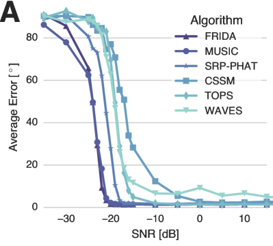
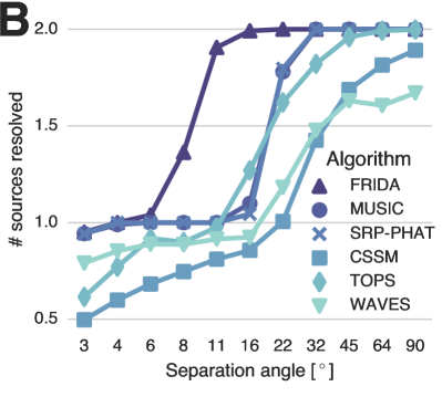
Fig. 1: A Average DOA reconstruction error as a function of SNR. Lower is better. B Average number of sources reconstructed for the case of two sources separated by a fixed angle.

3 Experiments

In this section, we demonstrate the effectiveness of the proposed algorithm through numerical simulations and practical experiments. We compare the performance of FRIDA to that of other wideband algorithms: incoherent MUSIC [3], SRP-PHAT [2], CSSM [6], WAVES [7], and TOPS [9].

The sampling frequency is fixed at $16$ kHz. The narrow-band sub-carriers are extracted by a $256$-point short-time Fourier transform (STFT) with a Hanning window and no overlap. We use a triangular array of $24$ microphones. Each edge is $30$ cm long and carries $8$ microphones. The spacing of microphones ranges from $8$ mm to $25$ cm. This geometry is that of the Pyramic compact array designed at EPFL [14] and used to collect the recordings for the practical experiments, see Fig. 2A.

The number of frequency bands used (out of the $128$ narrow-bands) is a key parameter for performance and was tuned for each algorithm. FRIDA, MUSIC and SRP-PHAT use 20 bands, CSSM and WAVES 10 bands, and TOPS 60 bands. In the synthetic experiments, the source signals are all white noise to simplify the choice of the sub-bands. For speech recordings, the STFT bins with the largest power are chosen. All implementation details are in the supplementary material.

The reconstruction errors are quantified according to the distance on the unit circle defined as

$$d_{\mathbb{S}}(\varphi,\hat{\varphi})=\min_{s\in\{\pm 1\}}s\,(\varphi-\hat{\varphi})\bmod 2\pi.$$ (17)

For multiple DOA, the originals and their reconstructions are matched to minimize the sum of errors.(17)

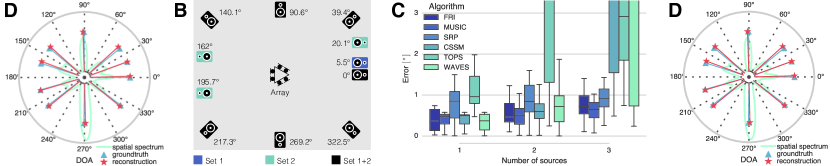
Fig. 2: A Pyramic array, a compact microphone array with $48$ MEMS microphones distributed on the edges of a tetrahedron. For the experiments, only the top triangle is used. B Locations of the loudspeakers and microphone array in experiments. C Reconstruction error for the different algorithms applied to the recorded speech signals. D Reconstruction of $10$ sources from only $9$ microphones. The average reconstruction error is within $2^{\circ}$.

3.1 Influence of Noise

We study the influence of noise on the algorithms through numerical simulation. One source playing white noise is placed at random on the unit circle. The propagation of sound is simulated by applying fractional delay filters to generate the microphone signals based on the array geometry. Finally, the algorithms are run with additive white Gaussian noise of variance corresponding to a wide range of SNR. The algorithms are fed with $256$ snapshots of $256$ samples each. It should be noted that $256$ snapshots correspond to a processing gain of about $24\,{\rm dB}$. We run 500 rounds of Monte-Carlo simulation for each SNR value.

The simulation results in Fig. 1A show that FRIDA and MUSIC are the most robust with a breaking points slightly below $-20\,{\rm dB}$. Next are SRP-PHAT and TOPS, breaking around $2\,{\rm dB}$ and $4\,{\rm dB}$ higher, respectively. While WAVES initially seems to perform as well as TOPS, it never reaches zero error. Least resistant to noise is CSSM, breaking down as early as $-5\,{\rm dB}$. The poor performance of WAVES and CSSM might be attributed to poor initial estimates of the focusing frequencies.

DOA	FRIDA	MUSIC	SRP-PHAT
$0^{\circ}$	$-0.5\pm 0.4^{\circ}$	$-9\!\!\!$$1.6\pm 0.3^{\circ}$	$-3$$1.4\pm 0.2^{\circ}$
$5.5^{\circ}$	$-$$4.6\pm 0.2^{\circ}$	$-93.9\pm 41.2^{\circ}$	$-38.1\pm 8.6^{\circ}$

Table 1: The accuracy of the reconstruction for recordings with sources closely located at $0^{\circ}$ and $5.5^{\circ}$. The mean is computed as the logarithm of the average of complex exponentials with argument given by the reconstruction angle. The second number is the average distance (8) from the sample to the mean.

3.2 Resolving Close Sources

Next, we study the minimum angle of separation necessary to resolve distinct sources. We simulate two sources of white noise at angles $\varphi$ and $\varphi+\delta$ where $\delta$ is varied from $90^{\circ}$ to $2.8^{\circ}$. The average error is then computed over ten realizations of the noise for $120$ values of $\varphi$. We mark a DOA as successfully recovered if the reconstruction error is less than $\delta/2$. This criterion seems crude for large $\delta$, but for small $\delta$, where performance is critical, it is very stringent. Here again $256$ snapshots are used and the SNR is set to $0\,{\rm dB}$.

As seen in Fig. 1B, we find that FRIDA largely outperforms the other algorithms. It always separates sources located as close as $11.2^{\circ}$, while the closest contenders, MUSIC and SRP-PHAT, have difficulties for sources closer than $22.5^{\circ}$. The coherent methods perform worse than the incoherent ones; they even suffer from a lack of precision in estimating a single source.

3.3 Experiments on Recorded Signals

Finally, we perform two experiments with recorded data to validate the algorithm in non-ideal, real-world conditions. In the first experiment, the Pyramic array is placed at the center of eight loudspeakers (Fig. 2B, Set 1). All the loudspeakers are between $1.45$ m and $2.45$ m away from the array. Recordings are made with all possible combinations of one, two, and three speakers playing simultaneously (distinct) speech segments of $3$ to $4$ seconds duration. Two of the speakers are located at $5.5^{\circ}$ of each other to test the resolving power of the algorithms.

The statistics of the reconstruction errors for the different algorithms are shown in Fig. 2C. We find the coherent methods WAVES and CSSM to perform well for one and two sources, but break down for three sources. The TOPS method maintains an acceptable but somewhat imprecise performance for more than one source. FRIDA, MUSIC and SRP-PHAT perform best with a median error within one degree from the ground truth. Where FRIDA distinguishes itself from the conventional methods is for closely spaced sources. This is highlighted in Table 1 where the average reconstructed DOA for the sources located at $0^{\circ}$ and $5.5^{\circ}$ is shown. While all three methods correctly identify the first source, only FRIDA is able to resolve the second.

The second experiment tests the ability of FRIDA to resolve more sources than microphones are used. We place ten loudspeakers (Fig. 2B, Set 2) around the Pyramic array and record them simultaneously playing white noise. Then, we discard the signals of all but nine microphones and run FRIDA. The algorithm successfully reconstructs all DOA within $2^{\circ}$ of the ground truth, as shown in Fig. 2D. Note that none of the subspace methods can achieve this result. While SRP-PHAT is not limited in this way, its resolution is lower (its error is $\sim 4^{\circ}$ on this recording).

4 Conclusion

We introduced FRIDA, a new algorithm for DOA estimation of sound sources. FRIDA relies on finite rate of innovation sampling to do so efficiently on arbitrary array geometries, avoiding any costly grid search. Its ability to use wideband signal information makes it robust to many types of noise and interference. We demonstrate that FRIDA compares favorably to the state-of-the-art, and clearly outperforms all other algorithms when it comes to resolving close sources. Moreover, FRIDA is notable for resolving more sources than microphones, as demonstrated experimentally on recorded signals. Besides the logical extension to the full spherical case, we want to extend the algorithm to work on plane waves directly, rather than the cross-correlation coefficients. This will allow the algorithm to handle correlated as well as uncorrelated sources. Finally, it is important for practical purposes to improve the computational complexity of the algorithm.

Acknowledgement We are indebted to Juan Azcarreta Ortiz and René Beuchat for their help with the Pyramic array.

References

- [1] J. Capon, “High-resolution frequency-wavenumber spectrum analysis,” in Proceedings of the IEEE, 1969, pp. 1408–1418.
- [2] J. H. DiBiase, “A high-accuracy, low-latency technique for talker localization in reverberant environments using microphone arrays,” Ph.D. dissertation, Brown University, Providence, RI, 2000.
- [3] R. Schmidt, “Multiple emitter location and signal parameter estimation,” IEEE Transactions on Antennas and Propagation, vol. 34, no. 3, pp. 276–280, 1986.
- [4] B. Friedlander, “The root-MUSIC algorithm for direction finding with interpolated arrays,” Signal Processing, vol. 30, no. 1, pp. 15–29, 1993.
- [5] Y. Bresler and A. Macovski, “Exact maximum likelihood parameter estimation of superimposed exponential signals in noise,” IEEE Transactions on Acoustics, Speech and Signal Processing, vol. 34, no. 5, pp. 1081–1089, Oct. 1986.
- [6] H. Wang and M. Kaveh, “Coherent signal-subspace processing for the detection and estimation of angles of arrival of multiple wide-band sources,” IEEE Transactions on Acoustics, Speech and Signal Processing, vol. 33, no. 4, pp. 823–831, Aug. 1985.
- [7] E. D. di Claudio and R. Parisi, “WAVES: weighted average of signal subspaces for robust wideband direction finding,” IEEE Transactions on Signal Processing, vol. 49, no. 10, pp. 2179–2191, Oct. 2001.
- [8] A. Barabell, “Improving the resolution performance of eigenstructure-based direction-finding algorithms,” in IEEE International Conference on Acoustics, Speech, and Signal Processing (ICASSP’83), vol. 8. IEEE, 1983, pp. 336–339.
- [9] Y.-S. Yoon, L. M. Kaplan, and J. H. McClellan, “TOPS: new DOA estimator for wideband signals,” IEEE Transactions on Signal Processing, vol. 54, no. 6, pp. 1977–1989, May 2006.
- [10] M. Vetterli, P. Marziliano, and T. Blu, “Sampling signals with finite rate of innovation,” IEEE Transactions on Signal Processing, vol. 50, no. 6, pp. 1417–1428, 2002.
- [11] H. Pan, T. Blu, and M. Vetterli, “Towards generalised FRI sampling with an application to source resolution in radioastronomy,” IEEE Transactions on Signal Processing, 2016, submitted to.
- [12] P. J. Hayuningtyas and P. Marziliano, “Finite rate of innovation method for DOA estimation of multiple sinusoidal signals with unknown frequency components,” Radar Conference (EuRAD), pp. 115–118, 2012.
- [13] D. Colton and R. Kress, Inverse acoustic and electromagnetic scattering theory. Springer Science & Business Media, 2012, vol. 93.
- [14] J. Azcarreta Ortiz, “Pyramic array: An FPGA based platform for many-channel audio acquisition,” Master’s thesis, EPFL, Lausanne, Switzerland, Aug. 2016.