A New Approach to Numerical Computation of Hausdorff Dimension of Iterated Function Systems: Applications to Complex Continued Fractions

Richard S. Falk Department of Mathematics, Rutgers University, Piscataway, NJ 08854 falk@math.rutgers.edu http://www.math.rutgers.edu/~falk/ ย andย  Roger D. Nussbaum Department of Mathematics, Rutgers University, Piscataway, NJ 08854 nussbaum@math.rutgers.edu http://www.math.rutgers.edu/~nussbaum/
(Date: August 22, 2017)
Abstract.

In a previous paper [11], the authors developed a new approach to the computation of the Hausdorff dimension of the invariant set of an iterated function system or IFS and studied some applications in one dimension. The key idea, which has been known in varying degrees of generality for many years, is to associate to the IFS a parametrized family of positive, linear, Perron-Frobenius operators Lssubscript๐ฟ๐‘ L_{s}. In our context, Lssubscript๐ฟ๐‘ L_{s} is studied in a space of $C^{m}$ functions and is not compact. Nevertheless, it has a strictly positive $C^{m}$ eigenfunction vssubscript๐‘ฃ๐‘ v_{s} with positive eigenvalue ฮปssubscript๐œ†๐‘ \lambda_{s} equal to the spectral radius of Lssubscript๐ฟ๐‘ L_{s}. Under appropriate assumptions on the IFS, the Hausdorff dimension of the invariant set of the IFS is the value s=sโˆ—๐‘ subscript๐‘ s=s_{*} for which ฮปs=1subscript๐œ†๐‘ 1\lambda_{s}=1. To compute the Hausdorff dimension of an invariant set for an IFS associated to complex continued fractions, (which may arise from an infinite iterated function system), we approximate the eigenvalue problem by a collocation method using continuous piecewise bilinear functions. Using the theory of positive linear operators and explicit a priori bounds on the partial derivatives of the strictly positive eigenfunction vssubscript๐‘ฃ๐‘ v_{s}, we are able to give rigorous upper and lower bounds for the Hausdorff dimension sโˆ—subscript๐‘ s_{*}, and these bounds converge to sโˆ—subscript๐‘ s_{*} as the mesh size approaches zero. We also demonstrate by numerical computations that improved estimates can be obtained by the use of higher order piecewise tensor product polynomial approximations, although the present theory does not guarantee that these are strict upper and lower bounds. An important feature of our approach is that it also applies to the much more general problem of computing approximations to the spectral radius of positive transfer operators, which arise in many other applications.

Key words and phrases:
Hausdorff dimension, positive transfer operators, continued fractions
2000 Mathematics Subject Classification:
Primary 11K55, 37C30; Secondary: 65D05
The work of the second author was supported by NSF grant DMS-1201328.

1. Introduction

Our interest in this paper is in describing methods which give rigorous estimates for the Hausdorff dimension of invariant sets for (possibly infinite) iterated function systems or IFSโ€™s. For simplicity, we do not consider here the important case of graph directed iterated function systems, for which a similar approach can be given. Our immediate application is to the case of invariant sets for IFSโ€™s associated to complex continued fractions, but we expect to show in future work that other interesting examples can also be treated. In previous work [11], we considered IFSโ€™s in one dimension, and in particular the computation of the Hausdorff dimension of some Cantor sets arising from continued fraction expansions and also other examples in which the underlying maps have less regularity.

To describe our present results, let $D\subset\mathbb{R}^{n}$ be a nonempty compact set, $\rho$ a metric on $D$ which gives the topology on $D$, and $\theta_{b}:D\to D$, $b\in\mathcal{B}$, a contraction mapping, i.e., a Lipschitz mapping (with respect to $\rho$) with Lipschitz constant $\operatorname{Lip}(\theta_{b})$, satisfying $\operatorname{Lip}(\theta_{b}):=c_{b}<1$. If $\mathcal{B}$ is finite and the above assumption holds, it is known that there exists a unique, compact, nonempty set $C\subset D$ such that $C=\cup_{b\in\mathcal{B}}\theta_{b}(C)$. The set $C$ is called the invariant set for the IFS $\{\theta_{b}:b\in\mathcal{B}\}$. If $\mathcal{B}$ is infinite and $\sup\{c_{b}:b\in\mathcal{B}\}=c<1$, there is a naturally defined nonempty invariant set $C\subset D$ such that $C=\cup_{b\in\mathcal{B}}\theta_{b}(C)$, but $C$ need not be compact. In [11], the index set $\mathcal{B}$ was finite and could be simply described by the notation $\theta_{j}$, $j=1,\ldots,m$. In the case of complex continued fractions, which we consider here, $b=m+ni$, $m$ belonging to a subset of $\mathbb{N}$ and $n$ belonging to a subset of $\mathbb{Z}$.

Although we shall eventually specialize, since the method we consider has applications other than the one we describe in this paper, it is useful, as was done in [11], to describe initially some function analytic results in the generality of the previous paragraph. Let $H$ be a bounded, open, mildly regular (defined in Sectionย 4) subset of $\mathbb{R}^{n}$ and let $C^{k}_{\mathbb{C}}(\bar{H})$ denote the complex Banach space of $C^{k}$ complex-valued maps, all of whose partial derivatives of order $\nu\leq k$ extend continuously to $\bar{H}$. For a given positive integer $N$, assume that $g_{b}:\bar{H}\to(0,\infty)$ are strictly positive $C^{N}$ functions for $b\in\mathcal{B}$ and $\theta_{b}:\bar{H}\to\bar{H}$, $b\in\mathcal{B}$, are $C^{N}$ maps and contractions. For s>0๐‘ 0s>0 and integers $k$, $0\leq k\leq N$, one can define a bounded linear map Ls,k:Ckโ€‹(Hยฏ)โ†’Ckโ€‹(Hยฏ):subscript๐ฟ๐‘ ๐‘˜โ†’superscript๐ถ๐‘˜ยฏ๐ปsuperscript๐ถ๐‘˜ยฏ๐ปL_{s,k}:C^{k}(\bar{H})\to C^{k}(\bar{H}) by the formula

(1.1) (Ls,kโ€‹f)โ€‹(x)=โˆ‘bโˆˆโ„ฌ[gbโ€‹(x)]sโ€‹fโ€‹(ฮธbโ€‹(x)).subscript๐ฟ๐‘ ๐‘˜๐‘“๐‘ฅsubscript๐‘โ„ฌsuperscriptdelimited-[]subscript๐‘”๐‘๐‘ฅ๐‘ ๐‘“subscript๐œƒ๐‘๐‘ฅ(L_{s,k}f)(x)=\sum_{b\in\mathcal{B}}[g_{b}(x)]^{s}f(\theta_{b}(x)).

Note that (1.1) also defines a bounded linear map of $C^{k}_{\mathbb{R}}(\bar{H})$ to itself, which (abusing notation), we shall also denote by Ls,ksubscript๐ฟ๐‘ ๐‘˜L_{s,k}. Linear maps like Ls,ksubscript๐ฟ๐‘ ๐‘˜L_{s,k} are sometimes called positive transfer operators or Perron-Frobenius operators and arise in many contexts other than computation of Hausdorff dimension: see, for example, [1]. If rโ€‹(Ls,k)๐‘Ÿsubscript๐ฟ๐‘ ๐‘˜r(L_{s,k}) denotes the spectral radius of Ls,ksubscript๐ฟ๐‘ ๐‘˜L_{s,k}, then ฮปs=rโ€‹(Ls,k)subscript๐œ†๐‘ ๐‘Ÿsubscript๐ฟ๐‘ ๐‘˜\lambda_{s}=r(L_{s,k}) is positive and independent of $k$ for $0\leq k\leq N$; and ฮปssubscript๐œ†๐‘ \lambda_{s} is an algebraically simple eigenvalue of Ls,ksubscript๐ฟ๐‘ ๐‘˜L_{s,k} with a corresponding unique, normalized strictly positive eigenfunction vsโˆˆCNโ€‹(Hยฏ)subscript๐‘ฃ๐‘ superscript๐ถ๐‘ยฏ๐ปv_{s}\in C^{N}(\bar{H}). Furthermore, the map sโ†ฆฮปsmaps-to๐‘ subscript๐œ†๐‘ s\mapsto\lambda_{s} is continuous. If ฯƒโ€‹(Ls,k)โŠ‚โ„‚๐œŽsubscript๐ฟ๐‘ ๐‘˜โ„‚\sigma(L_{s,k})\subset\mathbb{C} denotes the spectrum of Ls,ksubscript๐ฟ๐‘ ๐‘˜L_{s,k}, ฯƒโ€‹(Ls,k)๐œŽsubscript๐ฟ๐‘ ๐‘˜\sigma(L_{s,k}) depends on $k$, but for $1\leq k\leq N$,

(1.2) $$\sup\{|z|:z\in\sigma(L_{s,k})\setminus\{\lambda_{s}\}\}<\lambda_{s}.$$

If $k=0$, the strict inequality in (1.2) may fail. A more general version of the above result is stated in Theoremย 4.1 of this paper and Theoremย 4.1 is a special case of results in [40]. The method of proof involves ideas from the theory of positive linear operators, particularly generalizations of the Kreฤญn-Rutman theorem to noncompact linear operators; see [28], [2], [46], [37], [38], [40], and [32]. We do not use the thermodynamic formalism (see [43]) and often our operators cannot be studied in Banach spaces of analytic functions.

The linear operators which are relevant for the computation of Hausdorff dimension comprise a small subset of the transfer operators described in (1.1), but the analysis problem which we shall consider here can be described in the generality of (1.1) and is of interest in this more general context. We want to find rigorous methods to estimate rโ€‹(Ls,k)๐‘Ÿsubscript๐ฟ๐‘ ๐‘˜r(L_{s,k}) accurately and then use these methods to estimate sโˆ—subscript๐‘ s_{*}, where, in our applications, sโˆ—subscript๐‘ s_{*} will be the unique number sโ‰ฅ0๐‘ 0s\geq 0 such that rโ€‹(Ls,k)=1๐‘Ÿsubscript๐ฟ๐‘ ๐‘˜1r(L_{s,k})=1. Under further assumptions, we shall see that sโˆ—subscript๐‘ s_{*} equals $\dim_{H}(C)$, the Hausdorff dimension of the invariant set associated to the IFS. This observation about Hausdorff dimension has been made, in varying degrees of generality by many authors. See, for example, [5], [6], [4], [8], [9], [10], [15], [17], [19], [18], [20], [21], [22], [23], [34], [33], [41], [43], [44], [45], and [47].

We assume in this paper that $H$ is a bounded, open mildly regular subset of $\mathbb{R}^{2}=\mathbb{C}$ and that $\theta_{b}$, $b\in\mathcal{B}$, are analytic or conjugate analytic contraction maps, defined on an open neighborhood of $\bar{H}$ and satisfying $\theta_{b}(H)\subset H$. We define $D\theta_{b}(z)=\lim_{h\rightarrow 0}|[\theta_{b}(z+h)-\theta_{b}(z)]/h|$, where $h\in\mathbb{C}$ in the limit, and we assume that Dโ€‹ฮธbโ€‹(z)โ‰ 0๐ทsubscript๐œƒ๐‘๐‘ง0D\theta_{b}(z)\neq 0 for $z\in\bar{H}$. In this case, Ls,ksubscript๐ฟ๐‘ ๐‘˜L_{s,k} is defined by (1.1), with $x$ replaced by $z$, and $g_{b}(z)=D\theta_{b}(z)$. It is then possible to obtain explicit upper and lower bounds for $D_{1}^{p}v_{s}(x_{1},x_{2}))/v_{s}(x_{1},x_{2})$ and $D_{2}^{p}v_{s}(x_{1},x_{2}))/v_{s}(x_{1},x_{2})$, where $D_{1}=\partial/\partial x_{1}$ and $D_{2}=\partial/\partial x_{2}$. However, for simplicity we restrict ourselves to the choice $\theta_{b}(z)=(z+b)^{-1}$, where $b\in\mathbb{C}$ and $\operatorname{Re}(b)>0$. In this case we obtain in Sectionย 5 explicit upper and lower bounds for $D_{k}^{p}v_{s}(x_{1},x_{2}))/v_{s}(x_{1},x_{2})$ for $1\leq p\leq 4$, $1\leq k\leq 2$, and $x_{1}>0$. In both the one and two dimensional cases, these estimates play a crucial role in allowing us to obtain rigorous upper and lower bounds for the Hausdorff dimension. Of course, obtaining these estimates adds to the length of [11] and this paper. However, aside from their intrinsic interest, we believe these results will prove useful in other contexts, e.g., in treating generalizations of the Texan conjecture (see [25] and [21]).

The basic idea of our numerical scheme is to cover $\bar{H}$ by nonoverlapping squares of side $h$. We remark that our collection of squares need not be a Markov partition for our IFS; compare [35]. We then approximate the strictly positive, $C^{2}$ eigenfunction vssubscript๐‘ฃ๐‘ v_{s} by a continuous piecewise bilinear function. Using the explicit bounds on the unmixed derivatives of vssubscript๐‘ฃ๐‘ v_{s} of order $2$, we are then able to associate to the operator Ls,ksubscript๐ฟ๐‘ ๐‘˜L_{s,k}, square matrices Assubscript๐ด๐‘ A_{s} and Bssubscript๐ต๐‘ B_{s}, which have nonnegative entries and also have the property that rโ€‹(As)โ‰คฮปsโ‰คrโ€‹(Bs)๐‘Ÿsubscript๐ด๐‘ subscript๐œ†๐‘ ๐‘Ÿsubscript๐ต๐‘ r(A_{s})\leq\lambda_{s}\leq r(B_{s}). A key role here is played by an elementary fact (see Lemmaย 2.2 in Sectionย 2) which is not as well known as it should be and in the matrix case reduces to the following observation: If $M$ is a nonnegative matrix and $v$ is a strictly positive vector and $Mv\leq\lambda v$, (coordinate-wise), then $r(M)\leq\lambda$. Analogously, $r(M)\geq\lambda$ if $Mv\geq\lambda v$.

If sโˆ—subscript๐‘ s_{*} denotes the unique value of s๐‘ s such that rโ€‹(Lsโˆ—)=ฮปsโˆ—=1๐‘Ÿsubscript๐ฟsubscript๐‘ subscript๐œ†subscript๐‘ 1r(L_{s_{*}})=\lambda_{s_{*}}=1, so that sโˆ—subscript๐‘ s_{*} is the Hausdorff dimension of the invariant set for the IFS under study, we proceed as follows. If we can find a number s1subscript๐‘ 1s_{1} such that rโ€‹(Bs1)โ‰ค1๐‘Ÿsubscript๐ตsubscript๐‘ 11r(B_{s_{1}})\leq 1, then, since the map sโ†ฆฮปsmaps-to๐‘ subscript๐œ†๐‘ s\mapsto\lambda_{s} is decreasing, ฮปs1โ‰คrโ€‹(Bs1)โ‰ค1subscript๐œ†subscript๐‘ 1๐‘Ÿsubscript๐ตsubscript๐‘ 11\lambda_{s_{1}}\leq r(B_{s_{1}})\leq 1, and we can conclude that sโˆ—โ‰คs1subscript๐‘ subscript๐‘ 1s_{*}\leq s_{1}. Analogously, if we can find a number s2subscript๐‘ 2s_{2} such that rโ€‹(As2)โ‰ฅ1๐‘Ÿsubscript๐ดsubscript๐‘ 21r(A_{s_{2}})\geq 1, then ฮปs2โ‰ฅrโ€‹(As2)โ‰ฅ1subscript๐œ†subscript๐‘ 2๐‘Ÿsubscript๐ดsubscript๐‘ 21\lambda_{s_{2}}\geq r(A_{s_{2}})\geq 1, and we can conclude that sโˆ—โ‰ฅs2subscript๐‘ subscript๐‘ 2s_{*}\geq s_{2}. By choosing the mesh size for our approximating piecewise polynomials to be sufficiently small, we can make s1โˆ’s2subscript๐‘ 1subscript๐‘ 2s_{1}-s_{2} small, providing a good estimate for sโˆ—subscript๐‘ s_{*}. For a given s๐‘ s, rโ€‹(As)๐‘Ÿsubscript๐ด๐‘ r(A_{s}) and rโ€‹(Bs)๐‘Ÿsubscript๐ต๐‘ r(B_{s}) are easily found by variants of the power method for eigenvalues, since the largest eigenvalue of Assubscript๐ด๐‘ A_{s} (respectively, of Bssubscript๐ต๐‘ B_{s}) has multiplicity one and is the only eigenvalue of its modulus. When the IFS is infinite, the procedure is somewhat more complicated, and we include the necessary theory to deal with this case.

This new approach was illustrated in [11] by first considering the computation of the Hausdorff dimension of invariant sets in $[0,1]$ arising from classical continued fraction expansions. In this much studied case, one defines $\theta_{m}(x)=1/(x+m)$, for $m$ a positive integer and $x\in[0,1]$; and for a subset $\mathcal{B}\subset\mathbb{N}$, one considers the IFS $\{\theta_{m}:m\in\mathcal{B}\}$ and seeks estimates on the Hausdorff dimension of the invariant set $C=C(\mathcal{B})$ for this IFS. This problem has previously been considered by many authors. See [3], [5], [6], [15], [17], [19], [18], [21], [22], and [16]. In this case, (1.1) becomes

(Ls,kโ€‹v)โ€‹(x)=โˆ‘mโˆˆโ„ฌ(1x+m)2โ€‹sโ€‹vโ€‹(1x+m),0โ‰คxโ‰ค1,formulae-sequencesubscript๐ฟ๐‘ ๐‘˜๐‘ฃ๐‘ฅsubscript๐‘šโ„ฌsuperscript1๐‘ฅ๐‘š2๐‘ ๐‘ฃ1๐‘ฅ๐‘š0๐‘ฅ1(L_{s,k}v)(x)=\sum_{m\in\mathcal{B}}\Big{(}\frac{1}{x+m}\Big{)}^{2s}v\Big{(}\frac{1}{x+m}\Big{)},\qquad 0\leq x\leq 1,

and one seeks a value sโ‰ฅ0๐‘ 0s\geq 0 for which ฮปs:=rโ€‹(Ls,k)=1assignsubscript๐œ†๐‘ ๐‘Ÿsubscript๐ฟ๐‘ ๐‘˜1\lambda_{s}:=r(L_{s,k})=1.

In Sectionย 3, we consider the computation of the Hausdorff dimension of some invariant sets arising from complex continued fractions. Suppose that $\mathcal{B}$ is a subset of $I_{1}:=\{m+ni:m\in\mathbb{N},n\in\mathbb{Z}\}$, and for each $b\in\mathcal{B}$, define $\theta_{b}(z)=(z+b)^{-1}$. Note that $\theta_{b}$ maps $\bar{G}=\{z\in\mathbb{C}:|z-1/2|\leq 1/2\}$ into itself. We are interested in the Hausdorff dimension of the invariant set $C=C(\mathcal{B})$ for the IFS $\{\theta_{b}:b\in\mathcal{B}\}$. This is a two dimensional problem and we allow the possibility that $\mathcal{B}$ is infinite. In general (contrast work in [22] and [21]), it does not seem possible in this case to replace Ls,ksubscript๐ฟ๐‘ ๐‘˜L_{s,k}, $k\geq 2$, by an operator ฮ›ssubscriptฮ›๐‘ \Lambda_{s} acting on a Banach space of analytic functions of one complex variable and satisfying rโ€‹(ฮ›s)=rโ€‹(Ls,k)๐‘Ÿsubscriptฮ›๐‘ ๐‘Ÿsubscript๐ฟ๐‘ ๐‘˜r(\Lambda_{s})=r(L_{s,k}). Instead, we work in $C^{2}(\bar{G})$ and apply our methods to obtain rigorous upper and lower bounds for the Hausdorff dimension $\dim_{H}(C(\mathcal{B}))$ for several examples. The case $\mathcal{B}=I_{1}$ has been of particular interest and is one motivation for this paper. In [14], Gardner and Mauldin proved that $d:=\dim_{H}(C(I_{1}))<2$. In Theorem 6.6 of [33], Mauldin and Urbanski proved that $1.2484\leq d\leq 1.885$, and in [42], Priyadarshi proved that $d\geq 1.78$. In Sectionย 3.2, we show (modulo roundoff errors in the calculation) that $1.85574\leq d\leq 1.85589$. We believe (see Remarkย 3.1 in Sectionย 3) that this estimate can be made rigorous by using interval arithmetic along with high order precision, although since we consider this paper to be a feasibility study, we have not done this.

In the case when the eigenfunctions vssubscript๐‘ฃ๐‘ v_{s} have additional smoothness, it is natural to approximate vsโ€‹(โ‹…)subscript๐‘ฃ๐‘ โ‹…v_{s}(\cdot) by piecewise tensor product polynomials of higher degree. In this situation, the corresponding matrices Assubscript๐ด๐‘ A_{s} and Bssubscript๐ต๐‘ B_{s} may no longer have all nonnegative entries and so the arguments of this paper are no longer directly applicable. However, as demonstrated in Tableย 3.2 and Tableย 3.3, this approach gives much improved estimates for the value of s๐‘ s for which rโ€‹(Ls)=1๐‘Ÿsubscript๐ฟ๐‘ 1r(L_{s})=1. It is our intent to develop an extension of our theory to make these into rigorous bounds.

It is also worth comparing the approach used in our paper with that of McMullen [35]. Superficially the methods seem different, but there are underlying connections. We exploit the existence of a $C^{k}$, strictly positive eigenfunction vssubscript๐‘ฃ๐‘ v_{s} of (1.1) with eigenvalue ฮปssubscript๐œ†๐‘ \lambda_{s} equal to the spectral radius of Ls,ksubscript๐ฟ๐‘ ๐‘˜L_{s,k}; and we observe that explicit bounds on derivatives of vssubscript๐‘ฃ๐‘ v_{s} can be exploited to prove convergence rates on numerical approximation schemes which approximate ฮปssubscript๐œ†๐‘ \lambda_{s}. McMullen does not explicitly mention the operator Ls,ksubscript๐ฟ๐‘ ๐‘˜L_{s,k} or the analogue of Ls,ksubscript๐ฟ๐‘ ๐‘˜L_{s,k} for graph directed iterated function systems, and he does not use $C^{k}$, strictly positive eigenfunctions of equations like (1.1) or obtain bounds on partial derivatives of such positive eigenfunctions. Instead, he exploits finite positive measures $\mu$ which are called โ€œโ„ฑโˆ’limit-fromโ„ฑ\mathcal{F}-invariant densities of dimension $\delta$.โ€ If sโˆ—subscript๐‘ s_{*} is a value of s๐‘ s for which the above eigenvalue ฮปs=1subscript๐œ†๐‘ 1\lambda_{s}=1, then in our context the measure $\mu$ is an eigenfunction of the Banach space adjoint (Lsโˆ—,0)โˆ—superscriptsubscript๐ฟsubscript๐‘ 0(L_{s_{*},0})^{*} with eigenvalue $1$, and our sโˆ—subscript๐‘ s_{*} corresponds to $\delta$ above. Standard arguments using weakโˆ— compactness, the Schauder-Tychonoff fixed point theorem, and the Riesz representation theorem imply the existence of a regular, finite, positive, complete measure $\mu$, defined on a $\sigma$-algebra containing all Borel subsets of the underlying space $\bar{H}$ and such that (Lsโˆ—,0)โˆ—โ€‹ฮผ=ฮผsuperscriptsubscript๐ฟsubscript๐‘ 0๐œ‡๐œ‡(L_{s_{*},0})^{*}\mu=\mu and โˆซvsโˆ—โ€‹๐‘‘ฮผ=1subscript๐‘ฃsubscript๐‘ differential-d๐œ‡1\int v_{s_{*}}\,d\mu=1.

McMullen also uses refinements of Markov partitions, while our partitions, both here and in [11], need not be Markov. However, in the end, both approaches generate (different) $n\times n$ nonnegative matrices Mssubscript๐‘€๐‘ M_{s}, parametrized by a parameter s๐‘ s and both methods use the spectral radius of Mssubscript๐‘€๐‘ M_{s} to approximate the desired Hausdorff dimension sโˆ—subscript๐‘ s_{*}. McMullenโ€™s matrices are obtained by approximating certain nonconstant functions defined on a refinement of the original Markov partition by piecewise constant functions defined with respect to this refinement. We approximate by bilinear functions on each subset in our partition. As we show below, by exploiting estimates on higher derivatives of vsโ€‹(โ‹…)subscript๐‘ฃ๐‘ โ‹…v_{s}(\cdot), our methods give explicit upper and lower bounds for sโˆ—subscript๐‘ s_{*} and more rapid convergence to sโˆ—subscript๐‘ s_{*} than one obtains using piecewise constant approximations.

The square matrices Assubscript๐ด๐‘ A_{s} and Bssubscript๐ต๐‘ B_{s} mentioned above and described in more detail later in the paper have nonnegative entries and satisfy rโ€‹(As)โ‰คฮปsโ‰คrโ€‹(Bs)๐‘Ÿsubscript๐ด๐‘ subscript๐œ†๐‘ ๐‘Ÿsubscript๐ต๐‘ r(A_{s})\leq\lambda_{s}\leq r(B_{s}). To apply standard numerical methods, it is useful to know that all eigenvalues ฮผโ‰ rโ€‹(As)๐œ‡๐‘Ÿsubscript๐ด๐‘ \mu\neq r(A_{s}) of Assubscript๐ด๐‘ A_{s} satisfy |ฮผ|<rโ€‹(As)๐œ‡๐‘Ÿsubscript๐ด๐‘ |\mu|<r(A_{s}) and that rโ€‹(As)๐‘Ÿsubscript๐ด๐‘ r(A_{s}) has algebraic multiplicity one and that corresponding results hold for rโ€‹(Bs)๐‘Ÿsubscript๐ต๐‘ r(B_{s}). Such results were proved in Section 7 of [11] in the one dimensional case when the mesh size, $h$, is sufficiently small, and a similar argument can be used in the two dimensional case under study here. Note that this result does not follow from the standard theory of nonnegative matrices, since Assubscript๐ด๐‘ A_{s} and Bssubscript๐ต๐‘ B_{s} typically have zero columns and are not primitive. As in [11], we can also prove that rโ€‹(As)โ‰คrโ€‹(Bs)โ‰ค(1+C1โ€‹h2)โ€‹rโ€‹(As)๐‘Ÿsubscript๐ด๐‘ ๐‘Ÿsubscript๐ต๐‘ 1subscript๐ถ1superscriptโ„Ž2๐‘Ÿsubscript๐ด๐‘ r(A_{s})\leq r(B_{s})\leq(1+C_{1}h^{2})r(A_{s}), where the constant $C_{1}$ can be explicitly estimated. In a manner exactly analogous to that used in [11], it can be proved (see Theorem 7.1) that the map sโ†ฆฮปsmaps-to๐‘ subscript๐œ†๐‘ s\mapsto\lambda_{s} is log convex and strictly decreasing; and this same result holds for sโ†ฆrโ€‹(Ms)maps-to๐‘ ๐‘Ÿsubscript๐‘€๐‘ s\mapsto r(M_{s}), where Mssubscript๐‘€๐‘ M_{s} is a naturally defined matrix such that Asโ‰คMsโ‰คBssubscript๐ด๐‘ subscript๐‘€๐‘ subscript๐ต๐‘ A_{s}\leq M_{s}\leq B_{s}. This idea is exploited in our computer code in the following way. Recall that if we can find a number s1subscript๐‘ 1s_{1} such that rโ€‹(Bs1)โ‰ค1๐‘Ÿsubscript๐ตsubscript๐‘ 11r(B_{s_{1}})\leq 1, then, since the map sโ†ฆฮปsmaps-to๐‘ subscript๐œ†๐‘ s\mapsto\lambda_{s} is decreasing, ฮปs1โ‰คrโ€‹(Bs1)โ‰ค1subscript๐œ†subscript๐‘ 1๐‘Ÿsubscript๐ตsubscript๐‘ 11\lambda_{s_{1}}\leq r(B_{s_{1}})\leq 1, and we can conclude that sโˆ—โ‰คs1subscript๐‘ subscript๐‘ 1s_{*}\leq s_{1}. To obtain the best bound, we seek a value s1subscript๐‘ 1s_{1} such that rโ€‹(Bs1)๐‘Ÿsubscript๐ตsubscript๐‘ 1r(B_{s_{1}}) is as close as possible to $1$, while still remaining $\leq 1$. This is done by a slight modification of the secant method applied to finding a zero of the function logโก[rโ€‹(Bs1)]๐‘Ÿsubscript๐ตsubscript๐‘ 1\log[r(B_{s_{1}})]. A similar approach is used with Assubscript๐ด๐‘ A_{s} to find a lower bound for sโˆ—subscript๐‘ s_{*}.

A summary of the paper is as follows. In Sectionย 2, we recall the definition of Hausdorff dimension and present some mathematical preliminaries. In Section 3, we present the details of our approximation scheme for Hausdorff dimension, explain the crucial role played by estimates on unmixed partial derivatives of order $\leq 2$ of vssubscript๐‘ฃ๐‘ v_{s}, and give the aforementioned estimates for Hausdorff dimension. We emphasize that this is a feasibility study. We have limited the accuracy of our approximations to what is easily found using the standard precision of Matlab and have run only a limited number of examples, using mesh sizes that allow the programs to run fairly quickly. In addition, we have not attempted to exploit the special features of our problems, such as the fact that our matrices are sparse. Thus, it is clear that one could write a more efficient code that would also speed up the computations. However, the Matlab programs we have developed are available on the web at www.math.rutgers.edu/~falk/hausdorff/codes.html, and we hope other researchers will run other examples of interest to them.

The theory underlying the work in Sectionย 3 is presented in Sectionsย 4โ€“7. In Sectionย 4 we describe some results concerning existence of $C^{m}$ positive eigenfunctions for a class of positive (in the sense of order-preserving) linear operators. We remark that Theoremย 4.1 in Sectionย 4 was only proved in [40] for finite IFSโ€™s. As a result, some care is needed in dealing with infinite IFSโ€™s. In Sectionย 5, we derive explicit bounds on the partial derivatives of eigenfunctions of operators in which the mappings $\theta_{b}$ are given by Mรถbius transformations which map a given bounded open subset $H$ of $\mathbb{C}:=\mathbb{R}^{2}$ into $H$. We use this information in Theoremsย 5.10-5.13 to obtain results about the case of infinite IFSโ€™s which are adequate for our immediate purposes. In Sectionย 6, we verify some spectral properties of the approximating matrices which justify standard numerical algorithms for computing their spectral radii. Finally, in Sectionย 7, we discuss the log convexity of the spectral radius rโ€‹(Ls)๐‘Ÿsubscript๐ฟ๐‘ r(L_{s}), which we exploit in our numerical approximation scheme.

2. Preliminaries

We recall the definition of the Hausdorff dimension, $\dim_{H}(K)$, of a subset $K\subset\mathbb{R}^{N}$. To do so, we first define for a given sโ‰ฅ0๐‘ 0s\geq 0 and each set $K\subset\mathbb{R}^{N}$,

$$H_{\delta}^{s}(K)=\inf\{\sum_{i}|U_{i}|^{s}:\{U_{i}\}\text{ is a }\delta\text{ cover of }K\},$$

where $|U|$ denotes the diameter of $U$ and a countable collection $\{U_{i}\}$ of subsets of $\mathbb{R}^{N}$ is a $\delta$-cover of $K\subset\mathbb{R}^{N}$ if $K\subset\cup_{i}U_{i}$ and $0<|U_{i}|<\delta$ for all $i$. We then define the s๐‘ s-dimensional Hausdorff measure

Hsโ€‹(K)=limฮดโ†’0+Hฮดsโ€‹(K).superscript๐ป๐‘ ๐พsubscriptโ†’๐›ฟlimit-from0superscriptsubscript๐ป๐›ฟ๐‘ ๐พH^{s}(K)=\lim_{\delta\rightarrow 0+}H_{\delta}^{s}(K).

Finally, we define the Hausdorff dimension of $K$, $\dim_{H}(K)$, as

dimH(K)=inf{s:Hsโ€‹(K)=0}.subscriptdimension๐ป๐พinfimumconditional-set๐‘ superscript๐ป๐‘ ๐พ0\dim_{H}(K)=\inf\{s:H^{s}(K)=0\}.

We now state the main result connecting Hausdorff dimension to the spectral radius of the map defined by (1.1). To do so, we first define the concept of an infinitesimal similitude. Let $(S,d)$ be a bounded, complete, perfect metric space. If $\theta:S\to S$, then $\theta$ is an infinitesimal similitude at $t\in S$ if for any sequences (sk)ksubscriptsubscript๐‘ ๐‘˜๐‘˜(s_{k})_{k} and $(t_{k})_{k}$ with skโ‰ tksubscript๐‘ ๐‘˜subscript๐‘ก๐‘˜s_{k}\neq t_{k} for $k\geq 1$ and skโ†’tโ†’subscript๐‘ ๐‘˜๐‘กs_{k}\rightarrow t, $t_{k}\rightarrow t$, the limit

$$\lim_{k\rightarrow\infty}\frac{d(\theta(s_{k}),\theta(t_{k})}{d(s_{k},t_{k})}=:(D\theta)(t)$$

exists and is independent of the particular sequences (sk)ksubscriptsubscript๐‘ ๐‘˜๐‘˜(s_{k})_{k} and $(t_{k})_{k}$. Furthermore, $\theta$ is an infinitesimal similitude on $S$ if $\theta$ is an infinitesimal similitude at $t$ for all $t\in S$.

This concept generalizes the concept of affine linear similitudes, which are affine linear contraction maps $\theta$ satisfying for all $x,y\in\mathbb{R}^{n}$

$$d(\theta(x),\theta(y))=cd(x,y),\quad c<1.$$

In particular, the examples discussed in [11], such as maps of the form $\theta(x)=1/(x+m)$, with $m$ a positive integer, are infinitesimal similitudes. More generally, if $S$ is a compact subset of $\mathbb{R}^{1}$ and $\theta:S\to S$ extends to a $C^{1}$ map defined on an open neighborhood of $S$ in $\mathbb{R}^{1}$, then $\theta$ is an infinitesimal similitude. If $S$ is a compact subset of $\mathbb{R}^{2}:=\mathbb{C}$ and $\theta:S\to S$ extends to an analytic or conjugate analytic map defined on an open neighborhood of $S$ in $\mathbb{C}$, $\theta$ is an infinitesimal similitude.

Theorem 2.1.

(Theorem 1.2 of [41].) Let $\theta_{i}:S\to S$ for $1\leq i\leq N$ be infinitesimal similitudes and assume that the map $t\mapsto(D\theta_{i})(t)$ is a strictly positive Hรถlder continuous function on $S$. Assume that $\theta_{i}$ is a Lipschitz map with Lipschitz constant $c_{i}\leq c<1$ and let $C$ denote the unique, compact, nonempty invariant set such that

$$C=\cup_{i=1}^{N}\theta_{i}(C).$$

Further, assume that $\theta_{i}$ satisfy

ฮธiโ€‹(C)โˆฉฮธjโ€‹(C)=โˆ…,ย forย โ€‹1โ‰คi,jโ‰คN.iโ‰ jformulae-sequenceformulae-sequencesubscript๐œƒ๐‘–๐ถsubscript๐œƒ๐‘—๐ถformulae-sequenceย forย 1๐‘–๐‘—๐‘๐‘–๐‘—\theta_{i}(C)\cap\theta_{j}(C)=\emptyset,\text{ for }1\leq i,j\leq N.\ i\neq j

and are one-to-one on $C$. Then the Hausdorff dimension of $C$ is given by the unique $\sigma_{0}$ such that $r(L_{\sigma_{0}})=1$, where Ls:Cโ€‹(S)โ†’Cโ€‹(S):subscript๐ฟ๐‘ โ†’๐ถ๐‘†๐ถ๐‘†L_{s}:C(S)\to C(S) is defined for sโ‰ฅ0๐‘ 0s\geq 0 by

(Lsโ€‹f)โ€‹(t)=โˆ‘i=1N[Dโ€‹ฮธiโ€‹(t)]sโ€‹fโ€‹(ฮธiโ€‹(t)).subscript๐ฟ๐‘ ๐‘“๐‘กsuperscriptsubscript๐‘–1๐‘superscriptdelimited-[]๐ทsubscript๐œƒ๐‘–๐‘ก๐‘ ๐‘“subscript๐œƒ๐‘–๐‘ก(L_{s}f)(t)=\sum_{i=1}^{N}[D\theta_{i}(t)]^{s}f(\theta_{i}(t)).

The following lemma is a well-known result, but we sketch the proof because the lemma with play a crucial role in some of our later arguments.

Lemma 2.2.

Let $Q$ be a compact Hausdorff space, $X=C_{\mathbb{R}}(Q)$, the Banach space of continuous, real-valued functions $f:Q\to\mathbb{R}$ in the $\sup$ norm,

$$K=\{f\in X:f(t)\geq 0\ \forall t\in Q\},\text{ and }\operatorname{int}(K)=\{f\in X:f(t)>0\ \forall t\in Q\}.$$

If $f,g\in X$, write $f\leq g$ if $g-f\in K$. Let $L:X\to X$ be a bounded linear map such that $L(K)\subset K$ and write $r(L):=\lim_{n\rightarrow\infty}\|L^{n}\|^{1/n}$, the spectral radius of $L$. If there exists $w\in\operatorname{int}(K)$ such that $Lw\leq\beta w$ for some $\beta\in\mathbb{R}$, then $r(L)\leq\beta$. If there exists $v\in K\setminus\{0\}$ such that $Lv\geq\alpha v$ for some $\alpha\in\mathbb{R}$, then $r(L)\geq\alpha$.

Proof.

Define $u\in K$ by $u(t)=1\ \forall t\in Q$. If $f\in X$ and $\|f\|\leq 1$, then $-u\leq f\leq u$, so $-L^{k}u\leq L^{k}f\leq L^{k}u$. It follows that $\|L^{k}f\|\leq\|L^{k}u\|$ and this implies $\|L^{k}\|=\|L^{k}u\|$ and $r(L)=\lim_{k\rightarrow\infty}\|L^{k}\|^{1/k}=\lim_{k\rightarrow\infty}\|L^{k}u\|^{1/k}$.

If $w\in\operatorname{int}(K)$, there exist positive constants $c$ and $d$ such that $cw\leq u\leq dw$, so, for all positive integers $k$,

$$cL^{k}w\leq L^{k}u\leq dL^{k}w\text{ and }c\|L^{k}w\|\leq\|L^{k}u\|\leq d\|L^{k}w\|.$$

Taking $k$th roots and letting $k\rightarrow\infty$, we obtain $r(L)=\lim_{k\rightarrow\infty}\|L^{k}w\|^{1/k}$. However, if $Lw\leq\beta w$, $L^{k}w\leq\beta^{k}w$, so $r(L)\leq\lim_{k\rightarrow\infty}\|\beta^{k}w\|^{1/k}=\beta$. If $Lv\geq\alpha v$ for some $v\in K\setminus\{0\}$, then $L^{k}v\geq\alpha^{k}v$ for all positive integers $k$ and $\|L^{k}\|\|v\|\geq\alpha^{k}\|v\|$. Taking $k$th roots and letting $k\rightarrow\infty$, we find that $r(L)\geq\alpha$. โˆŽ

Note that if we take $Q=\{1,2,\ldots,N\}$ and identify $C_{\mathbb{R}}(Q)$ with column vectors in $\mathbb{R}^{N}$, Lemmaย 2.2 gives results concerning $r(L)$, where $L:\mathbb{R}^{N}\to\mathbb{R}^{N}$ is an $N\times N$ matrix with nonnegative entries, or, more abstractly, a linear map which takes the cone of vectors $x$ with nonnegative entries into itself.

Lemmaย 2.2 is a special case of much more general results concerning order-preserving, homogeneous cone mappings: see [27] and also Lemma 2.2 in [29] and Theorem 2.2 in [31]. In the important special case that $L$ is given by an $N\times N$ matrix with non-negative entries, Lemmaย 2.2 can also be derived from standard results in [36] concerning nonnegative matrices. A simple proof in the matrix case we consider here can also be found in Lemma 2.2 in [11].

Our next lemma is also a well-known result. Because it follows easily from Lemmaย 2.2, we leave the proof to the reader.

Lemma 2.3.

Let notation be as in Lemmaย 2.2. Suppose that $L_{j}:X\to X$, $j=1,2$, are bounded linear maps such that $L_{j}(K)\subset K$ and $L_{1}(f)\leq L_{2}(f)$ for all $f\in K$. Then it follows that $r(L_{1})\leq r(L_{2})$. If there exists $v\in\operatorname{int}(K)$ with $Lv=\lambda v$, then $r(L)=\lambda$.

3. Iterated Function Systems Associated to Complex Continued Fractions

3.1. The problems

Throughout this section we shall always write $D:=\{(x,y)\in\mathbb{R}^{2}:(x-1/2)^{2}+y^{2}\leq 1/4\}$ and $U$ will always denote a bounded, mildly regular open subset of $\mathbb{R}^{2}$ such that $\operatorname{int}(D)\subset U$ and $x>0$ for all $(x,y)\in U$, while $H$ will denote $\{(x,y)\in U:y>0\}$. By writing $z=x+\mathrm{i}y$, we can consider $D$, $H$, and $U$ as subsets of the complex plane. If $S\subset\mathbb{R}^{2}$, we shall use the identification of $\mathbb{R}^{2}$ with $\mathbb{C}$ and say that $S$ is symmetric under conjugation if $S=\{\bar{z}:z\in S\}$, where $\bar{z}$ denotes the complex conjugate of $z$.

In this section, $\mathcal{B}$ will always denote a finite or countable infinite subset of $\{w\in\mathbb{C}:=\mathbb{R}^{2}:\operatorname{Re}(w)\geq 1\}$, and for $b\in\mathcal{B}$, $\theta_{b}$ will denote the Mรถbius transform $z\mapsto 1/(z+b):=\theta_{b}(z)$. If $G:=\{z\in\mathbb{C}:\operatorname{Re}(z)\geq 0\}$, the reader can check that for all $b\in\mathcal{B}$, $\theta_{b}(G)\subset D\setminus\{0\}$; and if $b,c\in\mathcal{B}$ satisfy $\operatorname{Re}(b)\geq\gamma\geq 1$ and $\operatorname{Re}(c)\geq\gamma\geq 1$, then $\theta_{b}\circ\theta_{c}:G\mapsto D\setminus\{0\}$ is a Lipschitz map (with respect to the Euclidean metric) with Lipschitz constant $\operatorname{Lip}(\theta_{b}\circ\theta_{c})\leq(\gamma^{2}+1)^{-2}$ (see Lemmaย 5.1 below). We shall always write $I_{1}:=\{b=m+n\mathrm{i}:m\in\mathbb{N},n\in\mathbb{Z}\}$ and the case that $\mathcal{B}\subset I_{1}$ will be of particular interest.

We shall denote by $C_{\mathbb{C}}(\bar{U})$ (respectively, $C_{\mathbb{R}}(\bar{U})$) the Banach space of continuous maps $f:\bar{U}\to\mathbb{C}$ (respectively, $f:\bar{U}\to\mathbb{R}$) with $\|f\|=\max\{|f(z)|:z\in\bar{U}\}$. (Note that $\bar{U}$ will always denote the closure of $U$ and not the image of $U$ under complex conjugation.) If $\mathcal{B}$ is a finite set and s>0๐‘ 0s>0, one can define a bounded, complex linear map Ls:Cโ„‚โ€‹(Uยฏ)โ†’Cโ„‚โ€‹(Uยฏ):subscript๐ฟ๐‘ โ†’subscript๐ถโ„‚ยฏ๐‘ˆsubscript๐ถโ„‚ยฏ๐‘ˆL_{s}:C_{\mathbb{C}}(\bar{U})\to C_{\mathbb{C}}(\bar{U}) by

(3.1) (Lsโ€‹f)โ€‹(z)=โˆ‘bโˆˆโ„ฌ|ddโ€‹zโ€‹ฮธbโ€‹(z)|sโ€‹fโ€‹(ฮธbโ€‹(z))=โˆ‘bโˆˆโ„ฌfโ€‹(ฮธbโ€‹(z))|z+b|2โ€‹s.subscript๐ฟ๐‘ ๐‘“๐‘งsubscript๐‘โ„ฌsuperscript๐‘‘๐‘‘๐‘งsubscript๐œƒ๐‘๐‘ง๐‘ ๐‘“subscript๐œƒ๐‘๐‘งsubscript๐‘โ„ฌ๐‘“subscript๐œƒ๐‘๐‘งsuperscript๐‘ง๐‘2๐‘ (L_{s}f)(z)=\sum_{b\in\mathcal{B}}\Big{|}\frac{d}{dz}\theta_{b}(z)\Big{|}^{s}f(\theta_{b}(z))=\sum_{b\in\mathcal{B}}\frac{f(\theta_{b}(z))}{|z+b|^{2s}}.

Equation (3.1) also defines a bounded, real linear map of $C_{\mathbb{R}}(\bar{U})\to C_{\mathbb{R}}(\bar{U})$, which (abusing notation) we shall also denote by Lssubscript๐ฟ๐‘ L_{s}. We shall denote by ฯƒโ€‹(Ls)๐œŽsubscript๐ฟ๐‘ \sigma(L_{s}) the spectrum of Ls:Cโ„‚โ€‹(Uยฏ)โ†’Cโ„‚โ€‹(Uยฏ):subscript๐ฟ๐‘ โ†’subscript๐ถโ„‚ยฏ๐‘ˆsubscript๐ถโ„‚ยฏ๐‘ˆL_{s}:C_{\mathbb{C}}(\bar{U})\to C_{\mathbb{C}}(\bar{U}).

If $\mathcal{B}$ is infinite, one can prove (see Section 5 of [37] and [41]) that if, for some s>0๐‘ 0s>0, the infinite series โˆ‘bโˆˆโ„ฌ[1/|b|2โ€‹s]subscript๐‘โ„ฌdelimited-[]1superscript๐‘2๐‘ \sum_{b\in\mathcal{B}}[1/|b|^{2s}] converges, then โˆ‘bโˆˆโ„ฌ[1/|z+b|2โ€‹s]subscript๐‘โ„ฌdelimited-[]1superscript๐‘ง๐‘2๐‘ \sum_{b\in\mathcal{B}}[1/|z+b|^{2s}] converges for all $z\in\bar{U}$ and gives a continuous function on $\bar{U}$. It then follows with the aid of Diniโ€™s theorem that Lssubscript๐ฟ๐‘ L_{s} given by (3.1) defines a bounded linear map of $C_{\mathbb{C}}(\bar{U})$ to itself. If we define ฯ„=ฯ„โ€‹(โ„ฌ):=inf{s>0:โˆ‘bโˆˆโ„ฌ[1/|b|2โ€‹s]<โˆž}๐œ๐œโ„ฌassigninfimumconditional-set๐‘ 0subscript๐‘โ„ฌdelimited-[]1superscript๐‘2๐‘ \tau=\tau(\mathcal{B}):=\inf\{s>0:\sum_{b\in\mathcal{B}}[1/|b|^{2s}]<\infty\} (where we allow $\tau(\mathcal{B})=\infty$), it follows from the above remarks that for all s>ฯ„โ€‹(โ„ฌ)๐‘ ๐œโ„ฌs>\tau(\mathcal{B}), Lssubscript๐ฟ๐‘ L_{s} gives a bounded linear map of $C_{\mathbb{C}}(\bar{U})$ to itself. If s=ฯ„๐‘ ๐œs=\tau, it may or may not happen that โˆ‘bโˆˆโ„ฌ[1/|b|2โ€‹s]<โˆžsubscript๐‘โ„ฌdelimited-[]1superscript๐‘2๐‘ \sum_{b\in\mathcal{B}}[1/|b|^{2s}]<\infty. In any event, we shall show that if s>1๐‘ 1s>1, โˆ‘bโˆˆโ„ฌ[1/|b|2โ€‹s]<โˆžsubscript๐‘โ„ฌdelimited-[]1superscript๐‘2๐‘ \sum_{b\in\mathcal{B}}[1/|b|^{2s}]<\infty.

Our goal in the section is to describe how to obtain rigorous upper and lower bounds for rโ€‹(Ls)๐‘Ÿsubscript๐ฟ๐‘ r(L_{s}), the spectral radius of the operator Lssubscript๐ฟ๐‘ L_{s} in (3.1), and then to indicate how such bounds enable us to rigorously estimate the Hausdorff dimension of some interesting sets. To avoid interrupting the narrative flow, we first list some results which we shall need, but whose proofs will be deferred to Sectionsย 4 and ย 5. If $\alpha\geq 0$, $R>0$, and $\mathcal{B}$ is as before, we define

$$\mathcal{B}_{R}=\{b\in\mathbb{R}:|b|\leq R\}\qquad\text{and}\qquad\mathcal{B}_{R}^{\prime}=\{b\in\mathbb{R}:|b|>R\}.$$

If $\mathcal{B}$ is finite, we shall usually take $R\geq\sup\{|b|:b\in\mathcal{B}\}$, so $\mathcal{B}_{R}=\mathcal{B}$. We define Ls,R,ฮฑ:Cโ„‚โ€‹(Uยฏ)โ†’Cโ„‚โ€‹(Uยฏ):subscript๐ฟ๐‘ ๐‘…๐›ผโ†’subscript๐ถโ„‚ยฏ๐‘ˆsubscript๐ถโ„‚ยฏ๐‘ˆL_{s,R,\alpha}:C_{\mathbb{C}}(\bar{U})\to C_{\mathbb{C}}(\bar{U}) by

(3.2) (Ls,R,ฮฑโ€‹f)โ€‹(z)=โˆ‘bโˆˆโ„ฌRfโ€‹(ฮธbโ€‹(z))|z+b|2โ€‹s+ฮฑโ€‹fโ€‹(0).subscript๐ฟ๐‘ ๐‘…๐›ผ๐‘“๐‘งsubscript๐‘subscriptโ„ฌ๐‘…๐‘“subscript๐œƒ๐‘๐‘งsuperscript๐‘ง๐‘2๐‘ ๐›ผ๐‘“0(L_{s,R,\alpha}f)(z)=\sum_{b\in\mathcal{B}_{R}}\frac{f(\theta_{b}(z))}{|z+b|^{2s}}+\alpha f(0).
Theorem 3.1.

Assume that $\mathcal{B}$ is finite and $\operatorname{Re}(b)\geq\gamma\geq 1$ for all $b\in\mathcal{B}$. For each sโ‰ฅ0๐‘ 0s\geq 0, there exists a unique (to within scalar multiples) strictly positive continuous eigenfunction wsโˆˆCโ„โ€‹(Uยฏ)subscript๐‘ค๐‘ subscript๐ถโ„ยฏ๐‘ˆw_{s}\in C_{\mathbb{R}}(\bar{U}) with positive eigenvalue rโ€‹(Ls,R,ฮฑ)๐‘Ÿsubscript๐ฟ๐‘ ๐‘…๐›ผr(L_{s,R,\alpha}) defined by rโ€‹(Ls,R,ฮฑ):=limkโ†’โˆžโ€–Ls,R,ฮฑkโ€–1/kassign๐‘Ÿsubscript๐ฟ๐‘ ๐‘…๐›ผsubscriptโ†’๐‘˜superscriptnormsuperscriptsubscript๐ฟ๐‘ ๐‘…๐›ผ๐‘˜1๐‘˜r(L_{s,R,\alpha}):=\lim_{k\rightarrow\infty}\|L_{s,R,\alpha}^{k}\|^{1/k}. (Of course wssubscript๐‘ค๐‘ w_{s} also depends on $\alpha$ and $R$, but we view $\alpha$ and $R$ as fixed and omit the dependence in our notation.) If $\mathcal{B}$ and $U$ are symmetric under conjugation, then wsโ€‹(zยฏ)=wsโ€‹(z)subscript๐‘ค๐‘ ยฏ๐‘งsubscript๐‘ค๐‘ ๐‘งw_{s}(\bar{z})=w_{s}(z) for all $z\in\bar{U}$. In general, identifying $(x,y)\in\mathbb{R}^{2}$ with $x+iy\in\mathbb{C}$, wsโ€‹(x,y)subscript๐‘ค๐‘ ๐‘ฅ๐‘ฆw_{s}(x,y) is $C^{\infty}$ on $\bar{U}$ and the following estimates hold.

(3.3) wsโ€‹(z0)subscript๐‘ค๐‘ subscript๐‘ง0\displaystyle w_{s}(z_{0}) โ‰คwsโ€‹(z1)โ€‹expโก[(5โ€‹s/ฮณ)โ€‹|z1โˆ’z0|],z0,z1โˆˆUยฏ,formulae-sequenceabsentsubscript๐‘ค๐‘ subscript๐‘ง15๐‘ ๐›พsubscript๐‘ง1subscript๐‘ง0subscript๐‘ง0subscript๐‘ง1ยฏ๐‘ˆ\displaystyle\leq w_{s}(z_{1})\exp[(\sqrt{5}s/\gamma)|z_{1}-z_{0}|],\quad z_{0},z_{1}\in\bar{U},
(3.4) wsโ€‹(x1,y)subscript๐‘ค๐‘ subscript๐‘ฅ1๐‘ฆ\displaystyle w_{s}(x_{1},y) โ‰ฅwsโ€‹(x2,y)โ‰ฅwsโ€‹(x1,y)โ€‹expโก[(โˆ’2โ€‹s/ฮณ)โ€‹(x2โˆ’x1)],absentsubscript๐‘ค๐‘ subscript๐‘ฅ2๐‘ฆsubscript๐‘ค๐‘ subscript๐‘ฅ1๐‘ฆ2๐‘ ๐›พsubscript๐‘ฅ2subscript๐‘ฅ1\displaystyle\geq w_{s}(x_{2},y)\geq w_{s}(x_{1},y)\exp[(-2s/\gamma)(x_{2}-x_{1})],
$\displaystyle\qquad 0\leq x_{1}\leq x_{2},\quad(x_{1},y),(x_{2},y)\in\bar{U},$
(3.5) wsโ€‹(x,y1)subscript๐‘ค๐‘ ๐‘ฅsubscript๐‘ฆ1\displaystyle w_{s}(x,y_{1}) โ‰คwsโ€‹(x,y2)โ€‹expโก[(s/ฮณ)โ€‹|y1โˆ’y2|],(x,y1),(x,y2)โˆˆUยฏ,formulae-sequenceabsentsubscript๐‘ค๐‘ ๐‘ฅsubscript๐‘ฆ2๐‘ ๐›พsubscript๐‘ฆ1subscript๐‘ฆ2๐‘ฅsubscript๐‘ฆ1๐‘ฅsubscript๐‘ฆ2ยฏ๐‘ˆ\displaystyle\leq w_{s}(x,y_{2})\exp[(s/\gamma)|y_{1}-y_{2}|],\quad(x,y_{1}),(x,y_{2})\in\bar{U},
(3.6) โˆ’s4โ€‹ฮณ2โ€‹(s+1)โ€‹wsโ€‹(x,y)๐‘ 4superscript๐›พ2๐‘ 1subscript๐‘ค๐‘ ๐‘ฅ๐‘ฆ\displaystyle-\frac{s}{4\gamma^{2}(s+1)}w_{s}(x,y) โ‰คDxโ€‹xโ€‹wsโ€‹(x,y)โ‰ค2โ€‹sโ€‹(2โ€‹s+1)ฮณ2โ€‹wsโ€‹(x,y),absentsubscript๐ท๐‘ฅ๐‘ฅsubscript๐‘ค๐‘ ๐‘ฅ๐‘ฆ2๐‘ 2๐‘ 1superscript๐›พ2subscript๐‘ค๐‘ ๐‘ฅ๐‘ฆ\displaystyle\leq D_{xx}w_{s}(x,y)\leq\frac{2s(2s+1)}{\gamma^{2}}w_{s}(x,y),
(3.7) โˆ’2โ€‹sฮณ2โ€‹wsโ€‹(x,y)2๐‘ superscript๐›พ2subscript๐‘ค๐‘ ๐‘ฅ๐‘ฆ\displaystyle-\frac{2s}{\gamma^{2}}w_{s}(x,y) โ‰คDyโ€‹yโ€‹wsโ€‹(x,y)โ‰ค2โ€‹sโ€‹(2โ€‹s+1)4โ€‹ฮณ2โ€‹wsโ€‹(x,y).absentsubscript๐ท๐‘ฆ๐‘ฆsubscript๐‘ค๐‘ ๐‘ฅ๐‘ฆ2๐‘ 2๐‘ 14superscript๐›พ2subscript๐‘ค๐‘ ๐‘ฅ๐‘ฆ\displaystyle\leq D_{yy}w_{s}(x,y)\leq\frac{2s(2s+1)}{4\gamma^{2}}w_{s}(x,y).
Theorem 3.2.

Assume that $\mathcal{B}$ is infinite and that s>0๐‘ 0s>0 satisfies โˆ‘bโˆˆโ„ฌ[1/|b|2โ€‹s]<โˆžsubscript๐‘โ„ฌdelimited-[]1superscript๐‘2๐‘ \sum_{b\in\mathcal{B}}[1/|b|^{2s}]<\infty. Then Lssubscript๐ฟ๐‘ L_{s} has a unique (to within scalar multiples) strictly positive eigenfunction vsโˆˆCโ„โ€‹(Uยฏ)subscript๐‘ฃ๐‘ subscript๐ถโ„ยฏ๐‘ˆv_{s}\in C_{\mathbb{R}}(\bar{U}) with positive eigenvalue rโ€‹(Ls)๐‘Ÿsubscript๐ฟ๐‘ r(L_{s}). This eigenfunction is Lipschitz and satisfies (3.3), (3.4), and (3.5). If $\mathcal{B}$ and $U$ are symmetric under conjugation, then vsโ€‹(zยฏ)=vsโ€‹(z)subscript๐‘ฃ๐‘ ยฏ๐‘งsubscript๐‘ฃ๐‘ ๐‘งv_{s}(\bar{z})=v_{s}(z) for all $z\in U$.

Theorem 3.3.

Let assumptions and notation be as in Theoremย 3.2 and assume that $R>2$. Then there exist (see Theoremsย 5.12 and 5.13) real numbers ฮทs,Rโ‰ฅ0subscript๐œ‚๐‘ ๐‘…0\eta_{s,R}\geq 0 and ฮดs,R>0subscript๐›ฟ๐‘ ๐‘…0\delta_{s,R}>0 such that

ฮทs,Rโ€‹vsโ€‹(0)โ‰คโˆ‘bโˆˆโ„ฌ,|b|>Rvsโ€‹(ฮธbโ€‹(z))|z+b|2โ€‹sโ‰คฮดs,Rโ€‹vsโ€‹(0).subscript๐œ‚๐‘ ๐‘…subscript๐‘ฃ๐‘ 0subscriptformulae-sequence๐‘โ„ฌ๐‘๐‘…subscript๐‘ฃ๐‘ subscript๐œƒ๐‘๐‘งsuperscript๐‘ง๐‘2๐‘ subscript๐›ฟ๐‘ ๐‘…subscript๐‘ฃ๐‘ 0\eta_{s,R}v_{s}(0)\leq\sum_{b\in\mathcal{B},|b|>R}\frac{v_{s}(\theta_{b}(z))}{|z+b|^{2s}}\leq\delta_{s,R}v_{s}(0).

If $\mathcal{B}=I_{1}$ or $\mathcal{B}=I_{2}:=\{m+n\mathrm{i}:m\in\mathbb{N},n\in\mathbb{Z},n<0\}$ and s>1๐‘ 1s>1, explicit estimates for ฮทs,Rsubscript๐œ‚๐‘ ๐‘…\eta_{s,R} and ฮดs,Rsubscript๐›ฟ๐‘ ๐‘…\delta_{s,R} are given in Theoremsย 5.12 and 5.13. If ฮฑ=ฮดs,R๐›ผsubscript๐›ฟ๐‘ ๐‘…\alpha=\delta_{s,R},

(3.8) rโ€‹(Ls)โ‰คrโ€‹(Ls,R,ฮฑ);๐‘Ÿsubscript๐ฟ๐‘ ๐‘Ÿsubscript๐ฟ๐‘ ๐‘…๐›ผr(L_{s})\leq r(L_{s,R,\alpha});

and if ฮฑ=ฮทs,R๐›ผsubscript๐œ‚๐‘ ๐‘…\alpha=\eta_{s,R},

(3.9) rโ€‹(Ls,R,ฮฑ)โ‰คrโ€‹(Ls).๐‘Ÿsubscript๐ฟ๐‘ ๐‘…๐›ผ๐‘Ÿsubscript๐ฟ๐‘ r(L_{s,R,\alpha})\leq r(L_{s}).

If $\mathcal{B}$ is finite, we shall usually assume that $|b|\leq R$ for all $b\in\mathcal{B}$ and take $\alpha=0$. If $\mathcal{B}$ is infinite, we take $R$ large and use (3.8) and (3.9) to estimate rโ€‹(Ls)๐‘Ÿsubscript๐ฟ๐‘ r(L_{s}). In all cases our problem reduces to finding a procedure which gives rigorous upper and lower bounds for operators Ls,R,ฮฑsubscript๐ฟ๐‘ ๐‘…๐›ผL_{s,R,\alpha}, where ฮฑ=ฮดs,R๐›ผsubscript๐›ฟ๐‘ ๐‘…\alpha=\delta_{s,R} or ฮฑ=ฮทs,R๐›ผsubscript๐œ‚๐‘ ๐‘…\alpha=\eta_{s,R}, or $\alpha=0$.

If $\mathcal{B}$ and $U$ are symmetric under conjugation, let $H$ be as defined at the beginning of this section and let $\bar{H}$ denote the closure of $H$. Let $Y=\{f\in C_{\mathbb{C}}(\bar{U}):f(z)=f(\bar{z}),z\in\bar{U}\}$, so $Y$ is a complex Banach space, and one can check that $Y$ is linearly isometric to $C_{\mathbb{C}}(\bar{H})$ by $f\in Y\mapsto f|_{\bar{H}}\in C_{\mathbb{C}}(\bar{H})$ and $g\in C_{\mathbb{C}}(\bar{H})\mapsto\tilde{g}\in Y$, where $\tilde{g}(z)=g(z)$ if $z\in\bar{H}$ and $\tilde{g}(z)=g(\bar{z})$ if $z\in\bar{U}$ and $z\notin\bar{H}$. In the notation of Theoremย 3.2, wsโˆˆYsubscript๐‘ค๐‘ ๐‘Œw_{s}\in Y, and the reader can check that Ls,R,ฮฑsubscript๐ฟ๐‘ ๐‘…๐›ผL_{s,R,\alpha} maps $Y$ into $Y$, Equivalently, Ls,R,ฮฑsubscript๐ฟ๐‘ ๐‘…๐›ผL_{s,R,\alpha} can be viewed as a bounded linear map of $C_{\mathbb{C}}(\bar{H})$ to $C_{\mathbb{C}}(\bar{H})$ by defining $f(1/(z+b))=f(1/(\bar{z}+\bar{b}))$ if $\operatorname{Im}(z+b)\geq 0$ and $f(1/(z+b))=f(1/(z+b))$ if $\operatorname{Im}(z+b)\leq 0$. This observation will simplify the numerical analysis in later examples.

If $\operatorname{Im}(b)\leq-1$ for all $b\in\mathcal{B}$ (but without the assumption that $\mathcal{B}$ and $U$ are symmetric under conjugation) and if $\operatorname{Im}(z)\leq 1$ for all $z\in\bar{U}$, one can easily verify that $\theta_{b}(z)\in\bar{H}$ for all $b\in\mathcal{B}$ and $z\in\bar{U}$. Thus, again in this case one can consider Ls,R,ฮฑsubscript๐ฟ๐‘ ๐‘…๐›ผL_{s,R,\alpha} as a map of $C_{\mathbb{C}}(\bar{H})$ to itself, which again will simplify the numerical analysis.

We now briefly discuss the connection of Theoremsย 3.1-3.3 to the problem of computing the Hausdorff dimension of certain sets.

If $\mathcal{B}\subset I_{1}$, let $\mathcal{B}_{\infty}=\{\omega=(b_{1},\ldots,b_{k},\ldots):b_{j}\in\mathcal{B}\ \forall j\geq 1\}$. Given $z\in D$ and $\omega=(b_{1},\ldots,b_{k},\ldots)\in\mathcal{B}_{\infty}$, one can prove that $\lim_{k\rightarrow\infty}(\theta_{b_{1}}\circ\theta_{b_{2}}\circ\cdots\circ\theta_{b_{k}})(z):=\pi(\omega)\in D$ exists and is independent of $z$. Define $C=\{\pi(\omega):\omega\in\mathcal{B}_{\infty}\}$. It is not hard to prove that $C=\cup_{b\in\mathcal{B}}\theta_{b}(C)$. In general $C$ is not compact, but if $\mathcal{B}$ is finite, $C$ is compact and is the unique compact, nonempty set $C$ such that $C=\cup_{b\in\mathcal{B}}\theta_{b}(C)$. We shall call $C$ the invariant set associated to $\mathcal{B}$.

Theorem 3.4.

(See Section 5 of [41]) Let $\mathcal{B}$ be a subset of $I_{1}$, let Ls:Cโ„โ€‹(Uยฏ)โ†’Cโ„โ€‹(Uยฏ):subscript๐ฟ๐‘ โ†’subscript๐ถโ„ยฏ๐‘ˆsubscript๐ถโ„ยฏ๐‘ˆL_{s}:C_{\mathbb{R}}(\bar{U})\to C_{\mathbb{R}}(\bar{U}) be defined by (3.1) for s>ฯ„โ€‹(โ„ฌ)๐‘ ๐œโ„ฌs>\tau(\mathcal{B}), and let $C$ be the invariant set associated to $\mathcal{B}$. The Hausdorff dimension sโˆ—subscript๐‘ s_{*} of $C$ is given by sโˆ—=inf{s>0:rโ€‹(Ls)=ฮปs<1}subscript๐‘ infimumconditional-set๐‘ 0๐‘Ÿsubscript๐ฟ๐‘ subscript๐œ†๐‘ 1s_{*}=\inf\{s>0:r(L_{s})=\lambda_{s}<1\} and rโ€‹(Lsโˆ—)=1๐‘Ÿsubscript๐ฟsubscript๐‘ 1r(L_{s_{*}})=1 if $\mathcal{B}$ is finite or Lsโˆ—subscript๐ฟsubscript๐‘ L_{s_{*}} is defined. The map sโ†ฆฮปsmaps-to๐‘ subscript๐œ†๐‘ s\mapsto\lambda_{s} is a continuous, strictly decreasing function for s>ฯ„โ€‹(โ„ฌ)๐‘ ๐œโ„ฌs>\tau(\mathcal{B}).

In all examples which we shall consider, Lssubscript๐ฟ๐‘ L_{s} is a bounded linear map of $C_{\mathbb{C}}(U)\to C_{\mathbb{C}}(U)$ for s=sโˆ—๐‘ subscript๐‘ s=s_{*} and rโ€‹(Lsโˆ—)=1๐‘Ÿsubscript๐ฟsubscript๐‘ 1r(L_{s_{*}})=1.

Theoremsย 3.1โ€“3.4 reduce the problem of estimating the Hausdorff dimension of the invariant set $C$ for $\mathcal{B}\subset I_{1}$ to the problem of estimating the value of s๐‘ s for which rโ€‹(Ls)=1๐‘Ÿsubscript๐ฟ๐‘ 1r(L_{s})=1. If $\mathcal{B}$ is finite, we have to estimate rโ€‹(Ls,R,ฮฑ)๐‘Ÿsubscript๐ฟ๐‘ ๐‘…๐›ผr(L_{s,R,\alpha}) for $\alpha=0$. If $\mathcal{B}$ is infinite, Theoremย 3.3 implies that we need a lower bound for rโ€‹(Ls,R,ฮฑ)๐‘Ÿsubscript๐ฟ๐‘ ๐‘…๐›ผr(L_{s,R,\alpha}) for ฮฑ=ฮทs,R๐›ผsubscript๐œ‚๐‘ ๐‘…\alpha=\eta_{s,R} and an upper bound for rโ€‹(Ls,R,ฮฑ)๐‘Ÿsubscript๐ฟ๐‘ ๐‘…๐›ผr(L_{s,R,\alpha}) for ฮฑ=ฮดs,R๐›ผsubscript๐›ฟ๐‘ ๐‘…\alpha=\delta_{s,R}.

If $\mathcal{B}=I_{1}$, it was stated in [33] that the Hausdorff dimension of the associated invariant set $C$ is $\leq 1.885$ and in [42], it was shown that the Hausdorff dimension of the set $C$ is $\geq 1.78$. We shall give much sharper estimates below. We shall also give estimates for the Hausdorff dimension of the associated invariant set of $\mathcal{B}\subset I_{1}$ for some other choices of $\mathcal{B}$, e.g.,

$\displaystyle\mathcal{B}=I_{2}:=\{b=m+n\mathrm{i}:m\in\mathbb{N},-n\in\mathbb{N}\},$
$\displaystyle\mathcal{B}=I_{3}:=\{b=m+n\mathrm{i}:m\in\{1,2\},n\in\{0,\pm 1,\pm 2\}\}.$

This is a feasibility study, so we restrict attention to these examples, but our approach applies to general sets $\mathcal{B}\subset I_{1}$; and in fact invariant sets for many other iterated function systems can be handled by similar methods.

3.2. Numerical Method
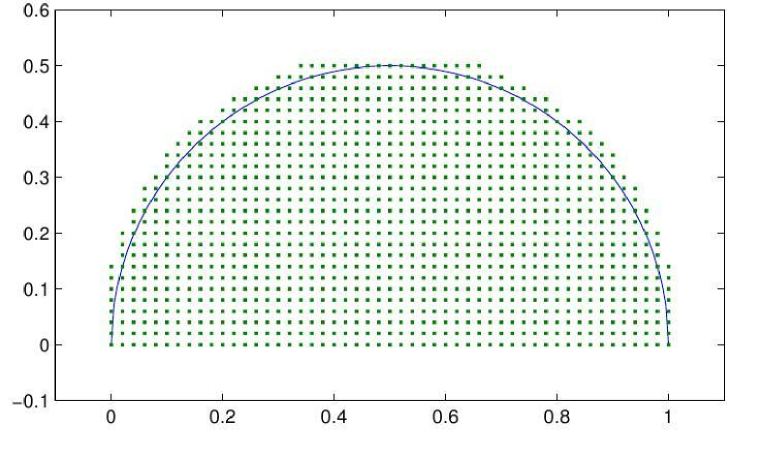
Let $N>0$ be an even integer, $h:=1/N$, and let $D$, $U$, and $H$ be as in Sectionย 3.1. Define $D_{+}=\{(x,y)\in D:y\geq 0\}$. We consider mesh points of the form $(jh,kh)$, where $j\in\mathbb{N}\cup\{0\}$ and $k\in\mathbb{Z}$. Each mesh point $(x_{j},y_{k})=(jh,kh)$ defines a closed mesh square $R_{jk}$ with vertices $(x_{j},y_{k})$, $(x_{j+1},y_{k})$, $(x_{j},y_{k+1})$, and $(x_{j+1},y_{k+1})$. If $D_{h}$ (respectively, $D_{+,h}$) is a finite union of mesh squares and $D_{h}\supset D$ (respectively $D_{+,h}\supset D_{+}$), $D_{h}$ will be called a mesh domain for $D$ (respectively, a mesh domain for $D_{+}$). We could choose $D_{+,h}=[0,1]\times[0,1/2]$, but that choice would add unknowns we do not use. Thus we shall usually take $D_{h}$ (respectively, $D_{+,h}$) to be the union of squares $R_{j,k}$ which have nonempty intersection with the interior of $D$ (respectively, $D_{+})$. The domain $D_{+}$ and a mesh domain $D_{+,h}$ are illustrated in Figureย 3.1.

The mesh domains $D_{h}$ and $D_{+,h}$ correspond to sets $\bar{U}$ and $\bar{H}$ in Sectionย 3.1. If $D$ and $\mathcal{B}$ are symmetric under conjugation or if $\operatorname{Im}(b)\leq-1$ for all $b\in\mathcal{B}$, the observations in Sectionย 3.1 show that we can restrict attention to $D_{+}$ and $D_{+,h}$ instead of the full sets $D$ and $D_{h}$. Indeed, this will be the case for the invariant sets associated to $I_{1}$, $I_{2}$, and $I_{3}$. We also note that in the case $\mathcal{B}=I_{3}$, there is a smaller domain $C\subset D$, symmetric under conjugation, such that $\theta_{b}(C)\subset C\setminus\{0\}$ for $b\in\mathcal{B}$. Although we have not done so, we could have reduced the size of the approximate problem by using a mesh domain $C_{h}$ for $C$.

Refer to caption

Figure 3.1. Domain $D_{+}$ and mesh domain $D_{+,h}$

.

If $D_{h}$ is as above, we take $\bar{U}=D_{h}$ and we assume that $0\leq x\leq 1$ and $|y|<1$ for all $(x,y)\in\bar{U}$. Given a set $\mathcal{B}\subseteq I_{1}$ and s>0๐‘ 0s>0, we assume that s>ฯ„โ€‹(โ„ฌ)๐‘ ๐œโ„ฌs>\tau(\mathcal{B}) (so โˆ‘bโˆˆโ„ฌ(1/|b|2โ€‹s)<โˆžsubscript๐‘โ„ฌ1superscript๐‘2๐‘ \sum_{b\in\mathcal{B}}(1/|b|^{2s})<\infty). If $\mathcal{B}$ is finite, we assume that $R\geq|b|$ for all $b\in\mathcal{B}$ and define Ls:=Ls,R,ฮฑassignsubscript๐ฟ๐‘ subscript๐ฟ๐‘ ๐‘…๐›ผL_{s}:=L_{s,R,\alpha} with $\alpha=0$. If $\mathcal{B}$ is infinite, we assume for the moment that we have found ฮทs,Rโ‰ฅ0subscript๐œ‚๐‘ ๐‘…0\eta_{s,R}\geq 0 and ฮดs,R>0subscript๐›ฟ๐‘ ๐‘…0\delta_{s,R}>0 satisfying (3.8) and (3.9). For ฮฑ=ฮทs,R๐›ผsubscript๐œ‚๐‘ ๐‘…\alpha=\eta_{s,R}, we define Ls,Rโˆ’=Ls,R,ฮฑsubscript๐ฟ๐‘ limit-from๐‘…subscript๐ฟ๐‘ ๐‘…๐›ผL_{s,R-}=L_{s,R,\alpha} and for ฮฑ=ฮดs,R๐›ผsubscript๐›ฟ๐‘ ๐‘…\alpha=\delta_{s,R}, we define Ls,R+=Ls,R,ฮฑsubscript๐ฟ๐‘ limit-from๐‘…subscript๐ฟ๐‘ ๐‘…๐›ผL_{s,R+}=L_{s,R,\alpha} (compare (3.2)); we recall that Theoremย 3.3 implies that

rโ€‹(Ls,Rโˆ’)โ‰คrโ€‹(Ls)โ‰คrโ€‹(Ls,R+).๐‘Ÿsubscript๐ฟ๐‘ limit-from๐‘…๐‘Ÿsubscript๐ฟ๐‘ ๐‘Ÿsubscript๐ฟ๐‘ limit-from๐‘…r(L_{s,R-})\leq r(L_{s})\leq r(L_{s,R+}).

In all cases, we have an operator Ls,R,ฮฑsubscript๐ฟ๐‘ ๐‘…๐›ผL_{s,R,\alpha} where $\alpha\geq 0$ and $R>2$. Theoremย 3.1 implies that Ls,R,ฮฑsubscript๐ฟ๐‘ ๐‘…๐›ผL_{s,R,\alpha} has a unique (to within scalar multiples) strictly positive eigenfunction wssubscript๐‘ค๐‘ w_{s} on $\bar{U}=D_{h}$ which has (assuming $\alpha>0$ or โ„ฌRโ‰ โˆ…subscriptโ„ฌ๐‘…\mathcal{B}_{R}\neq\emptyset) eigenvalue rโ€‹(Ls,R,ฮฑ)>0๐‘Ÿsubscript๐ฟ๐‘ ๐‘…๐›ผ0r(L_{s,R,\alpha})>0. The eigenfunction wssubscript๐‘ค๐‘ w_{s} is $C^{\infty}$ and satisfies (3.3)โ€“(3.7). If $\mathcal{B}$ is symmetric under conjugation, wsโ€‹(zยฏ)=wsโ€‹(z)subscript๐‘ค๐‘ ยฏ๐‘งsubscript๐‘ค๐‘ ๐‘งw_{s}(\bar{z})=w_{s}(z) for all $z\in D_{h}$.

We shall now describe how to find rigorous upper and lower bounds for rโ€‹(Ls,R,ฮฑ)๐‘Ÿsubscript๐ฟ๐‘ ๐‘…๐›ผr(L_{s,R,\alpha}), where $\alpha\geq 0$ or โ„ฌRโ‰ โˆ…subscriptโ„ฌ๐‘…\mathcal{B}_{R}\neq\emptyset. After estimating ฮทs,Rsubscript๐œ‚๐‘ ๐‘…\eta_{s,R} and ฮดs,Rsubscript๐›ฟ๐‘ ๐‘…\delta_{s,R}, this will yield rigorous upper and lower bounds for rโ€‹(Ls)๐‘Ÿsubscript๐ฟ๐‘ r(L_{s}). Our approach is to approximate wssubscript๐‘ค๐‘ w_{s} by a continuous, piecewise bilinear function, i.e., wssubscript๐‘ค๐‘ w_{s} will be bilinear on each mesh square $R_{j,k}$ of the mesh domain $D_{h}$. As noted in Sectionย 3.1, we shall be able to work on $D_{+,h}$ in our particular examples.

More precisely, for fixed $R$ and $\alpha$, our goal is to define nonnegative, square matrices Assubscript๐ด๐‘ A_{s} and Bssubscript๐ต๐‘ B_{s} such that

rโ€‹(As)โ‰คrโ€‹(Ls)โ‰คrโ€‹(Bs),s>ฯ„โ€‹(โ„ฌ).formulae-sequence๐‘Ÿsubscript๐ด๐‘ ๐‘Ÿsubscript๐ฟ๐‘ ๐‘Ÿsubscript๐ต๐‘ ๐‘ ๐œโ„ฌr(A_{s})\leq r(L_{s})\leq r(B_{s}),\quad s>\tau(\mathcal{B}).

If sโˆ—subscript๐‘ s_{*} denotes the unique value of s๐‘ s such that rโ€‹(Lsโˆ—)=ฮปsโˆ—=1๐‘Ÿsubscript๐ฟsubscript๐‘ subscript๐œ†subscript๐‘ 1r(L_{s_{*}})=\lambda_{s_{*}}=1, then sโˆ—subscript๐‘ s_{*} is the Hausdorff dimension of the invariant set associated with $\mathcal{B}$. If we can find a number s1subscript๐‘ 1s_{1} such that rโ€‹(Bs1)โ‰ค1๐‘Ÿsubscript๐ตsubscript๐‘ 11r(B_{s_{1}})\leq 1, then rโ€‹(Ls1)โ‰คrโ€‹(Bs1)โ‰ค1๐‘Ÿsubscript๐ฟsubscript๐‘ 1๐‘Ÿsubscript๐ตsubscript๐‘ 11r(L_{s_{1}})\leq r(B_{s_{1}})\leq 1, and we can conclude that sโˆ—โ‰คs1subscript๐‘ subscript๐‘ 1s_{*}\leq s_{1}. Analogously, if we can find a number s2subscript๐‘ 2s_{2} such that rโ€‹(As2)โ‰ฅ1๐‘Ÿsubscript๐ดsubscript๐‘ 21r(A_{s_{2}})\geq 1, then rโ€‹(Ls2)โ‰ฅrโ€‹(As2)โ‰ฅ1๐‘Ÿsubscript๐ฟsubscript๐‘ 2๐‘Ÿsubscript๐ดsubscript๐‘ 21r(L_{s_{2}})\geq r(A_{s_{2}})\geq 1, and we can conclude that sโˆ—โ‰ฅs2subscript๐‘ subscript๐‘ 2s_{*}\geq s_{2}. By choosing the mesh size $h$ to be sufficiently small, we can make s1โˆ’s2subscript๐‘ 1subscript๐‘ 2s_{1}-s_{2} small, providing a good estimate for sโˆ—subscript๐‘ s_{*}.

Before describing how to construct the matrices Assubscript๐ด๐‘ A_{s} and Bssubscript๐ต๐‘ B_{s}, we need to recall some standard results about bilinear interpolation. On the mesh square

$$R_{k,l}=\{(x,y):x_{k}\leq x\leq x_{k+1},y_{l}\leq y\leq y_{l+1}\},$$

where $x_{k+1}-x_{k}=y_{l+1}-y_{l}=h$, the bilinear interpolant $f^{I}(x,y)$ of a function $f(x,y)$ is given by:

$$f^{I}(x,y)=\Big{[}\frac{x_{k+1}-x}{h}\Big{]}\Big{[}\frac{y_{l+1}-y}{h}\Big{]}f(x_{k},y_{l})+\Big{[}\frac{x-x_{k}}{h}\Big{]}\Big{[}\frac{y_{l+1}-y}{h}\Big{]}f(x_{k+1},y_{l})\\ +\Big{[}\frac{x_{k+1}-x}{h}\Big{]}\Big{[}\frac{y-y_{l}}{h}\Big{]}f(x_{k},y_{l+1})+\Big{[}\frac{x-x_{k}}{h}\Big{]}\Big{[}\frac{y-y_{l}}{h}\Big{]}f(x_{k+1},y_{l+1}).$$

The error in bilinear interpolation satisfies for all $(x,y)\in R_{k,l}$ and some points $(a_{k},b_{l})$ and $(c_{k},d_{l})\in R_{k,l}$,

$$f^{I}(x,y)-f(x,y)=1/2)\Big{[}(x_{k+1}-x)(x-x_{k})(D_{xx}f)(a_{k},b_{l})\\ +(y_{l+1}-y)(y-y_{l})(D_{yy}f)(c_{k},d_{l})\Big{]}.$$

For $z=x+\mathrm{i}y$, let fโ€‹(x,y)=wsโ€‹(ฮธbโ€‹(z))๐‘“๐‘ฅ๐‘ฆsubscript๐‘ค๐‘ subscript๐œƒ๐‘๐‘งf(x,y)=w_{s}(\theta_{b}(z)). Further let $z_{k,l}=x_{k}+\mathrm{i}y_{l}$. If $(\tilde{x},\tilde{y})=(\operatorname{Re}\theta_{b}(z),\operatorname{Im}\theta_{b}(z))\in R_{k,l}$, (which we will sometimes abbreviate by $\theta_{b}(z)\in R_{k,l}$), we get

wsIโ€‹(ฮธbโ€‹(z))=[xk+1โˆ’x~h]โ€‹[yl+1โˆ’y~h]โ€‹wsโ€‹(zk,l)+[x~โˆ’xkh]โ€‹[yl+1โˆ’y~h]โ€‹wsโ€‹(zk+1,l)+[xk+1โˆ’x~h]โ€‹[y~โˆ’ylh]โ€‹wsโ€‹(zk,l+1)+[x~โˆ’xkh]โ€‹[y~โˆ’ylh]โ€‹wsโ€‹(zk+1,l+1).superscriptsubscript๐‘ค๐‘ ๐ผsubscript๐œƒ๐‘๐‘งdelimited-[]subscript๐‘ฅ๐‘˜1~๐‘ฅโ„Ždelimited-[]subscript๐‘ฆ๐‘™1~๐‘ฆโ„Žsubscript๐‘ค๐‘ subscript๐‘ง๐‘˜๐‘™delimited-[]~๐‘ฅsubscript๐‘ฅ๐‘˜โ„Ždelimited-[]subscript๐‘ฆ๐‘™1~๐‘ฆโ„Žsubscript๐‘ค๐‘ subscript๐‘ง๐‘˜1๐‘™delimited-[]subscript๐‘ฅ๐‘˜1~๐‘ฅโ„Ždelimited-[]~๐‘ฆsubscript๐‘ฆ๐‘™โ„Žsubscript๐‘ค๐‘ subscript๐‘ง๐‘˜๐‘™1delimited-[]~๐‘ฅsubscript๐‘ฅ๐‘˜โ„Ždelimited-[]~๐‘ฆsubscript๐‘ฆ๐‘™โ„Žsubscript๐‘ค๐‘ subscript๐‘ง๐‘˜1๐‘™1w_{s}^{I}(\theta_{b}(z))=\Big{[}\frac{x_{k+1}-\tilde{x}}{h}\Big{]}\Big{[}\frac{y_{l+1}-\tilde{y}}{h}\Big{]}w_{s}(z_{k,l})+\Big{[}\frac{\tilde{x}-x_{k}}{h}\Big{]}\Big{[}\frac{y_{l+1}-\tilde{y}}{h}\Big{]}w_{s}(z_{k+1,l})\\ +\Big{[}\frac{x_{k+1}-\tilde{x}}{h}\Big{]}\Big{[}\frac{\tilde{y}-y_{l}}{h}\Big{]}w_{s}(z_{k,l+1})+\Big{[}\frac{\tilde{x}-x_{k}}{h}\Big{]}\Big{[}\frac{\tilde{y}-y_{l}}{h}\Big{]}w_{s}(z_{k+1,l+1}).

Defining

$$\Psi_{b}(z)=1/(\bar{z}+\bar{b}),$$

we have an analogous formula for wsIโ€‹(ฮจbโ€‹(z))superscriptsubscript๐‘ค๐‘ ๐ผsubscriptฮจ๐‘๐‘งw_{s}^{I}(\Psi_{b}(z)), with $(\tilde{x},\tilde{y})=(\operatorname{Re}\Psi_{b}(z),\operatorname{Im}\Psi_{b}(z))$.

We next use inequalities (3.3)โ€“(3.7) to obtain bounds on the interpolation error. By (3.6) and (3.7), we find for $\theta_{b}(z)=\tilde{x}+\mathrm{i}\tilde{y}$, where $(\tilde{x},\tilde{y})\in R_{k,l}$,

โˆ’[s8โ€‹ฮณ2โ€‹(s+1)+sฮณ2]โ€‹([xk+1โˆ’x~]โ€‹[x~โˆ’xk]โ€‹wsโ€‹(ak,bl)+[yl+1โˆ’y~]โ€‹[y~โˆ’yl]โ€‹wsโ€‹(ck,dl))โ‰คwsIโ€‹(ฮธbโ€‹(z))โˆ’wsโ€‹(ฮธbโ€‹(z))โ‰คsโ€‹(2โ€‹s+1)ฮณ2โ€‹([xk+1โˆ’x~]โ€‹[x~โˆ’xk]โ€‹wsโ€‹(ak,bl)+[yl+1โˆ’y~]โ€‹[y~โˆ’yl]โ€‹wsโ€‹(ck,dl)).delimited-[]๐‘ 8superscript๐›พ2๐‘ 1๐‘ superscript๐›พ2delimited-[]subscript๐‘ฅ๐‘˜1~๐‘ฅdelimited-[]~๐‘ฅsubscript๐‘ฅ๐‘˜subscript๐‘ค๐‘ subscript๐‘Ž๐‘˜subscript๐‘๐‘™delimited-[]subscript๐‘ฆ๐‘™1~๐‘ฆdelimited-[]~๐‘ฆsubscript๐‘ฆ๐‘™subscript๐‘ค๐‘ subscript๐‘๐‘˜subscript๐‘‘๐‘™superscriptsubscript๐‘ค๐‘ ๐ผsubscript๐œƒ๐‘๐‘งsubscript๐‘ค๐‘ subscript๐œƒ๐‘๐‘ง๐‘ 2๐‘ 1superscript๐›พ2delimited-[]subscript๐‘ฅ๐‘˜1~๐‘ฅdelimited-[]~๐‘ฅsubscript๐‘ฅ๐‘˜subscript๐‘ค๐‘ subscript๐‘Ž๐‘˜subscript๐‘๐‘™delimited-[]subscript๐‘ฆ๐‘™1~๐‘ฆdelimited-[]~๐‘ฆsubscript๐‘ฆ๐‘™subscript๐‘ค๐‘ subscript๐‘๐‘˜subscript๐‘‘๐‘™-\Big{[}\frac{s}{8\gamma^{2}(s+1)}+\frac{s}{\gamma^{2}}\Big{]}\left([x_{k+1}-\tilde{x}][\tilde{x}-x_{k}]w_{s}(a_{k},b_{l})+[y_{l+1}-\tilde{y}][\tilde{y}-y_{l}]w_{s}(c_{k},d_{l})\right)\\ \leq w_{s}^{I}(\theta_{b}(z))-w_{s}(\theta_{b}(z))\\ \leq\frac{s(2s+1)}{\gamma^{2}}\left([x_{k+1}-\tilde{x}][\tilde{x}-x_{k}]w_{s}(a_{k},b_{l})+[y_{l+1}-\tilde{y}][\tilde{y}-y_{l}]w_{s}(c_{k},d_{l})\right).

Applying (3.3), we then obtain

โˆ’sฮณ2โ€‹[9+8โ€‹s8โ€‹(s+1)]โ€‹([xk+1โˆ’x~]โ€‹[x~โˆ’xk]+[yl+1โˆ’y~]โ€‹[y~โˆ’yl])โ€‹expโก(10โ€‹sโ€‹hฮณ)โ€‹wsIโ€‹(ฮธbโ€‹(z))โ‰คwsIโ€‹(ฮธbโ€‹(z))โˆ’wsโ€‹(ฮธbโ€‹(z))โ‰คsโ€‹(2โ€‹s+1)ฮณ2โ€‹([xk+1โˆ’x~]โ€‹[x~โˆ’xk]+[yl+1โˆ’y~]โ€‹[y~โˆ’yl])โ€‹expโก(10โ€‹sโ€‹hฮณ)โ€‹wsIโ€‹(ฮธbโ€‹(z)).๐‘ superscript๐›พ2delimited-[]98๐‘ 8๐‘ 1delimited-[]subscript๐‘ฅ๐‘˜1~๐‘ฅdelimited-[]~๐‘ฅsubscript๐‘ฅ๐‘˜delimited-[]subscript๐‘ฆ๐‘™1~๐‘ฆdelimited-[]~๐‘ฆsubscript๐‘ฆ๐‘™10๐‘ โ„Ž๐›พsuperscriptsubscript๐‘ค๐‘ ๐ผsubscript๐œƒ๐‘๐‘งsuperscriptsubscript๐‘ค๐‘ ๐ผsubscript๐œƒ๐‘๐‘งsubscript๐‘ค๐‘ subscript๐œƒ๐‘๐‘ง๐‘ 2๐‘ 1superscript๐›พ2delimited-[]subscript๐‘ฅ๐‘˜1~๐‘ฅdelimited-[]~๐‘ฅsubscript๐‘ฅ๐‘˜delimited-[]subscript๐‘ฆ๐‘™1~๐‘ฆdelimited-[]~๐‘ฆsubscript๐‘ฆ๐‘™10๐‘ โ„Ž๐›พsuperscriptsubscript๐‘ค๐‘ ๐ผsubscript๐œƒ๐‘๐‘ง-\frac{s}{\gamma^{2}}\Big{[}\frac{9+8s}{8(s+1)}\Big{]}\left([x_{k+1}-\tilde{x}][\tilde{x}-x_{k}]+[y_{l+1}-\tilde{y}][\tilde{y}-y_{l}]\right)\exp\big{(}\frac{\sqrt{10}sh}{\gamma}\big{)}w_{s}^{I}(\theta_{b}(z))\\ \leq w_{s}^{I}(\theta_{b}(z))-w_{s}(\theta_{b}(z))\\ \leq\frac{s(2s+1)}{\gamma^{2}}\left([x_{k+1}-\tilde{x}][\tilde{x}-x_{k}]+[y_{l+1}-\tilde{y}][\tilde{y}-y_{l}]\right)\exp\big{(}\frac{\sqrt{10}sh}{\gamma}\big{)}w_{s}^{I}(\theta_{b}(z)).

since any point in $R_{k,l}$ is within $\sqrt{2}h$ of each of the four corners of the square $R_{k,l}$. An analogous result holds for wsโ€‹(ฮจbโ€‹(z))subscript๐‘ค๐‘ subscriptฮจ๐‘๐‘งw_{s}(\Psi_{b}(z)).

Using this estimate, we have precise upper and lower bounds on the error in the mesh square $R_{k,l}$ that only depend on the function values of wssubscript๐‘ค๐‘ w_{s} at the four corners of the square and the value of $b$. Letting

$\displaystyle\operatorname{err}_{b}^{1}(\theta_{b}(z))$ =([xk+1โˆ’x~]โ€‹[x~โˆ’xk]+[yl+1โˆ’y~]โ€‹[y~โˆ’yl])โ€‹sโ€‹(2โ€‹s+1)ฮณ2โ€‹expโก(10โ€‹sโ€‹h/ฮณ),absentdelimited-[]subscript๐‘ฅ๐‘˜1~๐‘ฅdelimited-[]~๐‘ฅsubscript๐‘ฅ๐‘˜delimited-[]subscript๐‘ฆ๐‘™1~๐‘ฆdelimited-[]~๐‘ฆsubscript๐‘ฆ๐‘™๐‘ 2๐‘ 1superscript๐›พ210๐‘ โ„Ž๐›พ\displaystyle=\Big{(}[x_{k+1}-\tilde{x}][\tilde{x}-x_{k}]+[y_{l+1}-\tilde{y}][\tilde{y}-y_{l}]\Big{)}\frac{s(2s+1)}{\gamma^{2}}\exp(\sqrt{10}sh/\gamma),
$\displaystyle\operatorname{err}_{b}^{2}(\theta_{b}(z))$ =([xk+1โˆ’x~]โ€‹[x~โˆ’xk]+[yl+1โˆ’y~]โ€‹[y~โˆ’yl])โ€‹sฮณ2โ€‹[9+8โ€‹s8+8โ€‹s]โ€‹expโก(10โ€‹sโ€‹h/ฮณ),absentdelimited-[]subscript๐‘ฅ๐‘˜1~๐‘ฅdelimited-[]~๐‘ฅsubscript๐‘ฅ๐‘˜delimited-[]subscript๐‘ฆ๐‘™1~๐‘ฆdelimited-[]~๐‘ฆsubscript๐‘ฆ๐‘™๐‘ superscript๐›พ2delimited-[]98๐‘ 88๐‘ 10๐‘ โ„Ž๐›พ\displaystyle=\Big{(}[x_{k+1}-\tilde{x}][\tilde{x}-x_{k}]+[y_{l+1}-\tilde{y}][\tilde{y}-y_{l}]\Big{)}\frac{s}{\gamma^{2}}\Big{[}\frac{9+8s}{8+8s}\Big{]}\exp(\sqrt{10}sh/\gamma),

(where again $\theta_{b}(z)=\tilde{x}+\mathrm{i}\tilde{y}$), we have for each mesh point $z_{i,j}=x_{i}+\mathrm{i}y_{j}$, with $\theta_{b}(z_{i,j})\in R_{k,l}$,

[1โˆ’errb1โก(zi,j)]โ€‹wsIโ€‹(ฮธbโ€‹(zi,j))โ‰คwsโ€‹(ฮธbโ€‹(zi,j))โ‰ค[1+errb2โก(zi,j)]โ€‹wsIโ€‹(ฮธbโ€‹(zi,j)).delimited-[]1superscriptsubscripterr๐‘1subscript๐‘ง๐‘–๐‘—superscriptsubscript๐‘ค๐‘ ๐ผsubscript๐œƒ๐‘subscript๐‘ง๐‘–๐‘—subscript๐‘ค๐‘ subscript๐œƒ๐‘subscript๐‘ง๐‘–๐‘—delimited-[]1superscriptsubscripterr๐‘2subscript๐‘ง๐‘–๐‘—superscriptsubscript๐‘ค๐‘ ๐ผsubscript๐œƒ๐‘subscript๐‘ง๐‘–๐‘—[1-\operatorname{err}_{b}^{1}(z_{i,j})]w_{s}^{I}(\theta_{b}(z_{i,j}))\leq w_{s}(\theta_{b}(z_{i,j}))\leq[1+\operatorname{err}_{b}^{2}(z_{i,j})]w_{s}^{I}(\theta_{b}(z_{i,j})).

Again, the analogous result holds for wsโ€‹(ฮจbโ€‹(z))subscript๐‘ค๐‘ subscriptฮจ๐‘๐‘งw_{s}(\Psi_{b}(z)).

To obtain the upper and lower matrices, we first note that for each mesh point $z_{i,j}$,

ฮฑโ€‹wsโ€‹(0)+โˆ‘bโˆˆโ„ฌR1|zi,j+b|2โ€‹sโ€‹[1โˆ’errb1โก(zi,j)]โ€‹wsIโ€‹(ฮธbโ€‹(zi,j))โ‰คโˆ‘bโˆˆโ„ฌR1|zi,j+b|2โ€‹sโ€‹wsโ€‹(ฮธbโ€‹(zi,j))+ฮฑโ€‹wsโ€‹(0)โ‰คโˆ‘bโˆˆโ„ฌR1|zi,j+b|2โ€‹sโ€‹[1+errb2โก(zi,j)]โ€‹wsIโ€‹(ฮธbโ€‹(zi,j))+ฮฑโ€‹wsโ€‹(0).๐›ผsubscript๐‘ค๐‘ 0subscript๐‘subscriptโ„ฌ๐‘…1superscriptsubscript๐‘ง๐‘–๐‘—๐‘2๐‘ delimited-[]1superscriptsubscripterr๐‘1subscript๐‘ง๐‘–๐‘—superscriptsubscript๐‘ค๐‘ ๐ผsubscript๐œƒ๐‘subscript๐‘ง๐‘–๐‘—subscript๐‘subscriptโ„ฌ๐‘…1superscriptsubscript๐‘ง๐‘–๐‘—๐‘2๐‘ subscript๐‘ค๐‘ subscript๐œƒ๐‘subscript๐‘ง๐‘–๐‘—๐›ผsubscript๐‘ค๐‘ 0subscript๐‘subscriptโ„ฌ๐‘…1superscriptsubscript๐‘ง๐‘–๐‘—๐‘2๐‘ delimited-[]1superscriptsubscripterr๐‘2subscript๐‘ง๐‘–๐‘—superscriptsubscript๐‘ค๐‘ ๐ผsubscript๐œƒ๐‘subscript๐‘ง๐‘–๐‘—๐›ผsubscript๐‘ค๐‘ 0\alpha w_{s}(0)+\sum_{b\in\mathcal{B}_{R}}\frac{1}{|z_{i,j}+b|^{2s}}[1-\operatorname{err}_{b}^{1}(z_{i,j})]w_{s}^{I}(\theta_{b}(z_{i,j}))\\ \leq\sum_{b\in\mathcal{B}_{R}}\frac{1}{|z_{i,j}+b|^{2s}}w_{s}(\theta_{b}(z_{i,j}))+\alpha w_{s}(0)\\ \leq\sum_{b\in\mathcal{B}_{R}}\frac{1}{|z_{i,j}+b|^{2s}}[1+\operatorname{err}_{b}^{2}(z_{i,j})]w_{s}^{I}(\theta_{b}(z_{i,j}))+\alpha w_{s}(0).

Motivated by the above inequality, we now define matrices Assubscript๐ด๐‘ A_{s} and Bssubscript๐ต๐‘ B_{s} which have nonnegative entries and satisfy the property that rโ€‹(As)โ‰คrโ€‹(Ls)โ‰คrโ€‹(Bs)๐‘Ÿsubscript๐ด๐‘ ๐‘Ÿsubscript๐ฟ๐‘ ๐‘Ÿsubscript๐ต๐‘ r(A_{s})\leq r(L_{s})\leq r(B_{s}). For clarity, we do this in several steps. For $f$ a continuous, piecewise bilinear function defined on the mesh domain $D_{h}$, we first define operators ๐‘จssubscript๐‘จ๐‘ \boldsymbol{A}_{s} and ๐‘ฉssubscript๐‘ฉ๐‘ \boldsymbol{B}_{s} (which also depend on $\alpha$) by:

(3.10) (๐‘จsโ€‹f)โ€‹(zi,j)subscript๐‘จ๐‘ ๐‘“subscript๐‘ง๐‘–๐‘—\displaystyle(\boldsymbol{A}_{s}f)(z_{i,j}) =โˆ‘bโˆˆโ„ฌR1|zi,j+b|2โ€‹sโ€‹[1โˆ’errb1โก(zi,j)]โ€‹fโ€‹(ฮธbโ€‹(zi,j))+ฮฑโ€‹fโ€‹(0),absentsubscript๐‘subscriptโ„ฌ๐‘…1superscriptsubscript๐‘ง๐‘–๐‘—๐‘2๐‘ delimited-[]1superscriptsubscripterr๐‘1subscript๐‘ง๐‘–๐‘—๐‘“subscript๐œƒ๐‘subscript๐‘ง๐‘–๐‘—๐›ผ๐‘“0\displaystyle=\sum_{b\in\mathcal{B}_{R}}\frac{1}{|z_{i,j}+b|^{2s}}[1-\operatorname{err}_{b}^{1}(z_{i,j})]f(\theta_{b}(z_{i,j}))+\alpha f(0),
(3.11) (๐‘ฉsโ€‹f)โ€‹(zi,j)subscript๐‘ฉ๐‘ ๐‘“subscript๐‘ง๐‘–๐‘—\displaystyle(\boldsymbol{B}_{s}f)(z_{i,j}) =โˆ‘bโˆˆโ„ฌR1|zi,j+b|2โ€‹sโ€‹[1+errb2โก(zi,j)]โ€‹fโ€‹(ฮธbโ€‹(zi,j))+ฮฑโ€‹fโ€‹(0),absentsubscript๐‘subscriptโ„ฌ๐‘…1superscriptsubscript๐‘ง๐‘–๐‘—๐‘2๐‘ delimited-[]1superscriptsubscripterr๐‘2subscript๐‘ง๐‘–๐‘—๐‘“subscript๐œƒ๐‘subscript๐‘ง๐‘–๐‘—๐›ผ๐‘“0\displaystyle=\sum_{b\in\mathcal{B}_{R}}\frac{1}{|z_{i,j}+b|^{2s}}[1+\operatorname{err}_{b}^{2}(z_{i,j})]f(\theta_{b}(z_{i,j}))+\alpha f(0),

where $z_{i,j}$ is a mesh point in $D_{h}$. In the above, if $(\tilde{x},\tilde{y})=(\operatorname{Re}\theta_{b}(z),\operatorname{Im}\theta_{b}(z))\in R_{k,l}$, then, using bilinearity,

(3.12) $$f(\theta_{b}(z))=\Big{[}\frac{x_{k+1}-\tilde{x}}{h}\Big{]}\Big{[}\frac{y_{l+1}-\tilde{y}}{h}\Big{]}f(z_{k,l})+\Big{[}\frac{\tilde{x}-x_{k}}{h}\Big{]}\Big{[}\frac{y_{l+1}-\tilde{y}}{h}\Big{]}f(z_{k+1,l})\\ +\Big{[}\frac{x_{k+1}-\tilde{x}}{h}\Big{]}\Big{[}\frac{\tilde{y}-y_{l}}{h}\Big{]}f(z_{k,l+1})+\Big{[}\frac{\tilde{x}-x_{k}}{h}\Big{]}\Big{[}\frac{\tilde{y}-y_{l}}{h}\Big{]}f(z_{k+1,l+1}).$$

Let $Q=\{z_{i,j}:z_{i,j}\text{ is a mesh point of }D_{h}\}$ and consider the finite dimensional vector space $C_{\mathbb{R}}(Q)$. We can consider $f$ above as an element of $C_{\mathbb{R}}(Q)$, where $f(\theta_{b}(z))$ is defined by (3.12). If we use (3.12) in (3.10) and (3.11), ๐‘จssubscript๐‘จ๐‘ \boldsymbol{A}_{s} and ๐‘ฉssubscript๐‘ฉ๐‘ \boldsymbol{B}_{s} define linear maps of $C_{\mathbb{R}}(Q)$ to $C_{\mathbb{R}}(Q)$. Note that since $\operatorname{err}_{b}^{i}=O(h^{2})$ for $i=1,2$, ๐‘จsโ€‹(S+)โŠ‚S+subscript๐‘จ๐‘ limit-from๐‘†limit-from๐‘†\boldsymbol{A}_{s}(S+)\subset S+ and ๐‘ฉsโ€‹(S+)โŠ‚S+subscript๐‘ฉ๐‘ limit-from๐‘†limit-from๐‘†\boldsymbol{B}_{s}(S+)\subset S+ for $h$ sufficiently small, where $S+$ denotes the set of nonnegative functions in $C_{\mathbb{R}}(Q)$. If, for fixed $\alpha\geq 0$, we take f=ws๐‘“subscript๐‘ค๐‘ f=w_{s}, the strictly positive eigenfunction of Ls,R,ฮฑsubscript๐ฟ๐‘ ๐‘…๐›ผL_{s,R,\alpha}, our construction insures that for all mesh points $z_{i,j}\in D_{h}$,

(๐‘จsโ€‹ws)โ€‹(zi,j)โ‰ค(Ls,R,ฮฑโ€‹ws)โ€‹(zi,j)=rโ€‹(Ls,R,ฮฑ)โ€‹wsโ€‹(zi,j)โ‰ค(๐‘ฉsโ€‹ws)โ€‹(zi,j).subscript๐‘จ๐‘ subscript๐‘ค๐‘ subscript๐‘ง๐‘–๐‘—subscript๐ฟ๐‘ ๐‘…๐›ผsubscript๐‘ค๐‘ subscript๐‘ง๐‘–๐‘—๐‘Ÿsubscript๐ฟ๐‘ ๐‘…๐›ผsubscript๐‘ค๐‘ subscript๐‘ง๐‘–๐‘—subscript๐‘ฉ๐‘ subscript๐‘ค๐‘ subscript๐‘ง๐‘–๐‘—(\boldsymbol{A}_{s}w_{s})(z_{i,j})\leq(L_{s,R,\alpha}w_{s})(z_{i,j})=r(L_{s,R,\alpha})w_{s}(z_{i,j})\leq(\boldsymbol{B}_{s}w_{s})(z_{i,j}).

Lemmaย 2.2 now implies that

(3.13) rโ€‹(๐‘จs)โ‰คrโ€‹(Ls,R,ฮฑ)โ‰คrโ€‹(๐‘ฉs).๐‘Ÿsubscript๐‘จ๐‘ ๐‘Ÿsubscript๐ฟ๐‘ ๐‘…๐›ผ๐‘Ÿsubscript๐‘ฉ๐‘ r(\boldsymbol{A}_{s})\leq r(L_{s,R,\alpha})\leq r(\boldsymbol{B}_{s}).

If $\mathcal{B}$ is finite, so $\alpha=0$ and Ls,R=Lssubscript๐ฟ๐‘ ๐‘…subscript๐ฟ๐‘ L_{s,R}=L_{s}, (3.13) gives an estimate for rโ€‹(Ls)๐‘Ÿsubscript๐ฟ๐‘ r(L_{s}) in terms of the spectral radii of finite dimensional linear maps ๐‘จssubscript๐‘จ๐‘ \boldsymbol{A}_{s} and ๐‘ฉssubscript๐‘ฉ๐‘ \boldsymbol{B}_{s}. If $\mathcal{B}$ is infinite and $R>0$ has been chosen and ฮทs,Rsubscript๐œ‚๐‘ ๐‘…\eta_{s,R} and ฮดs,Rsubscript๐›ฟ๐‘ ๐‘…\delta_{s,R} have been estimated as in Theoremsย 5.12 and 5.13, we take ฮฑ=ฮทs,R๐›ผsubscript๐œ‚๐‘ ๐‘…\alpha=\eta_{s,R} in (3.10) and define ๐‘จssubscript๐‘จ๐‘ \boldsymbol{A}_{s} as in (3.10) and we obtain, using Theoremย 3.3,

(3.14) rโ€‹(๐‘จs)โ‰คrโ€‹(Ls,Rโˆ’)โ‰คrโ€‹(Ls).๐‘Ÿsubscript๐‘จ๐‘ ๐‘Ÿsubscript๐ฟ๐‘ limit-from๐‘…๐‘Ÿsubscript๐ฟ๐‘ r(\boldsymbol{A}_{s})\leq r(L_{s,R-})\leq r(L_{s}).

Taking ฮฑ=ฮดs,R๐›ผsubscript๐›ฟ๐‘ ๐‘…\alpha=\delta_{s,R} in (3.11), we define ๐‘ฉssubscript๐‘ฉ๐‘ \boldsymbol{B}_{s} as in (3.11) to obtain

(3.15) rโ€‹(Ls)โ‰คrโ€‹(Ls,R+)โ‰คrโ€‹(๐‘ฉs).๐‘Ÿsubscript๐ฟ๐‘ ๐‘Ÿsubscript๐ฟ๐‘ limit-from๐‘…๐‘Ÿsubscript๐‘ฉ๐‘ r(L_{s})\leq r(L_{s,R+})\leq r(\boldsymbol{B}_{s}).

As a practical matter, it remains to describe the linear maps ๐‘จssubscript๐‘จ๐‘ \boldsymbol{A}_{s} and ๐‘ฉssubscript๐‘ฉ๐‘ \boldsymbol{B}_{s} as matrices. For simplicity, we totally order the elements of $Q$ by the dictionary ordering, i.e., $z_{i,j}<z_{p,q}$ if and only if $i<p$ or if $i=p$ and $j<q$. Then we can identify $f\in C_{\mathbb{R}}(Q)$ with a column vector $(f_{1},\ldots,f_{k},\ldots,f_{n})^{T}$, where $f(z_{i,j}):=f_{k}$ if $z_{i,j}$ is the $k$th element when the mesh points in $D_{h}$ are ordered as above and $n$ is the total number of mesh points in $D_{h}$, Since $f(\theta_{b}(z))$ is a linear combination of four components of $f$, the mesh point $z_{i,j}$ will produce row $k$ of the matrix Assubscript๐ด๐‘ A_{s} (and similarly for Bssubscript๐ต๐‘ B_{s}). A more detailed description of this procedure can be found in [11] for a simpler one dimensional problem. Since Assubscript๐ด๐‘ A_{s} and Bssubscript๐ต๐‘ B_{s} are just representations of the linear maps ๐‘จssubscript๐‘จ๐‘ \boldsymbol{A}_{s} and ๐‘ฉssubscript๐‘ฉ๐‘ \boldsymbol{B}_{s}, we can replace rโ€‹(๐‘จs)๐‘Ÿsubscript๐‘จ๐‘ r(\boldsymbol{A}_{s}) by rโ€‹(As)๐‘Ÿsubscript๐ด๐‘ r(A_{s}) in (3.14) and rโ€‹(๐‘ฉs)๐‘Ÿsubscript๐‘ฉ๐‘ r(\boldsymbol{B}_{s}) by rโ€‹(Bs)๐‘Ÿsubscript๐ต๐‘ r(B_{s}) in (3.15). Thus, we can restate (3.14) and (3.15) in terms of the spectral radii of the matrices Assubscript๐ด๐‘ A_{s} and Bssubscript๐ต๐‘ B_{s}, which better conforms to the description in Sectionย 1:

rโ€‹(As)โ‰คrโ€‹(Ls)โ‰คrโ€‹(Bs).๐‘Ÿsubscript๐ด๐‘ ๐‘Ÿsubscript๐ฟ๐‘ ๐‘Ÿsubscript๐ต๐‘ r(A_{s})\leq r(L_{s})\leq r(B_{s}).

As described in Sectionย 1, if sโˆ—subscript๐‘ s_{*} denotes the unique value of s๐‘ s such that rโ€‹(Lsโˆ—)=ฮปsโˆ—=1๐‘Ÿsubscript๐ฟsubscript๐‘ subscript๐œ†subscript๐‘ 1r(L_{s_{*}})=\lambda_{s_{*}}=1, then sโˆ—subscript๐‘ s_{*} is the Hausdorff dimension of the invariant set under study. Hence, if we can find a number s1subscript๐‘ 1s_{1} such that rโ€‹(Bs1)โ‰ค1๐‘Ÿsubscript๐ตsubscript๐‘ 11r(B_{s_{1}})\leq 1, then rโ€‹(Ls1)โ‰คrโ€‹(Bs1)โ‰ค1๐‘Ÿsubscript๐ฟsubscript๐‘ 1๐‘Ÿsubscript๐ตsubscript๐‘ 11r(L_{s_{1}})\leq r(B_{s_{1}})\leq 1, and we can conclude that sโˆ—โ‰คs1subscript๐‘ subscript๐‘ 1s_{*}\leq s_{1}. Analogously, if we can find a number s2subscript๐‘ 2s_{2} such that rโ€‹(As2)โ‰ฅ1๐‘Ÿsubscript๐ดsubscript๐‘ 21r(A_{s_{2}})\geq 1, then rโ€‹(Ls2)โ‰ฅrโ€‹(As2)โ‰ฅ1๐‘Ÿsubscript๐ฟsubscript๐‘ 2๐‘Ÿsubscript๐ดsubscript๐‘ 21r(L_{s_{2}})\geq r(A_{s_{2}})\geq 1, and we can conclude that sโˆ—โ‰ฅs2subscript๐‘ subscript๐‘ 2s_{*}\geq s_{2}. By choosing the mesh sufficiently fine and both rโ€‹(Bs1)๐‘Ÿsubscript๐ตsubscript๐‘ 1r(B_{s_{1}}) and rโ€‹(As2)๐‘Ÿsubscript๐ดsubscript๐‘ 2r(A_{s_{2}}) very close to one, we can make s1โˆ’s2subscript๐‘ 1subscript๐‘ 2s_{1}-s_{2} small, providing a good estimate for sโˆ—subscript๐‘ s_{*}. As noted in Sectionย 1, since the map sโ†ฆrโ€‹(Ls,R,ฮฑ)maps-to๐‘ ๐‘Ÿsubscript๐ฟ๐‘ ๐‘…๐›ผs\mapsto r(L_{s,R,\alpha}) is log convex, we can find the desired values of s1subscript๐‘ 1s_{1} and s2subscript๐‘ 2s_{2} by using a slight modification of the secant method applied to finding zeros of the functions logโก[rโ€‹(As2)]๐‘Ÿsubscript๐ดsubscript๐‘ 2\log[r(A_{s_{2}})] and logโก[rโ€‹(Bs2)]๐‘Ÿsubscript๐ตsubscript๐‘ 2\log[r(B_{s_{2}})]. We also note that since the matrices Assubscript๐ด๐‘ A_{s} and Bssubscript๐ต๐‘ B_{s} will have a single dominant eigenvalue, (see Sectionย 6 of this paper and Section 7 of [11]), the spectral radius is easily computed by a variant of the power method (in fact, our computer codes simply call the Matlab routine eigs). Indeed, the same program also gives high order approximations to the strictly positive eigenvectors associated to rโ€‹(As)๐‘Ÿsubscript๐ด๐‘ r(A_{s}) and rโ€‹(Bs)๐‘Ÿsubscript๐ต๐‘ r(B_{s}).

By our remarks above, it only remains to use our estimates for ฮทs,Rsubscript๐œ‚๐‘ ๐‘…\eta_{s,R} and ฮดs,Rsubscript๐›ฟ๐‘ ๐‘…\delta_{s,R} in (3.8) and (3.9) when $\mathcal{B}$ is infinite, since then we will have the matrices Assubscript๐ด๐‘ A_{s} and Bssubscript๐ต๐‘ B_{s}.

In Tableย 3.1, we present the computation of upper and lower bounds for the Hausdorff dimension of the invariant sets associated to $\mathcal{B}=I_{1},I_{2}$, and $I_{3}$. In the table, we study the effects of decreasing the mesh size $h$ and increasing the value of $R$, which corresponds to only including terms in the sum for which $|b|\leq R$. Each row in the table gives upper and lower bounds, and for $R$ fixed, one can see that the lower bounds are increasing and the upper bounds decreasing as $h$ is decreased. Similarly, taking a larger value of $R$ improves the bounds for the same mesh size. Except for possible round off error in these calculations, which we do not expect to affect the results for the number of decimal places shown, our theorems prove that these are in fact upper and lower bounds for the actual Hausdorff dimension.

Table 3.1. Computation of Hausdorff dimension s๐‘ s for several values of $h$ and $R$ (rounded to 5 decimal places).
Set $h$ $R$ lower s๐‘ s upper s๐‘ s
$I_{1}$ $.02$ $100$ 1.85516 1.85608
$I_{1}$ $.01$ $100$ 1.85563 1.85594
$I_{1}$ $.005$ $100$ 1.85574 1.85590
$I_{1}$ $.02$ $200$ 1.85521 1.85604
$I_{1}$ $.01$ $200$ 1.85568 1.85589
$I_{1}$ $.02$ $300$ 1.85522 1.85603
$I_{2}$ $.02$ $100$ 1.48883 1.49010
$I_{2}$ $.01$ $100$ 1.48904 1.49003
$I_{2}$ $.005$ $100$ 1.48909 1.49002
$I_{2}$ $.02$ $200$ 1.48925 1.48985
$I_{2}$ $.01$ $200$ 1.48946 1.48978
$I_{2}$ $.02$ $300$ 1.48933 1.48981
$I_{3}$ $.02$ 1.53706 1.53790
$I_{3}$ $.01$ 1.53754 1.53774
$I_{3}$ $.005$ 1.53765 1.53770
Remark 3.1.

It is important to note that, given s1subscript๐‘ 1s_{1} and s2subscript๐‘ 2s_{2}, Bs1subscript๐ตsubscript๐‘ 1B_{s_{1}} and As2subscript๐ดsubscript๐‘ 2A_{s_{2}} are, modulo roundoff errors in computation, known exactly. Furthermore, our computer program furnishes (purported) strictly positive eigenvectors ws1subscript๐‘คsubscript๐‘ 1w_{s_{1}} for Bs1subscript๐ตsubscript๐‘ 1B_{s_{1}} and us2subscript๐‘ขsubscript๐‘ 2u_{s_{2}} for As2subscript๐ดsubscript๐‘ 2A_{s_{2}}, with respective eigenvalues rโ€‹(Bs1)<1๐‘Ÿsubscript๐ตsubscript๐‘ 11r(B_{s_{1}})<1 and rโ€‹(As2)>1๐‘Ÿsubscript๐ดsubscript๐‘ 21r(A_{s_{2}})>1. However, we do not need to know whether ws1subscript๐‘คsubscript๐‘ 1w_{s_{1}} and us2subscript๐‘ขsubscript๐‘ 2u_{s_{2}} are actually eigenvectors. It suffices to verify that

(3.16) Bs1โ€‹ws1โ‰คws1andAs2โ€‹us2โ‰ฅus2,formulae-sequencesubscript๐ตsubscript๐‘ 1subscript๐‘คsubscript๐‘ 1subscript๐‘คsubscript๐‘ 1andsubscript๐ดsubscript๐‘ 2subscript๐‘ขsubscript๐‘ 2subscript๐‘ขsubscript๐‘ 2B_{s_{1}}w_{s_{1}}\leq w_{s_{1}}\qquad\text{and}\qquad A_{s_{2}}u_{s_{2}}\geq u_{s_{2}},

since then Lemmaย 2.2 implies that rโ€‹(Bs1)โ‰ค1๐‘Ÿsubscript๐ตsubscript๐‘ 11r(B_{s_{1}})\leq 1 and rโ€‹(As2)โ‰ฅ1๐‘Ÿsubscript๐ดsubscript๐‘ 21r(A_{s_{2}})\geq 1, and we obtain that s2โ‰คsโˆ—โ‰คs1subscript๐‘ 2subscript๐‘ subscript๐‘ 1s_{2}\leq s_{*}\leq s_{1}. The vectors us2subscript๐‘ขsubscript๐‘ 2u_{s_{2}} and ws1subscript๐‘คsubscript๐‘ 1w_{s_{1}} are given to us exactly by the program. We have verified (3.16) to high accuracy, but we have not used interval arithmetic. If we had used interval arithmetic to calculate Bs1subscript๐ตsubscript๐‘ 1B_{s_{1}}, As2subscript๐ดsubscript๐‘ 2A_{s_{2}}, and to verify (3.16), the estimates in Tableย 3.1 would be completely rigorous. It is in that sense that we list the following result as a theorem.

Theorem 3.5.

The Hausdorff dimensions of the invariant sets associated to $\mathcal{B}=I_{1}$, $I_{2}$, and $I_{3}$ satisfy the bounds

$$\displaystyle I_{1}:\quad 1.85574\leq s\leq 1.85589,\qquad I_{2}:\quad 1.48946\leq s\leq 1.48978,$$
$$\displaystyle I_{3}:\quad 1.53765\leq s\leq 1.53770.$$

3.3. Higher order approximation

Although the theory developed in this paper does not apply to higher order piecewise polynomial approximation, since one cannot guarantee that the approximate matrices have nonnegative entries, we also report in Tableย 3.2 and Tableย 3.3 the results of higher order piecewise polynomial approximation to demonstrate the promise of this approach. In this case, we only provide the results for the approximate matrix, which does not contain any corrections for the interpolation error.

Since we did not have an exact solution for the problem corresponding to the set $I_{3}$, we cannot compare the actual errors. However, assuming the last entry in Tableย 3.2 gives the most accurate approximation, we see that the third entry using piecewise cubics is accurate to 10 decimal places, which is a significant improvement over the last entry for linear approximation, which only produces 5 correct digits after the decimal point. This is consistent with the theory of approximation of smooth functions by piecewise polynomials, which shows that the convergence rate grows as the degree of the polynomials is increased. In the computations shown using higher order piecewise polynomials, to get a fair comparison, we have adjusted the mesh sizes so that the results for different degree piecewise polynomials will have approximately the same number of degrees of freedom (DOF).

Table 3.2. Computation of Hausdorff dimension s๐‘ s of the set $I_{3}$ using higher order piecewise polynomials.
degree h # DOF s๐‘ s
1 .02 1098 1.537729111247678
1 .01 4165 1.537694920731214
1 .005 16201 1.537686565250360
2 0.041667 1041 1.537683708302400
2 0.020833 3913 1.537683729607203
2 0.010417 15089 1.537683732415111
3 0.0625 1081 1.537683753797206
3 0.03125 3997 1.537683734167568
3 0.015625 15283 1.537683732983929
3 0.0078125 59545 1.537683732912027

In a future paper we hope to prove that rigorous upper and lower bounds for the Hausdorff dimension can also be obtained when higher order piecewise polynomial approximations are used.

3.4. A special example with a known solution

To further test the algorithm, especially using higher order piecewise polynomials, we constructed a special example where the exact solution is known. More specifically, we considered the operator

(Lsโ€‹(f))โ€‹(z)=โˆ‘bโˆˆโ„ฌgbsโ€‹(z)โ€‹fโ€‹(ฮธbโ€‹(z)),subscript๐ฟ๐‘ ๐‘“๐‘งsubscript๐‘โ„ฌsuperscriptsubscript๐‘”๐‘๐‘ ๐‘ง๐‘“subscript๐œƒ๐‘๐‘ง(L_{s}(f))(z)=\sum_{b\in\mathcal{B}}g_{b}^{s}(z)f(\theta_{b}(z)),

where $\mathcal{B}=\{1\pm\mathrm{i},2\pm\mathrm{i},3\pm\mathrm{i}\}$ and

$$g_{b}(z)=\frac{1}{6}\Big{|}\frac{z+b+1}{z+b}\Big{|}^{2}\Big{|}\frac{1}{z+1}\Big{|}^{2}.$$

This example is constructed so that $f(z)=|1/(z+1)|^{2}$ is an eigenfunction of $L_{1}$ with eigenvalue $\lambda=1$ for s=1๐‘ 1s=1. In Tableย 3.3, we present the results of approximations using different values of $h$ and different degree piecewise polynomials.

Table 3.3. Approximation, using higher order piecewise polynomials, of the number s=1๐‘ 1s=1 for which rโ€‹(Ls)=1๐‘Ÿsubscript๐ฟ๐‘ 1r(L_{s})=1 for the special example.
degree h # DOF s๐‘ s
1 .02 1098 1.000034749616189
1 .01 4165 1.000010815423902
1 .005 16201 1.000002596942892
2 .02 4239 1.000000016815596
2 .01 16357 0.999999997912829
3 .02 9424 1.000000000610834
4 .04167 4017 0.999999999999715
4 .02 16653 0.999999999999925

4. Existence of $C^{m}$ positive eigenfunctions

In this section we shall describe some results concerning existence of $C^{m}$ positive eigenfunctions for a class of positive (in the sense of order-preserving) linear operators. We shall later indicate how one can often obtain explicit bounds on partial derivatives of the positive eigenfunctions. As noted above, such estimates play a crucial role in our numerical method and therefore in obtaining rigorous estimates of Hausdorff dimension for invariant sets associated with iterated function systems.

The starting point of our analysis is Theorem 5.5 in [40], which we now describe for a simple case. If $H$ is a bounded open subset of $\mathbb{R}^{n}$ and $m$ is a positive integer, $C^{m}_{\mathbb{C}}(\bar{H})$ will denote the set of complex-valued $C^{m}$ maps $f:H\to\mathbb{C}$ such that all partial derivatives $D^{\alpha}f$ with $|\alpha|\leq m$ extend continuously to $\bar{H}$. (Here $\alpha=(\alpha_{1},\ldots,\alpha_{n})$ is a multi-index with $\alpha_{j}\geq 0$ for all $j$, $D_{j}=\partial/\partial x_{j}$ for $1\leq j\leq n$ and $D^{\alpha}=D_{1}^{\alpha_{1}}\cdots D_{n}^{\alpha_{n}}$), $C^{m}_{\mathbb{C}}(\bar{H})$ is a complex Banach space with $\|f\|=\sup\{|D^{\alpha}f(x)|:x\in H,|\alpha|\leq m\}$. Analogously, $C^{m}_{\mathbb{R}}(\bar{H})$ denotes the corresponding real Banach space of real-valued $C^{m}$ maps $f:H\to\mathbb{R}$.

We say that $H$ is mildly regular if there exist $\eta>0$ and $M\geq 1$ such that whenever $x,y\in H$ and $\|x-y\|<\eta$, there exists a Lipschitz map $\psi:[0,1]\to H$ with $\psi(0)=x$, $\psi(1)=y$ and

(4.1) $$\int_{0}^{1}\|\psi^{\prime}(t)\|\,dt\leq M\|x-y\|.$$

(Here $\|\cdot\|$ denotes any fixed norm on $\mathbb{R}^{n}$. If the norm is changed, (4.1) remains valid, but with a different constant $M$.)

Let $\mathcal{B}$ denote a finite index set with $|\mathcal{B}|=p$. For $b\in\mathcal{B}$, we assume

$\displaystyle\text{(H4.1)}\ \,g_{b}\in C^{m}_{\mathbb{R}}(\bar{H})\text{ for all }b\in\mathcal{B}\text{ and }g_{b}(x)>0\text{ for all }x\in\bar{H}\text{ and all }b\in\mathcal{B}.$
$\displaystyle\text{(H4.2)}\ \,\theta_{b}:H\to H\text{ is a }C^{m}\text{ map for all }b\in\mathcal{B},\text{ i.e., if }\theta_{b}(x)=(\theta_{b_{1}}(x),\ldots\theta_{b_{n}}(x)),$
ย thenย โ€‹ฮธbkโˆˆCโ„mโ€‹(Hยฏ)โ€‹ย for allย โ€‹bโˆˆโ„ฌโ€‹ย and forย โ€‹1โ‰คkโ‰คn.ย thenย subscript๐œƒsubscript๐‘๐‘˜subscriptsuperscript๐ถ๐‘šโ„ยฏ๐ปย for allย ๐‘โ„ฌย and forย 1๐‘˜๐‘›\displaystyle\ \,\qquad\qquad\text{ then }\theta_{b_{k}}\in C^{m}_{\mathbb{R}}(\bar{H})\text{ for all }b\in\mathcal{B}\text{ and for }1\leq k\leq n.

In (H4.1) and (H4.2), we always assume that $m\geq 1$.

We define a bounded, complex linear map $\Lambda:C^{m}_{\mathbb{C}}(\bar{H})\to C^{m}_{\mathbb{C}}(\bar{H})$ by

(4.2) $$(\Lambda(f))(x)=\sum_{b\in B}g_{b}(x)f(\theta_{b}(x)).$$

Equation (4.2) also defines a bounded real linear map of $C^{m}_{\mathbb{R}}(\bar{H})$ to itself which we shall also denote by $\Lambda$.

For integers $\mu\geq 1$, we define $\mathcal{B}_{\mu}:=\{\omega=(j_{1},\ldots j_{\mu}):j_{k}\in\mathcal{B}\text{ for }1\leq k\ \leq\mu\}$. For $\omega=(j_{1},\ldots j_{\mu})\in\mathcal{B}_{\mu}$, we define $\omega_{\mu}=\omega$, $\omega_{\mu-1}=(j_{1},\ldots j_{\mu-1})$, $\omega_{\mu-2}=(j_{1},\ldots j_{\mu-2})$, $\cdots$, $\omega_{1}=j_{1}$. We define

$$\theta_{\omega_{\mu-k}}(x)=(\theta_{j_{\mu-k}}\circ\theta_{j_{\mu-k-1}}\circ\cdots\circ\theta_{j_{1}})(x),$$

so

$$\theta_{\omega}(x):=\theta_{\omega_{\mu}}(x)=(\theta_{j_{\mu}}\circ\theta_{j_{\mu-1}}\circ\cdots\circ\theta_{j_{1}})(x).$$

For $\omega\in\mathcal{B}_{\mu}$, we define $g_{\omega}(x)$ inductively by $g_{\omega}(x)=g_{j_{1}}(x)$ if $\omega=(j_{1})\in\mathcal{B}:=\mathcal{B}_{1}$, $g_{\omega}(x)=g_{j_{2}}(\theta_{j_{1}}(x))g_{j_{1}}(x)$ if $\omega=(j_{1},j_{2})\in\mathcal{B}_{2}$ and, for $\omega=(j_{1},j_{2},\ldots j_{\mu})\in\mathcal{B}_{\mu}$,

$$g_{\omega}(x)=g_{j_{\mu}}(\theta_{\omega_{\mu-1}}(x))g_{\omega_{\mu-1}}(x).$$

If is not hard to show (see [37], [3], [40]) that

(4.3) $$(\Lambda^{\mu}(f))(x)=\sum_{\omega\in\mathcal{B}_{\mu}}g_{\omega}(x)f(\theta_{\omega}(x)).$$

If $\Lambda$ and $m$ are as above, we shall let $\sigma(\Lambda)\subset\mathbb{C}$ denote the spectrum of $\Lambda$. If all the functions $g_{j}$ and $\theta_{j}$ are $C^{N}$, then we can consider $\Lambda$ as a bounded linear operator $\Lambda_{m}:C^{m}_{\mathbb{C}}(\bar{H})\to C^{m}_{\mathbb{C}}(\bar{H})$ for $1\leq m\leq N$, but one should note that in general $\sigma(\Lambda_{m})$ will depend on $m$.

To obtain a useful theory for $\Lambda$, we need a further crucial assumption. For a given norm $\|\cdot\|$ on $\mathbb{R}^{n}$, we assume

(H4.3) There exists a positive integer $\mu$ and a constant $\kappa<1$ such that for all $\omega\in\mathcal{B}_{\mu}$ and all $x,y\in H$,

$$\|\theta_{\omega}(x)-\theta_{\omega}(y)\|\leq\kappa\|x-y\|.$$

If we define $c=\kappa^{1/\mu}<1$, it follows from (H4.3) that there exists a constant $M$ such that for all $\omega\in B_{\nu}$ and all $\nu\geq 1$,

(4.4) $$\|\theta_{\omega}(x)-\theta_{\omega}(y)\|\leq Mc^{\nu}\|x-y\|\quad\forall x,y\in H.$$

If the norm $\|\cdot\|$ in (4.4) is replaced by a different norm $|\cdot|$, (4.4) remains valid, although with a different constant $M$. This in turn implies that (H4.3) will also be valid with the same constant $\kappa$, with $|\cdot|$ replacing $\|\cdot\|$ and with a possibly different integer $\mu$.

The following theorem is a special case of Theorem 5.5 in [40].

Theorem 4.1.

Let $H$ be a bounded open subset of $\mathbb{R}^{n}$ and assume that $H$ is mildly regular. Let $X=C^{m}_{\mathbb{C}}(\bar{H})$ and assume that (H4.1), (H4.2), and (H4.3) are satisfied (where $m\geq 1$ in (H4.1) and (H4.2)) and that $\Lambda:X\to X$ is given by (4.2). If $Y=C_{\mathbb{C}}(\bar{H})$, the Banach space of complex-valued continuous functions $f:\bar{H}\to\mathbb{C}$ and $L:Y\to Y$ is defined by (4.2), then $r(L)=r(\Lambda)>0$, where $r(L)$ denotes the spectral radius of $L$ and $r(\Lambda)$ denotes the spectral radius of $\Lambda$. If $\rho(\Lambda)$ denotes the essential spectral radius of $\Lambda$ (see [31],[37],[41], and [38]), then $\rho(\Lambda)\leq c^{m}r(\Lambda)$ where $c=\kappa^{1/\mu}$ is as in (4.4). There exists $v\in X$ such that $v(x)>0$ for all $x\in\bar{H}$ and

$$\Lambda(v)=rv,\qquad r=r(\Lambda).$$

There exists $r_{1}<r$ such that if $\xi\in\sigma(\Lambda)\setminus\{r\}$, then $|\xi|\leq r_{1}$; and $r=r(\Lambda)$ is an isolated point of $\sigma(\Lambda)$ and an eigenvalue of algebraic multiplicity 1. If $u\in X$ and $u(x)>0\,\forall x\in\bar{H}$, there exists a real number su>0subscript๐‘ ๐‘ข0s_{u}>0 such that

(4.5) limkโ†’โˆž(1rโ€‹ฮ›)kโ€‹(u)=suโ€‹v,subscriptโ†’๐‘˜superscript1๐‘Ÿฮ›๐‘˜๐‘ขsubscript๐‘ ๐‘ข๐‘ฃ\lim_{k\rightarrow\infty}\left(\frac{1}{r}\Lambda\right)^{k}(u)=s_{u}v,

where the convergence in (4.5) is in the $C^{m}$ topology on $X$.

Remark 4.1.

If $\alpha$ is a multi-index with $|\alpha|\leq m$, where $m\geq 1$ is as in (H4.1) and (H4.2), it follows from (4.5) that

(4.6) limkโ†’โˆž(1r)kโ€‹Dฮฑโ€‹ฮ›kโ€‹(u)=suโ€‹Dฮฑโ€‹v,subscriptโ†’๐‘˜superscript1๐‘Ÿ๐‘˜superscript๐ท๐›ผsuperscriptฮ›๐‘˜๐‘ขsubscript๐‘ ๐‘ขsuperscript๐ท๐›ผ๐‘ฃ\lim_{k\rightarrow\infty}\left(\frac{1}{r}\right)^{k}D^{\alpha}\Lambda^{k}(u)=s_{u}D^{\alpha}v,

and

(4.7) limkโ†’โˆž(1r)kโ€‹ฮ›kโ€‹(u)=suโ€‹v,subscriptโ†’๐‘˜superscript1๐‘Ÿ๐‘˜superscriptฮ›๐‘˜๐‘ขsubscript๐‘ ๐‘ข๐‘ฃ\lim_{k\rightarrow\infty}\left(\frac{1}{r}\right)^{k}\Lambda^{k}(u)=s_{u}v,

where the convergence in (4.6) and (4.7) is in the topology of $C_{\mathbb{C}}(\bar{H})$, the Banach space of continuous functions $f:\bar{H}\to\mathbb{C}$.

It follows from (4.6) and (4.7) that for any multi-index $\alpha$ with $|\alpha|\leq m$,

(4.8) $$\lim_{k\rightarrow\infty}\frac{(D^{\alpha}\Lambda^{k}(u))(x)}{\Lambda^{k}(u)(x)}=\frac{(D^{\alpha}(v))(x)}{v(x)},$$

where the convergence in (4.8) is uniform in $x\in\bar{H}$. If we choose $u(x)=1$ for all $x\in\bar{H}$, it follows from (4.3) that for all multi-indices $\alpha$ with $|\alpha|\leq m$, we have

(4.9) $$\lim_{k\rightarrow\infty}\frac{D^{\alpha}(\sum_{\omega\in B_{k}}g_{\omega}(x))}{\sum_{\omega\in B_{k}}g_{\omega}(x)}=\frac{D^{\alpha}v(x)}{v(x)},$$

where the convergence in (4.9) is uniform in $x\in\bar{H}$. We shall use (4.9) in our further work to obtain explicit bounds on $\sup\left\{|D^{\alpha}v(x)|/v(x):x\in\bar{H}\right\}$.

Direct analogues of Theorem 5.5 in [40] exist when $\mathcal{B}$ is countable but not finite, but such analogues were not stated or proved in [40]. We shall make do here with less precise theorems which we shall prove by an ad hoc argument in the next section. We refer to Lemmaย 5.3 in Section 5 of [41], Theoremย 5.3 on p. 86 of [37] and Section 5 of [37] for more information about existence of positive eigenfunctions when $\mathcal{B}$ is infinite.

5. The Case of Mรถbius Transformations

By working with partial derivatives and using methods like those in Section 5 of [11], it is possible to obtain explicit estimates on partial derivatives of vsโ€‹(x)subscript๐‘ฃ๐‘ ๐‘ฅv_{s}(x) in the generality of Theoremย 4.1. However, for reasons of length and in view of the immediate applications in this paper, we shall not treat the general case here and shall now specialize to the case that the mappings $\theta_{b}(\cdot)$ are given by Mรถbius transformations which map a given bounded open subset $H$ of $\mathbb{C}:=\mathbb{R}^{2}$ into $H$. Specifically, throughout this section we shall usually assume:

(H5.1): $\gamma\geq 1$ is a given real number and $\mathcal{B}$ is a finite collection of complex numbers $b$ such that $\operatorname{Re}(b)\geq\gamma$ for all $b\in\mathcal{B}$. For each $b\in\mathcal{B}$, $\theta_{b}(z):=1/(z+b)$ for $z\in\mathbb{C}\setminus\{-b\}$.

The assumption in (H5.1) that $\gamma\geq 1$ is only a convenience; and the results of this section can be proved under the weaker assumption that $\gamma>0$.

For $\gamma>0$ we define $G_{\gamma}\in\mathbb{C}$ by

(5.1) $$G_{\gamma}=\{z\in\mathbb{C}:|z-1/(2\gamma)|<1/(2\gamma)\}.$$

It is easy to check that if $w\in\mathbb{C}$ and $\operatorname{Re}(w)>\gamma$, then $(1/w)\in G_{\gamma}$. It follows that if $\operatorname{Re}(z)>0$, $b\in\mathbb{C}$ and $\operatorname{Re}(b)\geq\gamma>0$, then $\theta_{b}(z)\in\bar{G}_{\gamma}$. Let $H$ be a bounded, open, mildly regular subset of $\mathbb{C}=\mathbb{R}^{2}$ such that $H\supset G_{\gamma}$ and $H\subset\{z:\operatorname{Re}(z)>0\}$, and let $\mathcal{B}$ denote a finite set of complex numbers such that $\operatorname{Re}(b)\geq\gamma>0$ for all $b\in\mathcal{B}$. We define a bounded linear map ฮ›s:Cโ„‚mโ€‹(Hยฏ)โ†’Cโ„‚mโ€‹(Hยฏ):subscriptฮ›๐‘ โ†’subscriptsuperscript๐ถ๐‘šโ„‚ยฏ๐ปsubscriptsuperscript๐ถ๐‘šโ„‚ยฏ๐ป\Lambda_{s}:C^{m}_{\mathbb{C}}(\bar{H})\to C^{m}_{\mathbb{C}}(\bar{H}), where $m$ is a positive integer and sโ‰ฅ0๐‘ 0s\geq 0, by

(5.2) (ฮ›sโ€‹(f))โ€‹(z)=โˆ‘bโˆˆโ„ฌ|ddโ€‹zโ€‹ฮธbโ€‹(z)|sโ€‹fโ€‹(ฮธbโ€‹(z)):=โˆ‘bโˆˆโ„ฌ1|z+b|2โ€‹sโ€‹fโ€‹(ฮธbโ€‹(z)).subscriptฮ›๐‘ ๐‘“๐‘งsubscript๐‘โ„ฌsuperscript๐‘‘๐‘‘๐‘งsubscript๐œƒ๐‘๐‘ง๐‘ ๐‘“subscript๐œƒ๐‘๐‘งassignsubscript๐‘โ„ฌ1superscript๐‘ง๐‘2๐‘ ๐‘“subscript๐œƒ๐‘๐‘ง(\Lambda_{s}(f))(z)=\sum_{b\in\mathcal{B}}\Big{|}\frac{d}{dz}\theta_{b}(z)\Big{|}^{s}f(\theta_{b}(z)):=\sum_{b\in\mathcal{B}}\frac{1}{|z+b|^{2s}}f(\theta_{b}(z)).

As in Sectionย 1, Ls:Cโ„‚โ€‹(Hยฏ)โ†’Cโ„‚โ€‹(Hยฏ):subscript๐ฟ๐‘ โ†’subscript๐ถโ„‚ยฏ๐ปsubscript๐ถโ„‚ยฏ๐ปL_{s}:C_{\mathbb{C}}(\bar{H})\to C_{\mathbb{C}}(\bar{H}) is defined by (5.2). We use different letters to emphasize that ฯƒโ€‹(ฮ›s)โ‰ ฯƒโ€‹(Ls)๐œŽsubscriptฮ›๐‘ ๐œŽsubscript๐ฟ๐‘ \sigma(\Lambda_{s})\neq\sigma(L_{s}), although rโ€‹(ฮ›s)=rโ€‹(Ls)๐‘Ÿsubscriptฮ›๐‘ ๐‘Ÿsubscript๐ฟ๐‘ r(\Lambda_{s})=r(L_{s}).

If all elements of $\mathcal{B}$ are real, we can restrict attention to the real line and, as we shall see, the analysis is much simpler. In this case we abuse notation and take $G_{\gamma}=(0,1/\gamma)\subset\mathbb{R}^{2}$ and $H=(0,a)$, $a\geq 1/\gamma$. For $f\in C^{m}_{\mathbb{C}}(\bar{H})$ and $x\in\bar{H}$, (5.2) takes the form

(ฮ›sโ€‹(f))โ€‹(x)=โˆ‘bโˆˆโ„ฌ1(x+b)2โ€‹sโ€‹fโ€‹(ฮธbโ€‹(x)).subscriptฮ›๐‘ ๐‘“๐‘ฅsubscript๐‘โ„ฌ1superscript๐‘ฅ๐‘2๐‘ ๐‘“subscript๐œƒ๐‘๐‘ฅ(\Lambda_{s}(f))(x)=\sum_{b\in\mathcal{B}}\frac{1}{(x+b)^{2s}}f(\theta_{b}(x)).

If, for $1\leq j\leq n$, $M_{j}=\bigl{(}\begin{smallmatrix}a_{j}&b_{j}\\ c_{j}&d_{j}\end{smallmatrix}\bigr{)}$ is a $2\times 2$ matrix with complex entries and det(Mj)=ajโ€‹djโˆ’bjโ€‹cjโ‰ 0subscript๐‘€๐‘—subscript๐‘Ž๐‘—subscript๐‘‘๐‘—subscript๐‘๐‘—subscript๐‘๐‘—0\det(M_{j})=a_{j}d_{j}-b_{j}c_{j}\neq 0, define a Mรถbius transformation $\psi_{j}(z)=(a_{j}z+b_{j})/(c_{j}z+d_{j})$. It is well-known that

(5.3) $$(\psi_{1}\circ\psi_{2}\circ\cdots\circ\psi_{n})(z)=(A_{n}z+B_{n})/(C_{n}z+D_{n}),$$

where

(5.4) $$\begin{pmatrix}A_{n}&B_{n}\\ C_{n}&D_{n}\end{pmatrix}=M_{1}M_{2}\cdots M_{n}.$$

If $\mathcal{B}$ is a finite set of complex numbers $b$ such that $\operatorname{Re}(b)\geq\gamma>0$ for all $b\in\mathcal{B}$, we define $\mathcal{B}_{\nu}$ as before by

$$\mathcal{B}_{\nu}=\{\omega=(b_{1},b_{2},\ldots,b_{\nu}):b_{j}\in\mathcal{B}\text{ for }1\leq j\leq\nu\}$$

and $\theta_{\omega}=\theta_{b_{n}}\circ\theta_{b_{n-1}}\cdots\circ\theta_{b_{1}}$. Given $\omega=(b_{1},b_{2},\ldots,b_{\nu})\in\mathcal{B}_{\nu}$, we define

(5.5) $$\tilde{\omega}=(b_{\nu},b_{\nu-1},\ldots,b_{1})$$

so

(5.6) $$\theta_{\tilde{\omega}}=\theta_{b_{1}}\circ\theta_{b_{2}}\cdots\circ\theta_{b_{n}}.$$

For ฮ›ssubscriptฮ›๐‘ \Lambda_{s} as in (5.2) $\nu\geq 1$, and $f\in C^{m}_{\mathbb{C}}(\bar{H})$, recall that

(ฮ›sฮฝโ€‹(f))โ€‹(z)=โˆ‘ฯ‰โˆˆโ„ฌฮฝ|dโ€‹ฮธฯ‰โ€‹(z)dโ€‹z|sโ€‹fโ€‹(ฮธฯ‰โ€‹(z))=โˆ‘ฯ‰โˆˆโ„ฌฮฝ|dโ€‹ฮธฯ‰~โ€‹(z)dโ€‹z|sโ€‹fโ€‹(ฮธฯ‰~โ€‹(z)).superscriptsubscriptฮ›๐‘ ๐œˆ๐‘“๐‘งsubscript๐œ”subscriptโ„ฌ๐œˆsuperscript๐‘‘subscript๐œƒ๐œ”๐‘ง๐‘‘๐‘ง๐‘ ๐‘“subscript๐œƒ๐œ”๐‘งsubscript๐œ”subscriptโ„ฌ๐œˆsuperscript๐‘‘subscript๐œƒ~๐œ”๐‘ง๐‘‘๐‘ง๐‘ ๐‘“subscript๐œƒ~๐œ”๐‘ง(\Lambda_{s}^{\nu}(f))(z)=\sum_{\omega\in\mathcal{B}_{\nu}}\Big{|}\frac{d\theta_{\omega}(z)}{dz}\Big{|}^{s}f(\theta_{\omega}(z))=\sum_{\omega\in\mathcal{B}_{\nu}}\Big{|}\frac{d\theta_{\tilde{\omega}}(z)}{dz}\Big{|}^{s}f(\theta_{\tilde{\omega}}(z)).

The following lemma allows us to apply Theoremย 4.1 to ฮ›ssubscriptฮ›๐‘ \Lambda_{s} in (5.2).

Lemma 5.1.

Let $b_{1}$ and $b_{2}$ be complex numbers with $\operatorname{Re}(b_{j})\geq\gamma\geq 1$ for $j=1,2$. If $\psi_{j}(z)=1/(z+b_{j})$ for $\operatorname{Re}(z)\geq 0$ and $\theta=\psi_{1}\circ\psi_{2}$, then for all $z,w$ with $\operatorname{Re}(z)\geq 0$ and $\operatorname{Re}(w)\geq 0$,

$$|\theta(z)-\theta(w)|\leq(\gamma^{2}+1)^{-2}|z-w|.$$
Proof.

It suffices to prove that $|(d\theta/dz)(z)|\leq(\gamma^{2}+1)^{-2}$ for all $z\in\mathbb{C}$ with $\operatorname{Re}(z)\geq 0$. Using (5.3) and (5.4) we see that

$$|(d\theta/dz)(z)|=|b_{1}|^{-2}|z+(1/b_{1})+b_{2}|^{-2},$$

so it suffices to prove that $|b_{1}|^{2}\,|z+(1/b_{1})+b_{2}|^{2}\geq(\gamma^{2}+1)^{2}$ for $\operatorname{Re}(z)\geq 0$. If we write $b_{1}=u+iv$ with $u\geq\gamma$,

$$\operatorname{Re}(z+(1/b_{1})+b_{2})\geq u/(u^{2}+v^{2})+\gamma,$$

so

$$|z+(1/b_{1})+b_{2}|^{2}\geq[u/(u^{2}+v^{2})+\gamma]^{2}$$

and

$$|b_{1}|^{2}\,|z+(1/b_{1})+b_{2}|^{2}\geq(u^{2}+v^{2})\Big{[}\frac{u^{2}}{(u^{2}+v^{2})^{2}}+\frac{2u\gamma}{(u^{2}+v^{2})}+\gamma^{2}\Big{]}\\ =\frac{u^{2}}{(u^{2}+v^{2})}+2u\gamma+\gamma^{2}(u^{2}+v^{2})=g(u,v).$$

Because $u\geq\gamma$, $g(u,0)=1+2\gamma^{2}+\gamma^{4}=(\gamma^{2}+1)^{2}$. Using the fact that $u\geq\gamma\geq 1$, we also see that for $v\geq 0$

$$\frac{\partial g(u,v)}{\partial v}=\frac{-u^{2}(2v)}{(u^{2}+v^{2})^{2}}+2\gamma^{2}v\geq 0,$$

which implies that $g(u,v)\geq g(u,0)=(\gamma^{2}+1)^{2}$ for $u\geq\gamma$ and $v\geq 0$. Since $g(u,-v)=g(u,v)$, $g(u,v)\geq(\gamma^{2}+1)^{2}$ for $v\leq 0$ and $u\geq\gamma$. โˆŽ

With the aid of Lemmaย 5.1, the following theorem is an immediate corollary of Theoremย 4.1.

Theorem 5.2.

Assume (H5.1) and let $H$ be a bounded, open mildly regular subset of $\{z\in\mathbb{C}:\operatorname{Re}(z)>0\}$ such that $H\supset G_{\gamma}$, where $G_{\gamma}$ is defined by (5.1). For a given positive integer $m$ and for s>0๐‘ 0s>0, let $X=C^{m}_{\mathbb{C}}(\bar{H})$ and $Y=C_{\mathbb{C}}(\bar{H})$ and let ฮ›s:Xโ†’X:subscriptฮ›๐‘ โ†’๐‘‹๐‘‹\Lambda_{s}:X\to X and Ls:Yโ†’Y:subscript๐ฟ๐‘ โ†’๐‘Œ๐‘ŒL_{s}:Y\to Y be given by (5.2). If rโ€‹(ฮ›s)๐‘Ÿsubscriptฮ›๐‘ r(\Lambda_{s}) (respectively, rโ€‹(Ls)๐‘Ÿsubscript๐ฟ๐‘ r(L_{s})) denotes the spectral radius of ฮ›ssubscriptฮ›๐‘ \Lambda_{s} (respectively, Lssubscript๐ฟ๐‘ L_{s}), we have rโ€‹(ฮ›s)>0๐‘Ÿsubscriptฮ›๐‘ 0r(\Lambda_{s})>0 and rโ€‹(ฮ›s)=rโ€‹(Ls)๐‘Ÿsubscriptฮ›๐‘ ๐‘Ÿsubscript๐ฟ๐‘ r(\Lambda_{s})=r(L_{s}). If ฯโ€‹(ฮ›s)๐œŒsubscriptฮ›๐‘ \rho(\Lambda_{s}) denotes the essential spectral radius of ฮ›ssubscriptฮ›๐‘ \Lambda_{s},

ฯโ€‹(ฮ›s)โ‰ค(ฮณ2+1)โˆ’mโ€‹rโ€‹(ฮ›s).๐œŒsubscriptฮ›๐‘ superscriptsuperscript๐›พ21๐‘š๐‘Ÿsubscriptฮ›๐‘ \rho(\Lambda_{s})\leq(\gamma^{2}+1)^{-m}r(\Lambda_{s}).

For each s>0๐‘ 0s>0, there exists vsโˆˆXsubscript๐‘ฃ๐‘ ๐‘‹v_{s}\in X such that vsโ€‹(z)>0subscript๐‘ฃ๐‘ ๐‘ง0v_{s}(z)>0 for all $z\in\bar{H}$ and ฮ›sโ€‹(vs)=rโ€‹(ฮ›s)โ€‹vssubscriptฮ›๐‘ subscript๐‘ฃ๐‘ ๐‘Ÿsubscriptฮ›๐‘ subscript๐‘ฃ๐‘ \Lambda_{s}(v_{s})=r(\Lambda_{s})v_{s}. All the statements of Theoremย 4.1 are true in this context whenever $\Lambda$ and $L$ in Theoremย 4.1 are replaced by ฮ›ssubscriptฮ›๐‘ \Lambda_{s} and Lssubscript๐ฟ๐‘ L_{s} respectively.

In the notation of Theoremย 5.2, it follows from (4.9) that for any multi-index $\alpha=(\alpha_{1},\alpha_{2})$ with $\alpha_{1}+\alpha_{2}\leq m$ and for $z=x+iy=(x,y)$

(5.7) limฮฝโ†’โˆžDฮฑโ€‹(โˆ‘ฯ‰โˆˆโ„ฌฮฝ|ddโ€‹zโ€‹ฮธฯ‰โ€‹(z)|s)โˆ‘ฯ‰โˆˆโ„ฌฮฝ|ddโ€‹zโ€‹ฮธฯ‰โ€‹(z)|s=Dฮฑโ€‹vsโ€‹(x,y)vsโ€‹(x,y),subscriptโ†’๐œˆsuperscript๐ท๐›ผsubscript๐œ”subscriptโ„ฌ๐œˆsuperscript๐‘‘๐‘‘๐‘งsubscript๐œƒ๐œ”๐‘ง๐‘ subscript๐œ”subscriptโ„ฌ๐œˆsuperscript๐‘‘๐‘‘๐‘งsubscript๐œƒ๐œ”๐‘ง๐‘ superscript๐ท๐›ผsubscript๐‘ฃ๐‘ ๐‘ฅ๐‘ฆsubscript๐‘ฃ๐‘ ๐‘ฅ๐‘ฆ\lim_{\nu\rightarrow\infty}\frac{D^{\alpha}\left(\sum_{\omega\in\mathcal{B}_{\nu}}\Big{|}\frac{d}{dz}\theta_{\omega}(z)\Big{|}^{s}\right)}{\sum_{\omega\in\mathcal{B}_{\nu}}\Big{|}\frac{d}{dz}\theta_{\omega}(z)\Big{|}^{s}}=\frac{D^{\alpha}v_{s}(x,y)}{v_{s}(x,y)},

where the convergence is uniform in $(x,y):=z\in\bar{H}$ and $D^{\alpha}=(\partial/\partial x)^{\alpha_{1}}(\partial/\partial y)^{\alpha_{2}}$.

Lemma 5.3.

Let $b_{j}$, $j\geq 1$ be a sequence of complex numbers with $\operatorname{Re}(b_{j})\geq\gamma>0$ for all $j$. For complex numbers $z$, define $\theta_{b_{j}}(z)=(z+b_{j})^{-1}$ and define matrices $M_{j}=\bigl{(}\begin{smallmatrix}0&1\\ 1&b_{j}\end{smallmatrix}\bigr{)}$. Then for $n\geq 1$,

(5.8) $$M_{1}M_{2}\cdots M_{n}=\begin{pmatrix}A_{n-1}&A_{n}\\ B_{n-1}&B_{n}\end{pmatrix},$$

where $A_{0}=0$, $A_{1}=1$, $B_{0}=1$, $B_{1}=b_{1}$ and for $n\geq 1$,

(5.9) $$A_{n+1}=A_{n-1}+b_{n+1}A_{n}\text{ and }B_{n+1}=B_{n-1}+b_{n+1}B_{n}.$$

Also,

$$(\theta_{b_{1}}\circ\theta_{b_{2}}\cdots\circ\theta_{b_{n}})(z)=(A_{n-1}z+A_{n})/(B_{n-1}z+B_{n}),$$

and we have

(5.10) $$\operatorname{Re}(B_{n}/B_{n-1})\geq\gamma$$

and

(5.11) |ddโ€‹zโ€‹[Anโˆ’1โ€‹z+AnBnโˆ’1โ€‹z+Bn]|s=|Bnโˆ’1|โˆ’2โ€‹sโ€‹|z+Bn/Bnโˆ’1|โˆ’2โ€‹s.superscript๐‘‘๐‘‘๐‘งdelimited-[]subscript๐ด๐‘›1๐‘งsubscript๐ด๐‘›subscript๐ต๐‘›1๐‘งsubscript๐ต๐‘›๐‘ superscriptsubscript๐ต๐‘›12๐‘ superscript๐‘งsubscript๐ต๐‘›subscript๐ต๐‘›12๐‘ \Big{|}\frac{d}{dz}\Big{[}\frac{A_{n-1}z+A_{n}}{B_{n-1}z+B_{n}}\Big{]}\Big{|}^{s}=|B_{n-1}|^{-2s}|z+B_{n}/B_{n-1}|^{-2s}.
Proof.

Equation (5.8) follows by induction on $n$. It is obviously true for $n=1$. If we assume that (5.8) is satisfied for some $n\geq 1$, then

$$M_{1}M_{2}\cdots M_{n}M_{n+1}=\begin{pmatrix}A_{n-1}&A_{n}\\ B_{n-1}&B_{n}\end{pmatrix}\begin{pmatrix}0&1\\ 1&b_{n+1}\end{pmatrix}=\begin{pmatrix}A_{n}&A_{n-1}+b_{n+1}A_{n}\\ B_{n}&B_{n-1}+b_{n+1}B_{n}\end{pmatrix},$$

which proves (5.8) with $A_{n+1}$ and $B_{n+1}$ defined by (5.9). Similarly, we prove (5.10) by induction on $n$. The case $n=1$ is obvious, Assuming that (5.9) is satisfied for some $n\geq 1$, we obtain from (5.9) that

$$B_{n+1}/B_{n}=B_{n-1}/B_{n}+b_{n+1}.$$

Because $\operatorname{Re}(w)\geq\gamma$, where $w:=B_{n}/B_{n-1}$, we see that $|1/w-1/(2\gamma)|\leq 1/(2\gamma)$ and $\operatorname{Re}(1/w)=\operatorname{Re}(B_{n-1}/B_{n})\geq 0$, so

$$\operatorname{Re}(B_{n+1}/B_{n})\geq\operatorname{Re}(B_{n-1}/B_{n})+\operatorname{Re}(b_{n+1})\geq\gamma.$$

Hence (5.9) is satisfied for all $n\geq 1$. Because $\det(M_{j})=-1$ for all $j\geq 1$, we get that $\det\bigl{(}\begin{smallmatrix}A_{n-1}&A_{n}\\ B_{n-1}&B_{n}\end{smallmatrix}\bigr{)}=(-1)^{n}$, and (5.11) follows. โˆŽ

Before proceeding further, it will be convenient to establish some elementary calculus propositions. For $(u,v)\in\mathbb{R}^{2}\setminus\{(0,0)\}$ and s>0๐‘ 0s>0, define

Gโ€‹(u,v;s)=(u2+v2)โˆ’s.๐บ๐‘ข๐‘ฃ๐‘ superscriptsuperscript๐‘ข2superscript๐‘ฃ2๐‘ G(u,v;s)=(u^{2}+v^{2})^{-s}.

Define $D_{1}=(\partial/\partial u)$, so $D_{1}^{m}=(\partial/\partial u)^{m}$ for positive integers $m$; similarly, let $D_{2}=(\partial/\partial v)$ and $D_{2}^{m}=(\partial/\partial v)^{m}$.

Lemma 5.4.

For positive integers $m$, there exist polynomials in $u$ and $v$ with coefficients depending on s๐‘ s, Pmโ€‹(u,v;s)subscript๐‘ƒ๐‘š๐‘ข๐‘ฃ๐‘ P_{m}(u,v;s) and Qmโ€‹(u,v;s)subscript๐‘„๐‘š๐‘ข๐‘ฃ๐‘ Q_{m}(u,v;s), such that

D1mโ€‹Gโ€‹(u,v;s)=Pmโ€‹(u,v;s)โ€‹Gโ€‹(u,v;s+m),D2mโ€‹Gโ€‹(u,v;s)=Qmโ€‹(u,v;s)โ€‹Gโ€‹(u,v;s+m).formulae-sequencesuperscriptsubscript๐ท1๐‘š๐บ๐‘ข๐‘ฃ๐‘ subscript๐‘ƒ๐‘š๐‘ข๐‘ฃ๐‘ ๐บ๐‘ข๐‘ฃ๐‘ ๐‘šsuperscriptsubscript๐ท2๐‘š๐บ๐‘ข๐‘ฃ๐‘ subscript๐‘„๐‘š๐‘ข๐‘ฃ๐‘ ๐บ๐‘ข๐‘ฃ๐‘ ๐‘šD_{1}^{m}G(u,v;s)=P_{m}(u,v;s)G(u,v;s+m),\ D_{2}^{m}G(u,v;s)=Q_{m}(u,v;s)G(u,v;s+m).

Furthermore, we have P1โ€‹(u,v;s)=โˆ’2โ€‹sโ€‹usubscript๐‘ƒ1๐‘ข๐‘ฃ๐‘ 2๐‘ ๐‘ขP_{1}(u,v;s)=-2su, Q1โ€‹(u,v;s)=โˆ’2โ€‹sโ€‹vsubscript๐‘„1๐‘ข๐‘ฃ๐‘ 2๐‘ ๐‘ฃQ_{1}(u,v;s)=-2sv, and for positive integers $m$,

Pm+1โ€‹(u,v;s)=(u2+v2)โ€‹(D1โ€‹Pmโ€‹(u,v;s))โˆ’2โ€‹(s+m)โ€‹uโ€‹Pmโ€‹(u,v;s)subscript๐‘ƒ๐‘š1๐‘ข๐‘ฃ๐‘ superscript๐‘ข2superscript๐‘ฃ2subscript๐ท1subscript๐‘ƒ๐‘š๐‘ข๐‘ฃ๐‘ 2๐‘ ๐‘š๐‘ขsubscript๐‘ƒ๐‘š๐‘ข๐‘ฃ๐‘ P_{m+1}(u,v;s)=(u^{2}+v^{2})(D_{1}P_{m}(u,v;s))-2(s+m)uP_{m}(u,v;s)

and

Qm+1โ€‹(u,v;s)=(u2+v2)โ€‹(D2โ€‹Qmโ€‹(u,v;s))โˆ’2โ€‹(s+m)โ€‹vโ€‹Qmโ€‹(u,v;s).subscript๐‘„๐‘š1๐‘ข๐‘ฃ๐‘ superscript๐‘ข2superscript๐‘ฃ2subscript๐ท2subscript๐‘„๐‘š๐‘ข๐‘ฃ๐‘ 2๐‘ ๐‘š๐‘ฃsubscript๐‘„๐‘š๐‘ข๐‘ฃ๐‘ Q_{m+1}(u,v;s)=(u^{2}+v^{2})(D_{2}Q_{m}(u,v;s))-2(s+m)vQ_{m}(u,v;s).
Proof.

If $m=1$,

D1โ€‹Gโ€‹(u,v;s)=(โˆ’2โ€‹sโ€‹u)โ€‹Gโ€‹(u,v;s+1),D2โ€‹Gโ€‹(u,v;s)=(โˆ’2โ€‹sโ€‹v)โ€‹(u2+v2;s+1),formulae-sequencesubscript๐ท1๐บ๐‘ข๐‘ฃ๐‘ 2๐‘ ๐‘ข๐บ๐‘ข๐‘ฃ๐‘ 1subscript๐ท2๐บ๐‘ข๐‘ฃ๐‘ 2๐‘ ๐‘ฃsuperscript๐‘ข2superscript๐‘ฃ2๐‘ 1D_{1}G(u,v;s)=(-2su)\,G(u,v;s+1),\qquad D_{2}G(u,v;s)=(-2sv)(u^{2}+v^{2};s+1),

so P1โ€‹(u,v;s)=โˆ’2โ€‹sโ€‹usubscript๐‘ƒ1๐‘ข๐‘ฃ๐‘ 2๐‘ ๐‘ขP_{1}(u,v;s)=-2su and Q1โ€‹(u,v;s)=โˆ’2โ€‹sโ€‹vsubscript๐‘„1๐‘ข๐‘ฃ๐‘ 2๐‘ ๐‘ฃQ_{1}(u,v;s)=-2sv.

We now argue by induction and assume we have proved the existence of Pjโ€‹(u,v;s)subscript๐‘ƒ๐‘—๐‘ข๐‘ฃ๐‘ P_{j}(u,v;s) and Qjโ€‹(u,v;s)subscript๐‘„๐‘—๐‘ข๐‘ฃ๐‘ Q_{j}(u,v;s) for $1\leq j\leq m$. It follows that

$$D_{1}^{m+1}G(u,v;s)=D_{1}[P_{m}(u,v;s)G(u,v;s+m)]\\ =[D_{1}P_{m}(u,v;s)]G(u,v;s+m)]+P_{m}(u,v;s)[-2(s+m)u]G(u,v;s+m+1)\\ =[(u^{2}+v^{2})(D_{1}P_{m}(u,v;s))-2(s+m)uP_{m}(u,v;s)]G(u,v;s+m+1).$$

This proves the lemma with

Pm+1โ€‹(u,v;s):=(u2+v2)โ€‹(D1โ€‹Pmโ€‹(u,v;s))โˆ’2โ€‹(s+m)โ€‹uโ€‹Pmโ€‹(u,v;s).assignsubscript๐‘ƒ๐‘š1๐‘ข๐‘ฃ๐‘ superscript๐‘ข2superscript๐‘ฃ2subscript๐ท1subscript๐‘ƒ๐‘š๐‘ข๐‘ฃ๐‘ 2๐‘ ๐‘š๐‘ขsubscript๐‘ƒ๐‘š๐‘ข๐‘ฃ๐‘ P_{m+1}(u,v;s):=(u^{2}+v^{2})(D_{1}P_{m}(u,v;s))-2(s+m)uP_{m}(u,v;s).

An exactly analogous argument, which we leave to the reader, shows that

Qm+1โ€‹(u,v;s):=(u2+v2)โ€‹(D2โ€‹Qmโ€‹(u,v;s))โˆ’2โ€‹(s+m)โ€‹vโ€‹Qmโ€‹(u,v;s).assignsubscript๐‘„๐‘š1๐‘ข๐‘ฃ๐‘ superscript๐‘ข2superscript๐‘ฃ2subscript๐ท2subscript๐‘„๐‘š๐‘ข๐‘ฃ๐‘ 2๐‘ ๐‘š๐‘ฃsubscript๐‘„๐‘š๐‘ข๐‘ฃ๐‘ Q_{m+1}(u,v;s):=(u^{2}+v^{2})(D_{2}Q_{m}(u,v;s))-2(s+m)vQ_{m}(u,v;s).

โˆŽ

An advantage of working with Mรถbius transformations is that one can easily obtain tractable formulas for expressions like $(\theta_{b_{1}}\circ\theta_{b_{2}}\cdots\circ\theta_{b_{n}})(z)$. Such formulas allow more precise estimates for the left hand side of (4.9) than we obtained in Section 5 of [11].

Lemma 5.5.

In the notation of Lemmaย 5.4, for all $(u,v)\in\mathbb{R}^{2}\setminus\{(0,0)\}$, for all s>0๐‘ 0s>0, and all positive integers $m$, Pmโ€‹(u,v;s)=Qmโ€‹(v,u;s)subscript๐‘ƒ๐‘š๐‘ข๐‘ฃ๐‘ subscript๐‘„๐‘š๐‘ฃ๐‘ข๐‘ P_{m}(u,v;s)=Q_{m}(v,u;s).

Proof.

Fix s>0๐‘ 0s>0. We have P1โ€‹(u,v;s)=Q1โ€‹(v,u;s)subscript๐‘ƒ1๐‘ข๐‘ฃ๐‘ subscript๐‘„1๐‘ฃ๐‘ข๐‘ P_{1}(u,v;s)=Q_{1}(v,u;s) for all (u,v)โ‰ (0,0)๐‘ข๐‘ฃ00(u,v)\neq(0,0). Arguing by mathematical induction, assume that for some positive integer $m$ we have proved that Pmโ€‹(u,v;s)=Qmโ€‹(v,u;s)subscript๐‘ƒ๐‘š๐‘ข๐‘ฃ๐‘ subscript๐‘„๐‘š๐‘ฃ๐‘ข๐‘ P_{m}(u,v;s)=Q_{m}(v,u;s) for all (u,v)โ‰ (0,0)๐‘ข๐‘ฃ00(u,v)\neq(0,0). For a fixed (u,v)โ‰ (0,0)๐‘ข๐‘ฃ00(u,v)\neq(0,0), we obtain, by virtue of the recursion formula in Lemmaย 5.4,

Pm+1โ€‹(v,u;s)subscript๐‘ƒ๐‘š1๐‘ฃ๐‘ข๐‘ \displaystyle P_{m+1}(v,u;s) =(u2+v2)โ€‹limฮ”โ€‹vโ†’0Pmโ€‹(v+ฮ”โ€‹v,u;s)โˆ’Pmโ€‹(v,u;s)ฮ”โ€‹vabsentsuperscript๐‘ข2superscript๐‘ฃ2subscriptโ†’ฮ”๐‘ฃ0subscript๐‘ƒ๐‘š๐‘ฃฮ”๐‘ฃ๐‘ข๐‘ subscript๐‘ƒ๐‘š๐‘ฃ๐‘ข๐‘ ฮ”๐‘ฃ\displaystyle=(u^{2}+v^{2})\lim_{\Delta v\rightarrow 0}\frac{P_{m}(v+\Delta v,u;s)-P_{m}(v,u;s)}{\Delta v}
โˆ’2โ€‹(s+m)โ€‹vโ€‹Pmโ€‹(v,u;s)2๐‘ ๐‘š๐‘ฃsubscript๐‘ƒ๐‘š๐‘ฃ๐‘ข๐‘ \displaystyle\qquad-2(s+m)vP_{m}(v,u;s)
=(u2+v2)โ€‹limฮ”โ€‹vโ†’0Qmโ€‹(u,v+ฮ”โ€‹v;s)โˆ’Qmโ€‹(u,v;s)ฮ”โ€‹vabsentsuperscript๐‘ข2superscript๐‘ฃ2subscriptโ†’ฮ”๐‘ฃ0subscript๐‘„๐‘š๐‘ข๐‘ฃฮ”๐‘ฃ๐‘ subscript๐‘„๐‘š๐‘ข๐‘ฃ๐‘ ฮ”๐‘ฃ\displaystyle=(u^{2}+v^{2})\lim_{\Delta v\rightarrow 0}\frac{Q_{m}(u,v+\Delta v;s)-Q_{m}(u,v;s)}{\Delta v}
โˆ’2โ€‹(s+m)โ€‹vโ€‹Qmโ€‹(u,v;s)2๐‘ ๐‘š๐‘ฃsubscript๐‘„๐‘š๐‘ข๐‘ฃ๐‘ \displaystyle\qquad-2(s+m)vQ_{m}(u,v;s)
=Qm+1โ€‹(u,v;s).absentsubscript๐‘„๐‘š1๐‘ข๐‘ฃ๐‘ \displaystyle=Q_{m+1}(u,v;s).

By mathematical induction, we conclude that Pnโ€‹(u,v;s)=Qnโ€‹(v,u;s)subscript๐‘ƒ๐‘›๐‘ข๐‘ฃ๐‘ subscript๐‘„๐‘›๐‘ฃ๐‘ข๐‘ P_{n}(u,v;s)=Q_{n}(v,u;s) for all positive integers $n$. โˆŽ

Remark 5.1.

By using the recursion formula in Lemmaย 5.4, one can easily compute Pjโ€‹(u,v;s)subscript๐‘ƒ๐‘—๐‘ข๐‘ฃ๐‘ P_{j}(u,v;s) for $1\leq j\leq 4$.

P1โ€‹(u,v;s)subscript๐‘ƒ1๐‘ข๐‘ฃ๐‘ \displaystyle P_{1}(u,v;s) =โˆ’2โ€‹sโ€‹u,absent2๐‘ ๐‘ข\displaystyle=-2su,
P2โ€‹(u,v;s)subscript๐‘ƒ2๐‘ข๐‘ฃ๐‘ \displaystyle P_{2}(u,v;s) =2โ€‹sโ€‹(2โ€‹s+1)โ€‹u2โˆ’2โ€‹sโ€‹v2,absent2๐‘ 2๐‘ 1superscript๐‘ข22๐‘ superscript๐‘ฃ2\displaystyle=2s(2s+1)u^{2}-2sv^{2},
P3โ€‹(u,v;s)subscript๐‘ƒ3๐‘ข๐‘ฃ๐‘ \displaystyle P_{3}(u,v;s) =โˆ’2โ€‹sโ€‹(2โ€‹s+1)โ€‹(2โ€‹s+2)โ€‹u3+(2โ€‹s)โ€‹(2โ€‹s+2)โ€‹(3)โ€‹uโ€‹v2,absent2๐‘ 2๐‘ 12๐‘ 2superscript๐‘ข32๐‘ 2๐‘ 23๐‘ขsuperscript๐‘ฃ2\displaystyle=-2s(2s+1)(2s+2)u^{3}+(2s)(2s+2)(3)uv^{2},
P4โ€‹(u,v;s)subscript๐‘ƒ4๐‘ข๐‘ฃ๐‘ \displaystyle P_{4}(u,v;s) =(2โ€‹s)โ€‹(2โ€‹s+2)โ€‹[(2โ€‹s+1)โ€‹(2โ€‹s+3)โ€‹u4โˆ’6โ€‹(2โ€‹s+3)โ€‹u2โ€‹v2+3โ€‹v4].absent2๐‘ 2๐‘ 2delimited-[]2๐‘ 12๐‘ 3superscript๐‘ข462๐‘ 3superscript๐‘ข2superscript๐‘ฃ23superscript๐‘ฃ4\displaystyle=(2s)(2s+2)[(2s+1)(2s+3)u^{4}-6(2s+3)u^{2}v^{2}+3v^{4}].

By virtue of Lemmaย 5.5, we also obtain formulas for Qjโ€‹(v,u;s)=Pjโ€‹(u,v;s)subscript๐‘„๐‘—๐‘ฃ๐‘ข๐‘ subscript๐‘ƒ๐‘—๐‘ข๐‘ฃ๐‘ Q_{j}(v,u;s)=P_{j}(u,v;s). Also, Lemmasย 5.4 and 5.5 imply that

D1jโ€‹Gโ€‹(u,v;s)Gโ€‹(u,v;s)=Pjโ€‹(u,v;s)(u2+v2)j,D2jโ€‹Gโ€‹(u,v;s)Gโ€‹(u,v;s)=Pjโ€‹(v,u;s)(u2+v2)jformulae-sequencesuperscriptsubscript๐ท1๐‘—๐บ๐‘ข๐‘ฃ๐‘ ๐บ๐‘ข๐‘ฃ๐‘ subscript๐‘ƒ๐‘—๐‘ข๐‘ฃ๐‘ superscriptsuperscript๐‘ข2superscript๐‘ฃ2๐‘—superscriptsubscript๐ท2๐‘—๐บ๐‘ข๐‘ฃ๐‘ ๐บ๐‘ข๐‘ฃ๐‘ subscript๐‘ƒ๐‘—๐‘ฃ๐‘ข๐‘ superscriptsuperscript๐‘ข2superscript๐‘ฃ2๐‘—\frac{D_{1}^{j}G(u,v;s)}{G(u,v;s)}=\frac{P_{j}(u,v;s)}{(u^{2}+v^{2})^{j}},\qquad\frac{D_{2}^{j}G(u,v;s)}{G(u,v;s)}=\frac{P_{j}(v,u;s)}{(u^{2}+v^{2})^{j}}

and the latter formulas will play a useful role in this section. In particular, for a given constant $\gamma>0$, we shall need good estimates for

sup{Dkjโ€‹Gโ€‹(u,v;s)Gโ€‹(u,v;s):uโ‰ฅฮณ,vโˆˆโ„}โ€‹ย andย โ€‹inf{Dkjโ€‹Gโ€‹(u,v;s)Gโ€‹(u,v;s):uโ‰ฅฮณ,vโˆˆโ„}supremumconditional-setsuperscriptsubscript๐ท๐‘˜๐‘—๐บ๐‘ข๐‘ฃ๐‘ ๐บ๐‘ข๐‘ฃ๐‘ formulae-sequence๐‘ข๐›พ๐‘ฃโ„ย andย infimumconditional-setsuperscriptsubscript๐ท๐‘˜๐‘—๐บ๐‘ข๐‘ฃ๐‘ ๐บ๐‘ข๐‘ฃ๐‘ formulae-sequence๐‘ข๐›พ๐‘ฃโ„\sup\Big{\{}\frac{D_{k}^{j}G(u,v;s)}{G(u,v;s)}:u\geq\gamma,v\in\mathbb{R}\Big{\}}\text{ and }\inf\Big{\{}\frac{D_{k}^{j}G(u,v;s)}{G(u,v;s)}:u\geq\gamma,v\in\mathbb{R}\Big{\}}

where $k=1,2$ and $1\leq j\leq 4$. Although the arguments used to prove these estimates are elementary, these results will play a crucial role in our later work.

Lemma 5.6.

Let $\gamma>0$ be a given constant and assume that $u\geq\gamma$ and $v\in\mathbb{R}$. Let $D_{1}=(\partial/\partial u)$ and Gโ€‹(u,v;s)=(u2+v2)โˆ’s๐บ๐‘ข๐‘ฃ๐‘ superscriptsuperscript๐‘ข2superscript๐‘ฃ2๐‘ G(u,v;s)=(u^{2}+v^{2})^{-s}, where s>0๐‘ 0s>0. For $j\geq 1$ we have

D1jโ€‹Gโ€‹(u,v;s)Gโ€‹(u,v;s)=Pjโ€‹(u,v;s)(u2+v2)j,superscriptsubscript๐ท1๐‘—๐บ๐‘ข๐‘ฃ๐‘ ๐บ๐‘ข๐‘ฃ๐‘ subscript๐‘ƒ๐‘—๐‘ข๐‘ฃ๐‘ superscriptsuperscript๐‘ข2superscript๐‘ฃ2๐‘—\frac{D_{1}^{j}G(u,v;s)}{G(u,v;s)}=\frac{P_{j}(u,v;s)}{(u^{2}+v^{2})^{j}},

where Pjโ€‹(u,v;s)subscript๐‘ƒ๐‘—๐‘ข๐‘ฃ๐‘ P_{j}(u,v;s) is as defined in Remarkย 5.1; and the following estimates are satisfied.

โˆ’2โ€‹sฮณโ‰คD1โ€‹Gโ€‹(u,v;s)Gโ€‹(u,v;s)<0,2๐‘ ๐›พsubscript๐ท1๐บ๐‘ข๐‘ฃ๐‘ ๐บ๐‘ข๐‘ฃ๐‘ 0\displaystyle-\frac{2s}{\gamma}\leq\frac{D_{1}G(u,v;s)}{G(u,v;s)}<0,
โˆ’s4โ€‹ฮณ2โ€‹(s+1)โ‰คD12โ€‹Gโ€‹(u,v;s)Gโ€‹(u,v;s)โ‰ค2โ€‹sโ€‹(2โ€‹s+1)ฮณ2,๐‘ 4superscript๐›พ2๐‘ 1superscriptsubscript๐ท12๐บ๐‘ข๐‘ฃ๐‘ ๐บ๐‘ข๐‘ฃ๐‘ 2๐‘ 2๐‘ 1superscript๐›พ2\displaystyle-\frac{s}{4\gamma^{2}(s+1)}\leq\frac{D_{1}^{2}G(u,v;s)}{G(u,v;s)}\leq\frac{2s(2s+1)}{\gamma^{2}},
โˆ’2โ€‹sโ€‹(2โ€‹s+1)โ€‹(2โ€‹s+2)ฮณ3โ‰คD13โ€‹Gโ€‹(u,v;s)Gโ€‹(u,v;s)โ‰ค2โ€‹sโ€‹(2โ€‹s+2)ฮณ3โ€‹(s+2)2,2๐‘ 2๐‘ 12๐‘ 2superscript๐›พ3superscriptsubscript๐ท13๐บ๐‘ข๐‘ฃ๐‘ ๐บ๐‘ข๐‘ฃ๐‘ 2๐‘ 2๐‘ 2superscript๐›พ3superscript๐‘ 22\displaystyle-\frac{2s(2s+1)(2s+2)}{\gamma^{3}}\leq\frac{D_{1}^{3}G(u,v;s)}{G(u,v;s)}\leq\frac{2s(2s+2)}{\gamma^{3}(s+2)^{2}},
โˆ’2โ€‹sโ€‹(s+1)โ€‹(2โ€‹s+2)โ€‹(3)ฮณ4โ‰คD14โ€‹Gโ€‹(u,v;s)Gโ€‹(u,v;s)โ‰ค2โ€‹sโ€‹(2โ€‹s+1)โ€‹(2โ€‹s+2)โ€‹(2โ€‹s+3)ฮณ4.2๐‘ ๐‘ 12๐‘ 23superscript๐›พ4superscriptsubscript๐ท14๐บ๐‘ข๐‘ฃ๐‘ ๐บ๐‘ข๐‘ฃ๐‘ 2๐‘ 2๐‘ 12๐‘ 22๐‘ 3superscript๐›พ4\displaystyle-\frac{2s(s+1)(2s+2)(3)}{\gamma^{4}}\leq\frac{D_{1}^{4}G(u,v;s)}{G(u,v;s)}\leq\frac{2s(2s+1)(2s+2)(2s+3)}{\gamma^{4}}.
Proof.

By Remarkย 5.1,

D1jโ€‹Gโ€‹(u,v;s)Gโ€‹(u,v;s)=Pjโ€‹(u,v;s)(u2+v2)j,superscriptsubscript๐ท1๐‘—๐บ๐‘ข๐‘ฃ๐‘ ๐บ๐‘ข๐‘ฃ๐‘ subscript๐‘ƒ๐‘—๐‘ข๐‘ฃ๐‘ superscriptsuperscript๐‘ข2superscript๐‘ฃ2๐‘—\frac{D_{1}^{j}G(u,v;s)}{G(u,v;s)}=\frac{P_{j}(u,v;s)}{(u^{2}+v^{2})^{j}},

and Remarkย 5.1 provides formulas for Pjโ€‹(u,v;s)subscript๐‘ƒ๐‘—๐‘ข๐‘ฃ๐‘ P_{j}(u,v;s). It follows that

D1jโ€‹Gโ€‹(u,v;s)Gโ€‹(u,v;s)=โˆ’2โ€‹sโ€‹uu2+v2<0.superscriptsubscript๐ท1๐‘—๐บ๐‘ข๐‘ฃ๐‘ ๐บ๐‘ข๐‘ฃ๐‘ 2๐‘ ๐‘ขsuperscript๐‘ข2superscript๐‘ฃ20\frac{D_{1}^{j}G(u,v;s)}{G(u,v;s)}=\frac{-2su}{u^{2}+v^{2}}<0.

Since

2โ€‹sโ€‹uu2+v2โ‰ค2โ€‹sโ€‹uu2โ‰ค2โ€‹sฮณ,2๐‘ ๐‘ขsuperscript๐‘ข2superscript๐‘ฃ22๐‘ ๐‘ขsuperscript๐‘ข22๐‘ ๐›พ\frac{2su}{u^{2}+v^{2}}\leq\frac{2su}{u^{2}}\leq\frac{2s}{\gamma},

we also see that

D1โ€‹Gโ€‹(u,v;s)Gโ€‹(u,v;s)โ‰ฅโˆ’2โ€‹sฮณ.subscript๐ท1๐บ๐‘ข๐‘ฃ๐‘ ๐บ๐‘ข๐‘ฃ๐‘ 2๐‘ ๐›พ\frac{D_{1}G(u,v;s)}{G(u,v;s)}\geq-\frac{2s}{\gamma}.

Using Remarkย 5.1, we see that

D12โ€‹Gโ€‹(u,v;s)Gโ€‹(u,v;s)=2โ€‹sโ€‹(2โ€‹s+1)โ€‹u2โˆ’2โ€‹sโ€‹v2(u2+v2)2,superscriptsubscript๐ท12๐บ๐‘ข๐‘ฃ๐‘ ๐บ๐‘ข๐‘ฃ๐‘ 2๐‘ 2๐‘ 1superscript๐‘ข22๐‘ superscript๐‘ฃ2superscriptsuperscript๐‘ข2superscript๐‘ฃ22\frac{D_{1}^{2}G(u,v;s)}{G(u,v;s)}=\frac{2s(2s+1)u^{2}-2sv^{2}}{(u^{2}+v^{2})^{2}},

so

D12โ€‹Gโ€‹(u,v;s)Gโ€‹(u,v;s)โ‰ค2โ€‹sโ€‹(2โ€‹s+1)โ€‹u2(u2+v2)2.superscriptsubscript๐ท12๐บ๐‘ข๐‘ฃ๐‘ ๐บ๐‘ข๐‘ฃ๐‘ 2๐‘ 2๐‘ 1superscript๐‘ข2superscriptsuperscript๐‘ข2superscript๐‘ฃ22\frac{D_{1}^{2}G(u,v;s)}{G(u,v;s)}\leq\frac{2s(2s+1)u^{2}}{(u^{2}+v^{2})^{2}}.

Since

$$\frac{u^{2}}{(u^{2}+v^{2})^{2}}\leq\frac{u^{2}}{u^{4}}\leq\frac{1}{\gamma^{2}},$$

we find that

D12โ€‹Gโ€‹(u,v;s)Gโ€‹(u,v;s)โ‰ค2โ€‹sโ€‹(2โ€‹s+1)ฮณ2,superscriptsubscript๐ท12๐บ๐‘ข๐‘ฃ๐‘ ๐บ๐‘ข๐‘ฃ๐‘ 2๐‘ 2๐‘ 1superscript๐›พ2\frac{D_{1}^{2}G(u,v;s)}{G(u,v;s)}\leq\frac{2s(2s+1)}{\gamma^{2}},

If we write $v^{2}=\rho u^{2}$, we see that

D12โ€‹Gโ€‹(u,v;s)Gโ€‹(u,v;s)=2โ€‹sโ€‹(2โ€‹s+1โˆ’ฯ)u2โ€‹(1+ฯ)2,superscriptsubscript๐ท12๐บ๐‘ข๐‘ฃ๐‘ ๐บ๐‘ข๐‘ฃ๐‘ 2๐‘ 2๐‘ 1๐œŒsuperscript๐‘ข2superscript1๐œŒ2\frac{D_{1}^{2}G(u,v;s)}{G(u,v;s)}=\frac{2s(2s+1-\rho)}{u^{2}(1+\rho)^{2}},

and if 0โ‰คฯโ‰ค2โ€‹s+10๐œŒ2๐‘ 10\leq\rho\leq 2s+1, we obtain the upper bound given above and a lower bound of zero. If ฯ>2โ€‹s+1๐œŒ2๐‘ 1\rho>2s+1, we see that

D12โ€‹Gโ€‹(u,v;s)Gโ€‹(u,v;s)โ‰ฅ2โ€‹sฮณ2โ€‹inf{2โ€‹s+1โˆ’ฯ(1+ฯ)2:ฯ>2โ€‹s+1}.superscriptsubscript๐ท12๐บ๐‘ข๐‘ฃ๐‘ ๐บ๐‘ข๐‘ฃ๐‘ 2๐‘ superscript๐›พ2infimumconditional-set2๐‘ 1๐œŒsuperscript1๐œŒ2๐œŒ2๐‘ 1\frac{D_{1}^{2}G(u,v;s)}{G(u,v;s)}\geq\frac{2s}{\gamma^{2}}\inf\left\{\frac{2s+1-\rho}{(1+\rho)^{2}}:\rho>2s+1\right\}.

It is a simple calculus exercise to show that

inf{2โ€‹s+1โˆ’ฯ(1+ฯ)2:ฯ>2โ€‹s+1}=โˆ’18โ€‹(s+1),infimumconditional-set2๐‘ 1๐œŒsuperscript1๐œŒ2๐œŒ2๐‘ 118๐‘ 1\inf\left\{\frac{2s+1-\rho}{(1+\rho)^{2}}:\rho>2s+1\right\}=-\frac{1}{8(s+1)},

achieved at ฯ=4โ€‹s+3๐œŒ4๐‘ 3\rho=4s+3; and this gives the lower estimate โˆ’s/[4โ€‹ฮณ2โ€‹(s+1)]๐‘ delimited-[]4superscript๐›พ2๐‘ 1-s/[4\gamma^{2}(s+1)] of the lemma.

Using Remarkย 5.1 again, we see that

D13โ€‹Gโ€‹(u,v;s)Gโ€‹(u,v;s)=2โ€‹sโ€‹(2โ€‹s+2)โ€‹uโ€‹[โˆ’(2โ€‹s+1)โ€‹u2+3โ€‹v2](u2+v2)3.superscriptsubscript๐ท13๐บ๐‘ข๐‘ฃ๐‘ ๐บ๐‘ข๐‘ฃ๐‘ 2๐‘ 2๐‘ 2๐‘ขdelimited-[]2๐‘ 1superscript๐‘ข23superscript๐‘ฃ2superscriptsuperscript๐‘ข2superscript๐‘ฃ23\frac{D_{1}^{3}G(u,v;s)}{G(u,v;s)}=\frac{2s(2s+2)u[-(2s+1)u^{2}+3v^{2}]}{(u^{2}+v^{2})^{3}}.

It follows that

D13โ€‹Gโ€‹(u,v;s)Gโ€‹(u,v;s)โ‰ฅโˆ’2โ€‹sโ€‹(2โ€‹s+1)โ€‹(2โ€‹s+2)โ€‹[u(u2+v2)]3โ‰ฅโˆ’2โ€‹sโ€‹(2โ€‹s+1)โ€‹(2โ€‹s+2)โ€‹[1u]3โ‰ฅโˆ’2โ€‹sโ€‹(2โ€‹s+1)โ€‹(2โ€‹s+2)โ€‹1ฮณ3.superscriptsubscript๐ท13๐บ๐‘ข๐‘ฃ๐‘ ๐บ๐‘ข๐‘ฃ๐‘ 2๐‘ 2๐‘ 12๐‘ 2superscriptdelimited-[]๐‘ขsuperscript๐‘ข2superscript๐‘ฃ232๐‘ 2๐‘ 12๐‘ 2superscriptdelimited-[]1๐‘ข32๐‘ 2๐‘ 12๐‘ 21superscript๐›พ3\frac{D_{1}^{3}G(u,v;s)}{G(u,v;s)}\geq-2s(2s+1)(2s+2)\left[\frac{u}{(u^{2}+v^{2})}\right]^{3}\\ \geq-2s(2s+1)(2s+2)\left[\frac{1}{u}\right]^{3}\geq-2s(2s+1)(2s+2)\frac{1}{\gamma^{3}}.

On the other hand, if we write $v^{2}=\rho u^{2}$, then

D13โ€‹Gโ€‹(u,v;s)Gโ€‹(u,v;s)=2โ€‹sโ€‹(2โ€‹s+2)u3โ€‹[3โ€‹ฯโˆ’(2โ€‹s+1)](1+ฯ)3โ‰ค2โ€‹sโ€‹(2โ€‹s+2)ฮณ3โ€‹sup{3โ€‹ฯโˆ’(2โ€‹s+1)(1+ฯ)3:ฯโ‰ฅ0}.superscriptsubscript๐ท13๐บ๐‘ข๐‘ฃ๐‘ ๐บ๐‘ข๐‘ฃ๐‘ 2๐‘ 2๐‘ 2superscript๐‘ข3delimited-[]3๐œŒ2๐‘ 1superscript1๐œŒ32๐‘ 2๐‘ 2superscript๐›พ3supremumconditional-set3๐œŒ2๐‘ 1superscript1๐œŒ3๐œŒ0\frac{D_{1}^{3}G(u,v;s)}{G(u,v;s)}=\frac{2s(2s+2)}{u^{3}}\frac{[3\rho-(2s+1)]}{(1+\rho)^{3}}\\ \leq\frac{2s(2s+2)}{\gamma^{3}}\sup\left\{\frac{3\rho-(2s+1)}{(1+\rho)^{3}}:\rho\geq 0\right\}.

Once again, a straightforward calculus argument shows that

sup{3โ€‹ฯโˆ’(2โ€‹s+1)(1+ฯ)3:ฯโ‰ฅ0}=1(s+2)2supremumconditional-set3๐œŒ2๐‘ 1superscript1๐œŒ3๐œŒ01superscript๐‘ 22\sup\left\{\frac{3\rho-(2s+1)}{(1+\rho)^{3}}:\rho\geq 0\right\}=\frac{1}{(s+2)^{2}}

and the supremum is achieved at ฯ=s+1๐œŒ๐‘ 1\rho=s+1. Using this fact, we obtain the upper estimate of the lemma.

Finally, we obtain from Remarkย 5.1 that

D14โ€‹Gโ€‹(u,v;s)Gโ€‹(u,v;s)=2โ€‹sโ€‹(2โ€‹s+2)โ€‹[(2โ€‹s+1)โ€‹(2โ€‹s+3)โ€‹u4โˆ’6โ€‹(2โ€‹s+3)โ€‹u2โ€‹v2+3โ€‹v4](u2+v2)4.superscriptsubscript๐ท14๐บ๐‘ข๐‘ฃ๐‘ ๐บ๐‘ข๐‘ฃ๐‘ 2๐‘ 2๐‘ 2delimited-[]2๐‘ 12๐‘ 3superscript๐‘ข462๐‘ 3superscript๐‘ข2superscript๐‘ฃ23superscript๐‘ฃ4superscriptsuperscript๐‘ข2superscript๐‘ฃ24\frac{D_{1}^{4}G(u,v;s)}{G(u,v;s)}=\frac{2s(2s+2)[(2s+1)(2s+3)u^{4}-6(2s+3)u^{2}v^{2}+3v^{4}]}{(u^{2}+v^{2})^{4}}.

Dropping the negative term in the numerator and observing that 3โ‰ค(2โ€‹s+1)โ€‹(2โ€‹s+3)32๐‘ 12๐‘ 33\leq(2s+1)(2s+3) and $u^{4}+v^{4}\leq(u^{2}+v^{2})^{2}$, we see that

D14โ€‹Gโ€‹(u,v;s)Gโ€‹(u,v;s)superscriptsubscript๐ท14๐บ๐‘ข๐‘ฃ๐‘ ๐บ๐‘ข๐‘ฃ๐‘ \displaystyle\frac{D_{1}^{4}G(u,v;s)}{G(u,v;s)} โ‰ค(2โ€‹s)โ€‹(2โ€‹s+1)โ€‹(2โ€‹s+2)โ€‹(2โ€‹s+3)โ€‹(u4+v4)(u2+v2)4absent2๐‘ 2๐‘ 12๐‘ 22๐‘ 3superscript๐‘ข4superscript๐‘ฃ4superscriptsuperscript๐‘ข2superscript๐‘ฃ24\displaystyle\leq\frac{(2s)(2s+1)(2s+2)(2s+3)(u^{4}+v^{4})}{(u^{2}+v^{2})^{4}}
โ‰ค(2โ€‹s)โ€‹(2โ€‹s+1)โ€‹(2โ€‹s+2)โ€‹(2โ€‹s+3)(u2+v2)2โ‰ค(2โ€‹s)โ€‹(2โ€‹s+1)โ€‹(2โ€‹s+2)โ€‹(2โ€‹s+3)ฮณ4.absent2๐‘ 2๐‘ 12๐‘ 22๐‘ 3superscriptsuperscript๐‘ข2superscript๐‘ฃ222๐‘ 2๐‘ 12๐‘ 22๐‘ 3superscript๐›พ4\displaystyle\leq\frac{(2s)(2s+1)(2s+2)(2s+3)}{(u^{2}+v^{2})^{2}}\leq\frac{(2s)(2s+1)(2s+2)(2s+3)}{\gamma^{4}}.

On the other hand, because $-u^{4}-v^{4}\leq-2u^{2}v^{2}$, we obtain that

โˆ’D14โ€‹Gโ€‹(u,v;s)Gโ€‹(u,v;s)superscriptsubscript๐ท14๐บ๐‘ข๐‘ฃ๐‘ ๐บ๐‘ข๐‘ฃ๐‘ \displaystyle-\frac{D_{1}^{4}G(u,v;s)}{G(u,v;s)} โ‰ค(2โ€‹s)โ€‹(2โ€‹s+2)โ€‹[โˆ’3โ€‹u4+6โ€‹(2โ€‹s+3)โ€‹u2โ€‹v2โˆ’3โ€‹v4](u2+v2)4absent2๐‘ 2๐‘ 2delimited-[]3superscript๐‘ข462๐‘ 3superscript๐‘ข2superscript๐‘ฃ23superscript๐‘ฃ4superscriptsuperscript๐‘ข2superscript๐‘ฃ24\displaystyle\leq\frac{(2s)(2s+2)[-3u^{4}+6(2s+3)u^{2}v^{2}-3v^{4}]}{(u^{2}+v^{2})^{4}}
โ‰ค3โ€‹(2โ€‹s)โ€‹(2โ€‹s+2)โ€‹[โˆ’2โ€‹u2โ€‹v2+(4โ€‹s+6)โ€‹u2โ€‹v2](u2+v2)4absent32๐‘ 2๐‘ 2delimited-[]2superscript๐‘ข2superscript๐‘ฃ24๐‘ 6superscript๐‘ข2superscript๐‘ฃ2superscriptsuperscript๐‘ข2superscript๐‘ฃ24\displaystyle\leq\frac{3(2s)(2s+2)[-2u^{2}v^{2}+(4s+6)u^{2}v^{2}]}{(u^{2}+v^{2})^{4}}
โ‰ค3โ€‹(2โ€‹s)โ€‹(2โ€‹s+2)โ€‹[4โ€‹(s+1)โ€‹(u2+v2)2/4](u2+v2)4absent32๐‘ 2๐‘ 2delimited-[]4๐‘ 1superscriptsuperscript๐‘ข2superscript๐‘ฃ224superscriptsuperscript๐‘ข2superscript๐‘ฃ24\displaystyle\leq\frac{3(2s)(2s+2)[4(s+1)(u^{2}+v^{2})^{2}/4]}{(u^{2}+v^{2})^{4}}
โ‰ค3โ€‹(2โ€‹s)โ€‹(2โ€‹s+2)โ€‹(s+1)(u2+v2)2โ‰ค3โ€‹(2โ€‹s)โ€‹(2โ€‹s+2)โ€‹(s+1)ฮณ4,absent32๐‘ 2๐‘ 2๐‘ 1superscriptsuperscript๐‘ข2superscript๐‘ฃ2232๐‘ 2๐‘ 2๐‘ 1superscript๐›พ4\displaystyle\leq\frac{3(2s)(2s+2)(s+1)}{(u^{2}+v^{2})^{2}}\leq\frac{3(2s)(2s+2)(s+1)}{\gamma^{4}},

which gives the lower estimate of Lemmaย 5.6. โˆŽ

The following lemma gives analogous estimates for

D2jโ€‹Gโ€‹(u,v;s)Gโ€‹(u,v;s)=Pjโ€‹(v,u;s)(u2+v2)j.superscriptsubscript๐ท2๐‘—๐บ๐‘ข๐‘ฃ๐‘ ๐บ๐‘ข๐‘ฃ๐‘ subscript๐‘ƒ๐‘—๐‘ฃ๐‘ข๐‘ superscriptsuperscript๐‘ข2superscript๐‘ฃ2๐‘—\frac{D_{2}^{j}G(u,v;s)}{G(u,v;s)}=\frac{P_{j}(v,u;s)}{(u^{2}+v^{2})^{j}}.
Lemma 5.7.

Let $\gamma>0$ be a given real number, $D_{2}=(\partial/\partial v)$ and for s>0๐‘ 0s>0 and $(u,v)\in\mathbb{R}^{2}\setminus\{(0,0)\}$, define Gโ€‹(u,v;s)=(u2+v2)โˆ’s๐บ๐‘ข๐‘ฃ๐‘ superscriptsuperscript๐‘ข2superscript๐‘ฃ2๐‘ G(u,v;s)=(u^{2}+v^{2})^{-s}, If $u\geq\gamma$ and $v\in\mathbb{R}$, we have the following estimates.

|D2โ€‹Gโ€‹(u,v;s)|Gโ€‹(u,v;s)โ‰คsฮณ,subscript๐ท2๐บ๐‘ข๐‘ฃ๐‘ ๐บ๐‘ข๐‘ฃ๐‘ ๐‘ ๐›พ\displaystyle\frac{|D_{2}G(u,v;s)|}{G(u,v;s)}\leq\frac{s}{\gamma},
โˆ’2โ€‹sฮณ2โ‰คD22โ€‹Gโ€‹(u,v;s)Gโ€‹(u,v;s)โ‰ค2โ€‹sโ€‹(2โ€‹s+1)4โ€‹ฮณ2,2๐‘ superscript๐›พ2superscriptsubscript๐ท22๐บ๐‘ข๐‘ฃ๐‘ ๐บ๐‘ข๐‘ฃ๐‘ 2๐‘ 2๐‘ 14superscript๐›พ2\displaystyle-\frac{2s}{\gamma^{2}}\leq\frac{D_{2}^{2}G(u,v;s)}{G(u,v;s)}\leq\frac{2s(2s+1)}{4\gamma^{2}},
|D23โ€‹Gโ€‹(u,v;s)|Gโ€‹(u,v;s)โ‰ค2โ€‹sโ€‹(2โ€‹s+2)ฮณ3โ€‹maxโก{25โ€‹572,2โ€‹s+18}superscriptsubscript๐ท23๐บ๐‘ข๐‘ฃ๐‘ ๐บ๐‘ข๐‘ฃ๐‘ 2๐‘ 2๐‘ 2superscript๐›พ3255722๐‘ 18\displaystyle\frac{|D_{2}^{3}G(u,v;s)|}{G(u,v;s)}\leq\frac{2s(2s+2)}{\gamma^{3}}\max\left\{\frac{25\sqrt{5}}{72},\frac{2s+1}{8}\right\}
โˆ’2โ€‹sโ€‹(s+1)โ€‹(2โ€‹s+2)โ€‹(3)ฮณ4โ‰คD24โ€‹Gโ€‹(u,v;s)Gโ€‹(u,v;s)โ‰ค2โ€‹sโ€‹(2โ€‹s+1)โ€‹(2โ€‹s+2)โ€‹(2โ€‹s+3)ฮณ4.2๐‘ ๐‘ 12๐‘ 23superscript๐›พ4superscriptsubscript๐ท24๐บ๐‘ข๐‘ฃ๐‘ ๐บ๐‘ข๐‘ฃ๐‘ 2๐‘ 2๐‘ 12๐‘ 22๐‘ 3superscript๐›พ4\displaystyle-\frac{2s(s+1)(2s+2)(3)}{\gamma^{4}}\leq\frac{D_{2}^{4}G(u,v;s)}{G(u,v;s)}\leq\frac{2s(2s+1)(2s+2)(2s+3)}{\gamma^{4}}.
Proof.

By Remarkย 5.1, P1โ€‹(v,u;s)=โˆ’2โ€‹sโ€‹vsubscript๐‘ƒ1๐‘ฃ๐‘ข๐‘ 2๐‘ ๐‘ฃP_{1}(v,u;s)=-2sv, so

|D2โ€‹Gโ€‹(u,v;s)|Gโ€‹(u,v;s)=2โ€‹sโ€‹|v|u2+v2.subscript๐ท2๐บ๐‘ข๐‘ฃ๐‘ ๐บ๐‘ข๐‘ฃ๐‘ 2๐‘ ๐‘ฃsuperscript๐‘ข2superscript๐‘ฃ2\frac{|D_{2}G(u,v;s)|}{G(u,v;s)}=\frac{2s|v|}{u^{2}+v^{2}}.

The map $w\mapsto w/(u^{2}+w^{2})$ has its maximum on $[0,\infty)$ at $w=u$, so $(2s|v|/(u^{2}+v^{2})\leq s/u\leq s/\gamma$; and we obtain the first inequality in Lemmaย 5.7. Using Remarkย 5.1 again, we see that

D22โ€‹Gโ€‹(u,v;s)Gโ€‹(u,v;s)=2โ€‹sโ€‹[(2โ€‹s+1)โ€‹v2โˆ’u2](u2+v2)2.superscriptsubscript๐ท22๐บ๐‘ข๐‘ฃ๐‘ ๐บ๐‘ข๐‘ฃ๐‘ 2๐‘ delimited-[]2๐‘ 1superscript๐‘ฃ2superscript๐‘ข2superscriptsuperscript๐‘ข2superscript๐‘ฃ22\frac{D_{2}^{2}G(u,v;s)}{G(u,v;s)}=\frac{2s[(2s+1)v^{2}-u^{2}]}{(u^{2}+v^{2})^{2}}.

It follows that

D22โ€‹Gโ€‹(u,v;s)Gโ€‹(u,v;s)=2โ€‹sโ€‹(2โ€‹s+1)โ€‹|v|2(u2+v2)2.superscriptsubscript๐ท22๐บ๐‘ข๐‘ฃ๐‘ ๐บ๐‘ข๐‘ฃ๐‘ 2๐‘ 2๐‘ 1superscript๐‘ฃ2superscriptsuperscript๐‘ข2superscript๐‘ฃ22\frac{D_{2}^{2}G(u,v;s)}{G(u,v;s)}=2s(2s+1)\frac{|v|^{2}}{(u^{2}+v^{2})^{2}}.

The map $v\mapsto|v|/(u^{2}+v^{2})$ has its maximum at $|v|=u$, so $[|v|/(u^{2}+v^{2})]^{2}\leq 1/(4u^{2})\leq 1/(4\gamma^{2})$, and

D22โ€‹Gโ€‹(u,v;s)Gโ€‹(u,v;s)=2โ€‹sโ€‹(2โ€‹s+1)4โ€‹ฮณ2.superscriptsubscript๐ท22๐บ๐‘ข๐‘ฃ๐‘ ๐บ๐‘ข๐‘ฃ๐‘ 2๐‘ 2๐‘ 14superscript๐›พ2\frac{D_{2}^{2}G(u,v;s)}{G(u,v;s)}=\frac{2s(2s+1)}{4\gamma^{2}}.

Similarly, one obtains

D22โ€‹Gโ€‹(u,v;s)Gโ€‹(u,v;s)โ‰ฅโˆ’2โ€‹sโ€‹u2(u2+v2)2โ‰ฅโˆ’2โ€‹su2โ‰ฅโˆ’2โ€‹sฮณ2.superscriptsubscript๐ท22๐บ๐‘ข๐‘ฃ๐‘ ๐บ๐‘ข๐‘ฃ๐‘ 2๐‘ superscript๐‘ข2superscriptsuperscript๐‘ข2superscript๐‘ฃ222๐‘ superscript๐‘ข22๐‘ superscript๐›พ2\frac{D_{2}^{2}G(u,v;s)}{G(u,v;s)}\geq-\frac{2su^{2}}{(u^{2}+v^{2})^{2}}\geq-\frac{2s}{u^{2}}\geq-\frac{2s}{\gamma^{2}}.

With the aid of Remarkย 5.1 again, we see that

D23โ€‹Gโ€‹(u,v;s)Gโ€‹(u,v;s)=2โ€‹sโ€‹(2โ€‹s+2)โ€‹vโ€‹[โˆ’(2โ€‹s+1)โ€‹v2+3โ€‹u2](u2+v2)3:=Aโ€‹(u,v).superscriptsubscript๐ท23๐บ๐‘ข๐‘ฃ๐‘ ๐บ๐‘ข๐‘ฃ๐‘ 2๐‘ 2๐‘ 2๐‘ฃdelimited-[]2๐‘ 1superscript๐‘ฃ23superscript๐‘ข2superscriptsuperscript๐‘ข2superscript๐‘ฃ23assign๐ด๐‘ข๐‘ฃ\frac{D_{2}^{3}G(u,v;s)}{G(u,v;s)}=2s(2s+2)v\frac{[-(2s+1)v^{2}+3u^{2}]}{(u^{2}+v^{2})^{3}}:=A(u,v).

For a fixed $u\geq\gamma$, $v\mapsto A(u,v)$ is an odd function of $v$, so if $\alpha(u)=\sup\{A(u,v):v\in\mathbb{R}\}$, $-\alpha(u)=\inf\{A(u,v):v\in\mathbb{R}\}$. If $v\leq 0$,

Aโ€‹(u,v)โ‰ค(2โ€‹s)โ€‹(2โ€‹s+1)โ€‹(2โ€‹s+2)โ€‹[|v|u2+v2]3โ‰ค(2โ€‹s)โ€‹(2โ€‹s+1)โ€‹(2โ€‹s+2)โ€‹[u2โ€‹u2]3โ‰ค(2โ€‹s)โ€‹(2โ€‹s+1)โ€‹(2โ€‹s+2)8โ€‹ฮณ3.๐ด๐‘ข๐‘ฃ2๐‘ 2๐‘ 12๐‘ 2superscriptdelimited-[]๐‘ฃsuperscript๐‘ข2superscript๐‘ฃ232๐‘ 2๐‘ 12๐‘ 2superscriptdelimited-[]๐‘ข2superscript๐‘ข232๐‘ 2๐‘ 12๐‘ 28superscript๐›พ3A(u,v)\leq(2s)(2s+1)(2s+2)\left[\frac{|v|}{u^{2}+v^{2}}\right]^{3}\leq(2s)(2s+1)(2s+2)\left[\frac{u}{2u^{2}}\right]^{3}\\ \leq\frac{(2s)(2s+1)(2s+2)}{8\gamma^{3}}.

If $v>0$,

Aโ€‹(u,v)โ‰ค(2โ€‹s)โ€‹(2โ€‹s+2)โ€‹(3โ€‹u2)โ€‹v(u2+v2)3.๐ด๐‘ข๐‘ฃ2๐‘ 2๐‘ 23superscript๐‘ข2๐‘ฃsuperscriptsuperscript๐‘ข2superscript๐‘ฃ23A(u,v)\leq(2s)(2s+2)(3u^{2})\frac{v}{(u^{2}+v^{2})^{3}}.

A calculation shows that $v\mapsto v/(u^{2}+v^{2})^{3}$ achieves its maximum for $v\geq 0$ at $v=u/\sqrt{5}$, so for $v>0$,

Aโ€‹(u,v)โ‰ค(2โ€‹s)โ€‹(2โ€‹s+2)โ€‹(3โ€‹uโˆ’3)โ€‹[5โ€‹(6/5)3]โˆ’1โ‰ค(2โ€‹s)โ€‹(2โ€‹s+2)โ€‹ฮณโˆ’3โ€‹(25โ€‹5/72).๐ด๐‘ข๐‘ฃ2๐‘ 2๐‘ 23superscript๐‘ข3superscriptdelimited-[]5superscript65312๐‘ 2๐‘ 2superscript๐›พ325572A(u,v)\leq(2s)(2s+2)(3u^{-3})[\sqrt{5}(6/5)^{3}]^{-1}\leq(2s)(2s+2)\gamma^{-3}(25\sqrt{5}/72).

Note that $25\sqrt{5}/72\approx.7764<1$. Using Remarkย 5.1 again, we see that

D24โ€‹Gโ€‹(u,v;s)Gโ€‹(u,v;s)=2โ€‹sโ€‹(2โ€‹s+2)โ€‹[(2โ€‹s+1)โ€‹(2โ€‹s+3)โ€‹v4โˆ’6โ€‹(2โ€‹s+3)โ€‹u2โ€‹v2+3โ€‹u4](u2+v2)4.superscriptsubscript๐ท24๐บ๐‘ข๐‘ฃ๐‘ ๐บ๐‘ข๐‘ฃ๐‘ 2๐‘ 2๐‘ 2delimited-[]2๐‘ 12๐‘ 3superscript๐‘ฃ462๐‘ 3superscript๐‘ข2superscript๐‘ฃ23superscript๐‘ข4superscriptsuperscript๐‘ข2superscript๐‘ฃ24\frac{D_{2}^{4}G(u,v;s)}{G(u,v;s)}=2s(2s+2)\frac{[(2s+1)(2s+3)v^{4}-6(2s+3)u^{2}v^{2}+3u^{4}]}{(u^{2}+v^{2})^{4}}.

Since $u^{4}+v^{4}\leq(u^{2}+v^{2})^{2}$, it follows easily that

D24โ€‹Gโ€‹(u,v;s)Gโ€‹(u,v;s)โ‰ค2โ€‹sโ€‹(2โ€‹s+2)โ€‹(2โ€‹s+1)โ€‹(2โ€‹s+3)โ€‹u4+v4(u2+v2)4โ‰ค2โ€‹sโ€‹(2โ€‹s+2)โ€‹(2โ€‹s+1)โ€‹(2โ€‹s+3)โ€‹ฮณโˆ’4.superscriptsubscript๐ท24๐บ๐‘ข๐‘ฃ๐‘ ๐บ๐‘ข๐‘ฃ๐‘ 2๐‘ 2๐‘ 22๐‘ 12๐‘ 3superscript๐‘ข4superscript๐‘ฃ4superscriptsuperscript๐‘ข2superscript๐‘ฃ242๐‘ 2๐‘ 22๐‘ 12๐‘ 3superscript๐›พ4\frac{D_{2}^{4}G(u,v;s)}{G(u,v;s)}\leq 2s(2s+2)(2s+1)(2s+3)\frac{u^{4}+v^{4}}{(u^{2}+v^{2})^{4}}\leq 2s(2s+2)(2s+1)(2s+3)\gamma^{-4}.

Similarly, we see that

(2โ€‹s+1)โ€‹(2โ€‹s+3)โ€‹v4โˆ’6โ€‹(2โ€‹s+3)โ€‹u2โ€‹v2+3โ€‹u4โ‰ฅ3โ€‹(u4+v4)โˆ’6โ€‹(2โ€‹s+3)โ€‹[(u2+v2)/2]2โ‰ฅ3โ€‹(u2+v2)2โˆ’6โ€‹[(u2+v2)/2]2โˆ’6โ€‹(2โ€‹s+3)โ€‹[(u2+v2)/2]2.2๐‘ 12๐‘ 3superscript๐‘ฃ462๐‘ 3superscript๐‘ข2superscript๐‘ฃ23superscript๐‘ข43superscript๐‘ข4superscript๐‘ฃ462๐‘ 3superscriptdelimited-[]superscript๐‘ข2superscript๐‘ฃ2223superscriptsuperscript๐‘ข2superscript๐‘ฃ226superscriptdelimited-[]superscript๐‘ข2superscript๐‘ฃ22262๐‘ 3superscriptdelimited-[]superscript๐‘ข2superscript๐‘ฃ222(2s+1)(2s+3)v^{4}-6(2s+3)u^{2}v^{2}+3u^{4}\geq 3(u^{4}+v^{4})-6(2s+3)[(u^{2}+v^{2})/2]^{2}\\ \geq 3(u^{2}+v^{2})^{2}-6[(u^{2}+v^{2})/2]^{2}-6(2s+3)[(u^{2}+v^{2})/2]^{2}.

This implies that

D24โ€‹Gโ€‹(u,v;s)Gโ€‹(u,v;s)โ‰ฅ2โ€‹sโ€‹(2โ€‹s+2)โ€‹3โˆ’3/2โˆ’3/2โ€‹(2โ€‹s+3)(u2+v2)2โ‰ฅโˆ’(2โ€‹s)โ€‹(2โ€‹s+2)โ€‹3โ€‹(s+1)โ€‹(u2+v2)โˆ’2โ‰ฅโˆ’(2โ€‹s)โ€‹(2โ€‹s+2)โ€‹(3โ€‹s+3)โ€‹ฮณโˆ’4,superscriptsubscript๐ท24๐บ๐‘ข๐‘ฃ๐‘ ๐บ๐‘ข๐‘ฃ๐‘ 2๐‘ 2๐‘ 2332322๐‘ 3superscriptsuperscript๐‘ข2superscript๐‘ฃ222๐‘ 2๐‘ 23๐‘ 1superscriptsuperscript๐‘ข2superscript๐‘ฃ222๐‘ 2๐‘ 23๐‘ 3superscript๐›พ4\frac{D_{2}^{4}G(u,v;s)}{G(u,v;s)}\geq 2s(2s+2)\frac{3-3/2-3/2(2s+3)}{(u^{2}+v^{2})^{2}}\\ \geq-(2s)(2s+2)3(s+1)(u^{2}+v^{2})^{-2}\geq-(2s)(2s+2)(3s+3)\gamma^{-4},

which completes the proof of Lemmaย 5.7. Note that (2โ€‹s)โ€‹(2โ€‹s+1)โ€‹(2โ€‹s+2)โ€‹(2โ€‹s+3)โ‰ฅ2โ€‹sโ€‹(2โ€‹s+2)โ€‹(3โ€‹s+3)2๐‘ 2๐‘ 12๐‘ 22๐‘ 32๐‘ 2๐‘ 23๐‘ 3(2s)(2s+1)(2s+2)(2s+3)\geq 2s(2s+2)(3s+3). โˆŽ

Remark 5.2.

Lemmasย 5.6 and 5.7 show that whenever $u\geq\gamma>0$, s>0๐‘ 0s>0, $k=1$ or $k=2$, and $1\leq j\leq 4$,

|Dkjโ€‹Gโ€‹(u,v;s)|Gโ€‹(u,v;s)โ‰ค(2โ€‹s)โ€‹(2โ€‹s+1)โ€‹โ‹ฏโ€‹(2โ€‹s+jโˆ’1)โ€‹ฮณโˆ’j.superscriptsubscript๐ท๐‘˜๐‘—๐บ๐‘ข๐‘ฃ๐‘ ๐บ๐‘ข๐‘ฃ๐‘ 2๐‘ 2๐‘ 1โ‹ฏ2๐‘ ๐‘—1superscript๐›พ๐‘—\frac{|D_{k}^{j}G(u,v;s)|}{G(u,v;s)}\leq(2s)(2s+1)\cdots(2s+j-1)\gamma^{-j}.

We have not determined whether the above inequality holds for all $j\geq 1$.

Using Lemmasย 5.6 and 5.7, we can give uniform estimates for the quantities (โˆ‚/โˆ‚x)jโ€‹vsโ€‹(x,y)/vsโ€‹(x,y)superscript๐‘ฅ๐‘—subscript๐‘ฃ๐‘ ๐‘ฅ๐‘ฆsubscript๐‘ฃ๐‘ ๐‘ฅ๐‘ฆ(\partial/\partial x)^{j}v_{s}(x,y)/v_{s}(x,y) and (โˆ‚/โˆ‚y)jโ€‹vsโ€‹(x,y)/vsโ€‹(x,y)superscript๐‘ฆ๐‘—subscript๐‘ฃ๐‘ ๐‘ฅ๐‘ฆsubscript๐‘ฃ๐‘ ๐‘ฅ๐‘ฆ(\partial/\partial y)^{j}v_{s}(x,y)/v_{s}(x,y), where s>0๐‘ 0s>0, $1\leq j\leq 4$, and vsโ€‹(x,y)subscript๐‘ฃ๐‘ ๐‘ฅ๐‘ฆv_{s}(x,y) is the unique (to within normalization) strictly positive eigenfunction of the linear operator ฮ›s:Cโ„‚mโ€‹(Hยฏ)โ†’Cโ„‚mโ€‹(Hยฏ):subscriptฮ›๐‘ โ†’subscriptsuperscript๐ถ๐‘šโ„‚ยฏ๐ปsubscriptsuperscript๐ถ๐‘šโ„‚ยฏ๐ป\Lambda_{s}:C^{m}_{\mathbb{C}}(\bar{H})\to C^{m}_{\mathbb{C}}(\bar{H}) in (5.2) for $m\geq 1$.

Theorem 5.8.

Let s๐‘ s denote a positive real and let $\mathcal{B}$ and $\theta_{b}$, $b\in\mathcal{B}$, be as in (H5.1). Let $H$ be a bounded, mildly regular open subset of $\mathbb{C}:=\mathbb{R}^{2}$ such that $H\supset G_{\gamma}=\{z\in\mathbb{C}:|z-1/(2\gamma)|<1/(2\gamma)\}$, and $\operatorname{Re}(z)>0$ for all $z\in H$, so $\theta_{b}(H)\subset G_{\gamma}$ for all $b\in\mathcal{B}$. For a positive integer $m$, define a complex Banach space $C^{m}_{\mathbb{C}}(\bar{H})=X$ and let ฮ›s:Xโ†’X:subscriptฮ›๐‘ โ†’๐‘‹๐‘‹\Lambda_{s}:X\to X be defined as in (5.2). Then ฮ›ssubscriptฮ›๐‘ \Lambda_{s} has a unique (to within normalization) strictly positive eigenfunction vsโˆˆXsubscript๐‘ฃ๐‘ ๐‘‹v_{s}\in X and vsโˆˆCโˆžsubscript๐‘ฃ๐‘ superscript๐ถv_{s}\in C^{\infty}. Furthermore, we have the following estimates for $(x,y)\in\bar{H}$.

(5.12) โˆ’2โ€‹sฮณโ‰คโˆ‚vsโ€‹(x,y)โˆ‚xโ€‹[vsโ€‹(x,y)]โˆ’1โ‰ค0,2๐‘ ๐›พsubscript๐‘ฃ๐‘ ๐‘ฅ๐‘ฆ๐‘ฅsuperscriptdelimited-[]subscript๐‘ฃ๐‘ ๐‘ฅ๐‘ฆ10\displaystyle-\frac{2s}{\gamma}\leq\frac{\partial v_{s}(x,y)}{\partial x}[v_{s}(x,y)]^{-1}\leq 0,
(5.13) โˆ’s4โ€‹ฮณ2โ€‹(s+1)โ‰คโˆ‚2vsโ€‹(x,y)โˆ‚x2โ€‹[vsโ€‹(x,y)]โˆ’1โ‰ค2โ€‹sโ€‹(2โ€‹s+1)ฮณ2,๐‘ 4superscript๐›พ2๐‘ 1superscript2subscript๐‘ฃ๐‘ ๐‘ฅ๐‘ฆsuperscript๐‘ฅ2superscriptdelimited-[]subscript๐‘ฃ๐‘ ๐‘ฅ๐‘ฆ12๐‘ 2๐‘ 1superscript๐›พ2\displaystyle-\frac{s}{4\gamma^{2}(s+1)}\leq\frac{\partial^{2}v_{s}(x,y)}{\partial x^{2}}[v_{s}(x,y)]^{-1}\leq\frac{2s(2s+1)}{\gamma^{2}},
(5.14) โˆ’2โ€‹sโ€‹(2โ€‹s+1)โ€‹(2โ€‹s+2)ฮณ3โ‰คโˆ‚3vsโ€‹(x,y)โˆ‚x3โ€‹[vsโ€‹(x,y)]โˆ’1โ‰ค(2โ€‹s)โ€‹(2โ€‹s+2)ฮณ3โ€‹(s+2)2,2๐‘ 2๐‘ 12๐‘ 2superscript๐›พ3superscript3subscript๐‘ฃ๐‘ ๐‘ฅ๐‘ฆsuperscript๐‘ฅ3superscriptdelimited-[]subscript๐‘ฃ๐‘ ๐‘ฅ๐‘ฆ12๐‘ 2๐‘ 2superscript๐›พ3superscript๐‘ 22\displaystyle-\frac{2s(2s+1)(2s+2)}{\gamma^{3}}\leq\frac{\partial^{3}v_{s}(x,y)}{\partial x^{3}}[v_{s}(x,y)]^{-1}\leq\frac{(2s)(2s+2)}{\gamma^{3}(s+2)^{2}},
(5.15) โˆ’2โ€‹sโ€‹(2โ€‹s+2)โ€‹(3โ€‹s+3)ฮณ4โ‰คโˆ‚4vsโ€‹(x,y)โˆ‚x4โ€‹[vsโ€‹(x,y)]โˆ’1โ‰ค(2โ€‹s)โ€‹(2โ€‹s+1)โ€‹(2โ€‹s+2)โ€‹(2โ€‹s+3)ฮณ4,2๐‘ 2๐‘ 23๐‘ 3superscript๐›พ4superscript4subscript๐‘ฃ๐‘ ๐‘ฅ๐‘ฆsuperscript๐‘ฅ4superscriptdelimited-[]subscript๐‘ฃ๐‘ ๐‘ฅ๐‘ฆ12๐‘ 2๐‘ 12๐‘ 22๐‘ 3superscript๐›พ4\displaystyle-\frac{2s(2s+2)(3s+3)}{\gamma^{4}}\leq\frac{\partial^{4}v_{s}(x,y)}{\partial x^{4}}[v_{s}(x,y)]^{-1}\leq\frac{(2s)(2s+1)(2s+2)(2s+3)}{\gamma^{4}},
(5.16) |โˆ‚vsโ€‹(x,y)โˆ‚y|โ€‹[vsโ€‹(x,y)]โˆ’1โ‰คsฮณ,subscript๐‘ฃ๐‘ ๐‘ฅ๐‘ฆ๐‘ฆsuperscriptdelimited-[]subscript๐‘ฃ๐‘ ๐‘ฅ๐‘ฆ1๐‘ ๐›พ\displaystyle\Big{|}\frac{\partial v_{s}(x,y)}{\partial y}\Big{|}[v_{s}(x,y)]^{-1}\leq\frac{s}{\gamma},
(5.17) โˆ’2โ€‹sฮณ2โ‰คโˆ‚2vsโ€‹(x,y)โˆ‚y2โ€‹[vsโ€‹(x,y)]โˆ’1โ‰ค2โ€‹sโ€‹(2โ€‹s+1)4โ€‹ฮณ2,2๐‘ superscript๐›พ2superscript2subscript๐‘ฃ๐‘ ๐‘ฅ๐‘ฆsuperscript๐‘ฆ2superscriptdelimited-[]subscript๐‘ฃ๐‘ ๐‘ฅ๐‘ฆ12๐‘ 2๐‘ 14superscript๐›พ2\displaystyle-\frac{2s}{\gamma^{2}}\leq\frac{\partial^{2}v_{s}(x,y)}{\partial y^{2}}[v_{s}(x,y)]^{-1}\leq\frac{2s(2s+1)}{4\gamma^{2}},
(5.18) |โˆ‚3vsโ€‹(x,y)โˆ‚y3|โ€‹[vsโ€‹(x,y)]โˆ’1โ‰ค(2โ€‹s)โ€‹(2โ€‹s+2)ฮณ3โ€‹maxโก{25โ€‹5/72,(2โ€‹s+1)/8},superscript3subscript๐‘ฃ๐‘ ๐‘ฅ๐‘ฆsuperscript๐‘ฆ3superscriptdelimited-[]subscript๐‘ฃ๐‘ ๐‘ฅ๐‘ฆ12๐‘ 2๐‘ 2superscript๐›พ3255722๐‘ 18\displaystyle\Big{|}\frac{\partial^{3}v_{s}(x,y)}{\partial y^{3}}\Big{|}[v_{s}(x,y)]^{-1}\leq\frac{(2s)(2s+2)}{\gamma^{3}}\max\{25\sqrt{5}/72,(2s+1)/8\},
(5.19) โˆ’2โ€‹sโ€‹(2โ€‹s+2)โ€‹(3โ€‹s+3)ฮณ4โ‰คโˆ‚4vsโ€‹(x,y)โˆ‚y4โ€‹[vsโ€‹(x,y)]โˆ’1โ‰ค(2โ€‹s)โ€‹(2โ€‹s+1)โ€‹(2โ€‹s+2)โ€‹(2โ€‹s+3)ฮณ4.2๐‘ 2๐‘ 23๐‘ 3superscript๐›พ4superscript4subscript๐‘ฃ๐‘ ๐‘ฅ๐‘ฆsuperscript๐‘ฆ4superscriptdelimited-[]subscript๐‘ฃ๐‘ ๐‘ฅ๐‘ฆ12๐‘ 2๐‘ 12๐‘ 22๐‘ 3superscript๐›พ4\displaystyle-\frac{2s(2s+2)(3s+3)}{\gamma^{4}}\leq\frac{\partial^{4}v_{s}(x,y)}{\partial y^{4}}[v_{s}(x,y)]^{-1}\leq\frac{(2s)(2s+1)(2s+2)(2s+3)}{\gamma^{4}}.

Hence, if $D_{1}=\partial/\partial x$ and $D_{2}=\partial/\partial y$, we have for $k=1,2$ and $1\leq j\leq 4$ that

(5.20) |Dkjโ€‹vsโ€‹(x,y)|vsโ€‹(x,y)โ‰ค(2โ€‹s)โ€‹(2โ€‹s+1)โ€‹โ‹ฏโ€‹(2โ€‹s+jโˆ’1)ฮณj.superscriptsubscript๐ท๐‘˜๐‘—subscript๐‘ฃ๐‘ ๐‘ฅ๐‘ฆsubscript๐‘ฃ๐‘ ๐‘ฅ๐‘ฆ2๐‘ 2๐‘ 1โ‹ฏ2๐‘ ๐‘—1superscript๐›พ๐‘—\frac{|D_{k}^{j}v_{s}(x,y)|}{v_{s}(x,y)}\leq\frac{(2s)(2s+1)\cdots(2s+j-1)}{\gamma^{j}}.
Proof.

For any integer $m\geq 1$, we can view ฮ›ssubscriptฮ›๐‘ \Lambda_{s} as a bounded linear operator of $C^{m}_{\mathbb{C}}(\bar{H})$ to $C^{m}_{\mathbb{C}}(\bar{H})$. We know that ฮ›ssubscriptฮ›๐‘ \Lambda_{s} has a strictly positive eigenfunction vsโ€‹(x,y)โˆˆCโ„‚mโ€‹(Hยฏ)subscript๐‘ฃ๐‘ ๐‘ฅ๐‘ฆsuperscriptsubscript๐ถโ„‚๐‘šยฏ๐ปv_{s}(x,y)\in C_{\mathbb{C}}^{m}(\bar{H}) such that sup{vsโ€‹(x,y):(x,y)โˆˆHยฏ}=1supremumconditional-setsubscript๐‘ฃ๐‘ ๐‘ฅ๐‘ฆ๐‘ฅ๐‘ฆยฏ๐ป1\sup\{v_{s}(x,y):(x,y)\in\bar{H}\}=1. By the uniqueness of this eigenfunction, vsโ€‹(x,y)subscript๐‘ฃ๐‘ ๐‘ฅ๐‘ฆv_{s}(x,y) must actually be $C^{\infty}$.

Using the notation of (5.5) and (5.6) and also using (5.11) in Lemmaย 5.3, we see that

|ddโ€‹zโ€‹ฮธฯ‰~โ€‹(z)|s=|Bnโˆ’1|โˆ’2โ€‹sโ€‹|z+Bn/Bnโˆ’1|โˆ’2โ€‹s.superscript๐‘‘๐‘‘๐‘งsubscript๐œƒ~๐œ”๐‘ง๐‘ superscriptsubscript๐ต๐‘›12๐‘ superscript๐‘งsubscript๐ต๐‘›subscript๐ต๐‘›12๐‘ \Big{|}\frac{d}{dz}\theta_{\tilde{\omega}}(z)\Big{|}^{s}=|B_{n-1}|^{-2s}|z+B_{n}/B_{n-1}|^{-2s}.

By Lemmaย 5.3, $\operatorname{Re}(B_{n}/B_{n-1})\geq\gamma_{\omega}\geq\gamma$, so writing $\operatorname{Im}(B_{n}/B_{n-1})=\delta_{\omega}$, we obtain that for $k=1,2$ and $1\leq j$,

(5.21) Dkjโ€‹(|ddโ€‹zโ€‹ฮธฯ‰~โ€‹(z)|s)โ€‹|ddโ€‹zโ€‹ฮธฯ‰~โ€‹(z)|s=(Dkjโ€‹[(x+ฮณฯ‰)2+(y+ฮดฯ‰)2]โˆ’s)โ€‹[(x+ฮณฯ‰)2+(y+ฮดฯ‰)2]s.superscriptsubscript๐ท๐‘˜๐‘—superscript๐‘‘๐‘‘๐‘งsubscript๐œƒ~๐œ”๐‘ง๐‘ superscript๐‘‘๐‘‘๐‘งsubscript๐œƒ~๐œ”๐‘ง๐‘ superscriptsubscript๐ท๐‘˜๐‘—superscriptdelimited-[]superscript๐‘ฅsubscript๐›พ๐œ”2superscript๐‘ฆsubscript๐›ฟ๐œ”2๐‘ superscriptdelimited-[]superscript๐‘ฅsubscript๐›พ๐œ”2superscript๐‘ฆsubscript๐›ฟ๐œ”2๐‘ D_{k}^{j}\left(\Big{|}\frac{d}{dz}\theta_{\tilde{\omega}}(z)\Big{|}^{s}\right)\Big{|}\frac{d}{dz}\theta_{\tilde{\omega}}(z)\Big{|}^{s}\\ =\Big{(}D_{k}^{j}\Big{[}(x+\gamma_{\omega})^{2}+(y+\delta_{\omega})^{2}\Big{]}^{-s}\Big{)}\Big{[}(x+\gamma_{\omega})^{2}+(y+\delta_{\omega})^{2}\Big{]}^{s}.

However, if we write $(x+\gamma_{\omega})=u\geq\gamma$ and $(y+\delta_{\omega})=v$, we see that

(5.22) $$\left(\Big{(}\frac{\partial}{\partial x}\Big{)}^{j}\Big{[}(x+\gamma_{\omega})^{2}+(y+\delta_{\omega})^{2}\Big{]}^{-s}\right)\Big{[}(x+\gamma_{\omega})^{2}+(y+\delta_{\omega})^{2}\Big{]}^{-s}\ \\ =\left[\Big{(}\frac{\partial}{\partial u}\Big{)}^{j}G(u,v;s)\right]\left[G(u,v;s\right]^{-1},$$

where the right hand side of the above equation is evaluated at $u=x+\gamma_{\omega}$ and $v=y+\delta_{\omega}$. If we combine (5.21) and (5.22) with the estimates in Lemmaย 5.6 and if we then use (5.7), we obtain the estimates on (โˆ‚/โˆ‚x)jโ€‹vsโ€‹(x,y)superscript๐‘ฅ๐‘—subscript๐‘ฃ๐‘ ๐‘ฅ๐‘ฆ(\partial/\partial x)^{j}v_{s}(x,y) given in (5.12) - (5.15).

Similarly, we have

(5.23) $$\left(\Big{(}\frac{\partial}{\partial y}\Big{)}^{j}\Big{[}(x+\gamma_{\omega})^{2}+(y+\delta_{\omega})^{2}\Big{]}^{-s}\right)\Big{[}(x+\gamma_{\omega})^{2}+(y+\delta_{\omega})^{2}\Big{]}^{-s}\ \\ =\left[\Big{(}\frac{\partial}{\partial v}\Big{)}^{j}G(u,v;s)\right]\left[G(u,v;s\right]^{-1}.$$

If we combine (5.21) and (5.23) with the estimates in Lemmaย 5.7 and if we then use (5.7), we obtain the estimates on (โˆ‚/โˆ‚y)jโ€‹vsโ€‹(x,y)superscript๐‘ฆ๐‘—subscript๐‘ฃ๐‘ ๐‘ฅ๐‘ฆ(\partial/\partial y)^{j}v_{s}(x,y) given in (5.16) - (5.19). โˆŽ

Remark 5.3.

Let $H$, $\mathcal{B}$, and $\theta_{b}$, $b\in\mathcal{B}$, be as in Theoremย 5.8 and let $R$ and $\alpha$ be positive reals such that $R\geq\sup\{|b|,b\in\mathcal{B}\}$. Define $\theta_{0}:\bar{H}\to\bar{H}$ by $\theta_{0}(z)=0$ for all $z\in\bar{H}$ and let Ls,R,ฮฑ:X:=Cmโ€‹(Hยฏ)โ†’Cmโ€‹(Hยฏ):subscript๐ฟ๐‘ ๐‘…๐›ผassign๐‘‹superscript๐ถ๐‘šยฏ๐ปโ†’superscript๐ถ๐‘šยฏ๐ปL_{s,R,\alpha}:X:=C^{m}(\bar{H})\to C^{m}(\bar{H}) be as in (3.2) in Sectionย 3. Notice that Ls,R,ฮฑsubscript๐ฟ๐‘ ๐‘…๐›ผL_{s,R,\alpha} satisfies all the hypotheses of Theoremย 4.1, so all the conclusions of Theoremย 4.1 hold. In particular, Ls,R,ฮฑsubscript๐ฟ๐‘ ๐‘…๐›ผL_{s,R,\alpha} has a unique (to within normalization) strictly positive eigenfunction wsโˆˆCmโ€‹(Hยฏ)subscript๐‘ค๐‘ superscript๐ถ๐‘šยฏ๐ปw_{s}\in C^{m}(\bar{H}). Because the eigenfunction wssubscript๐‘ค๐‘ w_{s} is unique and $m\geq 1$ is arbitrary, wsโˆˆCmโ€‹(Hยฏ)subscript๐‘ค๐‘ superscript๐ถ๐‘šยฏ๐ปw_{s}\in C^{m}(\bar{H}) for all $m\geq 1$.

We claim that exactly the same estimates given for vssubscript๐‘ฃ๐‘ v_{s} in Theoremย 5.8 (i.e., (5.12) โ€“ (5.20)) also hold for wssubscript๐‘ค๐‘ w_{s}. To see this, define an index set $\mathcal{D}=\mathcal{B}\cup\{0\}$ and for $z\in\bar{H}$, define gฮดโ€‹(z)=1/|z+b|2โ€‹ssubscript๐‘”๐›ฟ๐‘ง1superscript๐‘ง๐‘2๐‘ g_{\delta}(z)=1/|z+b|^{2s} if $\delta=b\in\mathcal{B}$ and $g_{\delta}(z)=\alpha$ if $\delta=0$. As usual, if $\mu$ is a positive integer, let

$$\mathcal{D}_{\mu}=\{\omega=(\delta_{1},\delta_{2},\ldots,\delta_{\mu}):\delta_{k}\in\mathcal{D}\text{ for }1\leq k\leq\mu\}.$$

Recall that for $\omega=(\delta_{1},\delta_{2},\ldots,\delta_{\mu})\in\mathcal{D}_{\mu}$ and $\tilde{\omega}$ as in (5.5), our convention is that $\theta_{\tilde{\omega}}=\theta_{\delta_{1}}\circ\theta_{\delta_{2}}\circ\cdots\circ\theta_{\delta_{\mu}}$ and

$$g_{\tilde{\omega}}(z)\\ =g_{\delta_{\mu}}(\theta_{\delta_{\mu-1}}\circ\theta_{\delta_{\mu-2}}\circ\cdots\circ\theta_{\delta_{1}}(z))g_{\delta_{\mu-1}}(\theta_{\delta_{\mu-2}}\circ\theta_{\delta_{\mu-3}}\circ\cdots\circ\theta_{\delta_{1}}(z))\cdots g_{\delta_{2}}(\theta_{\delta_{1}}(z))g_{\delta_{1}}(z).$$

If $D_{1}=\partial/\partial x$ and $D_{2}=\partial/\partial y$, for $k\geq 1$, $p=1$ or $2$, and $z=x+iy:=(x,y)$, we know that

Dpkโ€‹wsโ€‹(x,y)wsโ€‹(x,y)=limฮผโ†’โˆžDpkโ€‹(โˆ‘ฯ‰โˆˆ๐’Ÿฮผgฯ‰~โ€‹(x,y))โˆ‘ฯ‰โˆˆ๐’Ÿฮผgฯ‰~โ€‹(x,y).superscriptsubscript๐ท๐‘๐‘˜subscript๐‘ค๐‘ ๐‘ฅ๐‘ฆsubscript๐‘ค๐‘ ๐‘ฅ๐‘ฆsubscriptโ†’๐œ‡superscriptsubscript๐ท๐‘๐‘˜subscript๐œ”subscript๐’Ÿ๐œ‡subscript๐‘”~๐œ”๐‘ฅ๐‘ฆsubscript๐œ”subscript๐’Ÿ๐œ‡subscript๐‘”~๐œ”๐‘ฅ๐‘ฆ\frac{D_{p}^{k}w_{s}(x,y)}{w_{s}(x,y)}=\lim_{\mu\rightarrow\infty}\frac{D_{p}^{k}\Big{(}\sum_{\omega\in\mathcal{D}_{\mu}}g_{\tilde{\omega}}(x,y)\Big{)}}{\sum_{\omega\in\mathcal{D}_{\mu}}g_{\tilde{\omega}}(x,y)}.

If $\omega=(\delta_{1},\delta_{2},\ldots,\delta_{\mu})\in\mathcal{D}_{\mu}$ and ฮดkโ‰ 0subscript๐›ฟ๐‘˜0\delta_{k}\neq 0 for $1\leq k\leq\mu$, we have seen in Lemmasย 5.6 and 5.7 that $D_{p}^{k}g_{\tilde{\omega}}(x,y)/g_{\tilde{\omega}}(x,y)$ satisfies the same estimates given for Dpkโ€‹vsโ€‹(x,y)/vsโ€‹(x,y)superscriptsubscript๐ท๐‘๐‘˜subscript๐‘ฃ๐‘ ๐‘ฅ๐‘ฆsubscript๐‘ฃ๐‘ ๐‘ฅ๐‘ฆD_{p}^{k}v_{s}(x,y)/v_{s}(x,y) in equations (5.12)- (5.23). Thus assume that $\delta_{t}=0$ for some $t$, $1\leq t\leq\mu$ and ฮดtโ€ฒโ‰ 0subscript๐›ฟsuperscript๐‘กโ€ฒ0\delta_{t^{\prime}}\neq 0 for $1\leq t^{\prime}<t$. A little thought shows that if $t=1$, $g_{\tilde{\omega}}(z)$ is a positive constant. If $t=2$, $g_{\tilde{\omega}}(z)=c(\omega)g_{\delta_{1}}(z)$, where $c(\omega)$ is a positive constant. Generally, if $2\leq t\leq\mu$, $g_{\tilde{\omega}}(z)=c(\omega)g_{\tilde{\omega}_{t-1}}(z),$ where $c(\omega)$ is a positive constant and $\omega_{t-1}=(\delta_{1},\delta_{2},\ldots,\delta_{t-1})\in\mathcal{D}_{t-1}$ and $\delta_{1},\delta_{2},\ldots,\delta_{t-1}\in\mathcal{B}$. It follows that $D_{p}^{k}g_{\tilde{\omega}}(x,y)/g_{\tilde{\omega}}(x,y)=0$ if $t=1$ and otherwise

$$D_{p}^{k}g_{\tilde{\omega}}(x,y)/g_{\tilde{\omega}}(x,y)=D_{p}^{k}g_{\tilde{\omega}_{t-1}}(x,y)/g_{\tilde{\omega}_{t-1}}(x,y).$$

By using Lemmasย 5.6 and 5.7 again, it follows that if $\delta_{t}=0$ for some $t$, $1\leq t\leq\mu$, $D_{p}^{k}g_{\tilde{\omega}}(x,y)/g_{\tilde{\omega}}(x,y)$ is identically zero or satisfies the same estimates given for vssubscript๐‘ฃ๐‘ v_{s} in Theoremย 5.8. Thus we see that Dpkโ€‹wsโ€‹(x,y)/wsโ€‹(x,y)superscriptsubscript๐ท๐‘๐‘˜subscript๐‘ค๐‘ ๐‘ฅ๐‘ฆsubscript๐‘ค๐‘ ๐‘ฅ๐‘ฆD_{p}^{k}w_{s}(x,y)/w_{s}(x,y) satisfies the same estimates given for Dpkโ€‹vsโ€‹(x,y)/vsโ€‹(x,y)superscriptsubscript๐ท๐‘๐‘˜subscript๐‘ฃ๐‘ ๐‘ฅ๐‘ฆsubscript๐‘ฃ๐‘ ๐‘ฅ๐‘ฆD_{p}^{k}v_{s}(x,y)/v_{s}(x,y) in Theoremย 5.8.

Corollary 5.9.

Let notation and hypotheses be as in Remarkย 5.3. Then wssubscript๐‘ค๐‘ w_{s} satisfies inequalities (3.3)โ€“(3.7) in Sectionย 3. If $\mathcal{B}$ and $H$ are symmetric under conjugation, wsโ€‹(zยฏ)=wsโ€‹(z)subscript๐‘ค๐‘ ยฏ๐‘งsubscript๐‘ค๐‘ ๐‘งw_{s}(\bar{z})=w_{s}(z) for all $z\in\bar{H}$.

Proof.

Let $H_{1}\supset H$ be a convex, bounded open set such that $\operatorname{Re}(z)>0$ for all $z\in H_{1}$. For $z\in\bar{H}_{1}$ and Ls,R,ฮฑsubscript๐ฟ๐‘ ๐‘…๐›ผL_{s,R,\alpha} given by (3.2), we can also view Ls,R,ฮฑsubscript๐ฟ๐‘ ๐‘…๐›ผL_{s,R,\alpha} as a bounded linear operator from $C^{m}_{\mathbb{C}}(\bar{H}_{1})\to C^{m}_{\mathbb{C}}(\bar{H}_{1})$, and this bounded linear operator has a unique strictly positive normalized eigenfunction w^sโˆˆCโ„‚mโ€‹(Hยฏ1)subscript^๐‘ค๐‘ subscriptsuperscript๐ถ๐‘šโ„‚subscriptยฏ๐ป1\hat{w}_{s}\in C^{m}_{\mathbb{C}}(\bar{H}_{1}). Uniqueness implies that w^sโ€‹(z)=wsโ€‹(z)subscript^๐‘ค๐‘ ๐‘งsubscript๐‘ค๐‘ ๐‘ง\hat{w}_{s}(z)=w_{s}(z) for all $z\in\bar{H}$. Thus, after replacing $H$ by $H_{1}$, we can assume that $H$ is convex.

If $(x_{1},y)$ and $(x_{2},y)\in\bar{H}$ and $x_{1}<x_{2}$, we obtain from (5.12) that

โˆ’2โ€‹sฮณโ€‹(x2โˆ’x1)โ‰คโˆซx1x2โˆ‚โˆ‚xโ€‹logโกwsโ€‹(x,y)โ€‹๐‘‘x=logโก(wsโ€‹(x2,y)wsโ€‹(x1,y))โ‰ค0,2๐‘ ๐›พsubscript๐‘ฅ2subscript๐‘ฅ1superscriptsubscriptsubscript๐‘ฅ1subscript๐‘ฅ2๐‘ฅsubscript๐‘ค๐‘ ๐‘ฅ๐‘ฆdifferential-d๐‘ฅsubscript๐‘ค๐‘ subscript๐‘ฅ2๐‘ฆsubscript๐‘ค๐‘ subscript๐‘ฅ1๐‘ฆ0-\frac{2s}{\gamma}(x_{2}-x_{1})\leq\int_{x_{1}}^{x_{2}}\frac{\partial}{\partial x}\log w_{s}(x,y)\,dx=\log\Big{(}\frac{w_{s}(x_{2},y)}{w_{s}(x_{1},y)}\Big{)}\leq 0,

which gives (3.4). If $(x_{1},y)$ and $(x_{2},y)\in\bar{H}$ and $y_{1}<y_{2}$, we obtain from (5.16) that

โˆ’sฮณโ€‹(y2โˆ’y1)โ‰คโˆซy1y2โˆ‚โˆ‚yโ€‹logโกwsโ€‹(x,y)โ€‹๐‘‘yโ‰คsฮณโ€‹(y2โˆ’y1),๐‘ ๐›พsubscript๐‘ฆ2subscript๐‘ฆ1superscriptsubscriptsubscript๐‘ฆ1subscript๐‘ฆ2๐‘ฆsubscript๐‘ค๐‘ ๐‘ฅ๐‘ฆdifferential-d๐‘ฆ๐‘ ๐›พsubscript๐‘ฆ2subscript๐‘ฆ1-\frac{s}{\gamma}(y_{2}-y_{1})\leq\int_{y_{1}}^{y_{2}}\frac{\partial}{\partial y}\log w_{s}(x,y)\,dy\leq\frac{s}{\gamma}(y_{2}-y_{1}),

which gives (3.5). For $z_{0}$ and $z_{1}\in H$, define $z_{t}=(1-t)z_{0}+tz_{1}$ and note that

|โˆซ01ddโ€‹tโ€‹logโก(wsโ€‹(zt))โ€‹๐‘‘t|=|logโก(wsโ€‹(z1)wsโ€‹(z0))|โ‰คโˆซ01|D1โ€‹wsโ€‹(zt)wsโ€‹(zt)โ€‹(x1โˆ’x0)+D2โ€‹wsโ€‹(zt)wsโ€‹(zt)โ€‹(y1โˆ’y0)|โ€‹๐‘‘t,superscriptsubscript01๐‘‘๐‘‘๐‘กsubscript๐‘ค๐‘ subscript๐‘ง๐‘กdifferential-d๐‘กsubscript๐‘ค๐‘ subscript๐‘ง1subscript๐‘ค๐‘ subscript๐‘ง0superscriptsubscript01subscript๐ท1subscript๐‘ค๐‘ subscript๐‘ง๐‘กsubscript๐‘ค๐‘ subscript๐‘ง๐‘กsubscript๐‘ฅ1subscript๐‘ฅ0subscript๐ท2subscript๐‘ค๐‘ subscript๐‘ง๐‘กsubscript๐‘ค๐‘ subscript๐‘ง๐‘กsubscript๐‘ฆ1subscript๐‘ฆ0differential-d๐‘ก\Big{|}\int_{0}^{1}\frac{d}{dt}\log(w_{s}(z_{t}))\,dt\Big{|}=\Big{|}\log\Big{(}\frac{w_{s}(z_{1})}{w_{s}(z_{0})}\Big{)}\Big{|}\\ \leq\int_{0}^{1}\Big{|}\frac{D_{1}w_{s}(z_{t})}{w_{s}(z_{t})}(x_{1}-x_{0})+\frac{D_{2}w_{s}(z_{t})}{w_{s}(z_{t})}(y_{1}-y_{0})\Big{|}\,dt,

where $z_{j}=(x_{j},y_{j})$, $j=0,1$. Using (5.12) and (5.16), we obtain

|logโก(wsโ€‹(z1)wsโ€‹(z0))|โ‰คโˆซ01|2โ€‹sฮณโ€‹|x1โˆ’x0|+sฮณโ€‹|y1โˆ’y0||โ€‹๐‘‘tโ‰ค5โ€‹sฮณโ€‹(x1โˆ’x0)2+(y1โˆ’y0)2,subscript๐‘ค๐‘ subscript๐‘ง1subscript๐‘ค๐‘ subscript๐‘ง0superscriptsubscript012๐‘ ๐›พsubscript๐‘ฅ1subscript๐‘ฅ0๐‘ ๐›พsubscript๐‘ฆ1subscript๐‘ฆ0differential-d๐‘ก5๐‘ ๐›พsuperscriptsubscript๐‘ฅ1subscript๐‘ฅ02superscriptsubscript๐‘ฆ1subscript๐‘ฆ02\Big{|}\log\Big{(}\frac{w_{s}(z_{1})}{w_{s}(z_{0})}\Big{)}\Big{|}\leq\int_{0}^{1}\Big{|}\frac{2s}{\gamma}|x_{1}-x_{0}|+\frac{s}{\gamma}|y_{1}-y_{0}|\Big{|}\,dt\leq\frac{\sqrt{5}s}{\gamma}\sqrt{(x_{1}-x_{0})^{2}+(y_{1}-y_{0})^{2}},

which shows that wssubscript๐‘ค๐‘ w_{s} satisfies (3.3). Combining Remarkย 5.3 and Corollaryย 5.9, we see that wssubscript๐‘ค๐‘ w_{s} in Corollaryย 5.9 satisfies (3.3)โ€“(3.7). It remains to verify the final statement in Corollaryย 5.9. If ฮปs=rโ€‹(Ls,R,ฮฑ)>0subscript๐œ†๐‘ ๐‘Ÿsubscript๐ฟ๐‘ ๐‘…๐›ผ0\lambda_{s}=r(L_{s,R,\alpha})>0, we know that wssubscript๐‘ค๐‘ w_{s} is the unique normalized, strictly positive eigenfunction of Ls,R,ฮฑsubscript๐ฟ๐‘ ๐‘…๐›ผL_{s,R,\alpha} with eigenvalue ฮปssubscript๐œ†๐‘ \lambda_{s}. Hence,

ฮปsโ€‹wsโ€‹(zยฏ)=โˆ‘bโˆˆโ„ฌ1|zยฏ+b|2โ€‹sโ€‹wsโ€‹(1/(zยฏ+b))+ฮฑโ€‹wsโ€‹(0)=โˆ‘bโˆˆโ„ฌ1|zยฏ+bยฏ|2โ€‹sโ€‹wsโ€‹(1/(zยฏ+bยฏ))+ฮฑโ€‹wsโ€‹(0).subscript๐œ†๐‘ subscript๐‘ค๐‘ ยฏ๐‘งsubscript๐‘โ„ฌ1superscriptยฏ๐‘ง๐‘2๐‘ subscript๐‘ค๐‘ 1ยฏ๐‘ง๐‘๐›ผsubscript๐‘ค๐‘ 0subscript๐‘โ„ฌ1superscriptยฏ๐‘งยฏ๐‘2๐‘ subscript๐‘ค๐‘ 1ยฏ๐‘งยฏ๐‘๐›ผsubscript๐‘ค๐‘ 0\lambda_{s}w_{s}(\bar{z})=\sum_{b\in\mathcal{B}}\frac{1}{|\bar{z}+b|^{2s}}w_{s}(1/(\bar{z}+b))+\alpha w_{s}(0)\\ =\sum_{b\in\mathcal{B}}\frac{1}{|\bar{z}+\bar{b}|^{2s}}w_{s}(1/(\bar{z}+\bar{b}))+\alpha w_{s}(0).

If we define w~sโ€‹(z)=wsโ€‹(zยฏ)subscript~๐‘ค๐‘ ๐‘งsubscript๐‘ค๐‘ ยฏ๐‘ง\tilde{w}_{s}(z)=w_{s}(\bar{z}) for all $z\in\bar{H}$, the above calculation shows

ฮปsโ€‹w~sโ€‹(z)=โˆ‘bโˆˆโ„ฌ1|z+b|2โ€‹sโ€‹w~sโ€‹(ฮธbโ€‹(z))+ฮฑโ€‹w~sโ€‹(0)=โˆ‘bโˆˆโ„ฌ1|z+b|2โ€‹sโ€‹w~sโ€‹(ฮธbโ€‹(z))+ฮฑโ€‹w~sโ€‹(0).subscript๐œ†๐‘ subscript~๐‘ค๐‘ ๐‘งsubscript๐‘โ„ฌ1superscript๐‘ง๐‘2๐‘ subscript~๐‘ค๐‘ subscript๐œƒ๐‘๐‘ง๐›ผsubscript~๐‘ค๐‘ 0subscript๐‘โ„ฌ1superscript๐‘ง๐‘2๐‘ subscript~๐‘ค๐‘ subscript๐œƒ๐‘๐‘ง๐›ผsubscript~๐‘ค๐‘ 0\lambda_{s}\tilde{w}_{s}(z)=\sum_{b\in\mathcal{B}}\frac{1}{|z+b|^{2s}}\tilde{w}_{s}(\theta_{b}(z))+\alpha\tilde{w}_{s}(0)=\sum_{b\in\mathcal{B}}\frac{1}{|z+b|^{2s}}\tilde{w}_{s}(\theta_{b}(z))+\alpha\tilde{w}_{s}(0).

By uniqueness of the strictly positive normalized eigenfunction, this implies that w~s=wssubscript~๐‘ค๐‘ subscript๐‘ค๐‘ \tilde{w}_{s}=w_{s}, so wsโ€‹(z)=wsโ€‹(zยฏ)subscript๐‘ค๐‘ ๐‘งsubscript๐‘ค๐‘ ยฏ๐‘งw_{s}(z)=w_{s}(\bar{z}) for all $z\in H$. โˆŽ

It remains to consider the case that $\mathcal{B}$ in Theoremย 5.8 is countably infinite and that s>0๐‘ 0s>0 is such that โˆ‘bโˆˆโ„ฌ(1/|b|2โ€‹s)<โˆžsubscript๐‘โ„ฌ1superscript๐‘2๐‘ \sum_{b\in\mathcal{B}}(1/|b|^{2s})<\infty.

Theorem 5.10.

Let $\mathcal{B}$ be a countably infinite set such that $\mathcal{B}\subseteq\{z\in\mathbb{C}:\operatorname{Re}(z)\geq\gamma\geq 1\}$. Assume that s>0๐‘ 0s>0 is such that โˆ‘bโˆˆโ„ฌ(1/|b|2โ€‹s)<โˆžsubscript๐‘โ„ฌ1superscript๐‘2๐‘ \sum_{b\in\mathcal{B}}(1/|b|^{2s})<\infty. Let $H$ and $G_{\gamma}$ be as in Theoremย 5.8. As was noted in Sectionย 3 (see also Section 5 in [37] and [41]), Ls:Cโ„‚โ€‹(Hยฏ)โ†’Cโ„‚โ€‹(Hยฏ):subscript๐ฟ๐‘ โ†’subscript๐ถโ„‚ยฏ๐ปsubscript๐ถโ„‚ยฏ๐ปL_{s}:C_{\mathbb{C}}(\bar{H})\to C_{\mathbb{C}}(\bar{H}) defines a bounded linear map, where Lssubscript๐ฟ๐‘ L_{s} is defined by (3.1), and Lssubscript๐ฟ๐‘ L_{s} has a unique (to within scalar multiples) strictly positive Lipschitz eigenfunction vssubscript๐‘ฃ๐‘ v_{s} which satisfies inequalities (3.3)โ€“(3.5) on $\bar{H}$. If $\mathcal{B}$ and $H$ are symmetric under conjugation, vsโ€‹(zยฏ)=vsโ€‹(z)subscript๐‘ฃ๐‘ ยฏ๐‘งsubscript๐‘ฃ๐‘ ๐‘งv_{s}(\bar{z})=v_{s}(z) for all $z\in\bar{H}$.

Proof.

Select $R_{0}>0$ such that $\mathcal{B}_{R_{0}}$ is nonempty, and for $R\geq R_{0}$ define Ls,Rsubscript๐ฟ๐‘ ๐‘…L_{s,R} by

Ls,R=โˆ‘bโˆˆโ„ฌRfโ€‹(ฮธbโ€‹(z))|z+b|2โ€‹s.subscript๐ฟ๐‘ ๐‘…subscript๐‘subscriptโ„ฌ๐‘…๐‘“subscript๐œƒ๐‘๐‘งsuperscript๐‘ง๐‘2๐‘ L_{s,R}=\sum_{b\in\mathcal{B}_{R}}\frac{f(\theta_{b}(z))}{|z+b|^{2s}}.

By Theoremย 5.8, Ls,Rsubscript๐ฟ๐‘ ๐‘…L_{s,R} has a strictly positive $C^{\infty}$ eigenfunction vs,Rsubscript๐‘ฃ๐‘ ๐‘…v_{s,R} which satisfies (3.3)โ€“ (3.7) and has sup norm one. If $d$ denotes the diameter of $H$, (3.3) implies that for all $z\in H$,

(5.24) vs,Rโ€‹(z)โ‰ฅexpโก[โˆ’(5โ€‹s/ฮณ)โ€‹d].subscript๐‘ฃ๐‘ ๐‘…๐‘ง5๐‘ ๐›พ๐‘‘v_{s,R}(z)\geq\exp[-(\sqrt{5}s/\gamma)d].

Now (3.3) implies that zโ†ฆlogโก(vsโ€‹(z))maps-to๐‘งsubscript๐‘ฃ๐‘ ๐‘งz\mapsto\log(v_{s}(z)) is Lipschitz with Lipschitz constant 5โ€‹s/ฮณ5๐‘ ๐›พ\sqrt{5}s/\gamma, which is independent of $R$. Using (5.24), it then follows that zโ†ฆvsโ€‹(z)maps-to๐‘งsubscript๐‘ฃ๐‘ ๐‘งz\mapsto v_{s}(z) is Lipschitz on $H$ with Lipschitz constant $C$ independent of $R\geq R_{0}$. By the Ascoli-Arzela theorem, there exists an increasing sequence of positive reals $R_{j}\rightarrow\infty$ such that vs,Rjโ€‹(โ‹…)subscript๐‘ฃ๐‘ subscript๐‘…๐‘—โ‹…v_{s,R_{j}}(\cdot) converges uniformly on $\bar{H}$ to a function vssubscript๐‘ฃ๐‘ v_{s}. By uniform convergence, the function vssubscript๐‘ฃ๐‘ v_{s} satisfies (5.24) on $\bar{H}$, is strictly positive on $\bar{H}$, is continuous, and satisfies (3.3)โ€“(3.5). If we define ฮปs,R=rโ€‹(Ls,R)subscript๐œ†๐‘ ๐‘…๐‘Ÿsubscript๐ฟ๐‘ ๐‘…\lambda_{s,R}=r(L_{s,R}) for $R\geq R_{0}$, Lemmaย 2.3 implies that ฮปs,Rโ‰คฮปs,Rโ€ฒsubscript๐œ†๐‘ ๐‘…subscript๐œ†๐‘ superscript๐‘…โ€ฒ\lambda_{s,R}\leq\lambda_{s,R^{\prime}} whenever $R\leq R^{\prime}$. If we define $M_{R}$ by

MR=โ€–Ls,Rโ€–=sup{โˆ‘bโˆˆโ„ฌR1|z+b|2โ€‹s:zโˆˆHยฏ},subscript๐‘€๐‘…normsubscript๐ฟ๐‘ ๐‘…supremumconditional-setsubscript๐‘subscriptโ„ฌ๐‘…1superscript๐‘ง๐‘2๐‘ ๐‘งยฏ๐ปM_{R}=\|L_{s,R}\|=\sup\Big{\{}\sum_{b\in\mathcal{B}_{R}}\frac{1}{|z+b|^{2s}}:z\in\bar{H}\Big{\}},

rโ€‹(Ls,R)โ‰คMR๐‘Ÿsubscript๐ฟ๐‘ ๐‘…subscript๐‘€๐‘…r(L_{s,R})\leq M_{R} and $M_{R}\leq M$, where

M=sup{โˆ‘bโˆˆโ„ฌ1|z+b|2โ€‹s:zโˆˆHยฏ}.๐‘€supremumconditional-setsubscript๐‘โ„ฌ1superscript๐‘ง๐‘2๐‘ ๐‘งยฏ๐ปM=\sup\Big{\{}\sum_{b\in\mathcal{B}}\frac{1}{|z+b|^{2s}}:z\in\bar{H}\Big{\}}.

Using our assumption that โˆ‘bโˆˆโ„ฌ(1/|b|2โ€‹s)<โˆžsubscript๐‘โ„ฌ1superscript๐‘2๐‘ \sum_{b\in\mathcal{B}}(1/|b|^{2s})<\infty, one can prove that โˆ‘bโˆˆโ„ฌ(1/|z+b|2โ€‹s)<โˆžsubscript๐‘โ„ฌ1superscript๐‘ง๐‘2๐‘ \sum_{b\in\mathcal{B}}(1/|z+b|^{2s})<\infty for all $z\in\bar{H}$ and that โˆ‘bโˆˆโ„ฌRj(1/|z+b|2โ€‹s)subscript๐‘subscriptโ„ฌsubscript๐‘…๐‘—1superscript๐‘ง๐‘2๐‘ \sum_{b\in\mathcal{B}_{R_{j}}}(1/|z+b|^{2s}) converges uniformly on $\bar{H}$ to โˆ‘bโˆˆโ„ฌ(1/|z+b|2โ€‹s)subscript๐‘โ„ฌ1superscript๐‘ง๐‘2๐‘ \sum_{b\in\mathcal{B}}(1/|z+b|^{2s}) as $j\rightarrow\infty$, so zโ†ฆโˆ‘bโˆˆโ„ฌ(1/|z+b|2โ€‹s)maps-to๐‘งsubscript๐‘โ„ฌ1superscript๐‘ง๐‘2๐‘ z\mapsto\sum_{b\in\mathcal{B}}(1/|z+b|^{2s}) is continuous and bounded on $\bar{H}$ and $M<\infty$. Since ฮปs,Rjsubscript๐œ†๐‘ subscript๐‘…๐‘—\lambda_{s,R_{j}} is an increasing sequence which is bounded by $M$, ฮปs,Rjโ†’ฮปs>0โ†’subscript๐œ†๐‘ subscript๐‘…๐‘—subscript๐œ†๐‘ 0\lambda_{s,R_{j}}\rightarrow\lambda_{s}>0. Using this information one can see that โˆ‘bโˆˆโ„ฌRj[vs,Rjโ€‹(ฮธbโ€‹(z))/|z+b|2โ€‹s]subscript๐‘subscriptโ„ฌsubscript๐‘…๐‘—delimited-[]subscript๐‘ฃ๐‘ subscript๐‘…๐‘—subscript๐œƒ๐‘๐‘งsuperscript๐‘ง๐‘2๐‘ \sum_{b\in\mathcal{B}_{R_{j}}}\big{[}v_{s,R_{j}}(\theta_{b}(z))/|z+b|^{2s}\big{]} converges uniformly on $\bar{H}$ to โˆ‘bโˆˆโ„ฌ[vsโ€‹(ฮธbโ€‹(z))/|z+b|2โ€‹s]=ฮปsโ€‹vsโ€‹(z)subscript๐‘โ„ฌdelimited-[]subscript๐‘ฃ๐‘ subscript๐œƒ๐‘๐‘งsuperscript๐‘ง๐‘2๐‘ subscript๐œ†๐‘ subscript๐‘ฃ๐‘ ๐‘ง\sum_{b\in\mathcal{B}}\big{[}v_{s}(\theta_{b}(z))/|z+b|^{2s}\big{]}=\lambda_{s}v_{s}(z). Details are left to the reader.

Because vssubscript๐‘ฃ๐‘ v_{s} is a strictly positive eigenfunction on $\bar{H}$ for Lssubscript๐ฟ๐‘ L_{s} with eigenvalue ฮปssubscript๐œ†๐‘ \lambda_{s}, Lemmaย 2.2 implies that ฮปs=rโ€‹(Ls)subscript๐œ†๐‘ ๐‘Ÿsubscript๐ฟ๐‘ \lambda_{s}=r(L_{s}). Theorem 5.3 in [37] implies that Lssubscript๐ฟ๐‘ L_{s} has no complex eigenvalues ฮปโ‰ rโ€‹(Ls)๐œ†๐‘Ÿsubscript๐ฟ๐‘ \lambda\neq r(L_{s}) with |ฮป|=rโ€‹(Ls)๐œ†๐‘Ÿsubscript๐ฟ๐‘ |\lambda|=r(L_{s}). If $\mathcal{B}$ and $H$ are symmetric under conjugation, it was proved in Corollaryย 5.9 that vs,Rjโ€‹(zยฏ)=vs,Rjโ€‹(z)subscript๐‘ฃ๐‘ subscript๐‘…๐‘—ยฏ๐‘งsubscript๐‘ฃ๐‘ subscript๐‘…๐‘—๐‘งv_{s,R_{j}}(\bar{z})=v_{s,R_{j}}(z) for all $z\in H$. The corresponding result for vssubscript๐‘ฃ๐‘ v_{s} follows by letting $R_{j}\rightarrow\infty$. โˆŽ

The operator Lssubscript๐ฟ๐‘ L_{s} induces a corresponding operator ฮ›s:C0,1โ€‹(Hยฏ)โ†’C0,1โ€‹(Hยฏ):subscriptฮ›๐‘ โ†’superscript๐ถ01ยฏ๐ปsuperscript๐ถ01ยฏ๐ป\Lambda_{s}:C^{0,1}(\bar{H})\to C^{0,1}(\bar{H}), where $C^{0,1}(\bar{H})$ denotes the Banach space of Lipschitz continuous maps $f:\bar{H}\to\mathbb{C}$. One finds (see [37]) that rโ€‹(ฮ›s)=rโ€‹(Ls):=r>0๐‘Ÿsubscriptฮ›๐‘ ๐‘Ÿsubscript๐ฟ๐‘ assign๐‘Ÿ0r(\Lambda_{s})=r(L_{s}):=r>0 and there exists $r^{\prime}<r$ such that $|\zeta|\leq r^{\prime}$ for all ฮถโˆˆฯƒโ€‹(ฮ›s)๐œ๐œŽsubscriptฮ›๐‘ \zeta\in\sigma(\Lambda_{s}), ฮถโ‰ rโ€‹(ฮ›s)๐œ๐‘Ÿsubscriptฮ›๐‘ \zeta\neq r(\Lambda_{s}). However, rโ€‹(Ls)๐‘Ÿsubscript๐ฟ๐‘ r(L_{s}) may fail to be an isolated point in the spectrum of Ls:Cโ€‹(Hยฏ)โ†’Cโ€‹(Hยฏ):subscript๐ฟ๐‘ โ†’๐ถยฏ๐ป๐ถยฏ๐ปL_{s}:C(\bar{H})\to C(\bar{H}), even for simple examples.

Theorem 5.11.

Let hypotheses and notation be as in Theoremย 5.10. For a given number $R>2$ and for $\mathcal{B}_{R}^{\prime}:=\{b\in\mathcal{B}:|b|>R\}$, assume that there exist ฮดs,R>0subscript๐›ฟ๐‘ ๐‘…0\delta_{s,R}>0 and ฮทs,Rโ‰ฅ0subscript๐œ‚๐‘ ๐‘…0\eta_{s,R}\geq 0 such that

ฮทs,Rโ€‹vsโ€‹(0)โ‰คโˆ‘bโˆˆโ„ฌRโ€ฒ1|z+b|2โ€‹sโ€‹vsโ€‹(ฮธbโ€‹(z))โ‰คฮดs,Rโ€‹vsโ€‹(0).subscript๐œ‚๐‘ ๐‘…subscript๐‘ฃ๐‘ 0subscript๐‘superscriptsubscriptโ„ฌ๐‘…โ€ฒ1superscript๐‘ง๐‘2๐‘ subscript๐‘ฃ๐‘ subscript๐œƒ๐‘๐‘งsubscript๐›ฟ๐‘ ๐‘…subscript๐‘ฃ๐‘ 0\eta_{s,R}v_{s}(0)\leq\sum_{b\in\mathcal{B}_{R}^{\prime}}\frac{1}{|z+b|^{2s}}v_{s}(\theta_{b}(z))\leq\delta_{s,R}v_{s}(0).

Let Ls,R,ฮฑsubscript๐ฟ๐‘ ๐‘…๐›ผL_{s,R,\alpha} be defined by (3.2) and define Ls,R+=Ls,R,ฮฑsubscript๐ฟ๐‘ limit-from๐‘…subscript๐ฟ๐‘ ๐‘…๐›ผL_{s,R+}=L_{s,R,\alpha} for ฮฑ=ฮดs,R๐›ผsubscript๐›ฟ๐‘ ๐‘…\alpha=\delta_{s,R} and Ls,Rโˆ’=Ls,R,ฮฑsubscript๐ฟ๐‘ limit-from๐‘…subscript๐ฟ๐‘ ๐‘…๐›ผL_{s,R-}=L_{s,R,\alpha} for ฮฑ=ฮทs,R๐›ผsubscript๐œ‚๐‘ ๐‘…\alpha=\eta_{s,R}. Then we have

(5.25) rโ€‹(Ls,Rโˆ’)โ‰คrโ€‹(Ls)โ‰คrโ€‹(Ls,R+).๐‘Ÿsubscript๐ฟ๐‘ limit-from๐‘…๐‘Ÿsubscript๐ฟ๐‘ ๐‘Ÿsubscript๐ฟ๐‘ limit-from๐‘…r(L_{s,R-})\leq r(L_{s})\leq r(L_{s,R+}).
Proof.

By our assumptions, if ฮปs:=rโ€‹(Ls)assignsubscript๐œ†๐‘ ๐‘Ÿsubscript๐ฟ๐‘ \lambda_{s}:=r(L_{s}),

Lsโ€‹vs=ฮปsโ€‹vsโ‰คLs,R+โ€‹vsandLs,Rโˆ’โ€‹vsโ‰คฮปsโ€‹vs.formulae-sequencesubscript๐ฟ๐‘ subscript๐‘ฃ๐‘ subscript๐œ†๐‘ subscript๐‘ฃ๐‘ subscript๐ฟ๐‘ limit-from๐‘…subscript๐‘ฃ๐‘ andsubscript๐ฟ๐‘ limit-from๐‘…subscript๐‘ฃ๐‘ subscript๐œ†๐‘ subscript๐‘ฃ๐‘ L_{s}v_{s}=\lambda_{s}v_{s}\leq L_{s,R+}v_{s}\qquad\text{and}\qquad L_{s,R-}v_{s}\leq\lambda_{s}v_{s}.

Since vssubscript๐‘ฃ๐‘ v_{s} is strictly positive on $\bar{H}$, Lemmaย 2.2 implies (5.25). โˆŽ

Now that we know the strictly positive eigenfunction vssubscript๐‘ฃ๐‘ v_{s} satisfies (3.3)โ€“(3.5), when $\mathcal{B}$ is countably infinite, we can give estimates for the quantities ฮดs,Rsubscript๐›ฟ๐‘ ๐‘…\delta_{s,R} and ฮทs,Rsubscript๐œ‚๐‘ ๐‘…\eta_{s,R} in Sectionย 3.

Theorem 5.12.

Assume that $\mathcal{B}=I_{1}$ or $\mathcal{B}=I_{2}$ and let vssubscript๐‘ฃ๐‘ v_{s} be the unique strictly positive eigenfunction of Lssubscript๐ฟ๐‘ L_{s} in (3.1), where we take $\bar{U}\supset D$ such that $0\leq x\leq 1$ and $|y|\leq 1/2$ for all $(x,y)\in\bar{U}$. Assume that s>1๐‘ 1s>1 and $R>2$. Then we have the following estimates:

โˆ‘bโˆˆI1,|b|>R1|z+b|2โ€‹sโ€‹vsโ€‹(ฮธbโ€‹(z))โ‰คexpโก(sR2โˆ’R)โ€‹(RRโˆ’1)sโ‹…[(12โ€‹sโˆ’1)โ€‹(1Rโˆ’1)2โ€‹sโˆ’1+(ฯ€2)โ€‹(1sโˆ’1)โ€‹(1Rโˆ’2)2โ€‹sโˆ’2]โ€‹vsโ€‹(0).subscriptformulae-sequence๐‘subscript๐ผ1๐‘๐‘…1superscript๐‘ง๐‘2๐‘ subscript๐‘ฃ๐‘ subscript๐œƒ๐‘๐‘งโ‹…๐‘ superscript๐‘…2๐‘…superscript๐‘…๐‘…1๐‘ delimited-[]12๐‘ 1superscript1๐‘…12๐‘ 1๐œ‹21๐‘ 1superscript1๐‘…22๐‘ 2subscript๐‘ฃ๐‘ 0\sum_{b\in I_{1},|b|>R}\frac{1}{|z+b|^{2s}}v_{s}(\theta_{b}(z))\leq\exp\Big{(}\frac{s}{\sqrt{R^{2}-R}}\Big{)}\Big{(}\frac{R}{R-1}\Big{)}^{s}\\ \cdot\left[\Big{(}\frac{1}{2s-1}\Big{)}\Big{(}\frac{1}{R-1}\Big{)}^{2s-1}+\Big{(}\frac{\pi}{2}\Big{)}\Big{(}\frac{1}{s-1}\Big{)}\Big{(}\frac{1}{R-\sqrt{2}}\Big{)}^{2s-2}\right]v_{s}(0).
โˆ‘bโˆˆI2,|b|>R1|z+b|2โ€‹sโ€‹vsโ€‹(ฮธbโ€‹(z))โ‰คexpโก(sR2โˆ’R)โ€‹(RRโˆ’1)sโ‹…[(ฯ€4)โ€‹(1sโˆ’1)โ€‹(1Rโˆ’2)2โ€‹sโˆ’2]โ€‹vsโ€‹(0).subscriptformulae-sequence๐‘subscript๐ผ2๐‘๐‘…1superscript๐‘ง๐‘2๐‘ subscript๐‘ฃ๐‘ subscript๐œƒ๐‘๐‘งโ‹…๐‘ superscript๐‘…2๐‘…superscript๐‘…๐‘…1๐‘ delimited-[]๐œ‹41๐‘ 1superscript1๐‘…22๐‘ 2subscript๐‘ฃ๐‘ 0\sum_{b\in I_{2},|b|>R}\frac{1}{|z+b|^{2s}}v_{s}(\theta_{b}(z))\leq\exp\Big{(}\frac{s}{\sqrt{R^{2}-R}}\Big{)}\Big{(}\frac{R}{R-1}\Big{)}^{s}\\ \cdot\left[\Big{(}\frac{\pi}{4}\Big{)}\Big{(}\frac{1}{s-1}\Big{)}\Big{(}\frac{1}{R-\sqrt{2}}\Big{)}^{2s-2}\right]v_{s}(0).
Proof.

First assume $\mathcal{B}=I_{1}$ in (3.1). Using (3.4) and (3.5), we have

vsโ€‹(ฮธbโ€‹(z))โ‰คexpโก(sโ€‹|ฮธbโ€‹(z)|)โ€‹vsโ€‹(0).subscript๐‘ฃ๐‘ subscript๐œƒ๐‘๐‘ง๐‘ subscript๐œƒ๐‘๐‘งsubscript๐‘ฃ๐‘ 0v_{s}(\theta_{b}(z))\leq\exp(s|\theta_{b}(z)|)v_{s}(0).

Now for $z=x+\mathrm{i}y\in D_{h}$ and $b=m+\mathrm{i}n\in I_{1}$, we have

$$\min_{(x,y)\in D_{h}}(x+m)^{2}+(y+n)^{2}\geq\min_{0\leq x\leq 1}(x+m)^{2}+\min_{|y|\leq 1/2}(y+n)^{2}\\ \geq m^{2}+(|n|-1/2)^{2}\geq m^{2}+n^{2}-|n|.$$

Hence, for $z\in D_{h}$,

$$\frac{1}{|z+b|^{2}}=\frac{1}{(x+m)^{2}+(y+n)^{2}}\leq\frac{1}{m^{2}+n^{2}-|n|}.$$

Also, it is easy to check that if $m^{2}+n^{2}\geq R^{2}>1$,

$$\frac{1}{m^{2}+n^{2}-|n|}\leq\frac{R}{R-1}\frac{1}{m^{2}+n^{2}}\leq\frac{1}{R^{2}-R}.$$

Hence, for $m^{2}+n^{2}\geq R^{2}>1$ and $z\in D_{h}$,

expโก(sโ€‹|ฮธbโ€‹(z)|)โ‰คexpโก(sm2+n2โˆ’|n|)โ‰คexpโก(sR2โˆ’R).๐‘ subscript๐œƒ๐‘๐‘ง๐‘ superscript๐‘š2superscript๐‘›2๐‘›๐‘ superscript๐‘…2๐‘…\exp(s|\theta_{b}(z)|)\leq\exp\Big{(}\frac{s}{\sqrt{m^{2}+n^{2}-|n|}}\Big{)}\leq\exp\Big{(}\frac{s}{\sqrt{R^{2}-R}}\Big{)}.

It follows that

โˆ‘bโˆˆI1,|b|>R1|z+b|2โ€‹sโ€‹vsโ€‹(ฮธbโ€‹(z))โ‰คexpโก(sR2โˆ’R)โ€‹(RRโˆ’1)sโ€‹(โˆ‘bโˆˆI1,|b|>R(1m2+n2)s)โ€‹vsโ€‹(0).subscriptformulae-sequence๐‘subscript๐ผ1๐‘๐‘…1superscript๐‘ง๐‘2๐‘ subscript๐‘ฃ๐‘ subscript๐œƒ๐‘๐‘ง๐‘ superscript๐‘…2๐‘…superscript๐‘…๐‘…1๐‘ subscriptformulae-sequence๐‘subscript๐ผ1๐‘๐‘…superscript1superscript๐‘š2superscript๐‘›2๐‘ subscript๐‘ฃ๐‘ 0\sum_{b\in I_{1},|b|>R}\frac{1}{|z+b|^{2s}}v_{s}(\theta_{b}(z))\\ \leq\exp\Big{(}\frac{s}{\sqrt{R^{2}-R}}\Big{)}\Big{(}\frac{R}{R-1}\Big{)}^{s}\Big{(}\sum_{b\in I_{1},|b|>R}\Big{(}\frac{1}{m^{2}+n^{2}}\Big{)}^{s}\Big{)}v_{s}(0).

Now for $n=0$ and $m\geq R$,

โˆ‘mโ‰ฅR1m2โ€‹sโ‰คโˆซRโˆ’1โˆž1r2โ€‹sโ€‹๐‘‘r=12โ€‹sโˆ’1โ€‹(1Rโˆ’1)2โ€‹sโˆ’1.subscript๐‘š๐‘…1superscript๐‘š2๐‘ superscriptsubscript๐‘…11superscript๐‘Ÿ2๐‘ differential-d๐‘Ÿ12๐‘ 1superscript1๐‘…12๐‘ 1\sum_{m\geq R}\frac{1}{m^{2s}}\leq\int_{R-1}^{\infty}\frac{1}{r^{2s}}\,dr=\frac{1}{2s-1}\Big{(}\frac{1}{R-1}\Big{)}^{2s-1}.

For $b=m+\mathrm{i}n\in I_{1}$ with $m\geq 1$, $n\geq 1$, and $|b|\geq R$, let

$$B(m,n)=\{(\xi,\eta):m\leq\xi\leq m+1,n\leq\eta\leq n+1\}.$$

Then for $(u,v)\in B(m,n)$,

$$\frac{1}{(u-1)^{2}+(v-1)^{2}}\geq\frac{1}{m^{2}+n^{2}}.$$

Also,

$$(u-1)^{2}+(v-1)^{2}\geq(m-1)^{2}+(n-1)^{2}=m^{2}+n^{2}-2(m+n)+2\\ \geq m^{2}+n^{2}-2\sqrt{2}\sqrt{m^{2}+n^{2}}+2=(\sqrt{m^{2}+n^{2}}-\sqrt{2})^{2}\geq(R-\sqrt{2})^{2}\equiv R_{1}^{2}.$$

Hence,

โˆ‘mโ‰ฅ1,nโ‰ฅ1m2+n2>R2(1m2+n2)sโ‰คโˆ‘mโ‰ฅ1,nโ‰ฅ1m2+n2>R2โˆฌBโ€‹(m,n)(1(uโˆ’1)2+(vโˆ’1)2)sโ€‹๐‘‘uโ€‹๐‘‘vโ‰คโˆฌuโ‰ฅ0,vโ‰ฅ0u2+v2โ‰ฅR12(1u2+v2)sโ€‹๐‘‘uโ€‹๐‘‘v=ฯ€2โ€‹โˆซR1โˆž1r2โ€‹sโ€‹rโ€‹๐‘‘r=ฯ€2โ€‹r2โˆ’2โ€‹s2โˆ’2โ€‹s|R1โˆž=ฯ€2โ€‹12โ€‹sโˆ’2โ€‹1R12โ€‹sโˆ’2=ฯ€4โ€‹1sโˆ’1โ€‹(1Rโˆ’2)2โ€‹sโˆ’2.subscriptformulae-sequence๐‘š1๐‘›1superscript๐‘š2superscript๐‘›2superscript๐‘…2superscript1superscript๐‘š2superscript๐‘›2๐‘ subscriptformulae-sequence๐‘š1๐‘›1superscript๐‘š2superscript๐‘›2superscript๐‘…2subscriptdouble-integral๐ต๐‘š๐‘›superscript1superscript๐‘ข12superscript๐‘ฃ12๐‘ differential-d๐‘ขdifferential-d๐‘ฃsubscriptdouble-integralformulae-sequence๐‘ข0๐‘ฃ0superscript๐‘ข2superscript๐‘ฃ2superscriptsubscript๐‘…12superscript1superscript๐‘ข2superscript๐‘ฃ2๐‘ differential-d๐‘ขdifferential-d๐‘ฃ๐œ‹2superscriptsubscriptsubscript๐‘…11superscript๐‘Ÿ2๐‘ ๐‘Ÿdifferential-d๐‘Ÿevaluated-at๐œ‹2superscript๐‘Ÿ22๐‘ 22๐‘ subscript๐‘…1๐œ‹212๐‘ 21superscriptsubscript๐‘…12๐‘ 2๐œ‹41๐‘ 1superscript1๐‘…22๐‘ 2\sum_{\begin{subarray}{c}m\geq 1,n\geq 1\\ m^{2}+n^{2}>R^{2}\end{subarray}}\ \Big{(}\frac{1}{m^{2}+n^{2}}\Big{)}^{s}\leq\sum_{\begin{subarray}{c}m\geq 1,n\geq 1\\ m^{2}+n^{2}>R^{2}\end{subarray}}\ \iint\limits_{B(m,n)}\Big{(}\frac{1}{(u-1)^{2}+(v-1)^{2}}\Big{)}^{s}\,du\,dv\\ \leq\iint\limits_{\begin{subarray}{c}u\geq 0,v\geq 0\\ u^{2}+v^{2}\geq R_{1}^{2}\end{subarray}}\Big{(}\frac{1}{u^{2}+v^{2}}\Big{)}^{s}\,du\,dv=\frac{\pi}{2}\int_{R_{1}}^{\infty}\frac{1}{r^{2s}}r\,dr=\frac{\pi}{2}\frac{r^{2-2s}}{2-2s}\Big{|}_{R_{1}}^{\infty}\\ =\frac{\pi}{2}\frac{1}{2s-2}\frac{1}{R_{1}^{2s-2}}=\frac{\pi}{4}\frac{1}{s-1}\left(\frac{1}{R-\sqrt{2}}\right)^{2s-2}.

A similar argument shows that

(5.26) โˆ‘mโ‰ฅ1,nโ‰คโˆ’1m2+n2>R2(1m2+n2)sโ‰คฯ€4โ€‹1sโˆ’1โ€‹(1Rโˆ’2)2โ€‹sโˆ’2.subscriptformulae-sequence๐‘š1๐‘›1superscript๐‘š2superscript๐‘›2superscript๐‘…2superscript1superscript๐‘š2superscript๐‘›2๐‘ ๐œ‹41๐‘ 1superscript1๐‘…22๐‘ 2\sum_{\begin{subarray}{c}m\geq 1,n\leq-1\\ m^{2}+n^{2}>R^{2}\end{subarray}}\ \Big{(}\frac{1}{m^{2}+n^{2}}\Big{)}^{s}\leq\frac{\pi}{4}\frac{1}{s-1}\Big{(}\frac{1}{R-\sqrt{2}}\Big{)}^{2s-2}.

Combining these estimates, we obtain

โˆ‘bโˆˆI1,|b|>R1|z+b|2โ€‹sโ€‹vsโ€‹(ฮธbโ€‹(z))โ‰คexpโก(sR2โˆ’R)โ€‹(RRโˆ’1)sโ‹…[12โ€‹sโˆ’1(1Rโˆ’1)2โ€‹sโˆ’1+ฯ€21sโˆ’1(1Rโˆ’2)2โ€‹sโˆ’2]vs(0):=ฮดs,Rvs(0).subscriptformulae-sequence๐‘subscript๐ผ1๐‘๐‘…1superscript๐‘ง๐‘2๐‘ subscript๐‘ฃ๐‘ subscript๐œƒ๐‘๐‘งโ‹…๐‘ superscript๐‘…2๐‘…superscript๐‘…๐‘…1๐‘ delimited-[]12๐‘ 1superscript1๐‘…12๐‘ 1๐œ‹21๐‘ 1superscript1๐‘…22๐‘ 2subscript๐‘ฃ๐‘ 0assignsubscript๐›ฟ๐‘ ๐‘…subscript๐‘ฃ๐‘ 0\sum_{b\in I_{1},|b|>R}\frac{1}{|z+b|^{2s}}v_{s}(\theta_{b}(z))\leq\exp\Big{(}\frac{s}{\sqrt{R^{2}-R}}\Big{)}\Big{(}\frac{R}{R-1}\Big{)}^{s}\\ \cdot\left[\frac{1}{2s-1}\Big{(}\frac{1}{R-1}\Big{)}^{2s-1}\hskip-5.0pt+\frac{\pi}{2}\frac{1}{s-1}\Big{(}\frac{1}{R-\sqrt{2}}\Big{)}^{2s-2}\right]v_{s}(0):=\delta_{s,R}v_{s}(0).

The estimate for the sum over $I_{2}$ follows by a similar but simpler argument, since only the inequality in (5.26) is needed. โˆŽ

Remark 5.4.

If $\mathcal{B}\subset I_{1}$ is an infinite set, s>ฯ„โ€‹(โ„ฌ)๐‘ ๐œโ„ฌs>\tau(\mathcal{B}) and vssubscript๐‘ฃ๐‘ v_{s} is the corresponding strictly positive eigenfunction of Lssubscript๐ฟ๐‘ L_{s} in (3.1), an examination of the proof of Theoremย 5.12 shows that

โˆ‘bโˆˆโ„ฌ,|b|>R1|z+b|2โ€‹sโ€‹vsโ€‹(ฮธbโ€‹(z))โ‰คexpโก(sR2โˆ’R)โ€‹(RRโˆ’1)sโ€‹(โˆ‘bโˆˆโ„ฌ,|b|>R1|b|2โ€‹s)โ€‹vsโ€‹(0),subscriptformulae-sequence๐‘โ„ฌ๐‘๐‘…1superscript๐‘ง๐‘2๐‘ subscript๐‘ฃ๐‘ subscript๐œƒ๐‘๐‘ง๐‘ superscript๐‘…2๐‘…superscript๐‘…๐‘…1๐‘ subscriptformulae-sequence๐‘โ„ฌ๐‘๐‘…1superscript๐‘2๐‘ subscript๐‘ฃ๐‘ 0\sum_{b\in\mathcal{B},|b|>R}\frac{1}{|z+b|^{2s}}v_{s}(\theta_{b}(z))\leq\exp\Big{(}\frac{s}{\sqrt{R^{2}-R}}\Big{)}\Big{(}\frac{R}{R-1}\Big{)}^{s}\Big{(}\sum_{b\in\mathcal{B},|b|>R}\frac{1}{|b|^{2s}}\Big{)}v_{s}(0),

so an estimate for ฮดs,Rsubscript๐›ฟ๐‘ ๐‘…\delta_{s,R} in this case will follow from an upper bound on โˆ‘bโˆˆโ„ฌ|b|>R1|b|2โ€‹ssubscript๐‘โ„ฌ๐‘๐‘…1superscript๐‘2๐‘ \sum_{\begin{subarray}{c}b\in\mathcal{B}\\ |b|>R\end{subarray}}\frac{1}{|b|^{2s}}.

It remains to estimate ฮทs,Rsubscript๐œ‚๐‘ ๐‘…\eta_{s,R} in Theoremย 3.3. We could, of course, take ฮทs,R=0subscript๐œ‚๐‘ ๐‘…0\eta_{s,R}=0, but we can do slightly better. Since the argument is similar to that in Theoremย 5.12, we just sketch the proof.

Theorem 5.13.

Assume that $\mathcal{B}$ is an infinite subset of $I_{1}$, that s>ฯ„โ€‹(โ„ฌ)๐‘ ๐œโ„ฌs>\tau(\mathcal{B}), and that vssubscript๐‘ฃ๐‘ v_{s} is the strictly positive eigenfunction of Lssubscript๐ฟ๐‘ L_{s} in (3.1), where we take $U\supset D$ such that $0\leq x\leq 1$ and $|y|\leq 1/2$ for all $(x,y)\in\bar{U}$. Then we have that

โˆ‘bโˆˆโ„ฌ|b|>R1|z+b|2โ€‹sโ€‹vsโ€‹(ฮธbโ€‹(z))โ‰ฅexpโก(โˆ’5โ€‹sR2โˆ’R)โ€‹(RR+5+[5/(4โ€‹R)])sโ€‹vsโ€‹(0)โ€‹โˆ‘bโˆˆโ„ฌ|b|>R1|b|2โ€‹s:=Cโ€‹(R,s)โ€‹vsโ€‹(0)โ€‹โˆ‘bโˆˆโ„ฌ,|b|>R1|b|2โ€‹s.subscript๐‘โ„ฌ๐‘๐‘…1superscript๐‘ง๐‘2๐‘ subscript๐‘ฃ๐‘ subscript๐œƒ๐‘๐‘ง5๐‘ superscript๐‘…2๐‘…superscript๐‘…๐‘…5delimited-[]54๐‘…๐‘ subscript๐‘ฃ๐‘ 0subscript๐‘โ„ฌ๐‘๐‘…1superscript๐‘2๐‘ assign๐ถ๐‘…๐‘ subscript๐‘ฃ๐‘ 0subscriptformulae-sequence๐‘โ„ฌ๐‘๐‘…1superscript๐‘2๐‘ \sum_{\begin{subarray}{c}b\in\mathcal{B}\\ |b|>R\end{subarray}}\frac{1}{|z+b|^{2s}}v_{s}(\theta_{b}(z))\\ \geq\exp\Big{(}\frac{-\sqrt{5}s}{\sqrt{R^{2}-R}}\Big{)}\Big{(}\frac{R}{R+\sqrt{5}+[5/(4R)]}\Big{)}^{s}v_{s}(0)\sum_{\begin{subarray}{c}b\in\mathcal{B}\\ |b|>R\end{subarray}}\frac{1}{|b|^{2s}}\\ :=C(R,s)v_{s}(0)\sum_{b\in\mathcal{B},|b|>R}\frac{1}{|b|^{2s}}.

If $\mathcal{B}=I_{1}$, s>1๐‘ 1s>1 and $\theta_{R}=\arcsin(1/(R+\sqrt{2}))$,

โˆ‘bโˆˆI1|b|>R1|z+b|2โ€‹sโ€‹vsโ€‹(ฮธbโ€‹(z))โ‰ฅCโ€‹(R,s)โ€‹vsโ€‹(0)โ€‹(ฯ€โˆ’2โ€‹ฮธR)โ€‹(12โ€‹sโˆ’2)โ€‹(1R+2)2โ€‹sโˆ’2:=ฮทs,Rโ€‹vsโ€‹(0).subscript๐‘subscript๐ผ1๐‘๐‘…1superscript๐‘ง๐‘2๐‘ subscript๐‘ฃ๐‘ subscript๐œƒ๐‘๐‘ง๐ถ๐‘…๐‘ subscript๐‘ฃ๐‘ 0๐œ‹2subscript๐œƒ๐‘…12๐‘ 2superscript1๐‘…22๐‘ 2assignsubscript๐œ‚๐‘ ๐‘…subscript๐‘ฃ๐‘ 0\sum_{\begin{subarray}{c}b\in I_{1}\\ |b|>R\end{subarray}}\frac{1}{|z+b|^{2s}}v_{s}(\theta_{b}(z))\\ \geq C(R,s)v_{s}(0)(\pi-2\theta_{R})\Big{(}\frac{1}{2s-2}\Big{)}\Big{(}\frac{1}{R+\sqrt{2}}\Big{)}^{2s-2}:=\eta_{s,R}v_{s}(0).

If $\mathcal{B}=I_{2}$ and s>1๐‘ 1s>1,

โˆ‘bโˆˆI2|b|>R1|z+b|2โ€‹sโ€‹vsโ€‹(ฮธbโ€‹(z))โ‰ฅCโ€‹(R,s)โ€‹vsโ€‹(0)โ€‹(ฯ€/2โˆ’2โ€‹ฮธR)โ€‹(12โ€‹sโˆ’2)โ€‹(1R+2)2โ€‹sโˆ’2:=ฮทs,Rโ€‹vsโ€‹(0).subscript๐‘subscript๐ผ2๐‘๐‘…1superscript๐‘ง๐‘2๐‘ subscript๐‘ฃ๐‘ subscript๐œƒ๐‘๐‘ง๐ถ๐‘…๐‘ subscript๐‘ฃ๐‘ 0๐œ‹22subscript๐œƒ๐‘…12๐‘ 2superscript1๐‘…22๐‘ 2assignsubscript๐œ‚๐‘ ๐‘…subscript๐‘ฃ๐‘ 0\sum_{\begin{subarray}{c}b\in I_{2}\\ |b|>R\end{subarray}}\frac{1}{|z+b|^{2s}}v_{s}(\theta_{b}(z))\\ \geq C(R,s)v_{s}(0)(\pi/2-2\theta_{R})\Big{(}\frac{1}{2s-2}\Big{)}\Big{(}\frac{1}{R+\sqrt{2}}\Big{)}^{2s-2}:=\eta_{s,R}v_{s}(0).
Proof.

By using (3.3) and the estimate in the proof of Theoremย 5.12 that $1/|z+b|^{2}\leq 1/(R^{2}-R)$ for $|b|\geq R$ and $z\in\bar{U}$, we get

โˆ‘bโˆˆโ„ฌ|b|>R1|z+b|2โ€‹sโ€‹vsโ€‹(ฮธbโ€‹(z))โ‰ฅexpโก(โˆ’5โ€‹sR2โˆ’R)โ€‹vsโ€‹(0)โ€‹โˆ‘bโˆˆโ„ฌ1|z+b|2โ€‹s.subscript๐‘โ„ฌ๐‘๐‘…1superscript๐‘ง๐‘2๐‘ subscript๐‘ฃ๐‘ subscript๐œƒ๐‘๐‘ง5๐‘ superscript๐‘…2๐‘…subscript๐‘ฃ๐‘ 0subscript๐‘โ„ฌ1superscript๐‘ง๐‘2๐‘ \sum_{\begin{subarray}{c}b\in\mathcal{B}\\ |b|>R\end{subarray}}\frac{1}{|z+b|^{2s}}v_{s}(\theta_{b}(z))\geq\exp\Big{(}\frac{-\sqrt{5}s}{\sqrt{R^{2}-R}}\Big{)}v_{s}(0)\sum_{b\in\mathcal{B}}\frac{1}{|z+b|^{2s}}.

If $b\in\mathcal{B}$, $|b|>R$, and $z\in\bar{U}$, one can check that

$$|z+b|^{2}\leq\big{[}|b|^{2}(4R^{2}+4\sqrt{5}R+5)\big{]}/[4R^{2}],$$

and this gives the first inequality in Theoremย 5.13. If $b=m+n\mathrm{i}\in I_{1}$, let $\hat{b}=(m+1)+(n+1)\mathrm{i}$ if $n\geq 0$ and $\hat{b}=(m+1)+(n-1)\mathrm{i}$ if $n<0$. Let $G_{R}=\{(x,y)\in\mathbb{R}^{2}:x>1\text{ and }\sqrt{x^{2}+y^{2}}\geq R+\sqrt{2}\}$. One can check that

โˆ‘bโˆˆI1|b|>R1|b|2โ€‹sโ‰ฅโˆ‘bโˆˆI1|b^|>R+21|b|2โ€‹sโ‰ฅโˆซGR(1x2+y2)sโ€‹๐‘‘xโ€‹๐‘‘y,subscript๐‘subscript๐ผ1๐‘๐‘…1superscript๐‘2๐‘ subscript๐‘subscript๐ผ1^๐‘๐‘…21superscript๐‘2๐‘ subscriptsubscript๐บ๐‘…superscript1superscript๐‘ฅ2superscript๐‘ฆ2๐‘ differential-d๐‘ฅdifferential-d๐‘ฆ\sum_{\begin{subarray}{c}b\in I_{1}\\ |b|>R\end{subarray}}\frac{1}{|b|^{2s}}\geq\sum_{\begin{subarray}{c}b\in I_{1}\\ |\hat{b}|>R+\sqrt{2}\end{subarray}}\frac{1}{|b|^{2s}}\geq\int_{G_{R}}\Big{(}\frac{1}{x^{2}+y^{2}}\Big{)}^{s}\,dx\,dy,

and using polar coordinates gives the second inequality in Theoremย 5.13. For $I_{2}$, let $H_{R}=\{(x,y)\in\mathbb{R}^{2}:x>1,y<-1,\text{ and }\sqrt{x^{2}+y^{2}}>R+\sqrt{2}\}$. One can check that

โˆ‘bโˆˆI2|b|>R1|b|2โ€‹sโ‰ฅโˆ‘bโˆˆI2|b^|>R+21|b|2โ€‹sโ‰ฅโˆซHR(1x2+y2)sโ€‹๐‘‘xโ€‹๐‘‘y,subscript๐‘subscript๐ผ2๐‘๐‘…1superscript๐‘2๐‘ subscript๐‘subscript๐ผ2^๐‘๐‘…21superscript๐‘2๐‘ subscriptsubscript๐ป๐‘…superscript1superscript๐‘ฅ2superscript๐‘ฆ2๐‘ differential-d๐‘ฅdifferential-d๐‘ฆ\sum_{\begin{subarray}{c}b\in I_{2}\\ |b|>R\end{subarray}}\frac{1}{|b|^{2s}}\geq\sum_{\begin{subarray}{c}b\in I_{2}\\ |\hat{b}|>R+\sqrt{2}\end{subarray}}\frac{1}{|b|^{2s}}\geq\int_{H_{R}}\Big{(}\frac{1}{x^{2}+y^{2}}\Big{)}^{s}\,dx\,dy,

and one obtains the final inequality in Theoremย 5.13 with the aid of polar coordinates. โˆŽ

Once the mesh size $h$ has been chosen and $R>2$ has been chosen (if $\mathcal{B}\subset I_{1}$ is infinite), the above results give formulas for nonnegative square matrices Assubscript๐ด๐‘ A_{s} and Bssubscript๐ต๐‘ B_{s} such that rโ€‹(As)โ‰คrโ€‹(Ls)โ‰คrโ€‹(Bs)๐‘Ÿsubscript๐ด๐‘ ๐‘Ÿsubscript๐ฟ๐‘ ๐‘Ÿsubscript๐ต๐‘ r(A_{s})\leq r(L_{s})\leq r(B_{s}), where Lssubscript๐ฟ๐‘ L_{s} is as in (3.1). In particular, for $\mathcal{B}=I_{1}$, $I_{2}$, or $I_{3}$, if rโ€‹(As2)>1๐‘Ÿsubscript๐ดsubscript๐‘ 21r(A_{s_{2}})>1 and rโ€‹(As2)๐‘Ÿsubscript๐ดsubscript๐‘ 2r(A_{s_{2}}) is very close to one and rโ€‹(Bs1)<1๐‘Ÿsubscript๐ตsubscript๐‘ 11r(B_{s_{1}})<1 and rโ€‹(Bs1)๐‘Ÿsubscript๐ตsubscript๐‘ 1r(B_{s_{1}}) is very close to one, then the Hausdorff dimension sโˆ—subscript๐‘ s_{*} of the invariant set corresponding to $\mathcal{B}$ satisfies s2<sโˆ—<s1subscript๐‘ 2subscript๐‘ subscript๐‘ 1s_{2}<s_{*}<s_{1}. Here s2subscript๐‘ 2s_{2} and s1subscript๐‘ 1s_{1} are obtained as described earlier.

Remark 5.5.

For the set $I_{1}$ and s=1.86๐‘ 1.86s=1.86, evaluating the above expressions gives for ฮดs,Rsubscript๐›ฟ๐‘ ๐‘…\delta_{s,R} and ฮทs,Rsubscript๐œ‚๐‘ ๐‘…\eta_{s,R} the values

R=100:ฮดs,R=.00071,R=200:ฮดs,R=.00021,R=300:ฮดs,R=.00010,:๐‘…100formulae-sequencesubscript๐›ฟ๐‘ ๐‘….00071๐‘…200:formulae-sequencesubscript๐›ฟ๐‘ ๐‘….00021๐‘…300:subscript๐›ฟ๐‘ ๐‘….00010\displaystyle R=100:\delta_{s,R}=.00071,\quad R=200:\delta_{s,R}=.00021,\quad R=300:\delta_{s,R}=.00010,
R=100:ฮทs,R=.00059,R=200:ฮทs,R=.00019,R=300:ฮทs,R=.000096.:๐‘…100formulae-sequencesubscript๐œ‚๐‘ ๐‘….00059๐‘…200:formulae-sequencesubscript๐œ‚๐‘ ๐‘….00019๐‘…300:subscript๐œ‚๐‘ ๐‘….000096\displaystyle R=100:\eta_{s,R}=.00059,\quad R=200:\eta_{s,R}=.00019,\quad R=300:\eta_{s,R}=.000096.

For the set $I_{2}$ and s=1.49๐‘ 1.49s=1.49, evaluating the above expressions gives for ฮดs,Rsubscript๐›ฟ๐‘ ๐‘…\delta_{s,R} and ฮทs,Rsubscript๐œ‚๐‘ ๐‘…\eta_{s,R} the values

R=100:ฮดs,R=.0184,R=200:ฮดs,R=.0091,R=300:ฮดs,R=.0061,:๐‘…100formulae-sequencesubscript๐›ฟ๐‘ ๐‘….0184๐‘…200:formulae-sequencesubscript๐›ฟ๐‘ ๐‘….0091๐‘…300:subscript๐›ฟ๐‘ ๐‘….0061\displaystyle R=100:\delta_{s,R}=.0184,\quad R=200:\delta_{s,R}=.0091,\quad R=300:\delta_{s,R}=.0061,
R=100:ฮทs,R=.0160,R=200:ฮทs,R=.0085,R=300:ฮทs,R=.0058.:๐‘…100formulae-sequencesubscript๐œ‚๐‘ ๐‘….0160๐‘…200:formulae-sequencesubscript๐œ‚๐‘ ๐‘….0085๐‘…300:subscript๐œ‚๐‘ ๐‘….0058\displaystyle R=100:\eta_{s,R}=.0160,\quad R=200:\eta_{s,R}=.0085,\quad R=300:\eta_{s,R}=.0058.

6. Computing the Spectral Radius of Assubscript๐ด๐‘ A_{s} and Bssubscript๐ต๐‘ B_{s}

In previous sections, we have constructed matrices Assubscript๐ด๐‘ A_{s} and Bssubscript๐ต๐‘ B_{s} such that rโ€‹(As)โ‰คrโ€‹(Ls)โ‰คrโ€‹(Bs)๐‘Ÿsubscript๐ด๐‘ ๐‘Ÿsubscript๐ฟ๐‘ ๐‘Ÿsubscript๐ต๐‘ r(A_{s})\leq r(L_{s})\leq r(B_{s}). The $m\times m$ matrices Assubscript๐ด๐‘ A_{s} and Bssubscript๐ต๐‘ B_{s} have nonnegative entries, so the Perron-Frobenius theory for such matrices implies that rโ€‹(Bs)๐‘Ÿsubscript๐ต๐‘ r(B_{s}) is an eigenvalue of Bssubscript๐ต๐‘ B_{s} with corresponding nonnegative eigenvector, with a similar statement for Assubscript๐ด๐‘ A_{s}. One might also hope that standard theory (see [36]) would imply that rโ€‹(Bs)๐‘Ÿsubscript๐ต๐‘ r(B_{s}), respectively rโ€‹(As)๐‘Ÿsubscript๐ด๐‘ r(A_{s}), is an eigenvalue of Bssubscript๐ต๐‘ B_{s} with algebraic multiplicity one and that all other eigenvalues $z$ of Bssubscript๐ต๐‘ B_{s} (respectively, of Assubscript๐ด๐‘ A_{s}) satisfy |z|<rโ€‹(Bs)๐‘ง๐‘Ÿsubscript๐ต๐‘ |z|<r(B_{s}) (respectively, |z|<rโ€‹(As)๐‘ง๐‘Ÿsubscript๐ด๐‘ |z|<r(A_{s})). Indeed, this would be true if Bssubscript๐ต๐‘ B_{s} were primitive, i.e., if Bsksuperscriptsubscript๐ต๐‘ ๐‘˜B_{s}^{k} had all positive entries for some integer $k$. However, typically Bssubscript๐ต๐‘ B_{s} has many zero columns and Bssubscript๐ต๐‘ B_{s} is neither primitive nor irreducible (see [36]); and the same problem occurs for Assubscript๐ด๐‘ A_{s}. Nevertheless, the desirable spectral properties mentioned above are satisfied for both Assubscript๐ด๐‘ A_{s} and Bssubscript๐ต๐‘ B_{s}. Furthermore Bssubscript๐ต๐‘ B_{s} has an eigenvector wssubscript๐‘ค๐‘ w_{s} with all positive entries and with eigenvalue rโ€‹(Bs)๐‘Ÿsubscript๐ต๐‘ r(B_{s}); and if $x$ is any $m\times 1$ vector with all positive entries,

limkโ†’โˆžBskโ€‹(x)โ€–Bskโ€‹(x)โ€–=wsโ€–wsโ€–,subscriptโ†’๐‘˜superscriptsubscript๐ต๐‘ ๐‘˜๐‘ฅnormsuperscriptsubscript๐ต๐‘ ๐‘˜๐‘ฅsubscript๐‘ค๐‘ normsubscript๐‘ค๐‘ \lim_{k\rightarrow\infty}\frac{B_{s}^{k}(x)}{\|B_{s}^{k}(x)\|}=\frac{w_{s}}{\|w_{s}\|},

where the convergence rate is geometric. Of course, corresponding results hold for Assubscript๐ด๐‘ A_{s}. Such results justify standard numerical algorithms for approximating rโ€‹(Bs)๐‘Ÿsubscript๐ต๐‘ r(B_{s}) and rโ€‹(As)๐‘Ÿsubscript๐ด๐‘ r(A_{s}).

These results were proved in the one dimensional case in [11]. Similar theorems can be proved in the two dimensional case, but because the proofs are similar, we omit the argument in the two dimensional case. The basic point, however, is simple: Although Assubscript๐ด๐‘ A_{s} and Bssubscript๐ต๐‘ B_{s} both map the cone $K$ of nonnegative vectors in $\mathbb{R}^{m}$ into itself, $K$ is not the natural cone in which such matrices should be studied. Instead, one proceeds by defining, for large positive real $M$, a cone $K_{M}\subset K$ such that Asโ€‹(KM)โŠ‚KMsubscript๐ด๐‘ subscript๐พ๐‘€subscript๐พ๐‘€A_{s}(K_{M})\subset K_{M} and Bsโ€‹(KM)โŠ‚KMsubscript๐ต๐‘ subscript๐พ๐‘€subscript๐พ๐‘€B_{s}(K_{M})\subset K_{M}. The cone $K_{M}$ is the discrete analogue of a cone which has been used before in the infinite dimensional case (see [41], Section 5 of [37], Section 2 of [30] and [5]). Once one shows that Asโ€‹(KM)โŠ‚KMsubscript๐ด๐‘ subscript๐พ๐‘€subscript๐พ๐‘€A_{s}(K_{M})\subset K_{M} and Bsโ€‹(KM)โŠ‚KMsubscript๐ต๐‘ subscript๐พ๐‘€subscript๐พ๐‘€B_{s}(K_{M})\subset K_{M}, the desired spectral properties of Assubscript๐ด๐‘ A_{s} and Bssubscript๐ต๐‘ B_{s} follow easily. In a later paper, we shall consider higher order piecewise polynomial approximations to the positive eigenfunction vssubscript๐‘ฃ๐‘ v_{s} of Lssubscript๐ฟ๐‘ L_{s}. We hope to show that although the corresponding matrices Assubscript๐ด๐‘ A_{s} and Bssubscript๐ต๐‘ B_{s} no longer have all nonnegative entries, it is still possible to obtain rigorous upper and lower bounds on the Hausdorff dimension.

7. Log convexity of the spectral radius of ฮ›ssubscriptฮ›๐‘ \Lambda_{s}

For sโˆˆโ„๐‘ โ„s\in\mathbb{R}, we define ฮ›s:Xโ†’X:=Cmโ€‹(Hยฏ):subscriptฮ›๐‘ โ†’๐‘‹๐‘‹assignsuperscript๐ถ๐‘šยฏ๐ป\Lambda_{s}:X\to X:=C^{m}(\bar{H}) and Ls:Yโ†’Y:=Cโ€‹(Hยฏ):subscript๐ฟ๐‘ โ†’๐‘Œ๐‘Œassign๐ถยฏ๐ปL_{s}:Y\to Y:=C(\bar{H}) by

(7.1) (ฮ›sโ€‹(f))โ€‹(x)=โˆ‘ฮฒโˆˆโ„ฌ(gฮฒโ€‹(x))sโ€‹fโ€‹(ฮธฮฒโ€‹(x))subscriptฮ›๐‘ ๐‘“๐‘ฅsubscript๐›ฝโ„ฌsuperscriptsubscript๐‘”๐›ฝ๐‘ฅ๐‘ ๐‘“subscript๐œƒ๐›ฝ๐‘ฅ(\Lambda_{s}(f))(x)=\sum_{\beta\in\mathcal{B}}(g_{\beta}(x))^{s}f(\theta_{\beta}(x))

and

(7.2) (Lsโ€‹(f))โ€‹(x)=โˆ‘ฮฒโˆˆโ„ฌ(gฮฒโ€‹(x))sโ€‹fโ€‹(ฮธฮฒโ€‹(x)).subscript๐ฟ๐‘ ๐‘“๐‘ฅsubscript๐›ฝโ„ฌsuperscriptsubscript๐‘”๐›ฝ๐‘ฅ๐‘ ๐‘“subscript๐œƒ๐›ฝ๐‘ฅ(L_{s}(f))(x)=\sum_{\beta\in\mathcal{B}}(g_{\beta}(x))^{s}f(\theta_{\beta}(x)).

In general, if $V$ is a convex subset of a vector space $X$, we shall call a map $f:V\to[0,\infty)$ log convex if (i) $f(x)=0$ for all $x\in V$ or (ii) $f(x)>0$ for all $x\in V$ and $x\mapsto\log(f(x))$ is convex. Products of log convex functions are log convex, and Hรถlders inequality implies that sums of log convex functions are log convex.

The main result of this section is the following theorem.

Theorem 7.1.

Assume that hypotheses (H4.1), (H4.2), and (H4.3) are satisfied with $m\geq 1$ and that $H\subset\mathbb{R}^{n}$ is a bounded, open mildly regular set. For sโˆˆโ„๐‘ โ„s\in\mathbb{R}, let ฮ›ssubscriptฮ›๐‘ \Lambda_{s} and Lssubscript๐ฟ๐‘ L_{s} be defined by (7.1) and (7.2). Then we have that sโ†ฆrโ€‹(ฮ›s)maps-to๐‘ ๐‘Ÿsubscriptฮ›๐‘ s\mapsto r(\Lambda_{s}) is log convex, i.e., sโ†ฆlโ€‹oโ€‹gโ€‹(rโ€‹(ฮ›s))maps-to๐‘ ๐‘™๐‘œ๐‘”๐‘Ÿsubscriptฮ›๐‘ s\mapsto log(r(\Lambda_{s})) is convex on $[0,\infty)$.

The proof is essentially the same as the proof of Theorem 8.1 in [11], so we do not repeat it here.

Results related to Theoremย 7.1 can be found in [39], [24], [26], [7], [13], and [12]. Note that the terminology super convexity is used to denote log convexity in [24] and [26], presumably because any log convex function is convex, but not conversely. Theoremย 7.1, while adequate for our immediate purposes, can be greatly generalized by a different argument that does not require existence of strictly positive eigenvectors. This generalization (which we omit) contains Kingmanโ€™s matrix log convexity result in [26] as a special case.

In our applications, the map sโ†ฆrโ€‹(Ls)maps-to๐‘ ๐‘Ÿsubscript๐ฟ๐‘ s\mapsto r(L_{s}) will usually be strictly decreasing on an interval [s1,s2]subscript๐‘ 1subscript๐‘ 2[s_{1},s_{2}] with rโ€‹(Ls1)>1๐‘Ÿsubscript๐ฟsubscript๐‘ 11r(L_{s_{1}})>1 and rโ€‹(Ls2)<1๐‘Ÿsubscript๐ฟsubscript๐‘ 21r(L_{s_{2}})<1, and we wish to find the unique sโˆ—โˆˆ(s1,s2)subscript๐‘ subscript๐‘ 1subscript๐‘ 2s_{*}\in(s_{1},s_{2}) such that rโ€‹(Lsโˆ—)=1๐‘Ÿsubscript๐ฟsubscript๐‘ 1r(L_{s_{*}})=1. The following hypothesis insures that sโ†ฆrโ€‹(Ls)maps-to๐‘ ๐‘Ÿsubscript๐ฟ๐‘ s\mapsto r(L_{s}) is strictly decreasing for all $S$.

(H7.1): Assume that $g_{\beta}(\cdot)$, $\beta\in\mathcal{B}$ satisfy the conditions of (H4.1). Assume also that there exists an integer $\mu\geq 1$ such that $g_{\omega}(x)<1$ for all $\omega\in\mathcal{B}_{\mu}$ and all $x\in\bar{H}$.

Theorem 7.2.

Assume hypotheses (H4.1), (H4.2), (H4.3), and (H7.1) and let $H$ be mildly regular. Then the map sโ†ฆrโ€‹(ฮ›s)maps-to๐‘ ๐‘Ÿsubscriptฮ›๐‘ s\mapsto r(\Lambda_{s}), sโˆˆโ„๐‘ โ„s\in\mathbb{R}, is strictly decreasing and real analytic and limsโ†’โˆžrโ€‹(ฮ›s)=0subscriptโ†’๐‘ ๐‘Ÿsubscriptฮ›๐‘ 0\lim_{s\rightarrow\infty}r(\Lambda_{s})=0.

This result is also proved in [11], so we do not repeat the proof here.

Remark 7.1.

Assume that the assumptions of Theoremย 7.2 are satisfied and define ฯˆโ€‹(x)=logโก(rโ€‹(Ls))=logโก(rโ€‹(ฮ›s))๐œ“๐‘ฅ๐‘Ÿsubscript๐ฟ๐‘ ๐‘Ÿsubscriptฮ›๐‘ \psi(x)=\log(r(L_{s}))=\log(r(\Lambda_{s})) (where $\log$ denotes the natural logarithm), so sโ†ฆฯˆโ€‹(s)maps-to๐‘ ๐œ“๐‘ s\mapsto\psi(s) is a convex, strictly decreasing function with $\psi(0)>1$ (unless $|\mathcal{B}|=p=1$) and limsโ†’โˆžฯˆโ€‹(s)=โˆ’โˆžsubscriptโ†’๐‘ ๐œ“๐‘ \lim_{s\rightarrow\infty}\psi(s)=-\infty. We are interested in finding the unique value of s๐‘ s such that ฯˆโ€‹(s)=0๐œ“๐‘ 0\psi(s)=0. In general suppose that ฯˆ:[s1,s2]โ†’โ„:๐œ“โ†’subscript๐‘ 1subscript๐‘ 2โ„\psi:[s_{1},s_{2}]\to\mathbb{R} is a continuous, strictly decreasing, convex function such that ฯˆโ€‹(s1)>0๐œ“subscript๐‘ 10\psi(s_{1})>0 and ฯˆโ€‹(s2)<0๐œ“subscript๐‘ 20\psi(s_{2})<0, so there exists a unique s=sโˆ—โˆˆ(s1,s2)๐‘ subscript๐‘ subscript๐‘ 1subscript๐‘ 2s=s_{*}\in(s_{1},s_{2}) with ฯˆโ€‹(sโˆ—)=0๐œ“subscript๐‘ 0\psi(s_{*})=0. If $t_{1}$ and $t_{2}$ are chosen so that s1โ‰คt1<t2โ‰คsโˆ—subscript๐‘ 1subscript๐‘ก1subscript๐‘ก2subscript๐‘ s_{1}\leq t_{1}<t_{2}\leq s_{*} and $t_{k+1}$ is obtained from $t_{k-1}$ and $t_{k}$ by the secant method, an elementary argument show that limkโ†’โˆžtk=sโˆ—subscriptโ†’๐‘˜subscript๐‘ก๐‘˜subscript๐‘ \lim_{k\rightarrow\infty}t_{k}=s_{*}. If sโˆ—โ‰คt2<t1<s2subscript๐‘ subscript๐‘ก2subscript๐‘ก1subscript๐‘ 2s_{*}\leq t_{2}<t_{1}<s_{2} and s1โ‰คt3subscript๐‘ 1subscript๐‘ก3s_{1}\leq t_{3}, a similar argument shows that limkโ†’โˆžtk=sโˆ—subscriptโ†’๐‘˜subscript๐‘ก๐‘˜subscript๐‘ \lim_{k\rightarrow\infty}t_{k}=s_{*}. If $\psi\in C^{3}$, elementary numerical analysis implies that the rate of convergence is faster than linear ($=(1+\sqrt{5})/2)$. In our numerical work, we apply these observations, not directly to ฯˆโ€‹(s)=logโก(rโ€‹(ฮ›s))๐œ“๐‘ ๐‘Ÿsubscriptฮ›๐‘ \psi(s)=\log(r(\Lambda_{s})), but to decreasing functions which closely approximate logโก(rโ€‹(ฮ›s))๐‘Ÿsubscriptฮ›๐‘ \log(r(\Lambda_{s})).

One can also ask whether the maps sโ†ฆrโ€‹(Bs)maps-to๐‘ ๐‘Ÿsubscript๐ต๐‘ s\mapsto r(B_{s}) and sโ†ฆrโ€‹(As)maps-to๐‘ ๐‘Ÿsubscript๐ด๐‘ s\mapsto r(A_{s}) are log convex, where Assubscript๐ด๐‘ A_{s} and Bssubscript๐ต๐‘ B_{s} are the previously described approximating matrices for Lssubscript๐ฟ๐‘ L_{s}. An easier question is whether the map sโ†ฆrโ€‹(Ms)maps-to๐‘ ๐‘Ÿsubscript๐‘€๐‘ s\mapsto r(M_{s}) is log convex, where Assubscript๐ด๐‘ A_{s} and Bssubscript๐ต๐‘ B_{s} are obtained from Mssubscript๐‘€๐‘ M_{s} by adding error correction terms. In [11], it was proved that in the one dimensional case, sโ†ฆrโ€‹(Ms)maps-to๐‘ ๐‘Ÿsubscript๐‘€๐‘ s\mapsto r(M_{s}) is log convex. The proof in the two dimensional case is similar, and we do not repeat it here.

References

  • [1] Viviane Baladi, Positive transfer operators and decay of correlations, Advanced Series in Nonlinear Dynamics, vol.ย 16, World Scientific Publishing Co., Inc., River Edge, NJ, 2000. MR 1793194 (2001k:37035)
  • [2] F.ย F. Bonsall, Linear operators in complete positive cones, Proc. London Math. Soc. (3) 8 (1958), 53โ€“75. MR 0092938 (19,1183c)
  • [3] Jean Bourgain and Alex Kontorovich, On Zarembaโ€™s conjecture, Ann. of Math. (2) 180 (2014), no.ย 1, 137โ€“196. MR 3194813
  • [4] Rufus Bowen, Hausdorff dimension of quasicircles, Inst. Hautes ร‰tudes Sci. Publ. Math. (1979), no.ย 50, 11โ€“25. MR 556580 (81g:57023)
  • [5] Richardย T. Bumby, Hausdorff dimensions of Cantor sets, J. Reine Angew. Math. 331 (1982), 192โ€“206. MR 647383 (83g:10038)
  • [6] by same author, Hausdorff dimension of sets arising in number theory, Number theory (New York, 1983โ€“84), Lecture Notes in Math., vol. 1135, Springer, Berlin, 1985, pp.ย 1โ€“8. MR 803348 (87a:11074)
  • [7] Joelย E. Cohen, Convexity of the dominant eigenvalue of an essentially nonnegative matrix, Proc. Amer. Math. Soc. 81 (1981), no.ย 4, 657โ€“658. MR 601750 (82a:15016)
  • [8] T.ย W. Cusick, Continuants with bounded digits, Mathematika 24 (1977), no.ย 2, 166โ€“172. MR 0472721 (57 #12413)
  • [9] by same author, Continuants with bounded digits. II, Mathematika 25 (1978), no.ย 1, 107โ€“109. MR 0498413 (58 #16539)
  • [10] Kenneth Falconer, Techniques in fractal geometry, John Wiley & Sons, Ltd., Chichester, 1997. MR 1449135 (99f:28013)
  • [11] R.ย S. Falk and R.ย D. Nussbaum, $C^{m}$ Eigenfunctions of Perron-Frobenius Operators and a New Approach to Numerical Computation of Hausdorff Dimension: Applications in $\mathbb{R}^{1}$, ArXiv e-prints (2016), available from http://arxiv.org/abs/1612.00870, to appear in Journal of Fractal Geometry.
  • [12] S.ย Friedland and S.ย Karlin, Some inequalities for the spectral radius of non-negative matrices and applications, Duke Math. J. 42 (1975), no.ย 3, 459โ€“490. MR 0376717 (51 #12892)
  • [13] Shmuel Friedland, Convex spectral functions, Linear and Multilinear Algebra 9 (1980/81), no.ย 4, 299โ€“316. MR 611264 (82d:15014)
  • [14] R.ย J. Gardner and R.ย D. Mauldin, On the Hausdorff dimension of a set of complex continued fractions, Illinois J. Math. 27 (1983), no.ย 2, 334โ€“345. MR 694647 (84f:30008)
  • [15] I.ย J. Good, The fractional dimensional theory of continued fractions, Proc. Cambridge Philos. Soc. 37 (1941), 199โ€“228. MR 0004878 (3,75b)
  • [16] Stefan-M. Heinemann and Mariusz Urbaล„ski, Hausdorff dimension estimates for infinite conformal IFSs, Nonlinearity 15 (2002), no.ย 3, 727โ€“734. MR 1901102 (2003c:37029)
  • [17] Doug Hensley, The Hausdorff dimensions of some continued fraction Cantor sets, J. Number Theory 33 (1989), no.ย 2, 182โ€“198. MR 1034198 (91c:11043)
  • [18] by same author, Continued fraction Cantor sets, Hausdorff dimension, and functional analysis, J. Number Theory 40 (1992), no.ย 3, 336โ€“358. MR 1154044 (93c:11058)
  • [19] Douglas Hensley, A polynomial time algorithm for the Hausdorff dimension of continued fraction Cantor sets, J. Number Theory 58 (1996), no.ย 1, 9โ€“45. MR 1387719 (97i:11085a)
  • [20] Johnย E. Hutchinson, Fractals and self-similarity, Indiana Univ. Math. J. 30 (1981), no.ย 5, 713โ€“747. MR 625600 (82h:49026)
  • [21] Oliver Jenkinson, On the density of Hausdorff dimensions of bounded type continued fraction sets: the Texan conjecture, Stoch. Dyn. 4 (2004), no.ย 1, 63โ€“76. MR 2069367 (2005m:28021)
  • [22] Oliver Jenkinson and Mark Pollicott, Computing the dimension of dynamically defined sets: $E_{2}$ and bounded continued fractions, Ergodic Theory Dynam. Systems 21 (2001), no.ย 5, 1429โ€“1445. MR 1855840 (2003m:37027)
  • [23] by same author, Calculating Hausdorff dimensions of Julia sets and Kleinian limit sets, Amer. J. Math. 124 (2002), no.ย 3, 495โ€“545. MR 1902887 (2003c:37064)
  • [24] Tosio Kato, Superconvexity of the spectral radius, and convexity of the spectral bound and the type, Math. Z. 180 (1982), no.ย 2, 265โ€“273. MR 661703 (84a:47049)
  • [25] Marc Kessebรถhmer and Sanguo Zhu, Dimension sets for infinite IFSs: the Texan conjecture, J. Number Theory 116 (2006), no.ย 1, 230โ€“246. MR 2197868
  • [26] J.ย F.ย C. Kingman, A convexity property of positive matrices, Quart. J. Math. Oxford Ser. (2) 12 (1961), 283โ€“284. MR 0138632 (25 #2075)
  • [27] M.ย A. Krasnoselโ€ฒskiฤญ, Positive solutions of operator equations, Translated from the Russian by Richard E. Flaherty; edited by Leo F. Boron, P. Noordhoff Ltd. Groningen, 1964. MR 0181881 (31 #6107)
  • [28] M.ย G. Kreฤญn and M.ย A. Rutman, Linear operators leaving invariant a cone in a Banach space, Amer. Math. Soc. Translation 1950 (1950), no.ย 26, 128. MR 0038008 (12,341b)
  • [29] Bas Lemmens and Roger Nussbaum, Continuity of the cone spectral radius, Proc. Amer. Math. Soc. 141 (2013), no.ย 8, 2741โ€“2754. MR 3056564
  • [30] by same author, Birkhoffโ€™s version of Hilbertโ€™s metric and its applications in analysis, Handbook of Hilbert geometry, IRMA Lect. Math. Theor. Phys., vol.ย 22, Eur. Math. Soc., Zรผrich, 2014, pp.ย 275โ€“303. MR 3329884
  • [31] John Mallet-Paret and Rogerย D. Nussbaum, Eigenvalues for a class of homogeneous cone maps arising from max-plus operators, Discrete Contin. Dyn. Syst. 8 (2002), no.ย 3, 519โ€“562. MR 1897866 (2003c:47088)
  • [32] by same author, Generalizing the Krein-Rutman theorem, measures of noncompactness and the fixed point index, J. Fixed Point Theory Appl. 7 (2010), no.ย 1, 103โ€“143. MR 2652513 (2011j:47148)
  • [33] R.ย Daniel Mauldin and Mariusz Urbaล„ski, Dimensions and measures in infinite iterated function systems, Proc. London Math. Soc. (3) 73 (1996), no.ย 1, 105โ€“154. MR 1387085 (97c:28020)
  • [34] by same author, Graph directed Markov systems, Cambridge Tracts in Mathematics, vol. 148, Cambridge University Press, Cambridge, 2003, Geometry and dynamics of limit sets. MR 2003772 (2006e:37036)
  • [35] Curtisย T. McMullen, Hausdorff dimension and conformal dynamics. III. Computation of dimension, Amer. J. Math. 120 (1998), no.ย 4, 691โ€“721. MR 1637951
  • [36] Henryk Minc, Nonnegative matrices, Wiley-Interscience Series in Discrete Mathematics and Optimization, John Wiley & Sons, Inc., New York, 1988, A Wiley-Interscience Publication. MR 932967 (89i:15001)
  • [37] Roger Nussbaum, Periodic points of positive linear operators and Perron-Frobenius operators, Integral Equations Operator Theory 39 (2001), no.ย 1, 41โ€“97. MR 1806843 (2001m:47083)
  • [38] Rogerย D. Nussbaum, Eigenvectors of nonlinear positive operators and the linear Kreฤญn-Rutman theorem, Fixed point theory (Sherbrooke, Que., 1980), Lecture Notes in Math., vol. 886, Springer, Berlin-New York, 1981, pp.ย 309โ€“330. MR 643014 (83b:47068)
  • [39] by same author, Convexity and log convexity for the spectral radius, Linear Algebra Appl. 73 (1986), 59โ€“122. MR 818894 (87g:15026)
  • [40] by same author, $C^{m}$ Positive Eigenvectors for Linear Operators Arising in the Computation of Hausdorff Dimension, Integral Equations Operator Theory 84 (2016), no.ย 3, 357โ€“393. MR 3463454
  • [41] Rogerย D. Nussbaum, Amit Priyadarshi, and Sjoerd Verduynย Lunel, Positive operators and Hausdorff dimension of invariant sets, Trans. Amer. Math. Soc. 364 (2012), no.ย 2, 1029โ€“1066. MR 2846362
  • [42] Amit Priyadarshi, Hausdorff dimension of invariant sets and positive linear operators, ProQuest LLC, Ann Arbor, MI, 2011, Thesis (Ph.D.)โ€“Rutgers The State University of New Jersey - New Brunswick. MR 2996073
  • [43] David Ruelle, Thermodynamic formalism, Encyclopedia of Mathematics and its Applications, vol.ย 5, Addison-Wesley Publishing Co., Reading, Mass., 1978, The mathematical structures of classical equilibrium statistical mechanics, With a foreword by Giovanni Gallavotti and Gian-Carlo Rota. MR 511655 (80g:82017)
  • [44] by same author, Bowenโ€™s formula for the Hausdorff dimension of self-similar sets, Scaling and self-similarity in physics (Bures-sur-Yvette, 1981/1982), Progr. Phys., vol.ย 7, Birkhรคuser Boston, Boston, MA, 1983, pp.ย 351โ€“358. MR 733478 (85d:58051)
  • [45] Hansย Henrik Rugh, On the dimensions of conformal repellers. Randomness and parameter dependency, Ann. of Math. (2) 168 (2008), no.ย 3, 695โ€“748. MR 2456882 (2010b:37131)
  • [46] H.ย H. Schaefer and M.ย P. Wolff, Topological vector spaces, second ed., Graduate Texts in Mathematics, vol.ย 3, Springer-Verlag, New York, 1999. MR 1741419 (2000j:46001)
  • [47] Andreas Schief, Self-similar sets in complete metric spaces, Proc. Amer. Math. Soc. 124 (1996), no.ย 2, 481โ€“490. MR 1301047 (96h:28015)