A scalable preconditioner for a DPG method

Abstract

We show how a scalable preconditioner for the primal discontinuous Petrov-Galerkin (DPG) method can be developed using existing algebraic multigrid (AMG) preconditioning techniques. The stability of the DPG method gives a norm equivalence which allows us to exploit existing AMG algorithms and software. We show how these algebraic preconditioners can be applied directly to a Schur complement system of interface unknowns arising from the DPG method. To the best of our knowledge, this is the first massively scalable algebraic preconditioner for DPG problems.

1 Introduction

Discontinuous Petrov-Galerkin (DPG) methods, introduced in [12, 13], constructed test spaces that guarantee stability. Today these methods are known to be simultaneously viewable as Galerkin mixed methods, as least-squares methods in nonstandard norms, or as Petrov-Galerkin methods using discontinuous functions [16]. DPG methods have a great deal of flexibility, allowing them to be applied to a wide variety of problems [10, 14, 17], and their convergence theory has now matured [9].

However, there is a lack of fast scalable solvers for the DPG method. In [3], an overlapping Schwarz preconditioner is analyzed: because it has no coarse level, the preconditioner expectedly deteriorates as overlap size become small. A coarse level was added for improved scalability in [25], where the authors analyzed a two-level additive Schwarz preconditioner for an ultraweak DPG method applied to the Poisson equation with Robin boundary condition. Going beyond the Poisson problem to the harmonic wave equation, there are numerical reports of good performance of certain preconditioning strategies [20]. To our knowledge, no multilevel preconditioners have been proposed for the DPG method until very recently in [28], where geometric multilevel strategies are investigated numerically but without theoretical analysis. In this paper we show how existing algebraic multilevel preconditioners can be effectively combined to precondition a DPG system, including at very large scale on parallel supercomputers.

The particular DPG method we consider is the so-called primal DPG method [15], reviewed in the next section. After describing a basic norm equivalence associated with the method, we proceed to analyze one of the component norms in Section 3. We show that this interface norm, obtained as an infimum over an infinite-dimensional space, is equivalent to an infimum over a finite-dimensional space. An auxiliary algebraic Schur complement result is presented in Section 4. Section 5 identifies the finite-dimensional infimum as a Schur complement norm and proceeds to analyze an auxiliary-space preconditioner for the Schur complement. The preconditioner and the main result are summarized in Section 6. Section 7 reports results from numerical studies of the proposed preconditioner. We conclude by summarizing the main results from the paper in Section 8.

2 The primal DPG method

For completeness and consistency of notation, we recall some definitions and results from the work introducing the primal DPG system [15]. The model problem we consider is the Poisson problem of finding $u\in H_{0}^{1}(\Omega)$ such that

$$\int_{\Omega}\kappa\nabla u\cdot\nabla v\;dx=\int_{\Omega}fv\;dx$$ (1)

for all $v\in H_{0}^{1}(\Omega)$, where $\Omega$ is a polygonal (in $\mathbb{R}^{2}$) or polyhedral domain (in $\mathbb{R}^{3}$) with Lipschitz boundary and $\kappa>0$ is a piecewise constant coefficient. Zero Dirichlet boundary conditions on $\partial\Omega$ are essentially imposed in (1). In practice the method can also handle more general problems with varying coefficients and different boundary conditions, but we choose this setting for simplicity.

Even before discretization, the DPG formulation uses a mesh-dependent weak form. We assume that $\Omega$ is given together with a mesh $\Omega_{h}$ that partitions $\Omega$ into elements of varying shapes. For example, in the $\mathbb{R}^{2}$ case, the mesh elements $K\in\Omega_{h}$ may be triangles or quadrilaterals, while in $\mathbb{R}^{3}$ the elements may be tetrahedra, prisms, hexahedra, etc. Precise assumptions on the mesh and element shapes will be specified later, but for now we only require that the boundary of each element be Lipschitz, so that traces of Sobolev space functions on the element boundaries are well-defined. Specifically, we require a well-defined normal trace operator

$$\operatorname{trc}_{n}:H(\operatorname{div},\Omega)\to\prod_{K\in\Omega_{h}}H^{-1/2}(\partial K),$$

which maps to element-wise traces $(\operatorname{trc}_{n}q)|_{\partial K}=q\cdot n|_{\partial K}$. One can also define $\operatorname{trc}_{n}q$ as a single valued function on the mesh facets: Indeed, if each interface facet $\gamma=\bar{K}_{1}\cap\bar{K}_{2}$ between two elements $K_{1},K_{2}\in\Omega_{h}$, as well as boundary facets $\gamma=\bar{K}_{1}\cap\partial\Omega$ are Lipschitz, then we may fix a continuous unit normal vector function $n_{\gamma}$ on $\gamma$ and define $(\operatorname{trc}_{n}q)|_{\gamma}=n_{\gamma}\cdot q|_{\gamma}.$ This is a well-defined function in the dual space of $\mathring{H}^{1/2}(\gamma)$ (denoted also by $H^{1/2}_{00}(\gamma)$), whenever $q\in H(\operatorname{div},\Omega)$.

The numerical fluxes of the DPG method lie in the range of $\operatorname{trc}_{n}$, i.e., in the space $Q=\mathop{\mathrm{missing}}{ran}(\operatorname{trc}_{n})$ with norm given by

$$\|q\|_{Q} =\inf_{\tau\in\operatorname{trc}_{n}^{-1}\{q\}}\|\tau\|_{H(\operatorname{div},\Omega)}.$$ (2)

Here, as usual, $\operatorname{trc}_{n}^{-1}\{q\}$ denotes the pre-image of the singleton $\{q\}$. It is standard to prove that the minimal extension operator $E:Q\to H(\operatorname{div},\Omega),$ defined by $\operatorname{trc}_{n}(Eq)=q$ and $(Eq,v)_{H(\operatorname{div},{K})}=0$ for all $v\in\mathring{H}(\operatorname{div},{K})$ and $K\in\Omega_{h},$ attains the infimum at (2), i.e.,

$$\|q\|_{Q}=\|Eq\|_{H(\operatorname{div},\Omega)}.$$ (3)

Here and throughout, for any inner product space $W$, we use $\|\cdot\|_{W}$ and $(\cdot,\cdot)_{W}$ to denote its norm and inner product, respectively. When the space is uniquely understood from the argument or other context, we will drop the subscript. Let

$$H^{1}(\Omega_{h})=\prod_{K\in\Omega_{h}}H^{1}(K).$$

This product space is endowed with the standard Cartesian product norm and inner product. For brevity, put $X=H_{0}^{1}(\Omega)\times Q$ and $Y=H^{1}(\Omega_{h})$. Define the bilinear form $b:X\times Y\to\mathbb{R}$ by

$$b((w,r),v)=\sum_{K\in\Omega_{h}}\left(\int_{K}\nabla w\cdot\nabla v\;dx+\langle r,v\rangle_{H^{-1/2}(\partial K)}\right)$$

where $\langle r,v\rangle_{H^{-1/2}(\partial K)}$ denotes the duality pairing between $H^{-1/2}(\partial K)$ and $H^{1/2}(\partial K)$. The Dirichlet problem (1) can then be reformulated [15] as the problem of finding a pair $(u,q)\in X$ satisfying

$$b((u,q),v)=F(v),\qquad\forall v\in Y,$$ (4)

with $F(v)=(f,v)_{L^{2}(\Omega)}$. It is proved in [15, Lemma 3.4] that the problem (4) is uniquely solvable for $(u,q)\in X$ given any $F$ in the dual space of $Y$ (see also [9, Example 3.6] for a simplified analysis).

The primal DPG method uses the formulation (4) and finite element subspaces $U_{h}\subset H_{0}^{1}(\Omega)$, $Q_{h}\subset Q$, and $Y_{h}\subset H^{1}(\Omega_{h})$. Here $h=\max_{K\in\Omega_{h}}\mathop{\mathrm{missing}}{diam}(K)$ denotes the mesh size of $\Omega_{h}$. To describe a computational version of the method, let $\{u_{i}\},\{q_{j}\},\{v_{k}\}$ denote a finite element basis for $U_{h}$, $Q_{h}$ and $Y_{h}$, respectively. Define the matrices

$$[{\tt{B}}_{0}]_{ki}=b((u_{i},0),v_{k}),\quad[{\tt{B}}_{1}]_{kj}=b((0,q_{j}),v_{k}),\quad[{\tt{M}}]_{kl}=(v_{l},v_{k})_{H^{1}(\Omega_{h})}$$

and set

$${\tt{B}}=\begin{bmatrix}{\tt{B_{0}}}&{\tt{B_{1}}}\end{bmatrix},\qquad{\tt{A}}={\tt{B}}^{T}{\tt{M}}^{-1}{\tt{B}}=\begin{bmatrix}{\tt{B}}_{0}^{T}{\tt{M}}^{-1}{\tt{B_{0}}}&{\tt{B}}_{0}^{T}{\tt{M}}^{-1}{\tt{B}}_{1}\\ {\tt{B}}_{1}^{T}{\tt{M}}^{-1}{\tt{B_{0}}}&{\tt{B}}_{1}^{T}{\tt{M}}^{-1}{\tt{B}}_{1}\end{bmatrix}.$$

Let ${\tt{u}}$ denote the vector in $\mathbb{R}^{\dim(U_{h})}$ representing a function $u\in U_{h}$ by the basis expansion formula $u=\sum_{i}[{\tt{u}}]_{i}u_{i}.$ The vectors ${\tt{q}}$ in $\mathbb{R}^{\dim(Q_{h})}$ and ${\tt{v}}$ in $\mathbb{R}^{\dim(Y_{h})}$ are similarly defined. Restricting (4) to the finite dimensional spaces formally gives

$${\tt{B}}\begin{bmatrix}{\tt{u}}\\ {\tt{q}}\end{bmatrix}={\tt{F}}$$

where $[{\tt{F}}]_{k}=F(v_{k})$. The DPG discretization of (4) solves instead the following symmetric and positive definite problem for ${\tt{u}}$ and ${\tt{q}}$:

$${\tt{A}}\begin{bmatrix}{\tt{u}}\\ {\tt{q}}\end{bmatrix}={\tt{g}}$$ (5)

where ${\tt{g}}={\tt{B}}^{T}{\tt{M}}^{-1}{\tt{F}}$. Note that ${\tt{M}}$ is the Gram matrix in the “broken” $H^{1}(\Omega_{h})$-inner product and so is block diagonal (one block per element). Thus, ${\tt{M}}^{-1}$ can be evaluated fast locally.

The DPG method admits three well-known interpretations. The early papers on the DPG method used the concept of optimal test functions [12]. Its interpretation as a least-squares method in a nonstandard inner product was pointed out in [13, p. 6]. Its interpretation as a mixed method is now well known (see e.g., [6, Theorem 2.4]). It is easy to see that all these three interpretations, in practice, yield the same matrix system (5) when the same spaces and bases are used.

The starting point of our analysis is the stability of the DPG method (5). Let $X_{h}=U_{h}\times Q_{h}$ and let ${\tt{x}}$ and ${\tt{z}}$ be vectors representing two functions $x$ and $z$ in $X_{h}$, respectively. Per the above-mentioned notational conventions, $({\tt{A}}{\tt{x}},{\tt{z}})$ denotes the Euclidean inner product ${\tt{z}}^{T}{\tt{A}}{\tt{x}}$. It defines a bilinear form in the function space $X_{h}$, namely $a(x,z)=({\tt{A}}{\tt{x}},{\tt{z}})$. Note that both $X_{h}$ and $Y_{h}$ are used in the definition of ${\tt{A}}$. Throughout this paper we assume that the mesh $\Omega_{h}$ and the spaces $X_{h}$ and $Y_{h}$ are such that there exist mesh-independent constants $c_{1}$ and $c_{2}$ satisfying

$$c_{1}\|x\|_{X}^{2}\leq a(x,x)\leq c_{2}\|x\|_{X}^{2},$$ (6)

for all $x\in X_{h}$. The connection between (6) and the stability of the method is described next.

Proposition 1.

Assumption (6) holds if and only if

$$c_{1}\|x\|_{X}\leq\sup_{0\neq v\in Y_{h}}\frac{|b(x,v)|}{\|v\|_{Y}}\leq c_{2}\|x\|_{X}$$ (7)

for all $x$ in $X_{h}$.

Proof.

Define $T_{h}:X_{h}\to Y_{h}$ by $(T_{h}x,y)_{Y}=b(x,y),$ for all $x\in X_{h}$ and $y\in Y_{h}$. Then, for any $x\in X_{h}$,

$$\|T_{h}x\|_{X}^{2}=\sup_{0\neq v\in Y_{h}}\frac{(T_{h}x,v)_{Y}}{\|v\|_{Y}}=\sup_{0\neq v\in Y_{h}}\frac{b(x,v)}{\|v\|_{Y}}.$$

Letting ${\tt{x}}$ and ${\tt{v}}$ denote the vector representations of $x\in X_{h}$ and $v=T_{h}x\in Y_{h}$, respectively, it is easy to see that ${\tt{v}}={\tt{M}}^{-1}{\tt{B}}{\tt{x}}$. Hence the result follows from $a(x,x)=({\tt{M}}{\tt{M}}^{-1}{\tt{B}}{\tt{x}},{\tt{M}}^{-1}{\tt{B}}{\tt{x}})=\|T_{h}x\|_{X}^{2}.$ ∎

Clearly, the upper inequality of (7) follows from the continuity of the bilinear form $b(\cdot,\cdot),$ and therefore holds independently of the choice of the discrete spaces. The lower inequality of (7) is an inf-sup condition. It follows from the fact that (4) is well-posed whenever the discrete spaces are chosen so that a Fortin operator [19] can be constructed. Here are a few known examples of cases where a $c_{1}$ independent of $h$ can be obtained for the Dirichlet problem under consideration:

1. Suppose the mesh $\Omega_{h}$ is a quasiuniform tetrahedral geometrically conforming mesh, $U_{h}$ is the Lagrange finite element space of degree $p$, $Q_{h}=\{q:q|_{\gamma}$ is a polynomial of degree at most ${p-1}$ on each mesh facet $\gamma\}$, and $Y_{h}=\{v:v|_{K}$ is a polynomial of degree at most $p+2\}.$ Then a Fortin operator provided in [19] yields a $c_{1}$ independent of $h$, as proved in [15].

2. When $\Omega_{h}$ is a uniform mesh of rectangular elements, $U_{h}=\{w\in H_{0}^{1}(\Omega):w|_{K}$ is in the tensor product space of polynomials of degree at most $p$ in each coordinate direction, for all elements $K\in\Omega_{h}\}$, $Q_{h}=\{q:q|_{\gamma}\in P_{p}(\gamma)$ on each mesh facet $\gamma\}$, and $Y_{h}=\{v:v|_{K}$ is a polynomial of degree at most $p+3$ in each coordinate direction$\},$ a Fortin operator in [8] gives a mesh-independent $c_{1}$.

In the remainder of this paper, we examine an important implication of (6). Namely, in order to precondition the large Hermitian positive definite DPG system (5), it suffices to obtain preconditioner for the $\|\cdot\|_{X}$ norm. In our model problem, this norm is

$$\|x\|_{X}^{2}=\|u\|_{H^{1}(\Omega)}^{2}+\|q\|_{Q}^{2}.$$

for any $x=(u,q)\in U_{h}\times Q_{h},$ so it suffices to combine preconditioners for the $H^{1}(\Omega)$ and $Q$ norms. Since the former is standard, we focus on the latter in the next section.

3 Characterizing the $Q$-norm

The $Q$-norm (2) is defined through a minimization over an infinite dimensional space (the minimal extension $E$ in (3) is not computable). In this section, we relate this norm to a minimum over a finite dimensional subspace.

3.1 Tetrahedral case

To present the idea transparently, we first detail the case when $\Omega_{h}$ is a geometrically conforming mesh of tetrahedral elements. For any tetrahedron $K$, let $R_{p}(K)=P_{p}(K)^{3}+xP_{p}(K),$ where $x$ is the coordinate vector and $P_{p}(K)$ denotes the set of all polynomials of total degree at most $p\geq 1$. The Raviart-Thomas finite element space is $R_{h}=\{r\in H(\operatorname{div},\Omega):r|_{K}\in R_{p}(K)$ for all $K\in\Omega_{h}\}$. Let $Q_{h}=\operatorname{trc}_{n}(R_{h}).$ Clearly $Q_{h}$ is a finite dimensional subspace of $Q$. Define $E_{h}:Q_{h}\to R_{h}$ by $\operatorname{trc}_{n}(E_{h}q)=q,$ and

$$(E_{h}q,v)_{H(\operatorname{div},{K})}=0,\qquad\forall v\in R_{p}(K)\cap\mathring{H}(\operatorname{div},{K}),$$

for all $K\in\Omega_{h}.$ This computable approximation of the minimal extension operator defines a new norm on $Q_{h}$,

$$\|q\|_{Q_{h}}=\|E_{h}q\|_{H(\operatorname{div},\Omega)}.$$

We now proceed to prove the equivalence of this norm with the $Q$-norm (in Theorem 4 below). Throughout this section, let $c$ denote a generic positive constant whose value might change from one occurrence to another, but will remain independent of $h$ and $p$. Let $\hat{K}$ denote the unit tetrahedron, $\hat{n}$ denote its outward unit normal on $\partial\hat{K}$, and $\hat{\sigma}_{n}=\hat{\sigma}\cdot\hat{n}|_{\partial\hat{K}}$. Let $Q_{p}(\partial\hat{K})=\{\hat{\sigma}_{n}:\;\hat{\sigma}\in R_{p}(\hat{K})\}.$ For any $\hat{\sigma}\in R_{p}(\hat{K})$ define the constant function

$$\bar{\sigma}_{n}=\frac{1}{|\partial\hat{K}|}\int_{\partial\hat{K}}\hat{\sigma}_{n}\;ds\,,$$

where $|\partial\hat{K}|$ denotes the surface area of $\partial\hat{K}.$

Lemma 2.

There is a $c>0$ and a $\hat{\mathcal{G}}:\mathbb{R}\to R_{p}(\hat{K})$ such that for any $\hat{\sigma}$ in $H(\operatorname{div},{\hat{K}})$ with $\hat{\sigma}_{n}\in Q_{p}(\partial\hat{K})$, we have $\hat{n}\cdot(\hat{\mathcal{G}}\bar{\sigma}_{n})|_{\partial\hat{K}}=\bar{\sigma}_{n}$,

$$\|\hat{\mathcal{G}}\bar{\sigma}_{n}\|_{L^{2}(\hat{K})}\leq c\|\hat{\sigma}\|_{H(\operatorname{div},{\hat{K}})},\quad\text{ and }\quad\|\operatorname{div}\hat{\mathcal{G}}\bar{\sigma}_{n}\|_{L^{2}(\hat{K})}\leq c\|\operatorname{div}\hat{\sigma}\|_{\hat{K}}.$$

In the case of tetrahedral elements, we actually prove the stronger inequality

$$\|\hat{\mathcal{G}}\bar{\sigma}_{n}\|_{H(\operatorname{div},{\hat{K}})}\leq c\|\operatorname{div}\hat{\sigma}\|_{\hat{K}}.$$

Proof.

Let $\hat{x}_{I}$ denote the incenter of the unit tetrahedron $\hat{K}$. Then $(\hat{x}-\hat{x}_{I})\cdot\hat{n}=d$ is constant for any $\hat{x}\in\partial\hat{K}$ ($d=3|\hat{K}|/|\partial\hat{K}|$ is the radius of the insphere). Define

$$\hat{\mathcal{G}}\bar{\sigma}_{n}=\frac{\bar{\sigma}_{n}}{d}(\hat{x}-\hat{x}_{I}).$$

Then, setting $\hat{c}=\|\hat{\mathcal{G}}1\|_{H(\operatorname{div},{\hat{K}})}/|\partial\hat{K}|$ and $c=\hat{c}|\hat{K}|^{\frac{1}{2}}$, we have

$$\|\hat{\mathcal{G}}\bar{\sigma}_{n}\|_{H(\operatorname{div},{\hat{K}})}^{2} =\hat{c}^{2}\left|\int_{\partial{\hat{K}}}\hat{\sigma}_{n}\,ds\right|^{2}=\hat{c}^{2}\left|\int_{{\hat{K}}}\operatorname{div}\hat{\sigma}\,dx\right|^{2}\leq c^{2}\|\operatorname{div}\hat{\sigma}\|_{\hat{K}}^{2}$$ (8)

and $\hat{\mathcal{G}}\bar{\sigma}_{n}=\bar{\sigma}_{n}(\hat{x}-\hat{x}_{I})\cdot\hat{n}/d=\bar{\sigma}_{n}$, for all $\hat{x}\in\partial\hat{K}$. ∎

Lemma 3.

There is a $c>0$ and a $\hat{\mathcal{E}}:Q_{p}(\partial\hat{K})\to R_{p}(\hat{K})$ such that for any $\hat{\sigma}$ in $H(\operatorname{div},{\hat{K}})$ with $\hat{\sigma}_{n}\in Q_{p}(\partial\hat{K})$, we have $\hat{n}\cdot(\hat{\mathcal{E}}\hat{\sigma}_{n})|_{\partial\hat{K}}=\hat{\sigma}_{n}$,

$$\|\hat{\mathcal{E}}(\hat{\sigma}_{n}-\bar{\sigma}_{n})\|_{L^{2}(\hat{K})}\leq c\|\hat{\sigma}\|_{H(\operatorname{div},{\hat{K}})},\quad\text{ and }\quad\mathrm{div}(\hat{\mathcal{E}}(\hat{\sigma}_{n}-\bar{\sigma}_{n}))=0.$$

Proof.

We use the polynomial extension operator $\mathcal{E}^{\operatorname{div}}$ from [18, Theorem 7.1]: Accordingly (a) if $\hat{q}\in Q_{p}(\partial\hat{K})$, then $\mathcal{E}^{\operatorname{div}}\hat{q}$ is in $R_{p}(\hat{K}),$ (b) if $\hat{q}$ has zero mean, then $\mathrm{div}(\mathcal{E}^{\operatorname{div}}\hat{q})=0$, and (c) if $\hat{\tau}$ is any extension of $\hat{q}$ (i.e., $\hat{\tau}$ is a function in $H(\operatorname{div},{\hat{K}})$ satisfying $\hat{n}\cdot\hat{\tau}|_{\partial\hat{K}}=\hat{q}$), then

$$\|\mathcal{E}^{\operatorname{div}}\hat{q}\|_{H(\operatorname{div},{\hat{K}})}\leq c\|\hat{\tau}\|_{H(\operatorname{div},{\hat{K}})}.$$

Since $\hat{\sigma}$ is an extension of $\hat{\sigma}_{n}$ and $\hat{\mathcal{G}}\bar{\sigma}_{n}$ is an extension of $\bar{\sigma}_{n}$,

$$\|\mathcal{E}^{\operatorname{div}}(\hat{\sigma}_{n}-\bar{\sigma}_{n})\|_{H(\operatorname{div},{\hat{K}})} \leq\|\mathcal{E}^{\operatorname{div}}\hat{\sigma}_{n}\|_{H(\operatorname{div},{\hat{K}})}+\|\mathcal{E}^{\operatorname{div}}\bar{\sigma}_{n}\|_{H(\operatorname{div},{\hat{K}})}$$

$$\leq c\left(\|\hat{\sigma}\|_{H(\operatorname{div},{\hat{K}})}+\|\hat{\mathcal{G}}\bar{\sigma}_{n}\|_{H(\operatorname{div},{\hat{K}})}\right)\leq c\|\hat{\sigma}\|_{H(\operatorname{div},{\hat{K}})}.$$

Finally, since $\hat{q}=\hat{\sigma}_{n}-\bar{\sigma}_{n}$ has zero mean, we have $\mathrm{div}(\mathcal{E}^{\operatorname{div}}(\hat{\sigma}_{n}-\bar{\sigma}_{n}))=0.$ ∎

Before the next result, recall that for any tetrahedral element $K,$ there is an affine homeomorphism $\Phi:\hat{K}\to K$. Let $[D\Phi]$ denote the Jacobian matrix of its derivatives and let $J=\det[D\Phi]$. Define the Piola maps

$$\Phi_{*}\hat{\sigma}=J^{-1}[D\Phi_{K}]\hat{\sigma}\circ\Phi^{-1},\qquad\Phi^{*}\sigma=J[D\Phi_{K}]^{-1}\sigma\circ\Phi.$$

Clearly $\Phi_{*}$ maps functions on $\hat{K}$ to $K,$ while $\Phi^{*}$ maps in the opposite direction, from $K$ to $\hat{K}$. Letting $|K|$ denote the volume of the $K$ and $h_{K}=\mathop{\mathrm{missing}}{diam}(K)$, we recall the following standard estimates [5] for affine $\Phi$: There is a $c>0$, depending only on shape regularity of $K,$ such that

$$\|\Phi_{*}\hat{\sigma}\|_{L^{2}(K)}^{2} \leq c\,\frac{h_{K}^{2}}{|K|}\|\hat{\sigma}\|_{L^{2}(\hat{K})}^{2}, \|\mathrm{div}(\Phi_{*}\hat{\sigma})\|_{L^{2}(K)}^{2} \leq\frac{c}{|K|}\|\mathrm{div}\hat{\sigma}\|_{L^{2}(\hat{K})}^{2},$$ (9a)

$$\|\Phi^{*}\sigma\|_{L^{2}(\hat{K})}^{2} \leq c\,\frac{|K|}{h_{K}^{2}}\|\sigma\|_{L^{2}(K)}^{2}, \|\mathrm{div}(\Phi^{*}\sigma)\|_{L^{2}(\hat{K})}^{2} \leq c\,{|K|}\;\|\mathrm{div}\sigma\|_{L^{2}(K)}^{2},$$ (9b)

for all $\hat{\sigma}\in H(\operatorname{div},{\hat{K}})$ and $\sigma\in H(\operatorname{div},{K})$.

We are now in a position to put everything together and prove the main norm equivalence result of this section.

Theorem 4.

If $\Omega_{h}$ is shape regular, then there is a $c_{3}>0$ independent of $h$ and $p$ (and depending only on the shape regularity) such that

$$\|q\|_{Q}\leq\|q\|_{Q_{h}}\leq c_{3}\|q\|_{Q}$$ (10)

for all $q\in Q_{h}$.

Proof.

The lower inequality follows from

$$\|q\|_{Q}=\inf_{\tau\in\operatorname{trc}_{n}^{-1}\{q\}}\|\tau\|_{H(\operatorname{div},\Omega)}\leq\inf_{\tau_{h}\in R_{h}\cap\operatorname{trc}_{n}^{-1}\{q\}}\|\tau_{h}\|_{H(\operatorname{div},\Omega)}=\|q\|_{Q_{h}}.$$

To prove the upper inequality, pick any $K\in\Omega_{h}$, set

$$\sigma=(Eq)|_{K},\quad\hat{\sigma}=\Phi^{*}\sigma,\quad{\mathcal{F}}_{K}q=\Phi_{*}\hat{\mathcal{F}}\hat{\sigma}_{n},$$

where $\hat{\mathcal{G}}$ and $\hat{\mathcal{E}}$ are as given by Lemmas 2 and 3, $E$ is the minimal extension in (3), and

$$\hat{\mathcal{F}}\hat{\sigma}_{n}=\hat{\mathcal{G}}\bar{\sigma}_{n}+\hat{\mathcal{E}}(\hat{\sigma}_{n}-\bar{\sigma}_{n}).$$

Clearly, $n\cdot({\mathcal{F}}_{K}q)|_{\partial K}=q$ and the function ${\mathcal{F}}q$, defined by $({\mathcal{F}}q)|_{K}={\mathcal{F}}_{K}q$ for all $K\in\Omega_{h}$, is in $H(\operatorname{div},\Omega).$ Moreover the estimates of Lemmas 2 and 3, together with (9), imply

$$\|{\mathcal{F}}q\|_{L^{2}(K)}^{2} \leq c\,\frac{h_{K}^{2}}{|K|}\left(\|\hat{\mathcal{G}}\bar{\sigma}_{n}\|_{L^{2}(\hat{K})}^{2}+\|\hat{\mathcal{E}}(\hat{\sigma}_{n}-\bar{\sigma}_{n})\|_{L^{2}(\hat{K})}^{2}\right)\leq c\,\frac{h_{K}^{2}}{|K|}\|\hat{\sigma}\|_{H(\operatorname{div},{\hat{K}})}^{2}$$

$$=c\,\frac{h_{K}^{2}}{|K|}\|\Phi^{*}\sigma\|_{H(\operatorname{div},{\hat{K}})}^{2}\leq c\left(\|\sigma\|_{L^{2}(K)}^{2}+h_{K}^{2}\|\mathrm{div}\sigma\|_{L^{2}(K)}^{2}\right),$$

$$\|\mathrm{div}{\mathcal{F}}q\|_{L^{2}(K)}^{2} \leq\frac{c}{|K|}\|\mathrm{div}(\hat{\mathcal{G}}\bar{\sigma}_{n})\|_{L^{2}(\hat{K})}^{2}\leq\frac{c}{|K|}\|\mathrm{div}\hat{\sigma}\|_{L^{2}(\hat{K})}^{2}=\frac{c}{|K|}\|\mathrm{div}(\Phi^{*}\sigma)\|_{L^{2}(\hat{K})}^{2}$$

$$\leq c\|\mathrm{div}\sigma\|_{L^{2}(K)}^{2}.$$

We have thus obtained, for any $q\in Q_{h}$, an extension ${\mathcal{F}}q\in R_{h}$ satisfying

$$\|{\mathcal{F}}q\|_{H(\operatorname{div},\Omega)}\leq c\|\sigma\|_{H(\operatorname{div},\Omega)}=c\|Eq\|_{H(\operatorname{div},\Omega)}=c\|q\|_{Q}.$$

Since $\|q\|_{Q_{h}}$ is the infimum of $\|\tau_{h}\|_{H(\operatorname{div},\Omega)}$ over all $\tau_{h}\in R_{h}$ satisfying $\operatorname{trc}_{n}\tau_{h}=q$, the inequality $\|q\|_{Q_{h}}\leq\|{\mathcal{F}}q\|_{H(\operatorname{div},\Omega)}$ holds and completes the proof. ∎

3.2 General meshes

We now briefly remark on how the norm equivalence of Theorem 4 may be extended to more general elements and meshes. While a general theorem for all element shapes is beyond the scope of this paper, we wish to provide pointers on what arguments need extension. The proof of Theorem 4 depends on three ingredients: (a) Lemma 2, (b) Lemma 3, and (c) the scaling estimates (9). Moving from tetrahedral to other element shapes, we must first obtain generalizations of the extension operators of Lemmas 2 and 3 on the reference element $\hat{K}$ for the new shapes. We show how this can be done for two other element shapes, one in two dimensions and another in three dimensions.

Triangles: The extension $\hat{\mathcal{G}}$ constructed in the proof of Lemma 2 continues to work for the unit triangle if we set $\hat{x}_{I}$ to be the center of the inscribed circle of the triangle. As for Lemma 3, if $\hat{K}$ is a triangle, then the extension of [1, Corollary 2.2] has all the properties stated in the lemma.

Cubes: To obtain the result of Lemma 2 when $\hat{K}$ is the unit cube, we set $\hat{x}_{I}=(1/2,1/2,1/2)$ and $\hat{\mathcal{G}}\bar{\sigma}_{n}=2(\hat{x}-\hat{x}_{I})\bar{\sigma}_{n}$. Then proceeding as in (8), we obtain the result. The extension operators constructed in [11] for each $p$ provide the required $\hat{\mathcal{E}}$ in Lemma 3 when $\hat{K}$ is a cube.

The scaling estimates (9) are valid for affine mappings $\Phi$. We next comment on meshes with curved elements, which are images of reference elements under a possibly nonlinear $\Phi$. If $\Phi$ is such that the estimates of (9) with a properly (re)defined $h_{K}$ and $|K|$ for curvilinear elements $K$ hold, then the proof of Theorem 4 can be generalized. Examples of nonlinear $\Phi$ where such geometrical quantities can be identified can be found in [4, 5].

4 An algebraic Schur complement result

The purpose of this section, which can be read independently of the rest of the paper, is to present a simple matrix result, whose relevance to our problem will be clear in the next section. The result is a generalization of [7, Lemma 4.2]. Suppose $i\cup f=\{1,2,\ldots,m\}$ and $j\cup e=\{1,2,\ldots,l\}$ are disjoint partitions of two index sets. Let ${\tt{D}}$ be an $m\times m$ symmetric positive definite matrix and ${\tt{H}}$ be an $m\times l$ matrix (both with real entries). We use standard block notations, e.g., ${\tt{x}}_{f}$ denotes the restriction of a vector ${\tt{x}}$ to $f$-indices, and the matrices have block forms

$${\tt{D}}=\left[\begin{array}[]{cc}{\tt{D}}_{ii}&{\tt{D}}_{if}\\ {\tt{D}}_{fi}&{\tt{D}}_{f\!f}\end{array}\right],\quad{\tt{H}}=\left[\begin{array}[]{cc}{\tt{H}}_{ij}&{\tt{H}}_{ie}\\ {\tt{H}}_{fj}&{\tt{H}}_{fe}\end{array}\right].$$ (11)

Define ${\tt{S}}$ to be the Schur complement ${\tt{S}}={\tt{D}}_{f\!f}-{\tt{D}}_{fi}{\tt{D}}_{ii}^{-1}{\tt{D}}_{if}.$ Let ${\tt{diag}}({\tt{D}})$ denote diagonal matrix formed from the diagonal of ${\tt{D}}$.

Lemma 5.

Suppose there is a $c_{4}>0$ such that every ${\tt{u}}\in\mathbb{R}^{m}$ can be decomposed as ${\tt{u}}={\tt{v}}+{\tt{H}}{\tt{r}}$, for some ${\tt{v}}\in\mathbb{R}^{m}$ and ${\tt{r}}\in\mathbb{R}^{l},$ such that

$$({\tt{diag}}({\tt{D}}){\tt{v}},{\tt{v}})+({\tt{D}}{\tt{H}}{\tt{r}},{\tt{H}}{\tt{r}})\leq c_{4}({\tt{D}}{\tt{u}},{\tt{u}}).$$ (12)

Then for any ${\tt{u}}\in\mathbb{R}^{m}$ there exist ${\tt{v}}\in\mathbb{R}^{m}$ and ${\tt{r}}\in\mathbb{R}^{l}$ (not necessarily the same as in the assumption), depending only on ${\tt{u}}_{f}$, such that the decomposition ${\tt{u}}_{f}={\tt{v}}_{f}+[{\tt{H}}{\tt{r}}]_{f}$ holds and satisfies

$$({\tt{diag}}({\tt{S}}){\tt{v}}_{f},{\tt{v}}_{f})+({\tt{S}}[{\tt{H}}{\tt{r}}]_{f},[{\tt{H}}{\tt{r}}]_{f})\leq c_{4}({\tt{S}}{\tt{u}}_{f},{\tt{u}}_{f}).$$

Proof.

Let ${\tt{E}}$ be the matrix representation of the extension operator $E_{h}$

$${\tt{E}}=\begin{bmatrix}-{\tt{D}}_{ii}^{-1}{\tt{D}}_{if}\\ {\tt{I}}_{f\!f}\end{bmatrix}.$$

Since ${\tt{S}}={\tt{E}}^{T}{\tt{D}}{\tt{E}}$, from the well-known properties of Schur complements

$$({\tt{S}}{\tt{x}}_{f},{\tt{x}}_{f})=({\tt{D}}{\tt{E}}{\tt{x}}_{f},{\tt{E}}{\tt{x}}_{f})=\inf_{\{{\tt{y}}\in\mathbb{R}^{m}:\,{\tt{y}}_{f}={\tt{x}}_{f}\}}({\tt{D}}{\tt{y}},{\tt{y}})\leq({\tt{D}}{\tt{x}},{\tt{x}}),\qquad\forall{\tt{x}}\in\mathbb{R}^{m}.$$ (13)

Now, given any ${\tt{u}}\in\mathbb{R}^{m}$, let us set ${\tt{w}}={\tt{E}}{\tt{u}}_{f}$ and let ${\tt{v}}\in\mathbb{R}^{m}$, ${\tt{r}}\in\mathbb{R}^{l}$ be such that ${\tt{w}}={\tt{v}}+{\tt{H}}{\tt{r}}$ (and in particular ${\tt{u}}_{f}={\tt{w}}_{f}={\tt{v}}_{f}+[{\tt{H}}{\tt{r}}]_{f}$) and

$$({\tt{diag}}({\tt{D}}){\tt{v}},{\tt{v}})+({\tt{D}}{\tt{H}}{\tt{r}},{\tt{H}}{\tt{r}})\leq c_{4}({\tt{D}}{\tt{w}},{\tt{w}}).$$ (14)

By (13), with ${\tt{x}}={\tt{H}}{\tt{r}}$

$$({\tt{S}}[{\tt{H}}{\tt{r}}]_{f},[{\tt{H}}{\tt{r}}]_{f})\leq({\tt{D}}{\tt{H}}{\tt{r}},{\tt{H}}{\tt{r}}).$$ (15)

Next, consider the $k$-th diagonal entry of ${\tt{S}}$ which can be expressed as ${\tt{S}}_{kk}=({\tt{S}}{\tt{e}}_{k},{\tt{e}}_{k})$ where ${\tt{e}}_{k}$ is the vector with entries $[{\tt{e}}_{k}]_{s}=\delta_{ks}$. Setting ${\tt{x}}^{T}=[{\tt{0}}^{T}\;{\tt{e}}_{k}^{T}]$ in (13), we get

$${\tt{S}}_{kk}=({\tt{S}}{\tt{e}}_{k},{\tt{e}}_{k})\leq({\tt{D}}_{f\!f}{\tt{e}}_{k},{\tt{e}}_{k})=[{\tt{D}}_{f\!f}]_{kk}\,.$$

Since all diagonal entries of ${\tt{D}}$ are positive, we conclude that

$$({\tt{diag}}({\tt{S}}){\tt{v}}_{f},{\tt{v}}_{f})\leq({\tt{diag}}({\tt{D}}_{f\!f}){\tt{v}}_{f},{\tt{v}}_{f})\leq({\tt{diag}}({\tt{D}}){\tt{v}},{\tt{v}}).$$ (16)

Adding the estimates (15) and (16) and then using (14) we arrive at

$$({\tt{diag}}({\tt{S}}){\tt{v}}_{f},{\tt{v}}_{f})+({\tt{S}}[{\tt{H}}{\tt{r}}]_{f},[{\tt{H}}{\tt{r}}]_{f})\leq({\tt{diag}}({\tt{D}}){\tt{v}},{\tt{v}})+({\tt{D}}{\tt{H}}{\tt{r}},{\tt{H}}{\tt{r}})\leq c_{4}({\tt{D}}{\tt{w}},{\tt{w}}).$$

Noting that $({\tt{D}}{\tt{w}},{\tt{w}})=({\tt{D}}{\tt{E}}{\tt{u}}_{f},{\tt{E}}{\tt{u}}_{f})=({\tt{S}}{\tt{u}}_{f},{\tt{u}}_{f})$ completes the proof. ∎

The statement of Lemma 5 can be easily extended to the case of more than one matrix ${\tt{H}}$: assume that we have a sequence of real matrices ${\tt{H}}_{k}$ with dimensions $m\times l_{k}$, $k=1,\ldots,n$.

Corollary 6.

Suppose there is $c_{4}>0$ such that for all ${\tt{u}}\in\mathbb{R}^{m}$ there exist ${\tt{v}}\in\mathbb{R}^{m}$ and ${\tt{r}}_{k}\in\mathbb{R}^{l_{k}}$, $k=1,\ldots,n$, such that

$${\tt{u}}={\tt{v}}+\sum_{k=1}^{n}{\tt{H}}_{k}{\tt{r}}_{k}\,,\qquad\text{and}\qquad({\tt{diag}}({\tt{D}}){\tt{v}},{\tt{v}})+\sum_{k=1}^{n}({\tt{D}}{\tt{H}}_{k}{\tt{r}}_{k},{\tt{H}}_{k}{\tt{r}}_{k})\leq c_{4}({\tt{D}}{\tt{u}},{\tt{u}}).$$

Then for any ${\tt{u}}\in\mathbb{R}^{m}$ there exist ${\tt{v}}\in\mathbb{R}^{m}$ and ${\tt{r}}_{k}\in\mathbb{R}^{l_{k}}$, $k=1,\ldots,n$ (not necessarily the same as in the assumption), depending only on ${\tt{u}}_{f}$, such that

$${\tt{u}}_{f}={\tt{v}}_{f}+\sum_{k=1}^{n}[{\tt{H}}_{k}{\tt{r}}_{k}]_{f}\,,\quad\text{and}\quad({\tt{diag}}({\tt{S}}){\tt{v}}_{f},{\tt{v}}_{f})+\sum_{k=1}^{n}({\tt{S}}[{\tt{H}}_{k}{\tt{r}}_{k}]_{f},[{\tt{H}}_{k}{\tt{r}}_{k}]_{f})\leq c_{4}({\tt{S}}{\tt{u}}_{f},{\tt{u}}_{f}).$$

5 Preconditioning the $Q_{h}$-norm using an interface decomposition

In Section 3, we reduced the problem of preconditioning $\|\cdot\|_{Q}^{2}$ to that of preconditioning $\|\cdot\|_{Q_{h}}^{2}$. In this section we propose a scalable method for preconditioning the $Q_{h}$-norm, by further reducing the problem to that of preconditioning the Gram matrix of the $H(\operatorname{div},\Omega)$ inner product. Such matrices can be efficiently handled by recent algebraic multigrid techniques [24], resulting ultimately in a good preconditioner for the DPG matrix ${\tt{A}}$, as shown in the next section.

Let $\{r_{m}\}$ denote a finite element basis of $R_{h}$. Define ${\tt{D}}$ to be the Gram matrix of the $H(\operatorname{div},\Omega)$ inner product in the $\{r_{m}\}$ basis. We partition the degrees of freedom of $\{r_{m}\}$ into those associated with the interior of elements – denoted by $i$ – and those on the element interfaces – denoted by $f$ – and block partition ${\tt{D}}$ as in (11). Recall the notational conventions from Section 2 that allow us to move from functions $q$ to their vector representations ${\tt{q}}$ using appropriate basis expansions. As already noted in (13), the Schur complement ${\tt{S}}={\tt{D}}_{f\!f}-{\tt{D}}_{fi}{\tt{D}}_{ii}^{-1}{\tt{D}}_{if}$ satisfies

$$({\tt{S}}{\tt{q}},{\tt{q}})=\inf_{\{r\in R_{h}:\;{\tt{r}}_{f}={\tt{q}}\}}({\tt{D}}{\tt{r}},{\tt{r}})=\|E_{h}q\|^{2}_{H(\operatorname{div},\Omega)}=\|q\|^{2}_{Q_{h}},$$ (17)

i.e., to precondition the $Q_{h}$-norm we need to construct a good preconditioner for ${\tt{S}}$.

The characterization of the $Q_{h}$-norm in terms of an $H(\operatorname{div})$-norm suggests the use of an $H(\operatorname{div})$ preconditioner. Indeed, if ${\tt{T}}=\begin{bmatrix}{\tt{0}}_{fi}&{\tt{I}}_{f\!f}\end{bmatrix}$ denotes the restriction operator such that ${\tt{T}}{\tt{r}}={\tt{r}}_{f}$ for all $r\in R_{h},$ then it follows from

$${\tt{D}}^{-1}=\begin{bmatrix}{\tt{I}}&-{{\tt{D}}}_{ii}^{-1}{{\tt{D}}}_{if}\\ 0&{\tt{I}}\end{bmatrix}\begin{bmatrix}{{\tt{D}}}_{ii}^{-1}&0\\ 0&{{\tt{S}}}^{-1}\end{bmatrix}\begin{bmatrix}{\tt{I}}&0\\ -{{\tt{D}}}_{fi}{{\tt{D}}}_{ii}^{-1}&{\tt{I}}\end{bmatrix}$$

that ${\tt{S}}^{-1}=[{\tt{D}}^{-1}]_{f\!f}={\tt{T}}{\tt{D}}^{-1}{\tt{T}}^{T}$. Thus, replacing ${\tt{D}}^{-1}$ by any spectrally equivalent $H(\operatorname{div},\Omega)$-preconditioner will give us a spectrally equivalent preconditioner for ${\tt{S}}$. In particular, we may use the Auxiliary-space Divergence Solver (ADS) of [24].

It is well known that ADS is a good preconditioner for many problems set in the $H(\operatorname{div},\Omega)$-conforming space $R_{h}$. However, we want to precondition the interface operator ${\tt{S}}$ using only the interface degrees of freedom. The ADS preconditioner when applied to $R_{h}$ uses all degrees of freedom of $R_{h}$, and not merely the interface degrees of freedom in $Q_{h}$. This can become a significant addition to the cost as the order $p$ increases.

What can we expect when the algebraic ADS is directly applied to the interface space $Q_{h}$? To answer this, we examine below the stable decomposition underpinning the theory of ADS and employ Corollary 6 to get an analogous stable decomposition restricted to the interface. For simplicity, we now focus on the three-dimensional case. (The two-dimensional case is similar once curl is properly defined.) Let $N_{h}$ denote the $H(\operatorname{curl})$-conforming Nedelec space of the first kind on the same mesh, which is in correspondence with $R_{h}$ in the standard finite element exact sequence.

The additive variant of ADS provides a preconditioner for ${\tt{D}}$ in the form

$${\tt{B}}={\tt{R}}+{\tt{\Pi}}\,{\tt{B}}^{{\tt{\Pi}}}\,{\tt{\Pi}}^{T}+{\tt{C}}\,{\tt{B}}^{{\tt{C}}}\,{\tt{C}}^{T}$$ (18)

where the ingredients are as follows:

1. ${\tt{R}}$ is a simple smoother for the global matrix ${\tt{D}}$, for example, one symmetrized Gauss-Seidel iteration.

2. ${\tt{\Pi}}$ is the matrix representation of the Raviart-Thomas interpolation operator from $U_{h}\times U_{h}\times U_{h}$ (or simply $U_{h}^{3}$) to $R_{h}$ obtained using a standard basis $\{u_{l}\}$ of $U_{h}$ and the basis $\{r_{m}\}$ of $R_{h}$.

3. ${\tt{C}}$ is the matrix representation of $\operatorname{curl}:N_{h}\to R_{h}$ using a standard basis $\{n_{k}\}$ of $N_{h}$ and the basis $\{r_{m}\}$ of $R_{h}$.

4. ${\tt{B}}^{{\tt{\Pi}}}$ is a standard algebraic $H^{1}$ solver, for example BoomerAMG from [21, 2], applied to the matrix ${\tt{\Pi}}^{T}{\tt{D}}{\tt{\Pi}}$.

5. ${\tt{B}}^{{\tt{C}}}$ is an algebraic Maxwell solver, such as the auxiliary space Maxwell solver of [23] applied to ${\tt{C}}^{T}{\tt{D}}{\tt{C}}$.

Just as we partitioned the degrees of freedom of $R_{h}$ into interior ($i$) and interface ($f$) ones, we can partition the degrees of freedom of $U_{h}^{3}$ into its interior $\tilde{i}$ and its interface $(\tilde{f})$ degrees of freedom. Similarly the degrees of freedom of $N_{h}$ are partitioned into sets $\breve{i}$ (interior) and $\breve{f}$ (interface). An important property of the matrices ${\tt{\Pi}}$ and ${\tt{C}}$ is that when we decompose them into the interior and interface degrees of freedom, their block form is

$${\tt{\Pi}}=\left[\begin{array}[]{cc}{\tt{\Pi}}_{i\tilde{i}}&{\tt{\Pi}}_{i\!\tilde{f}}\\ {\tt{0}}&{\tt{\Pi}}_{f\!\tilde{f}}\end{array}\right],\quad{\tt{C}}=\left[\begin{array}[]{cc}{\tt{C}}_{i\breve{i}}&{\tt{C}}_{i\!\breve{f}}\\ {\tt{0}}&{\tt{C}}_{f\!\breve{f}}\end{array}\right].$$ (19)

The fact that ${\tt{\Pi}}_{f\tilde{i}}$ and ${\tt{C}}_{f\breve{i}}$ are zero blocks follows from the definition of the finite element spaces $U_{h},R_{h}$, $N_{h}$ and their degrees of freedom, e.g., the $R_{h}$ degrees of freedom on a face for the curl of a function in $N_{h}$ depend only on the $N_{h}$ degrees of freedom associated with that face.

The rationale behind the preconditioner construction in (18) comes from the theory of auxiliary space preconditioners [22]. For example, it is possible to prove [24, Section 5.2] under further simplifying assumptions that any $u\in R_{h}$ can be decomposed into

$${\tt{u}}={\tt{v}}+{\tt{\Pi}}{\tt{z}}+{\tt{C}}{\tt{y}}$$ (20a)

with $$z\in U_{h}\times U_{h}\times U_{h} y\in N_{h}, v\in R_{h}$$, and such that

$$({\tt{diag}}({\tt{D}}){\tt{v}},{\tt{v}})+({\tt{D}}{\tt{\Pi}}{\tt{z}},{\tt{\Pi}}{\tt{z}})+({\tt{D}}{\tt{C}}{\tt{y}},{\tt{C}}{\tt{y}})\leq c_{5}({\tt{D}}{\tt{u}},{\tt{u}})$$ (20b)

where $c_{5}>0$ is a constant independent of the size of the problem. This is enough to conclude [27] that ${\tt{B}}$ is a good preconditioner for ${\tt{D}}^{-1}$ (and the “goodness” is measured by $c_{5}$ as the condition number of the preconditioned system increases with $c_{5}$). In practice, ${\tt{B}}$ often serves a good preconditioner for ${\tt{D}}^{-1}$ even when a rigorous proof of (20) is difficult (such as for non-conforming irregular meshes and discontinuous material coefficients). Loosely speaking, (20) means that ${\tt{u}}$ can be decomposed into well-behaved components in the ranges of ${\tt{\Pi}}$ and ${\tt{C}}$ with a small remainder ${\tt{v}}.$

When a purely algebraic implementation of ADS is applied to ${\tt{S}}$, it results in the preconditioner

$${\tt{B}}^{f}={\tt{R}}^{f}+{\tt{\Pi}}_{f\!\tilde{f}}{\tt{B}}^{\tt{\Pi}}_{\tilde{f}\!\tilde{f}}{\tt{\Pi}}_{f\!\tilde{f}}^{T}+{\tt{C}}_{f\!\breve{f}}{\tt{B}}^{\tt{C}}_{\breve{f}\!\breve{f}}{\tt{C}}_{f\!\breve{f}}^{T}$$ (21)

which uses only the interface degrees of freedom of all the spaces involved. Here ${\tt{R}}^{f}$ is a simple point smoother, like the symmetrized Gauss-Seidel iteration, applied to ${\tt{S}}$. Just as (20) implies that ${\tt{B}}$ is a good preconditioner for ${\tt{D}}$, a stable interface decomposition is required for ${\tt{B}}^{f}$ to be a good preconditioner for ${\tt{S}}$. We will now show that the decomposition (20) implies a stable interface decomposition.

Lemma 7.

If (20) holds, then any $q\in Q_{h}$ can be decomposed as

$${\tt{q}}={\tt{v}}_{f}+{\tt{\Pi}}_{f\!\tilde{f}}{\tt{z}}_{f}+{\tt{C}}_{f\!\breve{f}}{\tt{y}}_{f}$$

where $v\in R_{h}$, $z\in U_{h}^{3}$ and $y\in N_{h}$ and their interface degrees of freedom satisfy

$$({\tt{diag}}({\tt{S}}){\tt{v}}_{f},{\tt{v}}_{f})+({\tt{S}}{\tt{\Pi}}_{f\!\tilde{f}}{\tt{z}}_{\tilde{f}},{\tt{\Pi}}_{f\!\tilde{f}}{\tt{z}}_{\tilde{f}})+({\tt{S}}{\tt{C}}_{f\!\breve{f}}{\tt{y}}_{\breve{f}},{\tt{C}}_{f\!\breve{f}}{\tt{y}}_{\breve{f}})\leq c_{5}({\tt{S}}{\tt{q}},{\tt{q}}).$$

Proof.

Apply Corollary 6 with ${\tt{H}}_{1}={\tt{\Pi}}$, and ${\tt{H}}_{2}={\tt{C}}$, and observe that $[{\tt{\Pi}}{\tt{z}}]_{f}={\tt{\Pi}}_{f\!\tilde{f}}{\tt{z}}_{\tilde{f}}$ and $[{\tt{C}}{\tt{y}}]_{f}={\tt{C}}_{f\!\breve{f}}{\tt{y}}_{\breve{f}}$ due to (19). ∎

Informally, the result of the lemma can be stated as follows: if ADS works for the matrix ${\tt{D}}$ (a volumetric discretization of $\|\cdot\|_{H(\operatorname{div},\Omega)}$), it will also work for its Schur complement ${\tt{S}}$ (an interfacial discretization of $\|\cdot\|_{Q_{h}}$). Since we assume the former, we can conclude that ADS will be an effective preconditioner for ${\tt{S}}$.

6 Scalable preconditioner

We are now ready to put all the pieces together and define a scalable preconditioner for the original DPG matrix ${\tt{A}}$. Our basic premise is that (i) the algebraic ADS is a good solver for the Gram matrix of the $H(\operatorname{div},\Omega)$-inner product in $R_{h}$, in the sense that (20) holds, and (ii) the algebraic solver BoomerAMG [21], denoted by ${\tt{B}}^{o}$, is a good preconditioner for the Gram matrix ${\tt{G}}$ of the $H^{1}(\Omega)$-inner product on $U_{h}$, in the sense that the spectral condition number is bounded independent of discretization size $h$ and polynomial order $p$, that is,

$$\kappa({\tt{B}}^{o}{\tt{G}})\leq c_{6}.$$ (22)

Combining this with the ${\tt{B}}^{f}$ defined in (21), we have the following result.

Theorem 8.

Assume that (6), (10), (20) and (22) hold. Then the block-diagonal matrix

$$\left[\begin{array}[]{cc}{\tt{B}}^{o}&\\ &{\tt{B}}^{f}\end{array}\right]$$ (23)

is a preconditioner for A and the condition number of the preconditioned system depends only on $c_{1},c_{2},c_{3},c_{5}$ and $c_{6}$.

Proof.

From (6), for any $x=(u,q)\in X$, we have

$$c_{1}(\|u\|_{H^{1}(\Omega)}^{2}+\|q\|_{Q}^{2})\leq({\tt{A}}{\tt{x}},{\tt{x}})\leq c_{2}(\|u\|_{H^{1}(\Omega)}^{2}+\|q\|_{Q}^{2}).$$

Using (10),

$$c_{1}\|u\|_{H^{1}(\Omega)}^{2}+c_{1}c_{3}^{-2}\|q\|_{Q_{h}}^{2}\leq({\tt{A}}{\tt{x}},{\tt{x}})\leq c_{2}\|u\|_{H^{1}(\Omega)}^{2}+c_{2}\|q\|_{Q_{h}}^{2}$$ (24)

Hence the result follows from Lemma 7 and (22). ∎

In practice, the application of ${\tt{B}}^{o}$ and ${\tt{B}}^{f}$ requires the availability of the Gram matrices ${\tt{G}}$ and ${\tt{D}}$, which may be inconvenient. What we have in hand is ${\tt{A}}$. Hence instead of the preconditioner in (23), we may use the block preconditioner

$$\begin{bmatrix}{\tt{P}}^{o}&\\ &{\tt{P}}^{f}\end{bmatrix}$$

where ${\tt{P}}^{o}$ and ${\tt{P}}^{f}$ are the algebraic solvers BoomerAMG and ADS applied directly to the principal minors of ${\tt{A}}$ corresponding to $U_{h}$ and $Q_{h}$, namely to ${\tt{A_{0}}}={\tt{B}}_{0}^{T}{\tt{M}}^{-1}{\tt{B_{0}}}$ and ${\tt{A_{1}}}={\tt{B}}_{1}^{T}{\tt{M}}^{-1}{\tt{B}}_{1}$ respectively. The justification for this comes from the observation that by taking $q=0$ in (24), we can conclude that

$$c_{1}\|u\|_{H^{1}(\Omega)}^{2}\leq({\tt{A_{0}}}{\tt{u}},{\tt{u}})\leq c_{2}\|u\|_{H^{1}(\Omega)}^{2},$$

i.e., ${\tt{A_{0}}}$ is spectrally equivalent to ${\tt{G}}$. Similarly, by taking $u=0$ in (24), we have

$$c_{1}c_{3}^{-2}\|q\|_{Q_{h}}^{2}\leq({\tt{A_{1}}}{\tt{q}},{\tt{q}})\leq c_{2}\|q\|_{Q_{h}}^{2}.$$

Thus instead of preconditioning the matrices ${\tt{G}}$ and ${\tt{S}}$, whose quadratic forms give the norms $\|\cdot\|_{H^{1}(\Omega)}^{2}$ and $\|\cdot\|_{Q_{h}}^{2}$ respectively, we can directly precondition their spectrally equivalent principal minors ${\tt{A}}_{0}$ and ${\tt{A}}_{1}$. In our implementation it is in fact straightforward to construct the Gram matrix ${\tt{G}}$, and we do so in order to build the AMG preconditioner ${\tt{B}}^{o}$, but we use the principal minor ${\tt{A_{1}}}$ to construct the ADS preconditioner ${\tt{P}}^{f}$, so that the preconditioner we use in the numerical results below takes the form

$$\begin{bmatrix}{\tt{B}}^{o}&\\ &{\tt{P}}^{f}\end{bmatrix}.$$ (25)

7 Numerical results

In this section we report some numerical results with the proposed DPG preconditioner that test its performance with respect to the mesh size $h$, the polynomial order of the trial space $p$, as well as the orders of the test and interfacial spaces. We also examine the parallel scalability of the new algorithm and examine its behavior on more challenging problems with unstructured meshes and large coefficient jumps.

We apply a Conjugate Gradients (CG) solver to the problem (5) preconditioned with the preconditioner (25) where ${\tt{B}}^{o}$ and ${\tt{P}}^{f}$ use a single V-cycle of BoomerAMG and ADS respectively. The CG relative tolerance we used was $10^{-6}$.

Our implementation is freely available in the MFEM finite element library [26] and we used a slightly modified version of MFEM’s parallel Example 8 (version 3.2) to perform the numerical experiments in this section. Specific ADS and BoomerAMG parameters and additional details can be found in the source code of that example.

7.1 Scalability with respect to $h,p$ for structured mesh

Here we solve the test problem (1) on the domain $\Omega=(0,1)^{3}$ with constant coefficient $\kappa=1$ meshed with a uniform hexahedral grid. The right hand side $f$ is set to the constant one and zero Dirichlet boundary conditions are imposed on all of $\partial\Omega$.

Table 1 reports results for experiments with varying mesh size $h$ (reported as number of finite elements) and polynomial orders $p.$ The order $p$ sets the polynomial degree of $U_{h}$ to $p$, the order of $Q_{h}$ to $p-1$, and the order of $Y_{h}$ to $p+d-1$ where $d=3$ is the spatial dimension of $\Omega$. As mentioned in Section 2, Assumption (6) holds in this setting. The table reports iteration counts as well as the average reduction factor in the PCG iteration. We observe that both of these convergence metrics are quite stable with respect to $h$ and $p$.

Table 1: Number of CG iterations and average reduction factors per iteration (in parenthesis) for various $h$ and $p$ refinement levels.

	order ($p$)
elements	1	2	4	6	8
64	5 (0.06)	8 (0.14)	12 (0.30)	13 (0.34)	13 (0.34)
512	7 (0.12)	10 (0.23)	12 (0.31)	14 (0.36)	000—
4096	8 (0.18)	10 (0.25)	13 (0.33)	000—	000—
32768	10 (0.22)	10 (0.24)	000—	000—	000—
262144	10 (0.22)	000—	000—	000—	000—

In Table 2, we explore the parallel scalability of this algorithm, doing a weak scaling study where the number of elements is kept constant per processor as we increase the number of processors. This particular test uses a trial space order of $p=1$ but a test space order of 2 rather than the theoretically necessary 3 (see the remarks in Section 7.2). The test was run on an IBM BlueGene/Q machine, where we use four MPI tasks per node.

While the number of iterations in Table 2 exhibits some growth, the overall performance is reasonably scalable, and we are continuing to work on improving the per-iteration run time in our implementation.

Table 2: Weak scaling for the solver with polynomial order fixed at $p=1$.

processors	elements	iterations	conv. factor	solve time	time/iteration
4	2.62e+5	09	0.21	249.42s	27.7s
32	2.10e+6	11	0.26	473.84s	43.1s
256	1.68e+7	12	0.29	547.95s	45.7s
2048	1.34e+8	13	0.32	665.81s	51.2s
16384	1.07e+9	14	0.37	745.69s	53.3s

7.2 Influence of the order of the test space

Currently known theoretical results on the DPG method requires one to set the test space a few degrees higher than the trial space. Higher order test spaces can significantly add to the size of the discrete system (5) and the overall computational cost. Our numerical results indicate that test spaces of one degree lower than the theoretical requirement often continue to yield a scalable method. We have observed this for triangles, quadrilaterals, tetrahedra, and hexahedra. In Table 3, we present some representative results for the interesting case of triangles in two dimensions, where the scalability depends on the parity of $p$. For even $p=4$, scalability requires a test space order one degree higher than for the odd order $p=5$. The dependence of the error convergence rate on the parity of $p$ was discussed in [6]. It is interesting to observe that our preconditioner also exhibits such dependence.

Table 3: Effect of test space order $r$ on scalability with respect to $h$-refinement for a triangular mesh.

	$p=4$			$p=5$
refine	$r=4$	$r=5$		$r=5$	$r=6$
1	14	12		18	18
2	20	14		16	16
3	28	15		17	17
4	46	15		16	16
5	50	16		16	16
6	67	17		15	15

7.3 Scalability with respect to $h$ on unstructured meshes

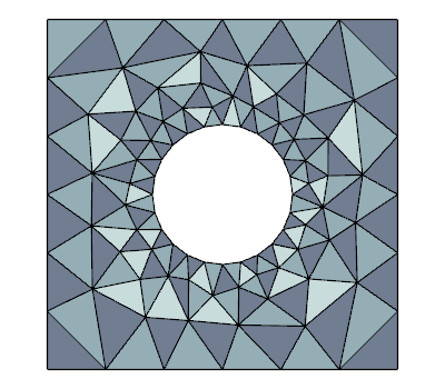
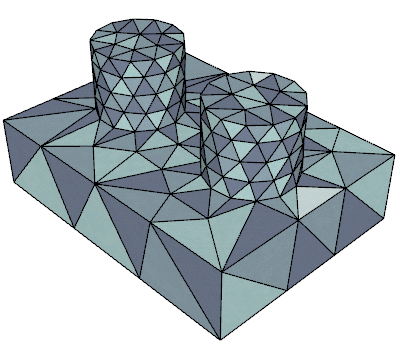
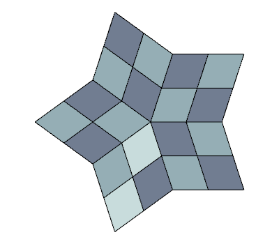
Fig. 1: Three unstructured meshes, using triangles, tetrahedra, and quadrilaterals.

Next we consider problems with different meshes, including unstructured triangular, quadrilateral, and tetrahedral meshes, using in particular the meshes shown in Figure 1 at various levels of refinement. The problem is the same as in Section 7.1 except for the mesh. We fix $p=1$ and focus on the scalability with respect to $h$. The convergence results in Table 4 demonstrate that the preconditioner continues to be scalable in these more general settings.

Table 4: Number of CG iterations and average reduction factors per iteration (in parenthesis) for several unstructured meshes at various refinement levels.

refine	triangles	tetrahedra	quadrilaterals
0	13 (0.34)	08 (0.17)	09 (0.21)
1	14 (0.37)	11 (0.27)	12 (0.31)
2	14 (0.36)	13 (0.35)	13 (0.32)
3	14 (0.35)	15 (0.39)	13 (0.33)
4	14 (0.36)	16 (0.42)	12 (0.31)
5	14 (0.37)		12 (0.30)
6	15 (0.38)		12 (0.30)
7	15 (0.38)		12 (0.29)
8	15 (0.39)		12 (0.30)

7.4 Behavior of solver with respect to contrast in coefficient

In the following numerical results the coefficient $\kappa$ in (1) is piecewise constant, chosen randomly on each element, so that it is 1 with probability 1/2 and $\kappa_{0}$ with probability 1/2, where $\kappa_{0}$ is a specified constant across the mesh. Here the ${\tt{B}}^{o}$ component in (25) is constructed from an $H^{1}$ matrix assembled from the bilinear form in (1) using the varying coefficient $\kappa$, and ${\tt{P}}^{f}$ is constructed as usual using the principal minor of ${\tt{A}}$, which also includes the coefficient $\kappa$. In Table 5 we report the number of iterations and average reduction factor for several refinement levels and choice of contrast $\kappa_{0}$. The results show that the problem gets harder for high-contrast coefficients, as expected, but the solver still performs well.

Table 5: Number of CG iterations and average reduction factors per iteration (in parenthesis) for various values of the contrasts coefficient $\kappa_{0}$.

	contrast
elements	1e-06	1e-04	1e-02	1e+00	1e+02	1e+04
64	13 (0.29)	12 (0.31)	10 (0.24)	5 (0.06)	8 (0.15)	12 (0.24)
512	31 (0.64)	29 (0.61)	14 (0.36)	7 (0.10)	11 (0.27)	17 (0.44)
4096	64 (0.80)	49 (0.75)	15 (0.39)	8 (0.16)	13 (0.33)	33 (0.64)
32768	119 (0.89)	73 (0.83)	16 (0.41)	9 (0.20)	14 (0.36)	43 (0.72)

8 Conclusions

In this paper we presented a scalable preconditioner for the primal DPG formulation of the Poisson problem based on parallel algebraic multigrid techniques. We proved that the preconditioner is optimal under certain assumptions on the mesh and problem coefficients. We also demonstrated that the new algorithm performs well on a wide variety of problems, including some where the theory is not applicable. Due to its algebraic nature, the preconditioner is easy to apply in practice, and has a freely available implementation in the MFEM library.

References

- [1] M. Ainsworth and L. Demkowicz, Explicit polynomial preserving trace liftings on a triangle, Math. Nachr., 282 (2009), pp. 640–658.
- [2] A. Baker, R. Falgout, T. Kolev, and U. Yang, Scaling hypre’s multigrid solvers to 100,000 cores, in High Performance Scientific Computing: Algorithms and Applications, Springer, 2012, pp. 261–279. LLNL-JRNL-479591.
- [3] A. T. Barker, S. C. Brenner, E.-H. Park, and L.-Y. Sung, A one-level additive Schwarz preconditioner for a discontinuous Petrov-Galerkin method, in Domain Decomposition Methods in Science and Engineering XXI, vol. 98 of Lecture Notes in Computational Science and Engineering, 2014, pp. 417–425.
- [4] C. Bernardi, Optimal finite-element interpolation on curved domains, SIAM J. Numer. Anal., 26 (1989), pp. 1212–1240.
- [5] D. Boffi, F. Brezzi, and M. Fortin, Mixed Finite Element Methods and Applications, vol. 44 of Springer Series in Computational Mathematics, Springer Berlin Heidelberg, 2013. doi: 10.1007/978-3-642-36519-5.
- [6] T. Bouma, J. Gopalakrishnan, and A. Harb, Convergence rates of the DPG method with reduced test space degree, Computers and Mathematics with Applications, 68 (2014), pp. 1550–1561.
- [7] T. A. Brunner and T. V. Kolev, Algebraic multigrid for linear systems obtained by explicit element reduction, SIAM J. Sci. Comput., 33 (2011), pp. 2706–2731.
- [8] V. M. Calo, N. O. Collier, and A. H. Niemi, Analysis of the discontinuous Petrov-Galerkin method with optimal test functions for the Reissner-Mindlin plate bending model, Computers and Mathematics with Applications, 66 (2014), pp. 2570–2586.
- [9] C. Carstensen, L. Demkowicz, and J. Gopalakrishnan, Breaking spaces and forms for the dpg method and applications including maxwell equations, Computers and Mathematics with Applications, 72 (2016), pp. 494–522.
- [10] J. Chan, N. Heuer, T. Bui-Thanh, and L. Demkowicz, A robust DPG method for convection-dominated diffusion problems II: adjoint boundary conditions and mesh-dependent test norms, Comput. Math. Appl., 67 (2014), pp. 771–795.
- [11] M. Costabel, M. Dauge, and L. Demkowicz, Polynomial extension operators for , and -spaces on a cube, Math. Comp., 77 (2008), pp. 1967–1999.
- [12] L. Demkowicz and J. Gopalakrishnan, A class of discontinuous Petrov–Galerkin methods. Part I: The transport equation, Comp. Meth. Appl. Math. Engrg., 199 (2010), pp. 1558–1572.
- [13] , A class of discontinuous Petrov–Galerkin methods. Part II: Optimal test functions, Num. Meth. Part. Diff. Eq., 27 (2011), pp. 70–105.
- [14] , A class of discontinuous Petrov–Galerkin methods. Part IV: The optimal test norm and time–harmonic wave propagation in 1D, J. Comp. Phys., 230 (2011), pp. 2406–2432.
- [15] L. Demkowicz and J. Gopalakrishnan, A primal DPG method without a first-order reformulation, Comp. Math. Applic., 66 (2013), pp. 1058–1064.
- [16] L. Demkowicz and J. Gopalakrishnan, Discontinuous Petrov Galerkin (DPG) method, in Encyclopedia of Computational Mechanics, Wiley Computational Mechanics Online, 2016 (to appear).
- [17] L. Demkowicz, J. Gopalakrishnan, and A. H. Niemi, A class of discontinuous Petrov–Galerkin methods. Part III: Adaptivity, Appl. Numer. Math., (2011), p. in press.
- [18] L. Demkowicz, J. Gopalakrishnan, and J. Schöberl, Polynomial extension operators. Part III., Math. Comp., 81 (2012), pp. 1289–1326.
- [19] J. Gopalakrishnan and W. Qiu, An analysis of the practical DPG method, Mathematics of Computation, 83 (2014), pp. 537–552.
- [20] J. Gopalakrishnan and J. Schöberl, Degree and wavenumber [in]dependence of Schwarz preconditioner for the DPG method, in Spectral and High Order Methods for Partial Differential Equations (ICOSAHOM 2014), R. M. Kirby, M. Berzins, and J. S.Hesthaven, eds., no. 106 in Lecture Notes in Computational Science and Engineering, Springer, 2015, pp. 257–265.
- [21] V. E. Henson and U. M. Yang, BoomerAMG: A parallel algebraic multigrid solver and preconditioner, Appl. Numer. Math., 41 (2002), pp. 155–177.
- [22] R. Hiptmair and J. Xu, Nodal auxiliary space preconditioning in and spaces, SIAM J. Numer. Anal., 45 (2007), pp. 2483–2509 (electronic).
- [23] T. V. Kolev and P. S. Vassilevski, Parallel auxiliary space AMG solver for H(curl) problems, J. Comput. Math., 27 (2009), pp. 604–623.
- [24] , Parallel auxiliary space AMG solver for H(div) problems, SIAM J. Sci. Comput., 34 (2012), pp. A3079–A3098.
- [25] X. Li and X. Xu, Domain decomposition preconditioners for the discontinuous Petrov-Galerkin method, ESAIM: Mathematical Modelling and Numerical Analysis, in press (2016).
- [26] MFEM: Modular finite element methods. http://mfem.org.
- [27] S. Nepomnyaschikh, Domain decomposition methods, in Lectures on advanced computational methods in mechanics, vol. 1 of Radon Ser. Comput. Appl. Math., Walter de Gruyter, Berlin, 2007, pp. 89–159.
- [28] N. V. Roberts and J. Chan, A geometric multigrid preconditioning strategy for DPG system matrices, ArXiV Preprint: 1608.02567, (2016).