Learning with Hierarchical Gaussian Kernels

Abstract

We investigate iterated compositions of weighted sums of Gaussian kernels and provide an interpretation of the construction that shows some similarities with the architectures of deep neural networks. On the theoretical side, we show that these kernels are universal and that SVMs using these kernels are universally consistent. We further describe a parameter optimization method for the kernel parameters and empirically compare this method to SVMs, random forests, a multiple kernel learning approach, and to some deep neural networks.

1 Introduction

Although kernel methods such as support vector machines are one of the state-of-the-art methods when it comes to fully automated learning, see e.g. the recent independent comparison [7], the recent years have shown that on complex datasets such as image, speech and video data, they clearly fall short compared to deep neural networks.

One possible explanation for this superior behavior is certainly their deep architecture that makes it possible to represent highly complex functions with relatively few parameters. In particular, it is possible to amplify or suppress certain dimensions or features of the input data, or to combine features to new, more abstract features. Compared to this, standard kernels such as the popular Gaussian kernels simply treat every feature equally. In addition, most users of kernel machines probably stick to the very few standard kernels, often simply because there is in most cases no principled way for finding problem specific kernels. In contrast to this, deep neural networks offer yet another order of freedom to the user by making it easy to choose among many different architectures and other design decisions. This discussion shows that the class of deep neural networks offers potentially much more functions that may fit well to the problem at hand than classical kernel methods do. Therefore, if the training algorithms are able to find these good hypotheses while simultaneously controlling the inherent danger of overfitting (and the user picked a good design), then the recent success of deep networks does not seem to be so surprising after all. In particular, this may be an explanation for the types of data mentioned above, for which an equal and un-preprocessed use of all features may really not be the best idea, but for which there is also some biological insight suggesting certain building blocks of neural architectures. Moreover, the recent success of deep networks indicates that these ‘ifs’ can nowadays much better be controlled than 20 to 30 years ago. This naturally raises the question, whether and how certain aspects of deep neural networks can be translated into the kernel world without sacrificing the benefits of kernel-based learning, namely less ‘knobs’ an unexperienced user can play with, the danger of getting stuck in poor local minima, a more principled statistical understanding, and last but not least, their success in situations in which no human expert is in the loop.

Of course, the limitations of using simple single kernels have already been recognized before. Probably the first attempts in this direction are multiple kernel learning algorithms, see e.g. [12], which, in a nutshell, replace a single kernel by a weighted sum of kernels. The advantage of this approach is that finding these weights can again be formulated as a convex objective, while the disadvantage is the limited gain in expressive power unless the used dictionary of kernels is really huge. A more recent approach for increasing the expressive power is to construct complex kernels from simple ones by composing their feature maps in some form. Probably the first result in this direction can be found in [3], in which the authors described the general setup and considered some particular constructions. Moreover, this idea was adopted in [15], where the authors considered sums of kernels in each composition step and established bounds on the Rademacher chaos complexities. Similarly, [18] considered such sums in the decomposition step, but they mostly restricted their considerations to a single decomposition step, for which they established a generalization bound based on the pseudo-dimension. Furthermore, [17] investigated compositions, in which the initial map is not a kernel feature map, but the map induced by a deep network. All these articles also present some experimental results indicating the benefits of the more expressive kernels. Similarly, [16] reports some experiments with a linear SVM as the top layer of a deep network. Another approach can be found in [9], where the authors construct hierarchical convolutional kernels for image data, and finally [1] proposed a multiple kernel learning approach, which is also called hierarchical kernels. However, besides the name, that paper has little similarity to our approach.

In this paper we adopt the idea of iteratively composing weighted sums of kernels in each layer. Unlike the papers mentioned above, however, we focus on sums of Gaussian kernels composed with Gaussian kernels. Besides an illustrative interpretation of the construction, which highlights the similarities to deep architectures, we show that the resulting kernels are universal and that the corresponding SVMs become universally consistent. To the best of our knowledge our paper is thus the first that does not only investigate some statistical properties of iterated kernels, but also considers their approximation properties. We further describe a possible kernel parameter optimization algorithm in detail, and last but not least we report results from extensive experiments comparing our algorithm against SVMs, random forests, the hierarchical kernel learning (HKL) of [1] and deep neural networks. Here it turns out that even for rather small compositions our approach consistently outperforms SVMs and HKL. Moreover, our experiments indicate an advantage over deep neural networks for which the architecture is automatically determined by cross validation and they further show that our approach performs better than random forests.

The rest of this paper is organized as follows: In Section 2 we introduce our class of kernels and in Section 3 we present their theoretical analysis. Section 4 contains the description of the parameter optimization, and the experiments are reported in Section 5. The proofs and some auxiliary theorems can be found in the appendix.

2 Hierarchical Gaussian Kernels

In this section we introduce the central object of this paper, namely hierarchical Gaussian kernels. Let us begin by recalling some basic facts on kernels from [14, Chapter 4]. To this end, let $k:X\times X\to\mathbb{R}$ be a function. Then $k$ is a kernel, if there exists a Hilbert space $H$ and a map $\Phi_{0}:X\to H_{0}$ such that

$$k(x,x^{\prime})=\langle\Phi_{0}(x),\Phi_{0}(x^{\prime})\rangle\,,\qquad\qquad x,x^{\prime}\in X.$$

In this case, $\Phi_{0}$ and $H_{0}$ are said to be a feature map and a feature space of $k$, respectively. It is well known, that every such kernel possesses a unique reproducing kernel Hilbert space (RKHS) $H$ and this RKHS is a feature space of $k$ with respect to the canonical feature map $\Phi:X\to H$ given by $\Phi(x):=k(x,\cdot)$, $x\in X$. Moreover, by definition $H$ consists of functions $h:X\to\mathbb{R}$, and if $k$ is continuous, so are the functions in $H$. Let us now assume that $X$ is a compact metric space and that $k$ is a continuous kernel. Then $k$ is said to be universal, if its RKHS $H$ is dense in the space $C(X)$ of continuous functions $f:X\to\mathbb{R}$ with respect to the supremums norm $\|\cdot\|_{\infty}$. Furthermore, we say that $k$ is injective, if its canonical feature map is injective. Recall that universal kernels are injective, see e.g. [14, Lemma 4.55]. Moreover, the injectivity is actually shared by all feature maps of $k$, see Lemma A.1 for details. In particular, it is easy to see that besides universal kernels many other kernels are injective, too. For example, the linear kernel $k(x,x^{\prime}):=\langle x,x^{\prime}\rangle$ on $\mathbb{R}^{d}$ is injective since one of its feature maps is the identity on $\mathbb{R}^{d}$, which, of course, is injective. Finally, note that if $k$ is injective on $X$ then its restriction $k_{|X^{\prime}\times X^{\prime}}$ onto some subset $X^{\prime}\subset X$ is still injective.

Probably one of the best known universal kernel on $X\subset\mathbb{R}^{d}$ is the standard Gaussian RBF kernel $k_{\gamma}$ with width $\gamma>0$, which is given by

$$k_{\gamma,X}(x,x^{\prime}):=\exp\bigl{(}-\gamma^{-2}\|x-x^{\prime}\|_{2}^{2}\bigr{)}\,,\qquad\quad x,x^{\prime}\in X\,,$$

where $\|\cdot\|_{2}$ denotes the standard Euclidean norm on $\mathbb{R}^{d}$. In the following we denote its RKHS by $H_{\gamma,X}$. Now, it is well-known that this construction can actually be extended to subsets $Z$ of more general Hilbert spaces $H$, that is,

$$k_{\gamma,Z}(z,z^{\prime}):=\exp\bigl{(}-\gamma^{-2}\|z-z^{\prime}\|_{H}^{2}\bigr{)}\,,\quad z,z^{\prime}\in Z.$$ (1)

is again a kernel, whose RKHS will be denoted by $H_{\gamma,Z}$. In particular, if we have a map $\Phi:X\to H$, then

$$k_{\gamma,X,H}(x,x^{\prime}):=\exp\bigl{(}-\gamma^{-2}\|\Phi(x)-\Phi(x^{\prime})\|_{H}^{2}\bigr{)}$$ (2)

defines a new kernel on $X$, see e.g. [14, Lemma 4.3], and if $\Phi_{\gamma,Z}:Z\to H_{\gamma,Z}$ denotes the canonical feature map of $k_{\gamma,Z}$, then $\Phi_{\gamma,Z}\circ\Phi:X\to H_{\gamma,Z}$ is a feature map of $k_{\gamma,X,H}$. Now, note that these assumptions on $\Phi$ and $H$ are equivalent to saying that $H$ is a feature space of the kernel given by $k(x,x^{\prime})=\langle\Phi(x),\Phi(x^{\prime})\rangle$, and since we have $\|\Phi(x)-\Phi(x^{\prime})\|_{H}^{2}=k(x,x)-2k(x,x^{\prime})+k(x^{\prime},x^{\prime})$, we can also express (2) by the kernel $k$. In the following, we call kernels $k_{\gamma,X,H}$ of the form above hierarchical Gaussian kernels. For later use we note that these kernels are universal if $X$ is a compact metric space and $\Phi$ is continuous and injective, see Theorem A.2 for details.

Our next goal is to investigate hierarchical Gaussian kernels (2) for which $H$ and its kernel $k$ is of rather complicated form. To this end, we write, for $x=(x_{1},\dots,x_{m})\in\mathbb{R}^{m}$ and $I\subset\{1,\dots,m\}$,

$$x_{I}:=(x_{i})_{i\in I}$$

for the vector projected onto the coordinates listed in $I$. Note that if $X$ is compact then the image $X_{I}$ of this projection is also compact since continuous images of compact sets are compact. Let us now assume that we have non-empty sets $I_{1},\dots,I_{l}\subset\{1,\dots,m\}$ and $X\subset\mathbb{R}^{m}$, some weights $w_{1},\dots,w_{l}>0$, as well kernels $k_{i}$ on $X_{I_{i}}$ for all $i=1,\dots,l$. For $I:=I_{1}\cup\cdots\cup I_{l}$, we then define a new kernel on $X_{I}$ by

$$k(x,x^{\prime}):=\sum_{i=1}^{l}w_{i}^{2}k_{i}\bigl{(}x_{I_{i}},x^{\prime}_{I_{i}}\bigr{)}\,,\qquad x,x^{\prime}\in X_{I}.$$ (3)

One can show, that hierarchical Gaussian kernels of the form (3) can be computed by a simple product formula, see Lemma A.3. The following definition considers iterations of (3).

Definition 2.1.

Let $k$ be a kernel of the form (3) and $H$ be its RKHS. Then the resulting hierarchical Gaussian kernel $k_{\gamma,X_{I},H}$ is said to be of depth

1. $m=1$, if all kernels $k_{1},\dots,k_{l}$ in (3) are linear.

2. $m>1$, if all $k_{1},\dots,k_{l}$ in (3) are hierarchical Gaussian kernels of depth $m-1$.

To illustrate the definition above, we note that hierarchical kernels of depth 1 are of the form

$$k_{\mathbf{v}}(x,x^{\prime}):=\exp\bigl{(}-\sum_{i\in I}v_{i}^{2}(x_{i}-x_{i}^{\prime})^{2}\bigr{)},\quad x,x^{\prime}\in X,$$ (4)

for some suitable $\mathbf{v}:=(v_{i})_{i\in I}$ with $v_{i}>0$ for all $i\in I$. In other words, they only differ from standard Gaussian kernels on $X_{I}$ by their inhomogeneous width parameter $\mathbf{v}$. For this reason we sometimes also call kernels of the form (4) inhomogeneous Gaussian kernels.

To derive an explicit formula for depth-2-kernels, we fix some $I_{1},\dots,I_{l}\subset\{1,\dots,d\}$, some first layer weight vectors $\mathbf{v}_{1}=(v_{i,1})_{i\in I_{1}},\dots,\mathbf{v}_{l}=(v_{i,l})_{i\in I_{l}}$ and a second layer weight vector $\mathbf{w}=(w_{1},\dots w_{l})$. Writing $\mathbf{W}^{(1)}:=(\mathbf{v}_{1},\dots\mathbf{v}_{l})$, the hierarchical Gaussian kernel $k_{\mathbf{W}^{(1)},\mathbf{w},\gamma}$ of depth 2 that is build upon the kernels $k_{\mathbf{v}_{1}},\dots k_{\mathbf{v}_{l}}$ and weights $\mathbf{w}=(w_{1},\dots w_{l})$ is given by

$$k_{\mathbf{W}^{(1)},\mathbf{w},\gamma}(x,x^{\prime})$$ (5)

$$=\exp\biggl{(}-2\gamma^{-2}\sum_{i=1}^{l}w_{i}^{2}\bigl{(}1-k_{\mathbf{v}_{i}}(x_{I_{i}},x^{\prime}_{I_{i}})\bigr{)}\biggr{)}$$

$$=\exp\Biggl{(}-2\gamma^{-2}\sum_{i=1}^{l}w_{i}^{2}\biggl{(}1-\exp\Bigl{(}-\sum_{j\in I_{i}}v_{j,i}^{2}(x_{j}-x_{j}^{\prime})^{2}\Bigr{)}\biggr{)}\Biggr{)}\,.$$

Here we note that we used the fact that all first layer kernels $k_{\mathbf{v}_{1}},\dots,k_{\mathbf{v}_{l}}$ are normalized, that is $k_{\mathbf{v}_{i}}(x,x)=1$ for all $x\in X_{I_{i}}$. Also note that the parameter $\gamma$ in (5) can be consumed by the weights $\mathbf{w}$. In the following, we therefore use the shorthand $k_{\mathbf{W}^{(1)},\mathbf{w}}:=k_{\mathbf{W}^{(1)},\mathbf{w},1}$. Finally, if $k_{\mathbf{W}^{(1)}_{1},\mathbf{w}_{1}^{(2)}},\dots,k_{\mathbf{W}^{(1)}_{l},\mathbf{w}_{l}^{(2)}}$ are some hierarchical kernels of depth 2, and $\mathbf{w}=(w_{1},\dots w_{l})$ is a third layer weight vector, then the corresponding kernel $k$ of depth 3 is given by

$$k_{\mathbf{W}^{(1)},\mathbf{W}^{(2)},\mathbf{w},\gamma}(x,x^{\prime})$$ (6)

$$=\exp\biggl{(}-2\gamma^{-2}\sum_{i=1}^{l}w_{i}^{2}\bigl{(}1-k_{\mathbf{W}^{(1)}_{i},\mathbf{w}_{i}^{(2)}}(x_{I_{i}},x^{\prime}_{I_{i}})\bigr{)}\biggr{)}\,,$$

where we used the notation $\mathbf{W}^{(1)}:=(\mathbf{W}^{(1)}_{1},\dots\mathbf{W}^{(1)}_{l})$ and $\mathbf{W}^{(2)}:=(\mathbf{w}_{1}^{(2)},\dots\mathbf{w}_{l}^{(2)})$. Repeating these calculations, we see that hierarchical kernels of depth $m$ are given by

$$k_{\mathbf{W}^{(1)},\dots,\mathbf{W}^{(m-1)},\mathbf{w},\gamma}(x,x^{\prime})$$ (7)

$$=\exp\biggl{(}-2\gamma^{-2}\sum_{i=1}^{l}w_{i}^{2}\bigl{(}1-k_{\mathbf{W}^{(1)}_{i},\dots,\mathbf{W}^{(m-2)}_{i},\mathbf{w}_{i}^{(m-1)}}(x_{I_{i}},x^{\prime}_{I_{i}})\bigr{)}\biggr{)}\,,$$

where $k_{\mathbf{W}^{(1)}_{i},\dots,\mathbf{W}^{(m-2)}_{i},\mathbf{w}_{i}^{(m-1)}}$ denote hierarchical kernels of depth $m-1$ with $\gamma=1$. Note that because of the recursive definition of hierarchical kernels, the number of children kernels $l$ may differ in each parent kernel. To be more precise, the kernels $k_{\mathbf{W}^{(1)}_{i},\dots,\mathbf{W}^{(m-2)}_{i},\mathbf{w}_{i}^{(m-1)}}$ in (7) are build by $l_{i}$ many kernels of depth $m-2$, and in general we have both $l_{i}\neq l_{j}$ and $l_{i}\neq l$.

Figure 1: Illustration of a possible hierarchical Gaussian kernel of depth 3.

3 Mathematical Analysis

In this section we analyze hierarchical Gaussian kernels theoretically. Our main result shows that these kernels are universal under a simple and natural assumption. Based on this, we then show that SVMs using such kernels are universally consistent.

Theorem 3.1.

Let $X\subset\mathbb{R}^{d}$ be compact. Then every hierarchical Gaussian kernel $k_{\gamma,X_{I},H}$ of some depth is universal if $I=\{1,\dots,d\}$.

Proof of Theorem 3.1: Let us first consider the case $I=\{1,\dots,d\}$. If $k_{\gamma,X_{I},H}$ has depth 1, then the assertion follows by Theorem A.4 and the fact that linear kernels are injective. Moreover, for higher depths the universality follows from Theorem A.4 and the injectivity of universal kernels. ∎

Let us fix some $Y\subset\mathbb{R}$. In the following, a measurable function $L:Y\times\mathbb{R}\to[0,\infty)$ is called a loss. We further say that the loss $L$ is convex or continuous, if it is convex or continuous with respect to its second argument. Moreover, $L$ is called Lipschitz continuous, if

$$|L|_{1}:=\sup_{y,t\neq t^{\prime}}\frac{\bigl{|}L(y,t)-L(y,t^{\prime})\bigr{|}}{|t-t^{\prime}|}<\infty\,,$$

where the supremum is taken over all possible values of $y,t$, and $t^{\prime}$. Finally, we say that $L$ can be clipped at some $M>0$ if $L(y,{{}^{\textstyle\smallfrown}}t\hskip 2.15277pt)\,\leq\,L(y,t)$, where ${{}^{\textstyle\smallfrown}}t\hskip 2.15277pt$ denotes the clipped value of $t$ at $\pm M$, that is ${{}^{\textstyle\smallfrown}}t\hskip 2.15277pt:=\max\{-M,\min\{M,t\}\}$. Recall that [14, Lemma 2.23] gives a simple characterization of convex, clippable losses. In particular, the hinge loss is clippable, and so are the least squares loss and the pinball loss, if $Y$ is bounded. Furthermore, all these losses are convex and continuous, and the hinge loss and the pinball loss are also Lipschitz continuous. Given a distribution $P$ on $X\times Y$ and a (measurable) function $f:X\to\mathbb{R}$, the $L$-risk of $f$ is

$${{\cal R}_{L,P}(f)}:=\int_{X\times Y}L(y,f(x))\,dP(x,y)\,.$$

Moreover, the Bayes risk ${{\cal R}_{L,P}^{*}}:=\inf\{{{\cal R}_{L,P}(f)}|f:X\to\mathbb{R}\}$ is the smallest possible risk. Finally, the empirical risk with respect to some data set $D=((x_{1},y_{1}),\dots,(x_{n},y_{n}))$ is, as usual,

$${{\cal R}_{L,D}(f)}:=\frac{1}{n}\sum_{i=1}^{n}L\bigl{(}y_{i},f(x_{i})\bigr{)}\,.$$

Now let $L$ be a convex loss, $H$ be an RKHS over $X$ and $\lambda>0$ be some regularization parameter. Then the SVM decision function for the data set $D$ is the unique solution of the optimization problem

$$f_{D,\lambda}=\arg\min_{f\in H}\lambda\|f\|_{H}^{2}+{{\cal R}_{L,D}(f)}\,.$$ (8)

The statistical properties of these learning methods have been extensively studied in the last 15 years, so that a rich theory is now available, see e.g. [5, 14]. One key concept of this theory is the so-called approximation error function

$$A(\lambda):=\inf_{f\in H}\lambda\|f\|_{H}^{2}+{{\cal R}_{L,P}(f)}-{{\cal R}_{L,P}^{*}}\,,\qquad\lambda>0\,,$$

which roughly speaking describes the regularization error in an infinite-sample regime. In particular, we have $\lim_{\lambda\to 0}A(\lambda)=0$ if $X$ is compact, $Y$ is bounded, $H$ is universal, and $L$ is one of the losses mentioned above. We refer to [14, Lemma 5.15 and Corollary 5.29] for the derivation of these results and to [14, Chapter 5.5] for further results in the case of unbounded $Y$.

With the help of these definitions we can now present the following oracle inequality, which is a direct derivation from [14, Theorem 7.22] and the fact that universal kernels have a separable RKHS.

Theorem 3.2.

Let $X\subset\mathbb{R}^{d}$ be compact, $I=\{1,\dots,d\}$, and $k_{\gamma,X_{I},H}$ be a hierarchical Gaussian kernel of some depth. Moreover, let $L$ be a Lipschitz continuous loss that can be clipped at some $M>0$ and that satisfies

$$L(y,t)\leq B\,,$$

for some $B>0$ and all $y\in Y$, $t\in[-M,M]$. Then there exists a constant $K>0$ such that for all fixed $\tau\geq 1$, $n\geq 2$, and $\lambda>0$ the SVM associated with $L$ and $k_{\gamma,X_{I},H}$ satisfies

$${{\cal R}_{L,P}({{}^{{}^{\textstyle\smallfrown}}}f_{D,\lambda})}-{{\cal R}_{L,P}^{*}}$$

$$\quad\leq 9A(\lambda)+K\frac{\ln n}{\lambda n}+\frac{15\tau}{n}\sqrt{\frac{A(\lambda)}{\lambda}}+\frac{300B\tau}{\sqrt{n}}$$

with probability $P^{n}$ not less than $1-3e^{-\tau}$. In particular, the SVM is universally consistent if we pick a regularization sequence $(\lambda_{n})$ with $\lambda_{n}\to 0$ and $\frac{\ln n}{\lambda_{n}n}\to 0$, that is

$${{\cal R}_{L,P}({{}^{{}^{\textstyle\smallfrown}}}f_{D,\lambda_{n}})}\to{{\cal R}_{L,P}^{*}}$$

in probability for all distributions $P$ on $X\times Y$.

Note that the oracle inequality above can also be used to derive learning rates, if, as usual, an assumption on the behavior of $A(\,\cdot\,)$ is imposed. However, translating such a behavior into an assumption on $P$ is even for standard Gaussian kernels a highly non-trivial task, see e.g. [14, Chapter 8.2] and [6], since by [11] all reasonable results in this direction require the kernel parameter $\gamma$ to change with $n$, too. While for inhomogeneous kernels there is still some hope to adapt the analysis of [6], the situation becomes extraordinarily more difficult for deeper Gaussian kernels. In addition, even considering inhomogeneous kernels only, would most likely be more complicated and lengthy than the already involved analysis of [6], and hence this task is clearly out of the scope of this paper. Similarly, our statistical analysis can be sharpened if we add an assumption on the entropy number or eigenvalue behavior, see e.g. [14, Theorem 7.23 and Chapter 7.5] but a refined analysis in this direction is, for essentially the same reasons as above, again out of the scope of this paper. Finally, note that some assumptions made in Theorem 3.2 are not necessary for deriving consistency. For example, the Lipschitz continuity, the bound in terms of $B$, and the clipping assumption can be removed for the price of a looser oracle inequality. For examples in this direction we refer to [14, Chapters 6.4, 7.4, and 9.2].

4 Parameter Optimization

For the standard Gaussian kernels it is well-known both empirically and theoretically that the learning performance of the resulting SVM heavily depends on the chosen width parameter $\gamma$. Clearly, we can expect a similar dependence on the weight parameters ${\mathbf{W}}$ for hierarchical Gaussian kernels, but for these parameters, finding good values is a potentially more difficult problem. In this section we address this issue by presenting an optimization strategy, which in the next section is empirically validated.

In the following let $D=((x_{1},y_{1}),\dots,(x_{n},y_{n}))$ and $D^{\prime}=((x^{\prime}_{1},y^{\prime}_{1}),\dots,(x^{\prime}_{n^{\prime}},y^{\prime}_{n^{\prime}}))$ be two data sets. Let us assume that $D$ is used for training, that is, $D$ is used to find an SVM decision function

$$f_{D,\lambda,\mathbf{W},\gamma}=\sum_{i=1}^{n}\alpha_{i}k_{\mathbf{W},\gamma}(x_{i},\,\cdot\,)\,,$$ (9)

where $\mathbf{W}$ denotes the collection of weights of a hierarchical Gaussian kernel of fixed architecture. Let us further assume that $D^{\prime}$ is used to validate the quality of the weights $\mathbf{W}$, that is, the empirical risk

$${{\cal R}_{L,D^{\prime}}(f_{D,\lambda,\mathbf{W},\gamma})}=\frac{1}{n^{\prime}}\sum_{j=1}^{n^{\prime}}L\bigl{(}y_{j}^{\prime},f_{D,\lambda,\mathbf{W},\gamma}(x_{j}^{\prime})\bigr{)}$$ (10)

is computed. Clearly, by minimizing this validation risk, we may hope to find a suitable collection of weights $\mathbf{W}$. Note however, that if we change the weights $\mathbf{W}$ of the kernel $k_{\mathbf{W},\gamma}$ to decrease the validation risk (10), then the right-hand side of (9) is no longer the SVM solution with respect to the new kernel $k_{\mathbf{W},\gamma}$. Therefore, a recomputation of $\alpha:=(\alpha_{1},\dots\alpha_{n})$ becomes necessary, and the same may be true for the hyper-parameters $\lambda$ and $\gamma$. The overall objective is therefore threefold: a) for fixed $\lambda,\gamma,\alpha$ we wish to minimize

$${{\cal R}}_{L,D^{\prime}}(\lambda,\gamma,\alpha,\mathbf{W})$$ (11)

$$\qquad:=\frac{1}{n^{\prime}}\sum_{j=1}^{n^{\prime}}L\biggl{(}y_{j}^{\prime},\sum_{i=1}^{n}\alpha_{i}k_{\mathbf{W},\gamma}(x_{i},x_{j}^{\prime})\biggr{)}$$

with respect to $\mathbf{W}$; b) we need to determine $\alpha$ for fixed $\lambda$, $\gamma$, and $\mathbf{W}$ by solving the SVM optimization problem (8); and c) we need to update the hyper-parameters $\lambda$ and $\gamma$. Clearly, b) is nowadays standard, and for c) the most widely adopted approach is grid search based on cross validation. Unfortunately, however, there is no hope that the objective function (11) is convex in $\mathbf{W}$, so that minimizing it is a challenge. In addition, brute-force methods such as grid search over all combinations of weights are far too expensive. However, finding the ‘right’ weights for learning may be a smaller problem compared to, e.g., neural networks, since even for non-optimal weights the corresponding SVM is consistent if we split the learning process into two independent phases in which we first look for weights on one (small) chunk of the data and then retrain an SVM with these weights on another (larger) chunk of the data, see Theorem 3.2. In this sense, our task therefore reduces to finding ’good’ weights that promise to expedite the learning process.

To find such good weights, we will now present a combination of a local minimizer, namely gradient descent, and a global minimization heuristic, namely simulated annealing, but certainly, other approaches such as stochastic gradient descent and its modifications, which are popular for training deep neural networks, may be serious alternatives that should be investigated in the future. In addition, one could, at least in principle, combine the three objectives a)-c) into one by a simple summation. However, this would change the SVM objective function so that we loose both the well-founded statistical theory for SVMs and the ability to use off-the-shelf solvers for (8). For this reason, we decided to ignore this possibility. The goal of the remainder of this section is to describe the two optimization strategies for $\mathbf{W}$ and how they were combined with the steps b) and c).

Let us begin by describing some details of gradient descent for (11). To this end, let $w$ be a weight contained in $\mathbf{W}$. If the loss $L$ is differentiable in its second argument, then a simple application of the chain rule shows that the partial derivative of (11) with respect to $w$ is given by

$$\frac{\partial}{\partial w}{{\cal R}}_{L,D^{\prime}}(\lambda,\gamma,\alpha,\mathbf{W})$$

$$=\frac{1}{n^{\prime}}\sum_{j=1}^{n^{\prime}}L^{\prime}\biggl{(}y_{j}^{\prime},\sum_{i=1}^{n}\alpha_{i}k_{\mathbf{W},\gamma}(x_{i},x_{j}^{\prime})\biggr{)}\sum_{i=1}^{n}\alpha_{i}\frac{\partial}{\partial w}k_{\mathbf{W},\gamma}(x_{i},x_{j}^{\prime})\,,$$

where $L^{\prime}$ denotes the derivative of $L$ in its second argument. To implement gradient descent we consequently need to know the partial derivatives $\frac{\partial}{\partial w}k_{\mathbf{W},\gamma}$, which are recursively computed in the following lemma for which the proof and an example can be found in the appendix.

Lemma 4.1.

Let $k_{\mathbf{W}^{(1)},\dots,\mathbf{W}^{(m-1)},\mathbf{w},\gamma}$ be a hierarchical Gaussian kernel of depth $m$ of the form (7) and $H$ be its RKHS. Then the parameter derivatives of the highest layer can be computed by

$$\frac{\partial}{\partial w_{j}}k_{\mathbf{W}^{(1)},\dots,\mathbf{W}^{(m-1)},\mathbf{w},\gamma}$$

$$\qquad=-4\gamma^{-2}w_{j}\bigl{(}1-k_{\mathbf{W}^{(1)}_{j},\dots,\mathbf{W}^{(m-2)}_{j},\mathbf{w}_{j}^{(m-1)}}\bigr{)}$$

$$\qquad\quad\cdot k_{\mathbf{W}^{(1)},\dots,\mathbf{W}^{(m-1)},\mathbf{w},\gamma}\,.$$

Moreover, the parameter derivative of a weight $w$ occurring in a lower layer of the $j$-th node can be computed by recursively using the formula

$$\frac{\partial}{\partial w}k_{\mathbf{W}^{(1)},\dots,\mathbf{W}^{(m-1)},\mathbf{w},\gamma}$$

$$\qquad=2\gamma^{-2}w_{j}^{2}\frac{\partial}{\partial w}k_{\mathbf{W}^{(1)}_{j},\dots,\mathbf{W}^{(m-2)}_{j},\mathbf{w}_{j}^{(m-1)}}\,.$$

With the help of the formulas for the partial derivatives the gradient descent step at iteration $i$ now becomes

$$\mathbf{W}_{i+1}=\mathbf{W}_{i}-\eta\nabla{{\cal R}_{L,D^{\prime}}(\lambda,\gamma,\alpha,\mathbf{W}_{i})}\,,$$

where the gradient $\nabla{{\cal R}_{L,D^{\prime}}(\lambda,\gamma,\alpha,\mathbf{W}_{i})}$ is the vector of partial derivatives and $\eta$ is the step size. Although the step size is often simply a function of $i$, we decided to be more conservative, namely, we determined $\eta$ by a line search based on the Armijo–Goldstein condition, see e.g. [2, Chapter 3.5]. This choice ensures that we will find a local minimum, but on the other hand, it certainly hinders a wider inspection of the parameter space. Like for neural networks less conservative approaches may thus turn out to be more efficient in the future.

In this paper we decided to address the danger of getting stuck in a poor local minimum of the non-convex objective function (11) by simulated annealing, see [10, Chapter 10.12]. In iteration $i$ of our adaptation of this meta-heuristic we randomly picked one weight $w$ from the current weights $\mathbf{W}_{i}$, changed it randomly to obtain $\mathbf{W}_{i+1}$, and then kept the change if either an improvement of the objective function (11) was obtained, that is $\Delta:={{\cal R}_{L,D^{\prime}}(\lambda,\gamma,\alpha,\mathbf{W}_{i+1})}-{{\cal R}_{L,D^{\prime}}(\lambda,\gamma,\alpha,\mathbf{W}_{i})}<0$, or a uniformly generated random number $r_{i+1}\in[0,1]$ satisfied

$$r_{i+1}<0.5\exp\Bigl{(}-\frac{100i}{\sqrt{N}}\cdot\frac{\Delta}{{{\cal R}_{L,D^{\prime}}(\lambda,\gamma,\alpha,\mathbf{W}_{i})}}\Bigr{)}\,.$$

Here $N$ denotes the total number of iterations.

Algorithm 1 Optimization of weights

0:  A dataset $D$, a hierarchical Gaussian kernel $k_{\mathbf{W}}$ of some depth, $L,M,N_{1},N_{2},N_{3}\geq 1$.

0:  Some good values for the weights contained in $\mathbf{W}$.

1:  Split the data set $D$ into three random parts $D_{1}$, $D_{2}$, and $D_{3}$.

2:  for all $i=1,\dots,M$ do

3:     Train an SVM $f_{D_{1},\lambda,\mathbf{W}}$ of the form (9) with $k_{\mathbf{W},\gamma}$ on $D_{1}$ including grid search for $\lambda$ and $\gamma$.

4:     Optimize ${{\cal R}_{L,D_{2}}(\lambda,\gamma,\alpha,\mathbf{W})}$ with respect to $\mathbf{W}$ by simulated annealing with $N_{1}$ steps.

5:     for all $j=1,\dots,L$ do

6:        if Achieved local minimum of ${{\cal R}_{L,D_{2}}(\lambda,\gamma,\alpha,\mathbf{W})}$ in previous iteration then

7:           Optimize ${{\cal R}_{L,D_{2}}(\lambda,\gamma,\alpha,\mathbf{W})}$ with respect to $\mathbf{W}$ by simulated annealing with $N_{2}$ steps

8:        else

9:           Optimize ${{\cal R}_{L,D_{2}}(\lambda,\gamma,\alpha,\mathbf{W})}$ with respect to $\mathbf{W}$ by gradient descent with $N_{3}$ steps.

10:        end if

11:        Compute the test error ${{\cal R}_{L,D_{3}}(\lambda,\gamma,\alpha,\mathbf{W})}$ and store $\mathbf{W}$ if this error is smaller than the previous one.

12:     end for

13:     if Test error did not decrease in the loop above then

14:        Reshuffle $D_{1},D_{2}$ by splitting $D_{1}\cup D_{2}$ into two new parts $D_{1}$ and $D_{2}$.

15:     end if

16:  end for

17:  return weights $\mathbf{W}$ that achieved the smallest test error.

In the design of the overall optimization algorithm we again followed a very conservative approach, which focuses on reducing the risk of overfitting. Namely, we split the data set into three parts, from which the first two parts were used to find the SVM decision functions and the objective function (11). The third part was solely used to track a test error for $\mathbf{W}$. The final weight $\mathbf{W}$ was then chosen according to the minimal test error. The corresponding algorithm can be found in Algorithm 1.

5 Experiments

Data Set	SVM	HKL	Ours	RF	DNN
​​bank	​​.29780 $\pm$ .00240	​​.29387 $\pm$ .00283	​​.25959 $\pm$ .00388	​​.26868 $\pm$ .00269	​​.29310 $\pm$ .00247
​​cadata	​​.05382 $\pm$ .00156	​​.06247 $\pm$ .00138	​​.05252 $\pm$ .00186	​​.05087 $\pm$ .00153	​​.05500 $\pm$ .00146
​​cod	​​.15745 $\pm$ .00234	​​.17336 $\pm$ .00126	​​.13093 $\pm$ .00498	​​.17248 $\pm$ .00198	​​.11544 $\pm$ .00131
​​covtype	​​.52055 $\pm$ .00433	​​.60997 $\pm$ .00418	​​.39955 $\pm$ .01484	​​.48784 $\pm$ .00412	​​.50274 $\pm$ .00629
​​cpusmall	​​.00361 $\pm$ .00022	​​.00460 $\pm$ .00041	​​.00335 $\pm$ .00018	​​.00323 $\pm$ .00016	​​.00375 $\pm$ .00015
​​cycle	​​.01048 $\pm$ .00035	​​.01215 $\pm$ .00032	​​.00984 $\pm$ .00047	​​.00838 $\pm$ .00031	​​.01208 $\pm$ .00035
​​higgs	​​.90208 $\pm$ .00169	​​.81782 $\pm$ .00739	​​.80235 $\pm$ .01746	​​.77696 $\pm$ .00237	​​.91619 $\pm$ .00237
​​letter	​​.04508 $\pm$ .00149	​​.11505 $\pm$ .00176	​​.03394 $\pm$ .00136	​​.05770 $\pm$ .00154	​​.04484 $\pm$ .00185
​​magic	​​.40070 $\pm$ .00828	​​.42824 $\pm$ .00819	​​.38999 $\pm$ .00930	​​.37719 $\pm$ .00787	​​.37829 $\pm$ .00846
​​pendigits	​​.00793 $\pm$ .00075	​​.02433 $\pm$ .00125	​​.00705 $\pm$ .00069	​​.01266 $\pm$ .00121	​​.00789 $\pm$ .00097
​​satimage	​​.04883 $\pm$ .00289	​​.10783 $\pm$ .00588	​​.04670 $\pm$ .00300	​​.05246 $\pm$ .00261	​​.05247 $\pm$ .00334
​​seismic	​​.31134 $\pm$ .00132	​​.31893 $\pm$ .00221	​​.29809 $\pm$ .00160	​​.29555 $\pm$ .00121	​​.29746 $\pm$ .00141
​​shuttle	​​.00457 $\pm$ .00035	​​.01293 $\pm$ .00071	​​.00422 $\pm$ .00037	​​.00083 $\pm$ .00017	​​.00593 $\pm$ .00038
​​thyroid	​​.17504 $\pm$ .00810	​​.16368 $\pm$ .00832	​​.15380 $\pm$ .00800	​​.02515 $\pm$ .00315	​​.15216 $\pm$ .00803
​​updrs	​​.05372 $\pm$ .00517	​​.17739 $\pm$ .00896	​​.00588 $\pm$ .00215	​​.03047 $\pm$ .00160	​​.05306 $\pm$ .00424

Table 1: Average least squares error and standard deviations for the considered algorithms on the 15 data sets. For each dataset, the smallest average error is printed in bold face, and the second best error is printed in italics. In a few cases, the differences were not statistically significant, so that more than two errors are highlighted.

While the greater flexibility of hierarchical Gaussian kernels may reduce the approximation error, it may also increase the statistical error, that is, the danger of overfitting. In addition, it is by no means guaranteed, that the optimization strategy described in Section 4 is able to find sufficiently good weights. For this reason we empirically compare our developed method with some other state-of-the-art learning algorithms.

Algorithms. As baseline algorithms we picked random forests (RFs) and SVMs since both algorithms are well established and scored best in the recent comparison [7]. In addition, a comparison of our hierarchical Gaussian kernels to SVMs seems to be somewhat natural. For the random forests, we simply used the $R$-package andomFoest  and for the SVMs we found the recent and fast implementation [13]. Besides these two algorithms, we also included the hierarchical kernel learning (HKL) approach of [1] and deep neural networks (DNNs) in form of Caffe, see [8]. Since we scaled the labels of all our data sets to $[-1,1]$, we clipped the final decision functions obtained by the different algorithms to $[-1,1]$, too. Finally, the weight optimization approaches of our algorithm, namely simulated annealing and gradient descent, were implemented in C++, where the most time-critical inner parts were ported to GPU code. Following a conservative approach, all these parts were using double precision although this is likely to slow down the GPU code considerably. For the SVM step of our algorithm, we re-used the core solver of [13].

Hyper-Parameter-Selection. Except RFs the different algorithms come with different hyper-parameters, which need to be carefully determined. For the baseline SVMs we used the default 5-fold cross validation (CV) procedure of [13], which determines $\lambda$ and $\gamma$ from a 10 by 10 grid. Similarly, we determined the parameter $\lambda$ of HKL by 5-fold CV. For the DNNs we choose the architecture from 15 different candidate architectures with up to 1000 relu-neurons per layer by 5-fold CV combined with early stopping, and these candidates were determined by some preliminary experiments. For our algorithm we considered inhomogeneous Gaussian kernels as well as six hierarchical Gaussian kernels of depth 2 with 4 to 16 nodes in the first layer, and the final kernel was again chosen by 5-fold CV. For the weight optimization in Algorithm 1 we split the training sets into three parts $D_{1}$, $D_{2}$, and $D_{3}$ of size $44.44\%$, $22.22\%$, and $33.33\%$, respectively. In Algorithm 1 we set $L=10$, $M=15$, $N_{1}=1000$, $N_{2}=500$, and $N_{3}=10$.

All CVs were solely performed by splitting the training data and whenever this was applicable the final decision function was obtained by averaging over the resulting five decision functions. Finally, we ran some preliminary experiments verifying that the setup for the different algorithms led to satisfying results. In particular for the HKL package we compared the results for the data sets bank-32nh, bank-32nh, pumadyn-32nh, pumadyn-32nh reported in [1] with our setup for the algorithm and obtained in all 4 cases slightly better results.

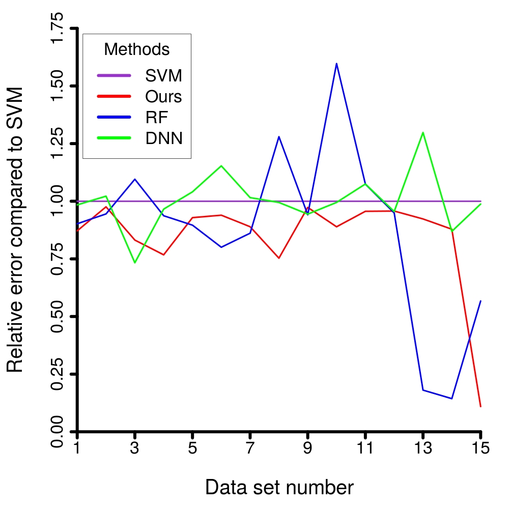
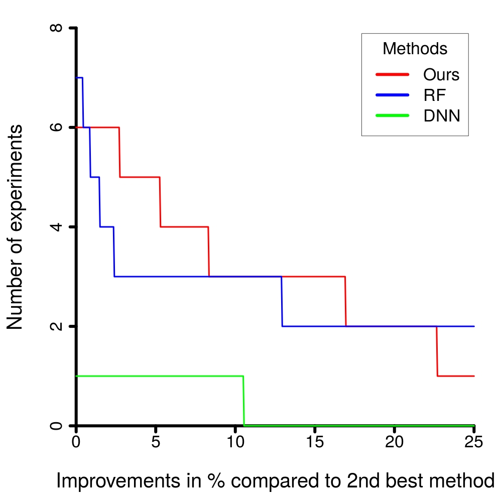
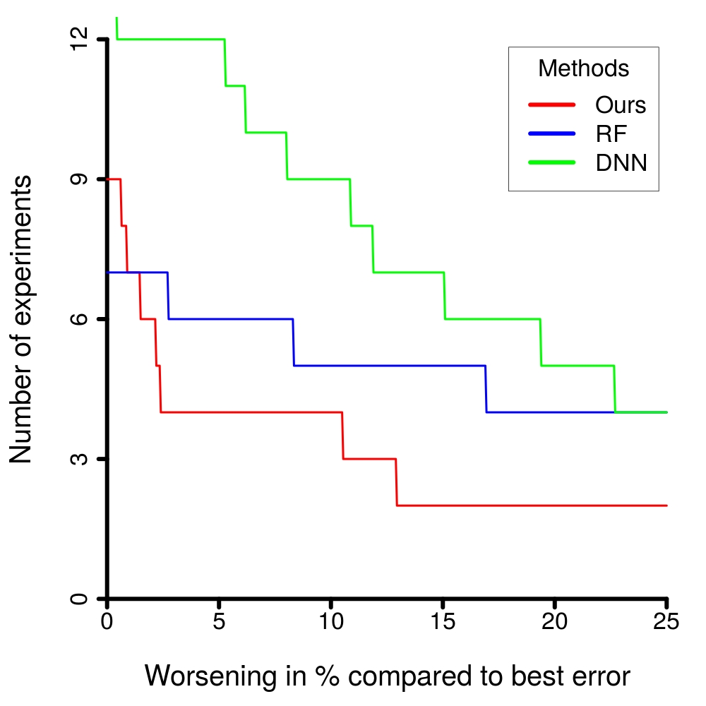
Figure 2: Left. Relative errors of the different algorithms on the 15 data sets. As a baseline, we picked SVMs, that is, the relative error of, say RFs, on a data set is the ratio error(RF)/error(SVM). The figure shows that SVMs and DNNs performed equally well, and that our algorithm consistently outperformed SVMs. The latter is not surprising, since this was the initial intention of our construction. The figure also shows that RFs and DNNs have a quite complementary performance: on most data sets on which RFs performed better than the SVM, the DNNs did not, and vice versa. Middle. This graphic compares our algorithm to RFs and DNNs from a different angle. It shows, for example, that our algorithm achieved a 5% better average risk than the other two algorithms on 5 data sets, while RFs and DNNs did so on 3 and 1 data sets, respectively. This graphic therefore illustrates the potential gain of using one of the algorithms. Right. This graphic illustrates the potential risk of solely using one of the three algorithms. For example, it shows that our algorithm achieved an error that was 10% worse than the best error on 4 data sets, while RFs and DNNs did so on 5 and 9 data sets, respectively.

Data. We downloaded 15 data sets from the UCI Machine Learning Repository and from LIBSVM’s web page, where we note that some data sets can actually be found on both sites. In all cases, we scaled the input variables $x$ to $[-1,1]^{d}$ and the label $y$ to $[-1,1]$. We randomly generated 30 training and test sets from these data sets, where the training set size ranged from 5.000 to 7.000 samples. The details of the considered data sets as well as their preparation are summarized in Table 2 in the appendix.

Execution. All experiments were repeated 30 times, so that every algorithm was run 450 times. These runs were distributed among several computers with different hardware: The RF- and SVM-experiments were conducted on an ordinary desktop computer, where each RF run took between 5 and 60 seconds, and an average SVM run took about 60 seconds. The DNN runs were conducted on a PC with an i7-3930K processor, 64GB of RAM and a Titan GPU. Here, the average experiment ran for about 45 minutes. The runs for our algorithm were distributed among 4 identical PCs with an i7-5820K processor, 64GB of RAM and a GTX980 GPU. On average, a single run took about 81 minutes, but some control experiments on the PC with the Titan GPU showed that on that machine an average run would have taken around 45 minutes, too. In addition note, that the DNNs were using single precision while our algorithm was using double precision, which is between 2 to 3 times slower on the Titan. Finally, the HKL experiments were run on 10 PCs with i7-3770 processor and 16GB of RAM, and an average run took about 60 minutes. Altogether, we used more than 1.400 hours, or 58.4 days, of processing time, which indicates that the experiments would have been infeasible without distributing the tasks among heterogeneous hardware.

Results. The average least squares error for each algorithm and data set can be found, together with some preliminary ranking of the algorithms, in Table 1. A quick look shows that both our method and RFs consistently performed well, scoring on 14, respectively 11, data sets among the top two, which are typeset in bold face. Moreover, our algorithm scored first on 6 data sets, while RFs scored best on 7. The algorithm with the next best scoring is DNN, although this impression is a bit biased since the SVMs were outperformed by our algorithm, as intended, on every single data set, so that the SVMs had never a chance to score first. A somewhat better comparison between DNNs and SVMs can thus be found in the left graphic of Figure 2, which shows that both algorithms perform quite comparable. Finally, we were quite surprised by the performance of HKL, which never scored first or second. Despite this small issue let us finally have a look at a slightly finer comparison between RFs, DNNs and our algorithm, which can be found in Figure 2, middle and right. Here it turns out that the majority of wins for RFs were only achieved by a small improvement compared to the second best among these three algorithm, while our algorithm achieves many of its victories with a larger margin. For example, RFs won on 3 data sets by more than 5% improvement, DNNs on 1, and our algorithm even on 5. In this respect we finally note, that RFs dramatically outperformed all other methods on two data sets, namely shuttle, thyroid, while our algorithm did so on updrs. Last but not least, the graphic on the right hand side of Figure 2 shows on how many data sets each of the three considered algorithms lack behind the best algorithm by which percentage. For example, RFs are 5% worse than the best algorithm on 5 data sets, DNNs on 9, and our algorithm on 4.

A Appendix

Lemma A.1.

For a kernel $k$ on $X$ the following statements are equivalent:

1. $k$ is injective.

2. $k$ has one injective feature map.

3. All feature maps of $k$ are injective.

Proof of Lemma A.1: The implications $iii)\Rightarrow i)\Rightarrow ii)$ are trivial. To show the remaining implication, let $\Phi_{0}:X\to H_{0}$ be an arbitrary feature map of $k$ and $\Phi_{1}:X\to H_{1}$ be an injective feature map of $k$. For $x,x^{\prime}$ we then have

$$\|\Phi_{0}(x)-\Phi_{0}(x^{\prime})\|_{H_{0}}^{2}=k(x,x)-2k(x,x^{\prime})+k(x^{\prime},x^{\prime})=\|\Phi_{1}(x)-\Phi_{1}(x^{\prime})\|_{H_{1}}^{2}\,,$$

that is $\Phi_{0}(x)=\Phi_{0}(x^{\prime})$ if and only if $\Phi_{1}(x)=\Phi_{1}(x^{\prime})$, and by assumption the latter is equivalent to $x=x^{\prime}$. ∎

Theorem A.2.

Let $X$ be a compact metric space and $k$ be a continuous and injective kernel with feature map $\Phi:X\to H$ and feature space $H$, then $k_{\gamma,X,H}$ defined by (2) is a universal kernel.

Proof of Theorem A.2: Since $\|\Phi(x)-\Phi(x^{\prime})\|_{H}^{2}=k(x,x)-2k(x,x^{\prime})+k(x^{\prime},x^{\prime})$ we may assume without loss of generality that $H$ is the RKHS of $k$ and $\Phi$ is the canonical feature map of $k$. Now every compact metric space is separable and since we assumed that $k$ is continuous, we see by [14, Lemma 4.33] that $H$ is separable. Moreover, the continuity of $k$ implies the continuity of $\Phi$, see [14, Lemma 4.29], and consequently, the assertion follows from [4, Theorem 2.2]. ∎

Lemma A.3.

Let $k$ be a kernel of the form (3) and $H$ be its RKHS. Then the resulting hierarchical Gaussian kernel $k_{\gamma,X_{I},H}$ can be computed by

$$k_{\gamma,X_{I},H}(x,x^{\prime})=\prod_{i=1}^{l}k_{\gamma/w_{i},X,H_{i}}\bigl{(}x_{I_{i}},x^{\prime}_{I_{i}}\bigr{)}\,,\qquad\qquad x,x^{\prime}\in X_{I}.$$

Proof of Lemma A.3: Let $\Phi:X_{I}\to H$ be the canonical feature map of $k$, and $\Phi_{i}:X_{I_{i}}\to H_{i}$ be the canonical feature map of $k_{i}$. Then a simple calculation shows that, for all $x,x^{\prime}\in X_{I}$, we have

$$k_{\gamma,X_{I},H}(x,x^{\prime})$$

$$=\exp\bigl{(}-\gamma^{-2}\|\Phi(x)-\Phi(x^{\prime})\|_{H}^{2}\bigr{)}$$

$$=\exp\bigl{(}-\gamma^{-2}k(x,x)+2\gamma^{-2}k(x,x^{\prime})-\gamma^{-2}k(x^{\prime},x^{\prime})\bigr{)}$$

$$=\exp\biggl{(}-\gamma^{-2}\sum_{i=1}^{l}w_{i}^{2}k_{i}\bigl{(}x_{I_{i}},x_{I_{i}}\bigr{)}+2\gamma^{-2}\sum_{i=1}^{l}w_{i}^{2}k_{i}\bigl{(}x_{I_{i}},x^{\prime}_{I_{i}}\bigr{)}-\gamma^{-2}\sum_{i=1}^{l}w_{i}^{2}k_{i}\bigl{(}x^{\prime}_{I_{i}},x^{\prime}_{I_{i}}\bigr{)}\biggr{)}$$

$$=\exp\biggl{(}-\gamma^{-2}\sum_{i=1}^{l}w_{i}^{2}\Bigl{(}k_{i}\bigl{(}x_{I_{i}},x_{I_{i}}\bigr{)}-2k_{i}\bigl{(}x_{I_{i}},x^{\prime}_{I_{i}}\bigr{)}+k_{i}\bigl{(}x^{\prime}_{I_{i}},x^{\prime}_{I_{i}}\bigr{)}\Bigr{)}\biggr{)}$$

$$=\exp\biggl{(}-\gamma^{-2}\sum_{i=1}^{l}w_{i}^{2}\bigl{\|}\,\Phi_{i}(x_{I_{i}})-\Phi_{i}(x^{\prime}_{I_{i}})\,\bigr{\|}_{H_{i}}^{2}\biggr{)}$$

$$=\prod_{i=1}^{l}\exp\biggl{(}-\gamma^{-2}w_{i}^{2}\bigl{\|}\,\Phi_{i}(x_{I_{i}})-\Phi_{i}(x^{\prime}_{I_{i}})\,\bigr{\|}_{H_{i}}^{2}\biggr{)}$$

$$=\prod_{i=1}^{l}k_{\gamma/w_{i},X,H_{i}}\bigl{(}x_{I_{i}},x^{\prime}_{I_{i}}\bigr{)}\,.$$

In other words, we have shown the assertion. ∎

Theorem A.4.

Let $k$ be a kernel of the form (3) and $H$ be its RKHS. If all kernels $k_{1},\dots,k_{l}$ are injective, and $X_{I}$ is compact, then the resulting hierarchical Gaussian kernel $k_{\gamma,X_{I},H}$ is universal.

Proof of Theorem A.4: By Theorem A.2 and the assumed injectivity of $k_{i}$ we know that $k_{\gamma/w_{i},X_{i},H_{i}}$ is universal on $X_{I_{i}}$. Moreover, Lemma A.3 shows that

$$k_{\gamma,X,H}(x,x^{\prime})=\prod_{i=1}^{l}k_{\gamma/w_{i},X,H_{i}}\bigl{(}x_{I_{i}},x^{\prime}_{I_{i}}\bigr{)}\,,\qquad\qquad x,x^{\prime}\in X.$$

Therefore, Lemma A.5 together with a simple induction over $l$ gives the desired result. ∎

Lemma A.5.

Let $X\subset\mathbb{R}^{m}$ be a compact and non-empty subset, $I,J\subset\{1,\dots,m\}$ be non-empty, and $k_{I}$ and $k_{J}$ be universal kernels on $X_{I}$ and $X_{J}$, respectively. Then $k_{I}\otimes k_{J}$ defined by

$$k_{I}\otimes k_{J}(x,x^{\prime}):=k_{I}(x_{I},x^{\prime}_{I})\cdot k_{J}(x_{J},x^{\prime}_{J})$$

for all $x,x^{\prime}\in X_{I\cup J}$ is a universal kernel on $X_{I\cup J}$.

Proof of Lemma A.5: Let us denote the RKHSs of $k_{I}$ and $k_{J}$ by $H_{I}$ and $H_{J}$, respectively. Similarly, we write $\Phi_{I}$ and $\Phi_{J}$ for the canonical feature maps of these kernels. Moreover, let $H_{I}\otimes H_{J}$ be the formal tensor product of $H_{I}$ and $H_{J}$. Recall that this tensor product is a vector space spanned by the elementary tensors $h_{I}\otimes h_{J}$, where $h_{I}\in H_{I}$ and $h_{J}\in H_{J}$. Moreover, there is a unique inner product $\langle\,\cdot\,,\,\cdot\,\rangle_{H_{I}\otimes H_{J}}$ on $H_{I}\otimes H_{J}$ that satisfies

$$\langle h_{I}\otimes h_{J},h^{\prime}_{I}\otimes h^{\prime}_{J}\rangle_{H_{I}\otimes H_{J}}=\langle h_{I},h^{\prime}_{I}\rangle_{H_{I}}\cdot\langle h_{J},h^{\prime}_{J}\rangle_{H_{J}}$$

for all elementary tensors. We write $H_{I}\hat{\otimes}H_{J}$ for the completion of $H_{I}\otimes H_{J}$ with respect to the norm resulting from $\langle\,\cdot\,,\,\cdot\,\rangle_{H_{I}\otimes H_{J}}$. Then the map

$$\Phi_{I}\otimes\Phi_{J}:X_{I\cup J} \to H_{I}\hat{\otimes}H_{J}$$

$$x \mapsto\Phi_{I}(x_{I})\otimes\Phi_{J}(x_{J})$$

is a feature map of $k_{I}\otimes k_{J}$ since for $x,x^{\prime}\in X_{I\cup J}$ we have

$$\bigl{\langle}\Phi_{I}\otimes\Phi_{J}(x),\Phi_{I}\otimes\Phi_{J}(x^{\prime})\bigr{\rangle}_{H_{I}\hat{\otimes}H_{J}} =\bigl{\langle}\Phi_{I}(x_{I})\otimes\Phi_{J}(x_{J}),\Phi_{I}(x^{\prime}_{I})\otimes\Phi_{J}(x^{\prime}_{J})\bigr{\rangle}_{H_{I}\otimes H_{J}}$$

$$=\bigl{\langle}\Phi_{I}(x_{I}),\Phi_{I}(x^{\prime}_{I})\bigr{\rangle}_{H_{I}}\cdot\bigl{\langle}\Phi_{J}(x_{J}),\Phi_{J}(x^{\prime}_{J})\bigr{\rangle}_{H_{J}}$$

$$=k_{I}(x_{I},x^{\prime}_{I})\cdot k_{J}(x_{J},x^{\prime}_{J})$$

$$=k_{I}\otimes k_{J}(x,x^{\prime})\,.$$

By [14, Theorem 4.21] we then know that the RKHS $H$ of $k_{I}\otimes k_{J}$ is given by

$$H=\Bigl{\{}h:X_{I\cup J}\to\mathbb{R}\,\bigl{|}\,\exists v\in H_{I}\hat{\otimes}H_{J}\mbox{ with }h(x)=\bigl{\langle}v,\Phi_{I}\otimes\Phi_{J}(x)\bigr{\rangle}_{H_{I}\hat{\otimes}H_{J}}\mbox{ for all $x\in X_{I\cup J}$}\Bigr{\}}\,.$$

Now observe that $k_{I}$ and $k_{J}$ are continouos because of their assumed universality and therefore, $k_{I}\otimes k_{J}$ is continuous, too. In particular, $H$ consists of continuous functions.

Let us now consider the space

$$C(X_{I})\otimes C(X_{J}):=\operatorname{span}\bigl{\{}f\otimes g\,\bigl{|}\,f\in C(X_{I}),\,g\in C(X_{J})\bigr{\}}\,,$$

where again we define the functions $f\otimes g:X_{I\cup J}\to\mathbb{R}$ by $f\otimes g(x):=f(x_{I})\cdot g(x_{J})$ for all $x\in X_{I\cup J}$. Our next goal is to show that $H$ approximates the space $C(X_{I})\otimes C(X_{J})$ arbitrarily well with respect to the $\|\cdot\|_{\infty}$, that is

$$C(X_{I})\otimes C(X_{J})\subset\overline{H}^{\|\cdot\|_{\infty}}\,,$$ (12)

where $\overline{H}^{\|\cdot\|_{\infty}}$ denotes the $\|\cdot\|_{\infty}$-closure of $H$ in $C(X_{I\cup J})$. To this end, it clearly suffices to show that each $f\otimes g\in C(X_{I})\otimes C(X_{J})$ can be arbitrarily well approximated. To show the latter, we fix an $\varepsilon>0$. Since $k_{I}$ and $k_{J}$ are universal, there then exist $h_{I}\in H_{I}$ and $h_{J}\in H_{J}$ with $\|h_{I}-f\|_{\infty}\leq\varepsilon$ and $\|h_{J}-g\|_{\infty}\leq\varepsilon$. For the function $h\in H$ defined by $h(x):=\bigl{\langle}h_{I}\otimes h_{J},\Phi_{I}\otimes\Phi_{J}(x)\bigr{\rangle}_{H_{I}\hat{\otimes}H_{J}}$ we then have

$$h(x)=\bigl{\langle}h_{I}\otimes h_{J},\Phi_{I}\otimes\Phi_{J}(x)\bigr{\rangle}_{H_{I}\hat{\otimes}H_{J}}=\bigl{\langle}h_{I},\Phi_{I}(x_{I})\bigr{\rangle}_{H_{I}}\cdot\bigl{\langle}h_{J},\Phi_{J}(x_{J})\bigr{\rangle}_{H_{J}}=h_{I}(x_{I})\cdot h_{J}(x_{J})$$

for all $x\in X_{I\cup J}$. This equation together with $\|h_{J}\|_{\infty}-\|g\|_{\infty}\leq\|h_{J}-g\|_{\infty}\leq\varepsilon$ now gives

$$\|h-f\otimes g\|_{\infty}=\|h_{I}h_{J}-fg\|_{\infty} \leq\|h_{I}h_{J}-fh_{J}\|_{\infty}+\|fh_{J}-fg\|_{\infty}$$

$$\leq\|h_{I}-f\|_{\infty}\cdot\|h_{J}\|_{\infty}+\|f\|_{\infty}\cdot\|h_{J}-g\|_{\infty}$$

$$\leq\varepsilon\cdot(\|g\|_{\infty}+\varepsilon)+\|f\|_{\infty}\cdot\varepsilon\,.$$

From the latter we easily conclude that (A) holds.

In view of (A) we now show in the last step of the proof that ${\cal A}:=C(X_{I})\otimes C(X_{J})$ is dense in $C(X_{I\cup J})$. To this end, we first observe that ${\cal A}$ is a sub-algebra of $C(X_{I\cup J})$ by construction. Moreover, ${\cal A}$ does not vanish, since for $x\in X_{I\cup J}$ there exist $f\in C(X_{I})$ and $g\in C(X_{J})$ with $f(x_{I})\neq 0$ and $g(x_{J})\neq 0$. This gives $f\otimes g(x)=f(x_{I})\cdot g(x_{J})\neq 0$. Finally, ${\cal A}$ also separates points. To check this, we first observe that for $x,x^{\prime}\in X_{I\cup J}$ with $x\neq x^{\prime}$ we have $x_{I}\neq x_{I}^{\prime}$ or $x_{J}\neq x^{\prime}_{J}$. Let us assume without loss of generality that $x_{I}\neq x_{I}^{\prime}$. Then there exists an $f\in C(X_{I})$ with $f(x_{I})\neq f(x^{\prime}_{J})$. For $g:=\boldsymbol{1}_{X_{J}}\in C(X_{J})$ being the constant one function, we then obtain $f\otimes g(x)=f(x_{I})\neq f(x^{\prime}_{I})=f\otimes g(x^{\prime})$, and therefore ${\cal A}$ does separate points. By the theorem of Stone-Weierstraß we then see that ${\cal A}$ is dense in $C(X_{I\cup J})$. ∎

Lemma A.6.

Let $k$ be a kernel of the form (3) and $H$ be its RKHS. Then the resulting hierarchical Gaussian kernel $k_{\gamma,X_{I},H}$ satisfies

$$\frac{\partial}{\partial w_{j}}k_{\gamma,X_{I},H}(x,x^{\prime})=-2w_{j}\gamma^{-2}\bigl{\|}\,\Phi_{j}(x_{I_{j}})-\Phi_{j}(x^{\prime}_{I_{j}})\,\bigr{\|}_{H_{j}}^{2}k_{\gamma,X_{I},H}(x,x^{\prime})\,,\qquad\qquad x,x^{\prime}\in X.$$

Proof of Lemma A.6: Using Lemma A.3 we find

$$\frac{\partial}{\partial w_{j}}k_{\gamma,X_{I},H}(x,x^{\prime}) =\frac{\partial}{\partial w_{j}}\prod_{i=1}^{l}k_{\gamma/w_{i},X,H_{i}}\bigl{(}x_{I_{i}},x^{\prime}_{I_{i}}\bigr{)}$$

$$=\prod_{i\neq j}k_{\gamma/w_{i},X,H_{i}}\bigl{(}x_{I_{i}},x^{\prime}_{I_{i}}\bigr{)}\cdot\frac{\partial}{\partial w_{j}}k_{\gamma/w_{j},X,H_{j}}\bigl{(}x_{I_{j}},x^{\prime}_{I_{j}}\bigr{)}\,.$$

Moreover, we have

$$\frac{\partial}{\partial w_{j}}k_{\gamma/w_{j},X,H_{j}}\bigl{(}x_{I_{j}},x^{\prime}_{I_{j}}\bigr{)}$$

$$=\frac{\partial}{\partial w_{j}}\exp\biggl{(}-\gamma^{-2}w_{j}^{2}\bigl{\|}\,\Phi_{j}(x_{I_{j}})-\Phi_{j}(x^{\prime}_{I_{j}})\,\bigr{\|}_{H_{j}}^{2}\biggr{)}$$

$$=-2\gamma^{-2}w_{j}\bigl{\|}\,\Phi_{j}(x_{I_{j}})-\Phi_{j}(x^{\prime}_{I_{j}})\,\bigr{\|}_{H_{j}}^{2}\exp\biggl{(}-\gamma^{-2}w_{j}^{2}\bigl{\|}\,\Phi_{j}(x_{I_{j}})-\Phi_{j}(x^{\prime}_{I_{j}})\,\bigr{\|}_{H_{j}}^{2}\biggr{)}$$

$$=-2\gamma^{-2}w_{j}\bigl{\|}\,\Phi_{j}(x_{I_{j}})-\Phi_{j}(x^{\prime}_{I_{j}})\,\bigr{\|}_{H_{j}}^{2}k_{\gamma/w_{j},X,H_{j}}\bigl{(}x_{I_{j}},x^{\prime}_{I_{j}}\bigr{)}\,,$$

and by combining both expressions we obtain the assertion. ∎

Proof of Lemma 4.1: Let $H_{j}$ be a RKHS of $k_{\mathbf{W}^{(1)}_{j},\dots,\mathbf{W}^{(m-2)}_{j},\mathbf{w}_{j}^{(m-1)}}$ and $\Phi_{j}$ be the corresponding canonical feature map. Then the formula for the highest layer follows from Lemma A.6 and

$$\bigl{\|}\,\Phi_{j}(x_{I_{j}})-\Phi_{j}(x^{\prime}_{I_{j}})\,\bigr{\|}_{H_{j}}^{2}=2-2k_{\mathbf{W}^{(1)}_{j},\dots,\mathbf{W}^{(m-2)}_{j},\mathbf{w}_{j}^{(m-1)}}(x_{I_{j}},x_{I_{j}}^{\prime})\,.$$

Moreover, if $w$ is a weight that occurs in a lower layer of the $j$-th node, that is, it occurs at the component $\mathbf{W}^{(n)}_{j}$ of $\mathbf{W}^{(n)}$ for some $n\leq m-1$, then (7) gives

$$\frac{\partial}{\partial w}k_{\mathbf{W}^{(1)},\dots,\mathbf{W}^{(m-1)},\mathbf{w},\gamma}(x,x^{\prime}) =\frac{\partial}{\partial w}\exp\biggl{(}\!\!-2\gamma^{-2}\sum_{i=1}^{l}w_{i}^{2}\bigl{(}1\!-\!k_{\mathbf{W}^{(1)}_{i},\dots,\mathbf{W}^{(m-2)}_{i},\mathbf{w}_{i}^{(m-1)}}(x_{I_{i}},x^{\prime}_{I_{i}})\bigr{)}\!\!\biggr{)}$$

$$=\exp\biggl{(}-2\gamma^{-2}\sum_{i\neq j}w_{i}^{2}\bigl{(}1-k_{\mathbf{W}^{(1)}_{i},\dots,\mathbf{W}^{(m-2)}_{i},\mathbf{w}_{i}^{(m-1)}}(x_{I_{i}},x^{\prime}_{I_{i}})\bigr{)}\biggr{)}$$

$$\quad\cdot\frac{\partial}{\partial w}\exp\biggl{(}\!-2\gamma^{-2}w_{j}^{2}\bigl{(}1-k_{\mathbf{W}^{(1)}_{j},\dots,\mathbf{W}^{(m-2)}_{j},\mathbf{w}_{j}^{(m-1)}}(x_{I_{j}},x^{\prime}_{I_{j}})\bigr{)}\!\biggr{)}\,.$$

In addition, the chain rule yields

$$\frac{\partial}{\partial w}\exp\biggl{(}\!-2\gamma^{-2}w_{j}^{2}\bigl{(}1-k_{\mathbf{W}^{(1)}_{j},\dots,\mathbf{W}^{(m-2)}_{j},\mathbf{w}_{j}^{(m-1)}}(x_{I_{j}},x^{\prime}_{I_{j}})\bigr{)}\!\biggr{)}$$

$$=\exp\biggl{(}\!-2\gamma^{-2}w_{j}^{2}\bigl{(}1-k_{\mathbf{W}^{(1)}_{j},\dots,\mathbf{W}^{(m-2)}_{j},\mathbf{w}_{j}^{(m-1)}}(x_{I_{j}},x^{\prime}_{I_{j}})\bigr{)}\!\biggr{)}$$

$$\quad\cdot\frac{\partial}{\partial w}\Bigl{(}-2\gamma^{-2}w_{j}^{2}\bigl{(}1-k_{\mathbf{W}^{(1)}_{j},\dots,\mathbf{W}^{(m-2)}_{j},\mathbf{w}_{j}^{(m-1)}}(x_{I_{j}},x^{\prime}_{I_{j}})\bigr{)}\Bigr{)}$$

$$=\exp\biggl{(}\!-2\gamma^{-2}w_{j}^{2}\bigl{(}1-k_{\mathbf{W}^{(1)}_{j},\dots,\mathbf{W}^{(m-2)}_{j},\mathbf{w}_{j}^{(m-1)}}(x_{I_{j}},x^{\prime}_{I_{j}})\bigr{)}\!\biggr{)}$$

$$\quad\cdot 2\gamma^{-2}w_{j}^{2}\frac{\partial}{\partial w}k_{\mathbf{W}^{(1)}_{j},\dots,\mathbf{W}^{(m-2)}_{j},\mathbf{w}_{j}^{(m-1)}}(x_{I_{j}},x^{\prime}_{I_{j}})\,.$$

Combining both expressions, we then obtain the second formula. ∎

To illustrate the lemma 4.1 we note that the parameter derivatives of hierarchical Gaussians $k_{\mathbf{v}}$ of depth 1, that is, of kernels of the form (4), are given by

$$\frac{\partial}{\partial v_{j}}k_{\mathbf{v}}(x,x^{\prime})=-2v_{j}(x_{j}-x_{j}^{\prime})^{2}k_{\mathbf{v}}(x,x^{\prime})\,,\qquad\qquad x,x^{\prime}\in X\,.$$

To derive an explicit formula for depth-2-kernels we fix some first layer weight vectors $\mathbf{v}_{1}=(v_{i,1})_{i\in I_{1}},\dots,\mathbf{v}_{l}=(v_{i,l})_{i\in I_{l}}$ and a second layer weight vector $\mathbf{w}=(w_{1},\dots w_{l})$. Let us write $\mathbf{V}:=\mathbf{W}^{(1)}:=(\mathbf{v}_{1},\dots\mathbf{v}_{l})$. The first formula of Lemma 4.1 then shows that the depth-2 kernel $k_{\mathbf{V},\mathbf{w},\gamma}$ defined in (5) has the $\mathbf{w}$-parameter derivatives

$$\frac{\partial}{\partial w_{j}}k_{\mathbf{V},\mathbf{w},\gamma}(x,x^{\prime})=-4w_{j}\gamma^{-2}\bigl{(}1-k_{\mathbf{v}_{j}}(x,x^{\prime})\bigr{)}k_{\mathbf{V},\mathbf{w},\gamma}(x,x^{\prime})\,.$$

Moreover, the second formula of Lemma 4.1 gives

$$\frac{\partial}{\partial v_{i,j}}k_{\mathbf{V},\mathbf{w},\gamma}(x,x^{\prime})=2\gamma^{-2}w_{j}^{2}\frac{\partial}{\partial v_{i,j}}k_{\mathbf{v}_{j}}(x,x^{\prime})=-4v_{i,j}\gamma^{-2}w_{j}^{2}(x_{j}-x_{j}^{\prime})^{2}k_{\mathbf{v}_{j}}(x,x^{\prime})\,.$$

Data Set	Size	Dimension.	Type	Training	Testing	Source
Bank-Marketing	45211	16	BC	7000	24212	UCI
Cadata	20640	8	REG	7000	6640	LIBSVM
Cod-rna	331152	8	BC	7000	310154	LIBSVM
Covtype	581012	55	BC	7000	560014	UCI
Cpusmall	8192	12	REG	6000	2192	LIBSVM
Cycle-Power-Plant	9568	4	REG	6000	3568	UCI
Higgs	500000	28	BC	7000	479002	UCI
Letter-Recognition	20000	16	MC-26	7000	6000	UCI
Magic	19020	10	BC	7000	5022	UCI
Pendigits	10992	16	MC-10	7000	3992	UCI
Satimage	6435	36	MC-6	5000	1435	UCI
Seismic	98528	50	MC-3	7000	77530	LIBSVM
Shuttle	43500	8	MC-6	7000	22500	LIBSVM
Thyroid-ann	7200	21	BC	5000	2001	UCI
Updrs-motor	5875	19	REG	5000	875	UCI

Table 2: Details of the considered datasets and their preparation. All data sets were scaled to $[-1,1]^{d+1}$ or $[0,1]$. For Shuttle we additionally removed the first data column that contains a time stamp whose influence has been debated in the literature. The types are binary classification (BC), regression (REG), and multiclass classification with $k$ labels (MC-$k$). We subsampled training and test sets of the specified size. For the larger datasets we initially planned some additional experiments, for which a separate data set would have been needed. This explains the difference between the total size and the sum of the training and test set sizes. These splits were 30 times repeated.

References

• [1] F. R. Bach. Exploring large feature spaces with hierarchical multiple kernel learning. In D. Koller, D. Schuurmans, Y. Bengio, and L. Bottou, editors, Advances in Neural Information Processing Systems 21, pages 105–112. 2008.
• [2] J. F. Bonnans, J. C. Gilbert, C. Lemaréchal, and C. A. Sagastizábal. Numerical Optimization: Theoretical and Practical Aspects. Springer-Verlag, Berlin, 2nd edition, 2006.
• [3] Y. Cho and L.K. Saul. Kernel methods for deep learning. In Y. Bengio, D. Schuurmans, J.D. Lafferty, C.K.I. Williams, and A. Culotta, editors, Advances in Neural Information Processing Systems 22, pages 342–350. 2009.
• [4] A. Christmann and I. Steinwart. Universal kernels on non-standard input spaces. In J. Lafferty, C. K. I. Williams, J. Shawe-Taylor, R.S. Zemel, and A. Culotta, editors, Advances in Neural Information Processing Systems 23, pages 406–414, 2010.
• [5] F. Cucker and D. X. Zhou. Learning Theory: An Approximation Theory Viewpoint. Cambridge University Press, Cambridge, 2007.
• [6] M. Eberts and I. Steinwart. Optimal regression rates for SVMs using Gaussian kernels. Electron. J. Stat., 7:1–42, 2013.
• [7] M. Fernández-Delgado, E. Cernadas, S. Barro, and D. Amorim. Do we need hundreds of classifiers to solve real world classification problems? J. Mach. Learn. Res., 15:3133–3181, 2014.
• [8] Y. Jia, E. Shelhamer, J. Donahue, S. Karayev, J. Long, R. Girshick, S. Guadarrama, and T. Darrell. Caffe: Convolutional architecture for fast feature embedding. arXiv preprint arXiv:1408.5093, 2014.
• [9] J. Mairal, P. Koniusz, Z. Harchaoui, and C. Schmid. Convolutional Kernel Networks. In Advances in Neural Information Processing Systems, 2014.
• [10] W. H. Press, S. A. Teukolskyand W. T. Vetterling, and B. P. Flannery. Numerical Recipes: The Art of Scientific Computing. Cambridge University Press, Cambridge, 3rd edition, 2007.
• [11] S. Smale and D.-X. Zhou. Estimating the approximation error in learning theory. Anal. Appl., 1:17–41, 2003.
• [12] S. Sonnenburg, G. Rätsch, C. Schäfer, and B. Schölkopf. Large scale multiple kernel learning. J. Mach. Learn. Res., 7:1531–1565, 2006.
• [13] I. Steinwart. A fast SVM toolbox. http://www.isa.uni-stuttgart.de/software/, January 2016.
• [14] I. Steinwart and A. Christmann. Support Vector Machines. Springer, New York, 2008.
• [15] E.V. Strobl and S. Visweswaran. Deep multiple kernel learning. In Machine Learning and Applications (ICMLA), 2013 12th International Conference on, volume 1, pages 414–417, 2013.
• [16] Yichuan Tang. Deep learning using support vector machines. In ICML 2013 Challenges in Representation Learning Workshop, 2013.
• [17] A.G. Wilson, Z. Hu, R. Salakhutdinov, and E.P. Xing. Deep kernel learning. JMLR W&CP, 51:370–378, 2016.
• [18] J. Zhuang, I.W. Tsang, and S. Hoi. Two-layer multiple kernel learning. JMLR W&CP, 15:909–917, 2011.