UH-511-1269-16

Gluino reach and mass extraction at the LHC
in radiatively-driven natural SUSY

Howard Baer¹, Vernon Barger², James S. Gainer³, Peisi Huang^4,5,6,
Michael Savoy¹, Dibyashree Sengupta¹, and Xerxes Tata³

¹Dept. of Physics and Astronomy, University of Oklahoma, Norman, OK 73019, USA
²Dept. of Physics, University of Wisconsin, Madison, WI 53706, USA
³Dept. of Physics, University of Hawaii, Honolulu, HI 96822, USA
⁴Enrico Fermi Institute, University of Chicago, Chicago, IL 60637, USA
⁵HEP Division, Argonne National Laboratory, 9700 Cass Ave., Argonne, IL 60439, USA ⁶Mitchell Institute for Fundamental Physics and Astronomy, Texas A&M University, College Station, TX 77843, USA

Radiatively-driven natural SUSY (RNS) models enjoy electroweak naturalness at the 10% level while respecting LHC sparticle and Higgs mass constraints. Gluino and top squark masses can range up to several TeV (with other squarks even heavier) but a set of light Higgsinos are required with mass not too far above $m_{h}\sim 125$ GeV. Within the RNS framework, gluinos dominantly decay via $\tilde{g}\rightarrow t\tilde{t}_{1}^{*},\ \bar{t}\tilde{t}_{1}\rightarrow t\bar{t}\widetilde{Z}_{1,2}$ or $t\bar{b}\widetilde{W}_{1}^{-}+c.c.$, where the decay products of the higgsino-like $\widetilde{W}_{1}$ and $\widetilde{Z}_{2}$ are very soft. Gluino pair production is, therefore, signalled by events with up to four hard $b$-jets and large $\not\!\!{E_{T}}$. We devise a set of cuts to isolate a relatively pure gluino sample at the (high luminosity) LHC and show that in the RNS model with very heavy squarks, the gluino signal will be accessible for $m_{\tilde{g}}<2400\ (2800)$ GeV for an integrated luminosity of 300 (3000) fb^-1. We also show that the measurement of the rate of gluino events in the clean sample mentioned above allows for a determination of $m_{\tilde{g}}$ with a statistical precision of 2.5-5% (depending on the integrated luminosity and the gluino mass) over the range of gluino masses where a 5$\sigma$ discovery is possible at the LHC.

1 Introduction

Supersymmetric (SUSY) models of particle physics are strongly motivated because they provide a solution to the gauge hierarchy problem (GHP) [1] which arises when the spin zero Higgs sector of the Standard Model (SM) is coupled to a high mass sector as, for instance, in a Grand Unified Theory (GUT). SUSY models are indirectly supported by data in that (1) the measured values of the three gauge coupling strengths unify in the minimal supersymmetrized Standard Model (MSSM) [2], (2) the top-quark mass is measured to lie in the range required by SUSY to trigger a radiative breakdown of electroweak symmetry [3], and (3) the measured value of the Higgs boson mass [4] lies squarely within the range required by the MSSM [5]. However, so far no unambiguous signal for superparticles has emerged from LHC searches [6]. In the case of the gluino, $\tilde{g}$, (the spin-$1/2$ superpartner of the gluon), recent search results in the context of simplified models place mass limits as high as $m_{\tilde{g}}\stackrel{{\scriptstyle>}}{{\sim}}1500-1900$ GeV [7, 8] for a massless lightest SUSY particle (LSP), depending on the assumed decay of the gluino. This may be contrasted with early expectations from naturalness, such as the Barbieri-Giudice (BG) $\Delta_{\rm BG}<30$ bounds [9], which required $m_{\tilde{g}}\stackrel{{\scriptstyle<}}{{\sim}}350$ GeV.

Likewise, LHC simplified model analyses typically require $m_{\tilde{t}_{1}}\stackrel{{\scriptstyle>}}{{\sim}}700-850$ GeV [8, 11] to be contrasted with Dimopoulos-Giudice (DG) $\Delta_{BG}<30$ fine-tuning bounds [12] that require $m_{\tilde{t}_{1}}\stackrel{{\scriptstyle<}}{{\sim}}500$ GeV or with Higgs mass large log bounds [13] which require three third generation squarks of mass $\stackrel{{\scriptstyle<}}{{\sim}}500$ GeV. Conflicts such as these have led many to question whether weak scale SUSY is indeed nature’s chosen solution to the GHP, or whether nature follows some entirely different direction [14].

A more conservative approach to naturalness has been adopted in Refs. [15, 16]. Here, one requires that there are no large cancellations among the various terms on the right hand side of the well-known expression that yields the measured value of $m_{Z}$ in terms of the weak scale SUSY Lagrangian parameters via the scalar potential minimization condition:

$$\frac{m_{Z}^{2}}{2}=\frac{m_{H_{d}}^{2}+\Sigma_{d}^{d}-(m_{H_{u}}^{2}+\Sigma_{u}^{u})\tan^{2}\beta}{\tan^{2}\beta-1}-\mu^{2}\simeq-m_{H_{u}}^{2}-\Sigma_{u}^{u}-\mu^{2}.$$ (1)

The $\Sigma_{u}^{u}$ and $\Sigma_{d}^{d}$ terms in Eq. (1) arise from 1-loop corrections to the scalar potential (expressions can be found in the Appendix of Ref. [16]), $m_{H_{u}}^{2}$ and $m_{H_{d}}^{2}$ are the soft SUSY breaking Higgs mass parameters, $\tan\beta\equiv\langle H_{u}\rangle/\langle H_{d}\rangle$ is the ratio of the Higgs field VEVs and $\mu$ is the superpotential (SUSY conserving) Higgs/higgsino mass parameter. SUSY models requiring large cancellations between the various terms on the right-hand-side of Eq. (1) to reproduce the measured value of $m_{Z}^{2}$ are regarded as unnatural, or fine-tuned. Thus, the electroweak naturalness measure, $\Delta_{\rm EW}$, is given by the maximum value of the ratio of each term on the right-hand-side of Eq. (1) and $m_{Z}^{2}/2$.

This conservative approach to naturalness allows for the possibility that high scale parameters that have been taken to be independent will, in fact, turn out to be correlated once SUSY breaking is understood. Ignoring these correlations will lead to an overestimate of the UV sensitivity of a theory, making it appear to be fine-tuned. In Ref. [17, 18, 19] it is argued that if all correlations among parameters are correctly implemented the conventional Barbieri-Giudice measure reduces to $\Delta_{\rm EW}$ and that a high-scale theory that predicts these parameter correlations would be natural. We urge using the more conservative electroweak measure for discussions of naturalness since disregarding the possibility of parameter correlations may lead to prematurely discarding what may be a perfectly viable effective theory.

For SUSY models with electroweak naturalness, we have:

• $|\mu|\sim 100-300$ GeV (the closer to $m_{Z}$ the more natural) leading to the requirement of four light higgsinos $\widetilde{Z}_{1,2}$ and $\widetilde{W}_{1}^{\pm}$ of similar mass values $\sim|\mu|$,

• $m_{H_{u}}^{2}$ must be driven radiatively to small negative values $\sim-(100-300)^{2}$ GeV² at the weak scale (for this reason, these models are said to exhibit radiatively-driven naturalness, and have been dubbed radiatively-driven natural SUSY (RNS) [15, 16]).

• the radiative corrections $\left|\Sigma_{u}^{u}(i)\right|\stackrel{{\scriptstyle<}}{{\sim}}(100-300)^{2}$ GeV². The largest of these typically arise from the top squarks and require for $\Delta_{\rm EW}<30$ that $m_{\tilde{t}_{1}}\stackrel{{\scriptstyle<}}{{\sim}}3$ TeV, a factor 10 higher than the aforementioned BG/DG bounds. Gluinos contribute to $\Sigma_{u}^{u}$ at two-loop order [21] and in models with gaugino mass unification, then $m_{\tilde{g}}\stackrel{{\scriptstyle<}}{{\sim}}4$ TeV [16, 10, 22].

We see that SUSY models with electroweak naturalness can easily respect LHC sparticle mass bounds and are in accord with the measured value of $m_{h}$, which requires large mixing among top squarks [23].

What of LHC signatures in RNS models? Old favorites like searches for gluino pairs ($pp\rightarrow\tilde{g}\tilde{g}X$ where $X$ represents assorted hadronic debris) are still viable where now $\tilde{g}\rightarrow\tilde{t}_{1}t$ if kinematically allowed or $\tilde{g}\rightarrow t\bar{t}\widetilde{Z}_{i}$ or $t\bar{b}\widetilde{W}_{j}$ when $m_{\tilde{g}}<m_{\tilde{t}_{1}}+m_{t}$ [24]. In the case of RNS, the $m_{\tilde{g}}-m_{\widetilde{Z}_{1}}$ mass gap is expected to be larger than in models such as CMSSM/mSUGRA where the $\widetilde{Z}_{1}$ is typically bino-like. In addition, for RNS, the $\widetilde{Z}_{2}$ produced in gluino cascade decays leads to the presence of opposite-sign/same flavor dilepton pairs with $m(\ell^{+}\ell^{-})<m_{\widetilde{Z}_{2}}-m_{\widetilde{Z}_{1}}\sim 10-20$ GeV [25, 26]. However, new signatures also arise for RNS. Wino pair production $pp\rightarrow\widetilde{W}_{2}\widetilde{Z}_{4}$ can occur at large rates leading to the low background same-sign diboson signature from $\widetilde{W}_{2}\rightarrow W^{+}\widetilde{Z}_{1,2}$ and $\widetilde{Z}_{4}\rightarrow W^{+}\widetilde{W}_{1}^{-}$ decays [25, 27]. This very clean signature leads to the greatest reach for SUSY in the $m_{1/2}$ direction for an integrated luminosity $L\stackrel{{\scriptstyle>}}{{\sim}}100-200$ fb^-1. Also, direct higgsino pair production $pp\rightarrow\widetilde{Z}_{1}\widetilde{Z}_{2}j$ followed by $\widetilde{Z}_{2}\rightarrow\ell^{+}\ell^{-}\widetilde{Z}_{1}$ decay offers substantial reach in the $\mu$ direction of parameter space [28]. Combined, these latter two signatures offer high luminosity (HL) LHC a complete coverage of RNS SUSY with unified gaugino masses for $\Delta_{\rm EW}<30$ and $L\sim 3000$ fb^-1 [29]. In addition to LHC searches, an International Linear $e^{+}e^{-}$ Collider (ILC) with $\sqrt{s}\stackrel{{\scriptstyle>}}{{\sim}}500-600\ {\rm GeV}>2m(higgsino)$ would be a higgsino factory and completely cover the $\Delta_{\rm EW}\leq 30$ RNS parameter space and allow precision measurements that would serve to elucidate the natural origin of $W$, $Z$ and Higgs boson masses [30, 31].

Although the discovery of the gluino at the LHC is not guaranteed over the viable RNS parameter space, we re-examine gluino pair production signatures expected within the RNS framework. Our purpose is first, to delineate the gluino reach of LHC14 and its high-luminosity upgrade, and second, to study the extent to which the gluino mass may be extracted at the LHC. Although not required by naturalness, one usually takes first and second generation matter scalar mass parameters, assumed unified to a value $m_{0}$ at scale $Q=m_{GUT}$, to be in the multi-TeV range. This alleviates the SUSY flavour problem with little impact on naturalness as long as these scalars satisfy well-motivated intra-generational degeneracy patterns [32]. For integrated luminosities in excess of 100 fb^-1 that should be accumulated within the next few years, we show that judicious cuts can be found so that the gluino pair production signal emerges with very little SM background in the data sample, allowing for a gluino reach well beyond the expectation within the mSUGRA/CMSSM framework. Moreover, assuming decoupled first and second generation squarks, the measured event rate from the gluino signal depends only on the value of $m_{\tilde{g}}$. The rate for gluino events after cuts that eliminate most of the SM background can, therefore, be used to extract the gluino mass, assuming that gluino events as well as the experimental detector can be reliably modeled. This “counting rate” method of extracting $m_{\tilde{g}}$ [33] has several advantages over the kinematic methods which have been advocated [34]. It remains viable even if a variety of complicated cascade decay topologies are expected to be present. In addition, it is unaffected by ambiguities over which jets or leptons are to be associated with which of the two gluinos that are produced. We explore the counting rate extraction of $m_{\tilde{g}}$ in RNS SUSY and find it typically leads to extraction of $m_{\tilde{g}}$ with a statistical precision of 2.5-4%, depending on the value of $m_{\tilde{g}}$ and the assumed integrated luminosity.

The rest of this paper is organized as follows. In Sec. 2 we present the RNS model line that we adopt for our analysis and briefly describe the event topologies expected from gluino pair production within the RNS framework using a benchmark point with $m_{\tilde{g}}=2$ TeV for illustration. In Sec. 3, we discuss details of our simulation of the SUSY signal as well as the relevant SM backgrounds. In Sec. 4 we describe the analysis cuts to select out gluino events from SM backgrounds and show that it is possible to reduce the background level to no more 3% for our benchmark case. In Sec. 5.1 we show our projections for the mass reach for gluinos in the RNS framework, while in Sec. 5.2 we show the precision with which $m_{\tilde{g}}$ may be extracted at the LHC. Finally, we summarize our results in Sec. 6.

2 An RNS model line

To facilitate the examination of gluino signals in models with natural SUSY spectra, we adopt the RNS model-line first introduced in Ref. [25] (except that we now take $\tan\beta=10$). Specifically, we work within the framework of the two extra parameter non-universal Higgs model (NUHM2) [35] with parameter inputs,

$$m_{0},\ m_{1/2},\ A_{0},\ \tan\beta,\ \mu,\ m_{A}\ \ \ (NUHM2)\;.$$ (2)

We use Isajet/Isasugra 7.85 spectrum generator [36] to obtain sparticle masses. For our model line, we adopt parameter choices $m_{0}=5000$ GeV, $A_{0}=-8000$ GeV, $\tan\beta=10$, $\mu=150$ GeV and $m_{A}=1000$ GeV, while $m_{1/2}$ varies across the range $600-1200$ GeV corresponding to a gluino mass range of $m_{\tilde{g}}\sim 1600-2800$ GeV, i.e., starting just below present LHC bounds on $m_{\tilde{g}}$ and extending just beyond the projected reach for HL-LHC. The spectrum, together with some low energy observables, is illustrated for a benchmark point with $m_{\tilde{g}}\simeq 2000$ GeV in Table 1. Along this model line, the computed value of the light Higgs mass is quite stable and varies over $m_{h}:124.1-124.7$ GeV. (We expect a couple GeV theory error in our RG-improved one loop effective potential calculation of $m_{h}$ which includes leading two-loop effects.) The value of $\Delta_{\rm EW}$ varies between $8.3-24$ along the model line so the model is very natural with electroweak fine-tuning at the $12\%-4\%$ level.

parameter	value
$m_{0}$	5000
$m_{1/2}$	800
$A_{0}$	-8000
$\tan\beta$	10
$\mu$	150
$m_{A}$	1000
$m_{\tilde{g}}$	2007.8
$m_{\tilde{u}_{L}}$	5169.3
$m_{\tilde{u}_{R}}$	5322.7
$m_{\tilde{e}_{R}}$	4808.0
$m_{\tilde{t}_{1}}$	1479.3
$m_{\tilde{t}_{2}}$	3650.1
$m_{\tilde{b}_{1}}$	3678.3
$m_{\tilde{b}_{2}}$	5049.3
$m_{\tilde{\tau}_{1}}$	4734.4
$m_{\tilde{\tau}_{2}}$	5079.7
$m_{\tilde{\nu}_{\tau}}$	5087.0
$m_{\widetilde{W}_{2}}$	691.3
$m_{\widetilde{W}_{1}}$	155.3
$m_{\widetilde{Z}_{4}}$	702.2
$m_{\widetilde{Z}_{3}}$	362.8
$m_{\widetilde{Z}_{2}}$	158.2
$m_{\widetilde{Z}_{1}}$	142.4
$m_{h}$	124.4
$\Omega_{\widetilde{Z}_{1}}^{std}h^{2}$	0.008
$BF(b\rightarrow s\gamma)\times 10^{4}$	3.3
$BF(B_{s}\rightarrow\mu^{+}\mu^{-})\times 10^{9}$	3.8
$\sigma^{SI}(\widetilde{Z}_{1}p)$ (pb)	$4.3\times 10^{-9}$
$\Delta_{\rm EW}$	10.3

Table 1: NUHM2 input parameters and masses in GeV units for a radiatively-driven natural SUSY benchmark points introduced in the text. We take $m_{t}=173.2$ GeV

The cross section for $pp\rightarrow\tilde{g}\tilde{g}X$, calculated using Prospino [37] with NLL-fast [38], is shown in Fig. 1 vs. $m_{\tilde{g}}$ for $m_{\tilde{q}}\simeq 5$ TeV and for $\sqrt{s}=13$ and 14 TeV. For $m_{\tilde{g}}\sim 2$ TeV and $\sqrt{s}=14$ TeV – the benchmark case that we adopt for devising our analysis cuts – $\sigma(\tilde{g}\tilde{g})\sim$ 1.7 fb; the cross section drops to about $\sigma\sim 0.02$ fb for $m_{\tilde{g}}\sim 3$ TeV.

Figure 1: Total NLO+NLL cross section for $pp\rightarrow\tilde{g}\tilde{g}X$ at LHC with $\sqrt{s}=13$ and 14 TeV, versus $m_{\tilde{g}}$ for $m_{\tilde{q}}\simeq 5$ TeV.

Once the gluinos are produced, all across the model line they decay dominantly via the 2-body mode $\tilde{g}\rightarrow\tilde{t}_{1}\bar{t}$ or $\tilde{t}_{1}^{*}t$. For the benchmark point in Table 1, the daughter top-squarks rapidly decay via $\tilde{t}_{1}\rightarrow b\widetilde{W}_{1}$ at $\sim 50\%$, $t\widetilde{Z}_{1}$ at $\sim 20\%$, $t\widetilde{Z}_{2}$ at $\sim 24\%$ and $t\widetilde{Z}_{3}$ at $\sim 6\%$. Stop decays into $b\widetilde{W}_{2}$ and $t\widetilde{Z}_{4}$ are suppressed since in our model with stop soft masses unified at $m_{0}$ at the GUT scale, then the $\tilde{t}_{1}$ is mainly a right-stop eigenstate with suppressed decays to winos. The stop branching fractions vary hardly at all as $m_{1/2}$ varies along the model line. The higgsino-like $\widetilde{Z}_{1}$ state is expected to comprise a portion of the dark matter in the universe (the remaining portion might consist of, e.g., axions [39]) while the higgsino-like $\widetilde{Z}_{2}$ and $\widetilde{W}_{1}$ decay via 3-body modes to rather soft visible debris because the mass gaps $m_{\widetilde{Z}_{2}}-m_{\widetilde{Z}_{1}}$ and $m_{\widetilde{W}_{1}}-m_{\widetilde{Z}_{1}}$ are typically only 10-20 GeV and hence essentially invisible for the purposes of this paper.

Putting together production and decay processes, gluino pair production final states consist of $t\bar{t}t\bar{t}+\not\!\!{E_{T}}$, $t\bar{t}t\bar{b}+\not\!\!{E_{T}}$ and $t\bar{t}b\bar{b}+\not\!\!{E_{T}}$ parton configurations. In the case where $\widetilde{Z}_{2}$ is produced via the gluino cascade decays, then the boosted decay products from $\widetilde{Z}_{2}\rightarrow\ell^{+}\ell^{-}\widetilde{Z}_{1}$ decay may display an invariant mass edge $m(\ell^{+}\ell^{-})<m_{\widetilde{Z}_{2}}-m_{\widetilde{Z}_{1}}\sim 10-20$ GeV. The existence of such an edge in gluino cascade decay events containing an OS/SF dilepton pair would herald the presence of light higgsinos [25, 26] though the cross sections for these events are very small. In this paper, our focus will be on the observation of the signal and prospects for gluino mass reconstruction using the inclusive sample with $t\bar{t}t\bar{t}+\not\!\!{E_{T}}$, $t\bar{t}t\bar{b}+\not\!\!{E_{T}}$ and $t\bar{t}b\bar{b}+\not\!\!{E_{T}}$ final states, with no attention to how the final state higgsinos (which are produced in the bulk of the cascade decays) decay.

3 Event generation

We employ two procedures for event generation, one using Isajet 7.85 [36], which we refer to as our “Isajet” simulation and one using MadGraph 2.3.3 [40] interfaced to PYTHIA 6.4.14 [41] with detector simulation by Delphes 3.3.0 [42], which we refer to as our “MadGraph” simulation.

3.1 Isajet Simulation

Our Isajet simulation includes detector simulation by the Isajet toy detector, with calorimeter cell size $\Delta\eta\times\Delta\phi=0.05\times 0.05$ and $-5<\eta<5$. The HCAL energy resolution is taken to be $80\%/\sqrt{E}+3\%$ for $|\eta|<2.6$ and $100\%/\sqrt{E}+5\%$ for $|\eta|>2.6$, where the plus denotes combination in quadrature. The ECAL energy resolution is assumed to be $3\%/\sqrt{E}+0.5\%$. We use a UA1-like jet finding algorithm with jet cone size $R=0.4$ and require that $E_{T}(jet)>50$ GeV and $|\eta(jet)|<3.0$. Leptons are considered isolated if they have $p_{T}(e~or~\mu)>20$ GeV and $|\eta|<2.5$ with visible activity within a cone of $\Delta R<0.2$ of $\sum E_{T}^{cells}<5$ GeV. The strict isolation criterion helps reduce multi-lepton backgrounds from heavy quark ($c\bar{c}$ and $b\bar{b}$) production.

We identify a hadronic cluster with $E_{T}>50$ GeV and $|\eta(jet)|<1.5$ as a $b$-jet if it contains a $B$ hadron with $p_{T}(B)>15$ GeV and $|\eta(B)|<3$ within a cone of $\Delta R<0.5$ around the jet axis. We adopt a $b$-jet tagging efficiency of $60\%$ and assume that light quark and gluon jets can be mistagged as $b$-jets with a a probability of $1/150$ for $E_{T}<100$ GeV, $1/50$ for $E_{T}>250$ GeV and a linear interpolation for $100$ GeV $<E_{T}<250$ GeV. We refer to these values as our “Isajet” parameterization of $b$-tagging efficiencies.

3.2 MadGraph Simulation

In our MadGraph simulation, the events are showered and hadronized using the default MadGraph/PYTHIA interface with default parameters. Detector simulation is performed by Delphes using the default Delphes 3.3.0 “CMS” parameter card with several changes, which we enumerate here.

1. We set the HCAL and ECAL resolution formulae to be those that we have used in our Isajet simulation.

2. We turn off the jet energy scale correction.

3. We use an anti-$k_{T}$ jet algorithm [44] with $R=0.4$ rather than the default $R=0.5$ for jet finding in Delphes (which is implemented via FastJet [45]). As in our Isajet simulation, we only consider jets with $E_{T}(jet)>50$ GeV and $|\eta(jet)|<3.0$ in our analysis. The choice of $R=0.4$ in the jet algorithm is made both to make our MadGraph simulation conform to our Isjaet simulation and to allow comparison with CMS $b$-tagging efficiencies [46]: see Table 3 below.

4. We write our own jet flavor association module based on the “ghost hadron” procedure [47], which allows decayed hadrons to be unambiguously assigned to jets. With this functionality we identify a jet with $|\eta|<1.5$ as a $b$-jet if it contains a $B$ hadron (in which the $b$ quark decays at the next step of the decay) with $|\eta|<3.0$ and $p_{T}>15$ GeV. These values are in accordance with our Isajet simulation.

5. We turn off tau tagging, as we do not use the tagging of hadronic taus in our analyses. Sometimes Delphes will wrongly tag a true $b$-jet as a tau, if the $B$ hadron in the jet decays to a tau. As we are trying to perform a cross section measurement in a regime where the overall signal cross section is small, we did not want to “lose” these $b$-jets.

3.3 Processes Simulated

Our Isajet simulation was used to generate the signal from gluino pair production at our benchmark point, as well as for other parameter points along our model line. We also used our Isajet simulation to simulate backgrounds from $t\bar{t}$, $W$ + jets, $Z$ + jets, $WW$, $WZ$, and $ZZ$ production. The $W$ + jets and $Z$ + jets backgrounds use exact matrix elements for one parton emission, but rely on the parton shower for subsequent emissions. In addition, we have generated background events with our Isajet simulation procedure for QCD jet production (jet-types including $g$, $u$, $d$, $s$, $c$, and $b$ quarks) over five $p_{T}$ ranges, as shown in Table II of Ref. [33]. Additional jets are generated via parton showering from the initial and final hard scattering subprocesses.

Our MadGraph simulation was used to generate the signal from gluino pair production at our benchmark point, as well as for other parameter points along our model line, and also to generate backgrounds from $t\bar{t}$, $t\bar{t}b\bar{b}$, $b\bar{b}Z$, and $t\bar{t}t\bar{t}$ production. To avoid the double counting that would ensue from simulating $t\bar{t}$ as well as $t\bar{t}b\bar{b}$, we veto events with more than two truth $b$-jets in our $t\bar{t}$ sample.

In simulating $t\bar{t}$, $t\bar{t}b\bar{b}$, and $b\bar{b}Z$ with MadGraph, we generate events in various bins of generator-level $\not\!\!{E_{T}}$. The use of weighted events from this procedure gives us sensitivity to the high tail of the $\not\!\!{E_{T}}$ distribution for these background processes. This sensitivity is essential for determining the rates that remain from background processes after the very hard $\not\!\!{E_{T}}$ cuts, described in the next section, that we use to isolate the signal.

In our MadGraph simulation, we normalize the overall cross section for our signal to NLL values obtained from NLL-fast [38]. For $t\bar{t}$ we used an overall cross section of $953.6$ pb, following Ref. [48]. As MadGraph chooses the scale dynamically event-by-event, we follow Ref. [49] and use a K-factor of $1.3$ for our $t\bar{t}b\bar{b}$ backgrounds; the authors of this work find larger K-factors when a dynamic scale choice is not employed [50]. For the evaluation of the background from $b\bar{b}Z$ production we use a K-factor of $1.5$, following Ref. [51], while for the $t\bar{t}t\bar{t}$ backgrounds we use a K-factor of $1.27$, following Ref. [52].

We found very similar results when using signal events from our Isajet simulation procedure as when using signal events from our MadGraph simulation procedure. We found significantly more $t\bar{t}$ events with high values of missing $\not\!\!{E_{T}}$ from our MadGraph simulation procedure than we did from our Isjaet procedure, presumably due to differences in showering algorithms. To be conservative, we use the larger $t\bar{t}$ backgrounds generated from MadGraph in our analyses. The hard $\not\!\!{E_{T}}$ cuts described below together with the requirement of at least two tagged $b$-jets, very efficiently remove the backgrounds from $W,Z$+ jets and from $VV$ production simulated with Isajet. In the interest of presenting a clear and concise description of our analysis, we will not include these backgrounds in the figures and tables in the remainder of this work. For consistency with the most relevant SM backgrounds from $t\bar{t}$, $Zb\bar{b}$, $t\bar{t}b\bar{b}$ and $t\bar{t}t\bar{t}$ production, we likewise utilize our signal samples generated using the MadGraph simulation procedure.

4 Gluino Event Selection

To separate the gluino events from SM backgrounds, we begin by applying a set of pre-cuts to our event samples, which we call C1 (for “cut set 1”). These are very similar to a set of cuts found in the literature [33, 53]. However, since our focus is on the signal from very heavy gluinos ($m_{\tilde{g}}\geq 1.6$ TeV), we have raised the cut on jet $p_{T}$ to $100$ GeV from $50$ GeV and included a cut on the transverse mass of the lepton and $\not\!\!{E_{T}}$ in events with only one isolated lepton (to reduce backgrounds from events with $W$ bosons).

C1 Cuts:

$$\not\!\!{E_{T}} > {\rm max}(100\ {\rm GeV},0.2M_{eff}),$$

$$n(jets) \geq 4,$$

$$E_{T}(j_{1},j_{2},j_{3},j_{4}) > 100\ {\rm GeV},$$ (3)

$$S_{T} > 0.2,$$

$$m_{T}(\ell,\not\!\!{E_{T}}) > 150\ {\rm GeV,~if~}n_{lep}=1.$$

Here, $M_{eff}$ is defined as in Hinchliffe et al. [53] as $M_{eff}=\not\!\!{E_{T}}+E_{T}(j_{1})+E_{T}(j_{2})+E_{T}(j_{3})+E_{T}(j_{4})$, where $j_{1}-j_{4}$ refer to the four highest $E_{T}$ jets ordered from highest to lowest $E_{T}$, $\not\!\!{E_{T}}$ is missing transverse energy, $S_{T}$ is transverse sphericity, and $m_{T}$ is the transverse mass of the lepton and the $\not\!\!{E_{T}}$.

Figure 2: Distribution of $\not\!\!{E_{T}}$ after C1 cuts (4) with the requirement of two $b$-tagged jets for the gluino pair production signal, as well as the most relevant backgrounds ($t\bar{t}$, $t\bar{t}b\bar{b}$, $b\bar{b}Z$, and $t\bar{t}t\bar{t}$).

Since the signal naturally contains a high multiplicity of hard $b$-partons from the decay of the gluinos because third generation squarks tend to be lighter than other squarks, in addition to the basic C1 cuts, we also require the presence of two tagged $b$-jets,

$b$-jet multiplicity Cut:

$$n_{b} \geq 2.$$ (4)

using the “Isajet” parameterization of $b$-tagging efficiencies and light jet mistagging.

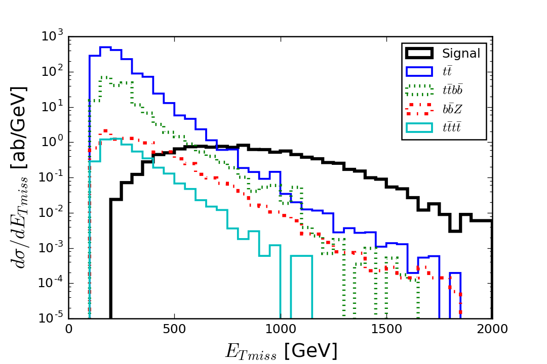
Even after these cuts, we must still contend with sizable backgrounds, as can be seen from Fig. 2 where we show the $\not\!\!{E_{T}}$ distribution from the $t\bar{t}$, $t\bar{t}b\bar{b}$, $b\bar{b}Z$, and $t\bar{t}t\bar{t}$ backgrounds, as well as from the gluino pair production for the benchmark point in Table 1. We see that the backgrounds fall more quickly with $\not\!\!{E_{T}}$ than the signal leading us to impose a $\not\!\!{E_{T}}$ cut,

$\not\!\!{E_{T}}$ Cut:

$$\not\!\!{E_{T}} > 750\ {\rm GeV}.$$ (5)

Figure 3: The number of $b$-tagged jets, using the Isajet parameterization of the $b$-tagging efficiency, after C1 cuts (4) and the requirement that $\not\!\!{E_{T}}>750$ GeV.

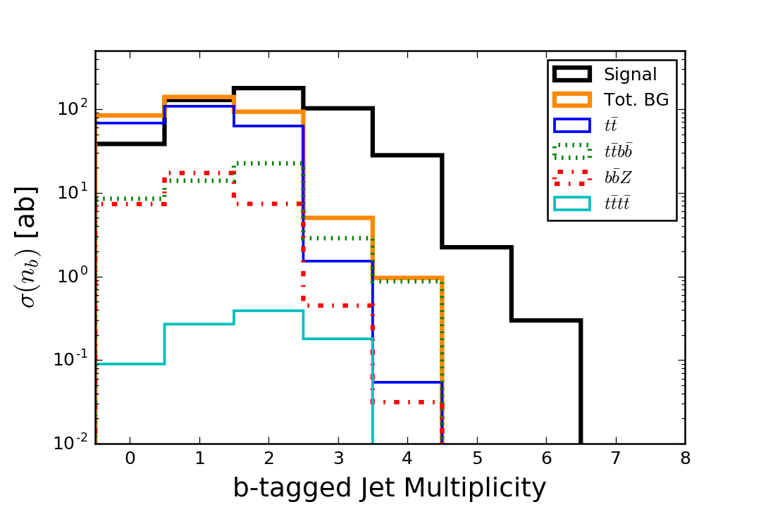
After this cut, we are left with comparable backgrounds from $t\bar{t}$ and $t\bar{t}b\bar{b}$ production with a somewhat smaller contribution from $b\bar{b}Z$ production. The $t\bar{t}t\bar{t}$ background rate is much smaller.

Once we have made the $\not\!\!{E_{T}}$ cut (5), we examine the distribution of the multiplicity of $b$-tagged jets, with the goal of further improving the signal to background ratio. This distribution is shown in Fig. 3. This figure suggests two roads to selection criteria that will leave a robust signal and negligible backgrounds. Obviously, we can require three $b$-tags, which decimates the backgrounds (especially $t\bar{t}$) at the cost of some signal. Our goal is to devise a strategy that will allow mass measurements even with integrated luminosities of 100-200 fb^-1 that will be available by the end of the 2018 LHC shutdown for which significant loss of event rate rapidly becomes a problem. With this in mind, we also examine the possibility that we can only require two $b$-tags. While this saves some signal, we clearly need to impose additional cuts to obtain a clean signal sample. We pursue both of these approaches: the larger cross section from the “$2b$” analysis will certainly be useful in early LHC running, but the greater reduction of backgrounds provided by the “$3b$” analysis would be expected to yield cleaner data samples at the high luminosity LHC.

Figure 4: The distribution of $\Delta\phi(\not\!\!{E_{T}},\ {\rm nearest~jet})$. Explicitly this quantity is the minimum angle between the $\not\!\!{E_{T}}$ vector and the transverse momentum of one of the leading four jets. This quantity is shown (left) after C1 cuts (4) with the requirement of two $b$-tagged jets and (right) after these cuts, and a cut of $\not\!\!{E_{T}}>750$ GeV.

To further clean up the $n_{b}\geq 2$ signal sample, we first note that that the bulk of the background comes from $t\bar{t}$ production. It is reasonable to expect that $t\bar{t}$ production leads to $\not\!\!{E_{T}}>750$ GeV only if a semi-leptonically decaying top is produced with a very high transverse momentum, with the daughter neutrino “thrown forward” in the top rest frame, while the other top decays hadronically (so the $\not\!\!{E_{T}}$ is not cancelled). In this case, the $b$-jet from the decay of the semi-leptonically decaying top would tend to be collimated with the neutrino; i.e., to the direction of $\not\!\!{E_{T}}$. We do not expect such a correlation in the signal since the heavy gluinos need not be particularly boosted to yield $\not\!\!{E_{T}}>750$ GeV. 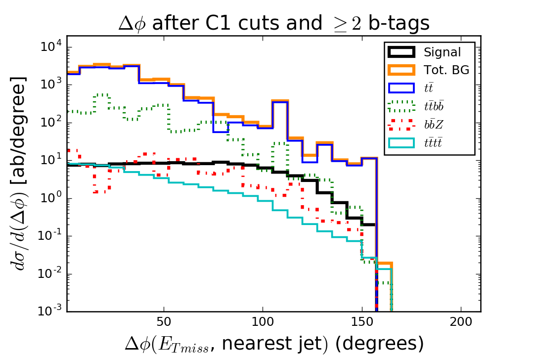This motivated us to examine the distribution of the minimum value of $\Delta\phi$, the angle between the transverse momenta of a jet and the $\not\!\!{E_{T}}$ vector, for each of the four leading jets. We show this distribution in Fig. 4, after the C1 and the two tagged $b$-jet cuts, both with (right frame) and without (left frame) the $\not\!\!{E_{T}}>750$ GeV cut. Without this hard $\not\!\!{E_{T}}$ cut, we see that the distribution of $\Delta\phi$ is very slowly falling for the $t\bar{t}$ background, and roughly flat for the signal as for the other backgrounds, until all the distributions cut-off at about $150^{\circ}$. The expected peaking of the $t\bar{t}$ background at low values of $\Delta\phi$ is, however, clearly visible in the right frame, while the signal is quite flat. The next-largest background from $t\bar{t}b\bar{b}$ also shows a similar peaking (for the same reason) at low $\Delta\phi$ values. We are thus led to impose the cut,

$\Delta\phi$ Cut:

$$\Delta\phi(\not\!\!{E_{T}},\rm{nearest~of~four~leading~jets}) > 30^{\circ},$$ (6)

which greatly diminishes the dominant backgrounds in the two tagged $b$-jet channel with only a very modest loss of signal. Indeed, because the signal-to-background ratio is so vastly improved with only a slight reduction of the signal, we have retained this cut in both our 2$b$ and $3b$ analyses.

Figure 5: The distribution of $\not\!\!{E_{T}}$ after C1 cuts (4), the $\not\!\!{E_{T}}>750$ cut (5), and the $\Delta\phi>30^{\circ}$ cut (6) with the additional requirement of (left) at least two $b$-tagged jets (right) at least three $b$-tagged jets. The background distribution represents the sum of the contributions from the $t\bar{t}$, $t\bar{t}b\bar{b}$, $b\bar{b}Z$, and $t\bar{t}t\bar{t}$ backgrounds.

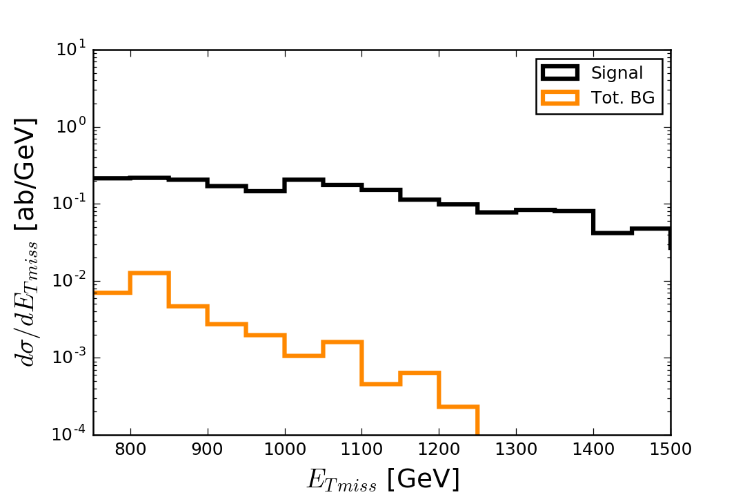
Having made this cut, we return to the $\not\!\!{E_{T}}$ distribution, to see whether further optimization might be possible. Toward this end, we show the distribution after the C1 cuts (4), the $\not\!\!{E_{T}}>750$ GeV cut (5), and the $\Delta\phi>30^{\circ}$ cut (6) in Fig. 5, requiring at least two $b$-tagged jets (left panel) or three $b$-tagged jets (right panel). We see that an additional cut on $\not\!\!{E_{T}}$ will be helpful in the $2b$ analysis, but not as helpful in the $3b$ analysis. Therefore, our final cut choices are:

$2b$ Analysis:

$${\rm C1~cuts},$$

$$n_{b} \geq 2,$$

$$\Delta\phi(\not\!\!{E_{T}},\rm{nearest~of~four~leading~jets}) > 30^{\circ},$$ (7)

$$\not\!\!{E_{T}} > 900\ {\rm GeV},$$

and

$3b$ Analysis:

$${\rm C1~cuts},$$

$$n_{b} \geq 3,$$

$$\Delta\phi(\not\!\!{E_{T}},\rm{nearest~of~four~leading~jets}) > 30^{\circ},$$ (8)

$$\not\!\!{E_{T}} > 750\ {\rm GeV},$$

The cross section including acceptance after each of the cuts, for the signal benchmark point, as well as for the sum of the $t\bar{t}$, $t\bar{t}b\bar{b}$, $b\bar{b}Z$ and $t\bar{t}t\bar{t}$ backgrounds, is given in Table 2, for both the $2b$ and the $3b$ analyses.

Cut	$2b$ Sig.	$2b$ BG	$3b$ Sig.	$3b$ BG
C1	$872$	$4.99\times 10^{5}$	$872$	$4.99\times 10^{5}$
$\not\!\!{E_{T}}>750$ GeV	$479$	$323$	$479$	$323$
$b$-tagging	$311$	$99.1$	$133$	$5.98$
$\Delta\phi>30^{\circ}$	$249$	$26.8$	$105$	$1.65$
Final $\not\!\!{E_{T}}$ cut	$167$	$5.02$	$105$	$1.65$

Table 2: Cross section times acceptance in attobarns (1000 ab$=$ 1 fb) after various cuts are applied. The “$b$-tagging” cut refers to the requirement of $\geq 2$ $b$-tagged jets in the $2b$ analysis and $\geq 3$ $b$-tagged jets in the $3b$ analysis. For the $2b$ analysis, the “final $\not\!\!{E_{T}}$ cut” refers to the additional requirement that $\not\!\!{E_{T}}>900$ GeV; there is no additional cut in the $3b$ analysis.

Figure 6: Transverse momenta of the leading jet and second-leading jet in $p_{T}$ (left) and for the third and fourth-leading jets (right) for signal and background events after $2b$ analysis cuts. The distribution of these quantities after $3b$ analysis cuts is similar.

4.1 Gluino Event Characteristics

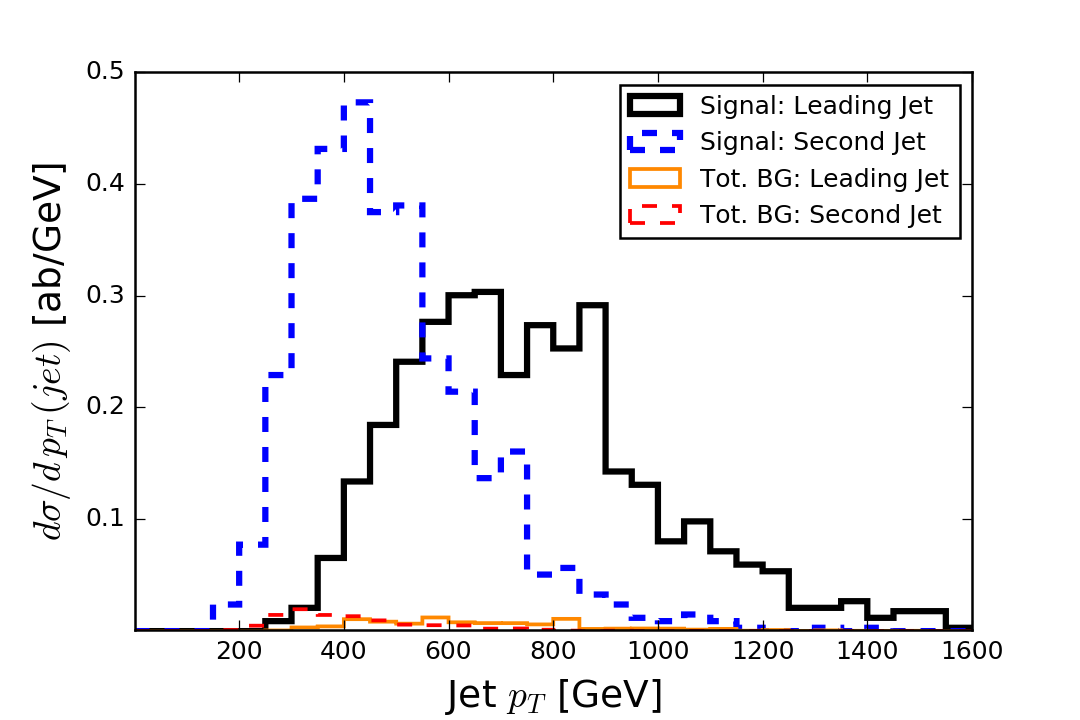
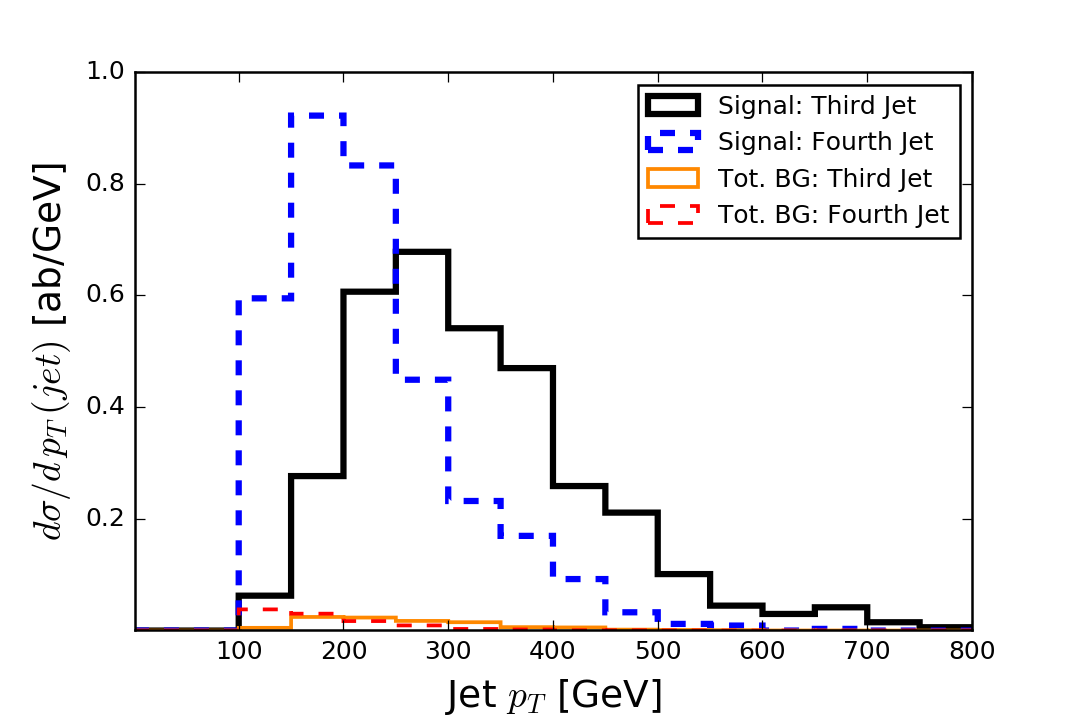
Now that we have finalized our analysis cuts, we display the characteristic features of gluino signal events satisfying our selection criteria for our natural SUSY benchmark point with $m_{\tilde{g}}\simeq 2$ TeV and $m_{\tilde{t}_{1}}\sim 1500$ TeV. Figure 6 shows the transverse energy distribution of the four hardest jets from the two-tagged $b$-jet signal as well as from the backgrounds, after the cut set (7). We see that the two hardest jets typically have $E_{T}\sim 700$ GeV and 400 GeV, respectively, while the third and fourth jet $E_{T}$ distributions peak just below 300 GeV and 200 GeV. The distributions for the signal with three tagged $b$-jets are very similar and not shown for brevity. While the actual peak positions in the distributions depend on the gluino and stop masses, the fact that the events contain four hard jets is rather generic. We also see that the SM background after these cuts is negligibly small, and that we do indeed have a pure sample of gluino events.

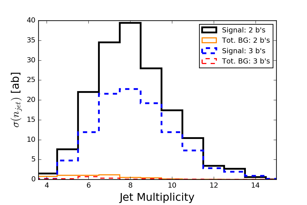
In Fig. 7, we show the jet multiplicity for the benchmark point signal and background events after our selection cuts for both the two tagged $b$-jet (solid) and the three-tagged $b$-jet (dashed) samples. Recall that jets are defined to be hadronic clusters with $E_{T}>50$ GeV. We see that the signal indeed has very high jet multiplicity relative to the background. Since the exact jet multiplicity may be sensitive to details of jet definition, and because our simulation of the background with very high jet multiplicity is less reliable due to the use of the shower approximation rather than exact matrix elements, we have not used jet multiplicity cuts to further enhance the signal over background. (Note: the sum of cross-sections above a minimum jet-multiplicity, as implemented in the C1 cuts, is not expected to depend much on the implementation of the jet multiplicity cut.)

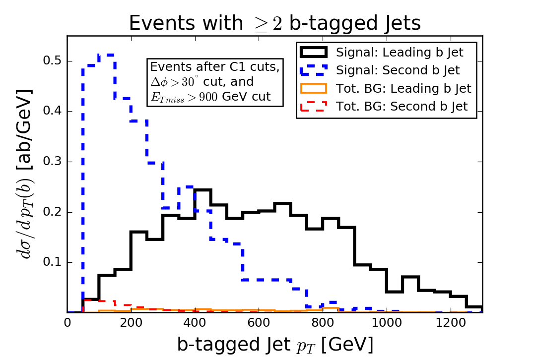
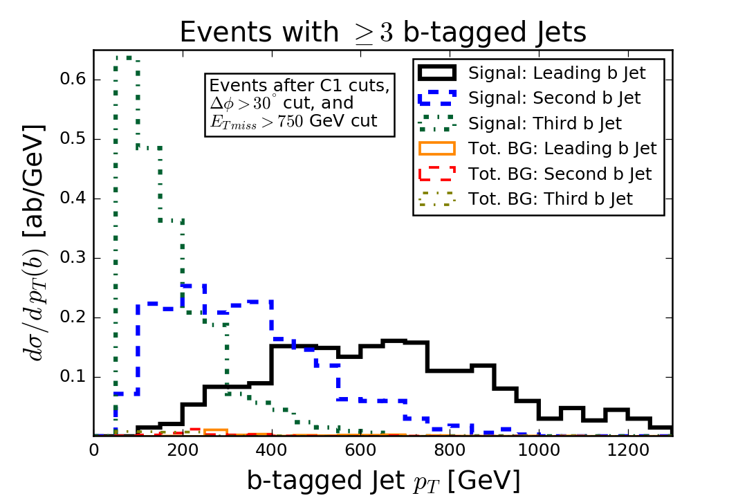
In Fig. 8 we show the transverse momentum of $b$-tagged jets in signal and background events satisfying the final cuts for $\geq 2$ tagged $b$-jet events (left frame) and for $\geq 3$ tagged $b$-jet events (right frame). We see that the hardest $b$-jet $E_{T}$ ranges up to $\sim 1$ TeV, while the second $b$-jet, for the most part, has $E_{T}\sim 100-600$ GeV. Again, we stress that the $b$-jet spectrum shape will be somewhat sensitive to the gluino-stop as well as stop-higgsino mass differences, but the hardness of the $b$-jets is quite general. We expect that the $b$-jets would remain hard (though the $E_{T}$ distributions would have different shapes) even in the case when the stop is heavier than the gluino, and the gluino instead dominantly decays via the three body modes, $\tilde{g}\rightarrow t\bar{t}\widetilde{Z}_{1,2}$ and $\tilde{g}\rightarrow tb\widetilde{W}_{1}$.

Figure 7: Jet multiplicity for signal and background events satisfying our $2b$ and $3b$ analysis cuts. Recall that we require jets to have $p_{T}>50$ GeV and $|\eta|<3.0$.

Figure 8: The distribution of the transverse momenta of the leading and second leading $b$-tagged jet after (left) the $2b$ analysis cuts and (right) the $3b$ analysis cuts.

Before turning to a discussion of our results for the mass reach and of the feasibility of the extraction of $m_{\tilde{g}}$ using the very pure sample of signal events, we address the sensitivity of our cross section calculations to the Isajet $b$-tagging efficiency and purity algorithm that we have used. This algorithm was based on early ATLAS studies  [43] of $WH$ and $t\bar{t}H$ processes where the transverse momentum of the $b$-jets is limited to several hundred GeV. More recently, the CMS Collaboration [46] has provided loose, medium and tight $b$-tagging algorithms with corresponding charm and light parton mis-tags whose validity extends out to a TeV. We show a comparison of the SUSY signal rate for our SUSY benchmark point for the sample with at least two/three tagged $b$-jets after the selection cuts (7)/(8) in Table 3. We illustrate results for the medium and tight algorithms in Ref. [46]. Also shown, in parenthesis are the corresponding signal-to-background ratios, after these cuts. We see that the cross sections for the Isajet parametrization of the $b$-tagging efficiency, as well as the corresponding values of $S/B$ lie between those obtained using the medium and tight algorithms in the recent CMS study. Although it is difficult to project just how well $b$-tagging will perform in the high luminosity environment, we are encouraged to see that our simple algorithm gives comparable answers to those obtained using the more recent tagging algorithms in Ref. [46] even though we have very hard $b$-jets in the signal.

	Isajet	CMS Medium	CMS Tight
$\geq 2$ tagged $b$ jets, $\not\!\!{E_{T}}>900$ GeV	167 (33)	207 (26)	121 (41)
$\geq 3$ tagged $b$ jets, $\not\!\!{E_{T}}>750$ GeV	105 (66)	182 (50)	61.1 (81)

Table 3: The LHC signal cross section in ab for our SUSY benchmark point for $\geq 2$ tagged $b$-jet events, and for $\geq 3$ tagged $b$-jet events after all the analysis cuts in (7) and (8), respectively. The numbers in parenthesis are the corresponding signal-to-background ratios. We show results for the Isajet parametrization of $b$-tagging efficiency as well as for the medium and tight $b$-tagging efficiencies in Ref. [46].

5 Results

In this section, we show that the pure sample of gluino events that we have obtained can be used to make projections for both the gluino mass reach as well as for the extraction of the gluino mass, along the RNS model line introduced at the start of Sec. 2. We consider several values of integrated luminosities at LHC14 ranging from 150 fb^-1 to the 3000 fb^-1 projected to be accumulated at the high luminosity LHC.

5.1 Gluino mass reach

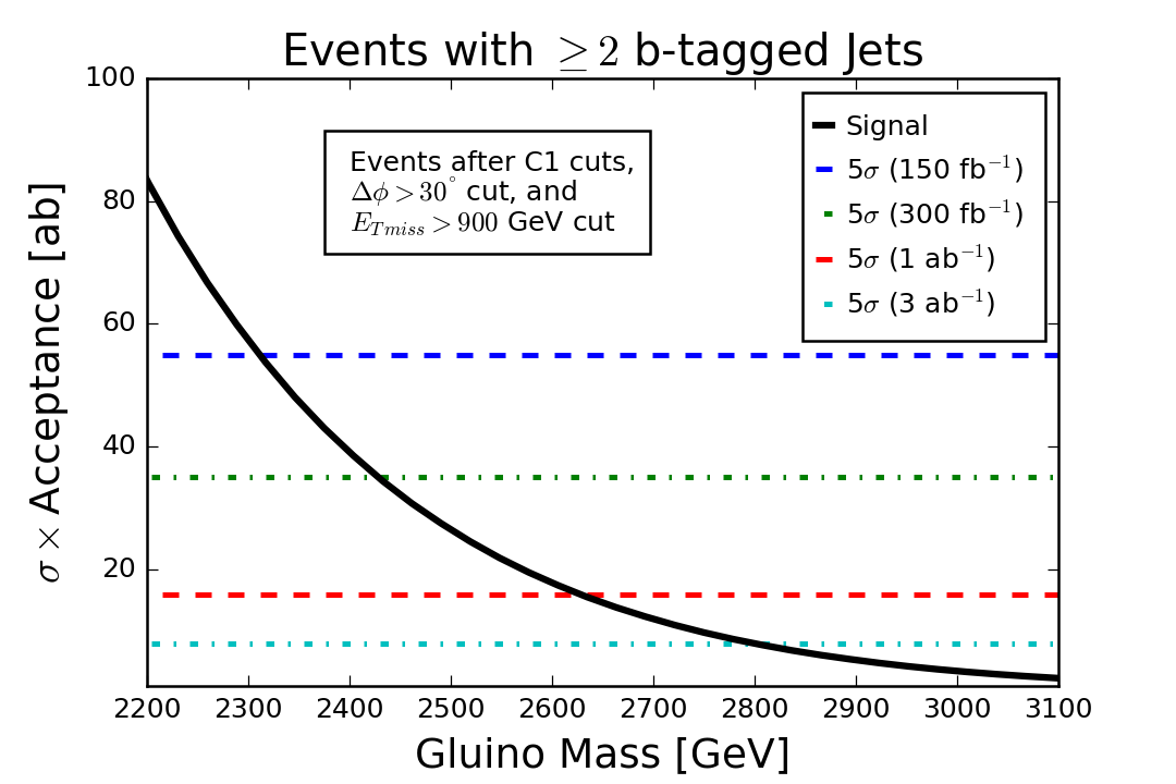
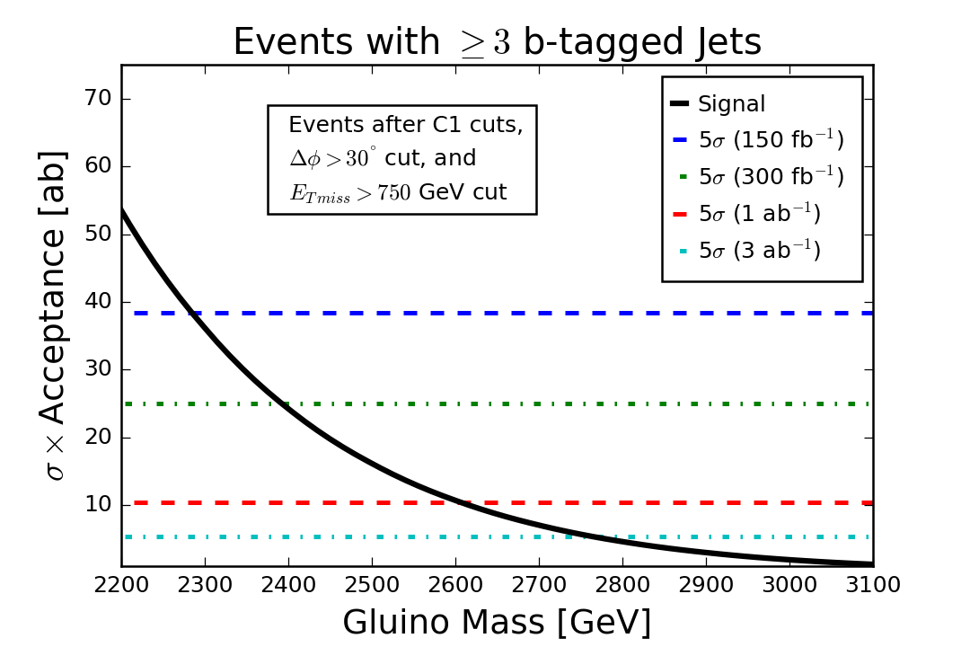
We begin by showing in Fig. 9 the gluino signal cross section after all analysis cuts via both the $\geq 2$ tagged $b$-jets (left frame) and the $\geq 3$ tagged $b$-jets (right frame) channels. The total SM backgrounds in these channels are 5.02 ab and 1.65 ab, respectively. The various horizontal lines show the minimum cross section for which a Poisson fluctuation of the expected background occurs with a Gaussian probability corresponding to $5\sigma$, for several values of integrated luminosities at LHC14, starting with 150 fb^-1 expected (per experiment) before the scheduled 2018 LHC shutdown, 300 fb^-1 the anticipated design integrated luminosity of LHC14, as well as 1 ab^-1 and 3 ab^-1 that are expected to be accumulated after the high luminosity upgrade of the LHC. We have checked that for an observable signal we always have a minimum of five events and a sizable signal-to-background ratio. (The lowest value for signal-to-background ratio we consider, i.e., the value at the maximum gluino mass for which we have $5\sigma$ discovery with at least five events is for 3000 fb^-1 in our $2b$ analysis, for which $S/B=1.6$.) We see from Fig. 9 that, with 150 fb^-1, LHC experiments would be probing $m_{\tilde{g}}$ values up to 2300 GeV (actually somewhat smaller since the machine energy is still 13 TeV) via the $2b$ analysis, with only a slightly smaller reach via the $3b$ analysis. Even for the decoupled squark scenario, we project a 3000 fb^-1 LHC14 $5\sigma$ gluino reach to $\sim 2400$ GeV; this will extend to about 2800 GeV in both the $2b$ and $3b$ channels at the HL-LHC. These projections are significantly greater than the corresponding reach from the mSUGRA model [54] because (1) the presence of hard $b$-jets in the signal serves as an additional handle to reduce SM backgrounds, especially those from $W,Z$+jet production processes [55], and (2) the larger $m_{\tilde{g}}-m_{\widetilde{Z}_{1}}$ mass gap expected from RNS leads to harder jets and harder $\not\!\!{E_{T}}$ as compared to mSUGRA. A further improvement in reach may of course be gained by combining ATLAS and CMS data sets.

Figure 9: The gluino signal cross section for the $\geq 2$ tagged $b$-jet (left) and the $\geq 3$ tagged $b$-jet channels (right) after all the analysis cuts described in the text. The horizontal lines show the minimum cross section for which the Poisson fluctuation of the corresponding SM background levels, 5.02 ab for $2b$ events and 1.65 ab for $3b$ events, occurs with a Gaussian probability corresponding to $5\sigma$ for integrated luminosities for several values of integrated luminosities at LHC14.

5.2 Gluino mass measurement

We now turn to the examination of whether the clean sample of gluino events that we have obtained allows us to extract the mass of the gluino. For decoupled first/second generation squarks, these events can only originate via gluino pair production. Assuming that the background is small, or can be reliably subtracted, the event rate is completely determined by $m_{\tilde{g}}$. A determination of this event rate after the analysis cuts in (7) or (8) should, in principle, yield a measure of the gluino mass.

Figure 10: Illustration of our method to extract the precision with which the gluino mass may be extracted at the LHC for the $2b$ sample (left frame) and the statistical precision that may be attained as a function of $m_{\tilde{g}}$ for integrated luminosities of 150 fb^-1, 300 fb^-1, 1 ab^-1 and 3 ab^-1 (right frame). The left frame shows a blow-up of the gluino signal cross section versus $m_{\tilde{g}}$ for the $\geq 2$ tagged $b$-jets after all the analysis cuts described in the text. Also shown are the “$1\sigma$” error bars for a determination of this cross section (where the $1\sigma$ statistical error on the observed number of signal events and a 15% uncertainty on the gluino production cross section have been combined in quadrature) for an integrated luminosity of 150 fb^-1 (blue) and 3 ab^-1 (red). The other lines show how we obtain the precision with which the gluino mass may be extracted for our benchmark gluino point for these two values of integrated luminosities. The bands in the right frame illustrate the statistical precision on the extracted value of $m_{\tilde{g}}$ that may be attained at the LHC for four different values of integrated luminosity. We terminate the shading at the $5\sigma$ discovery reach shown in Fig 9.

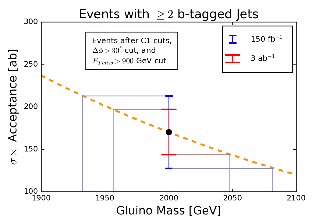
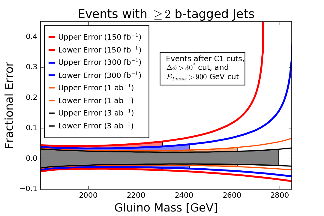
Our procedure for the extraction of the gluino mass (for our benchmark point) is illustrated in the left frame of Fig. 10, where we show a blow-up of the SUSY signal cross section versus $m_{\tilde{g}}$ for $\geq 2$ tagged $b$-jet events after all our analysis cuts. The signal cross section can be inferred from the observed number of events in the sample and subtracting the expected background. The error bar shown in the figure is obtained by combining in quadrature the $1\sigma$ statistical error on the cross section based on the expected total number of (signal plus background) events expected in the sample, with a 15% theoretical error on the gluino production cross section. This error bar is used to project “the $1\sigma$” uncertainty in the measurement of $m_{\tilde{g}}$. From the figure, $m_{\tilde{g}}=2000^{+80}_{-70}$ GeV with 150 fb^-1, and $m_{\tilde{g}}=(2000^{+50}_{-45})$ GeV with 3 ab^-1. The right frame of Fig. 10 shows the precision with which the gluino mass may be extracted via the clean events in the $\geq 2$ tagged $b$-jets channel versus the gluino mass for four different values of integrated luminosity ranging from 150 fb^-1 to 3 ab^-1. The shading on the various bands extends out to the $5\sigma$ reach projection in Fig. 9. We see that gluino mass extraction with a sub-ten percent precision is possible with even 150 fb^-1 of integrated luminosity if gluinos are lighter than 2.5 TeV and cascade decay via stops into light higgsinos as in the RNS framework. It should be noted though that the $5\sigma$ reach of the LHC extends to just $\sim 2.3$ TeV so that the determination, $m_{\tilde{g}}=2.5$ TeV would be a mass measurement for a discovery with a significance smaller than the customary $5\sigma$. At the high luminosity LHC, the gluino mass may be extracted with a statistical precision better than 2.5-4% (depending on their mass) all the way up to $m_{\tilde{g}}\sim 2.8$ TeV, i.e, if gluinos are within the $5\sigma$ discovery range of the HL-LHC! Gluino mass determination would also be possible for the range of gluino masses for which the discovery significance was smaller than $5\sigma$.

Figure 11: The same as Fig. 10, but for the clean SUSY sample with $\geq 3$ tagged $b$-jets.

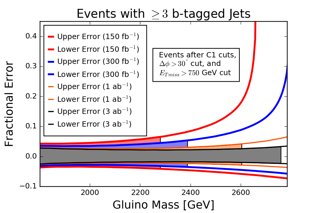
Prospects for gluino mass measurement via the $\geq 3$ tagged $b$-jet sample are shown in Fig. 11. We see that the statistical precision on the mass measurement that may be attained is somewhat worse than that via the $\geq 2b$ channel shown in Fig. 10, though not qualitatively different except at the high mass end. The difference is, of course, due to the lower event rate in this channel.

Before proceeding further, we point out that in order to extract the gluino mass, we have assumed that our estimate of the background is indeed reliable. Since the expected background has to be subtracted from the observed event rate to obtain the signal cross section, and via this the value of $m_{\tilde{g}}$, any error in the estimation of the expected background will result in a systematic shift in the extracted gluino mass. For instance, an over-estimation of the background expectation compared to its true value, will result in too small a signal and a corresponding overestimate of the mass of the gluino. We expect that by the time a precise mass measurement becomes feasible, it will be possible to extract the SM background to a good precision by extrapolating the backgrounds normalized in the “background region” (that are expected to have low signal contamination) to the “signal region” using the accumulated data.

Figure 12: The systematic bias, discussed in the text, in the measurement of the gluino mass resulting from a mis-estimate of the SM background by a factor of 2 in either direction. The solid lines are for the signal in the $2b$ channel while the dashed lines are for the signal in the $3b$ channel.

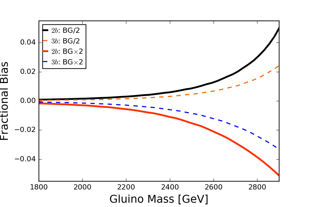
We show in Fig. 12 the systematic bias on the gluino mass that could result because the background estimate differs from the true value by a factor of 2. We see that this (asymmetric) systematic bias is below 2% for $m_{\tilde{g}}\stackrel{{\scriptstyle<}}{{\sim}}2.6$ TeV, but becomes as large as 4% for the largest masses for which there is a 5$\sigma$ signal at the high luminosity LHC in the two tagged $b$-jets sample. This bias is smaller for the three tagged $b$-jets sample because the corresponding background is smaller.

Our conclusions for the precision with which LHC measurements might extract the gluino mass are very striking, and we should temper these with some cautionary remarks. The most important thing is that any extraction of the mass from the absolute event rate assumes an excellent understanding of the detector in today’s environment as well as in the high luminosity environment of future experiments. While we are well aware that our theorists’ simulation does not include many important effects, e.g., particle detection efficiencies, jet energy scales, full understanding of $b$-tagging efficiencies particularly for very high $E_{T}$ $b$-jets, to name a few, we are optimistic that these will all be very well understood (given that there will be a lot of data) by the time gluino mass measurements become feasible. The fact that our proposal relies on an inclusive cross section with $\geq 4$ jets (of which 2 or 3 are $b$-jets) and does not entail very high jet multiplicities suggests that our procedure should be relatively robust. An excellent understanding of the $\not\!\!{E_{T}}$ tail from SM sources, as well as of the tagging efficiency (and associated purity) for very high $E_{T}$ $b$-jets are crucial elements for this analysis.

6 Summary

In this paper, we have re-examined LHC signals from the pair production of gluinos assuming gluinos decay via $\tilde{g}\rightarrow t\tilde{t}_{1}$, followed by stop decays, $\tilde{t}_{1}\rightarrow b\widetilde{W}_{1},t\widetilde{Z}_{1,2}$, to higgsinos, where the visible decay products of the higgsinos are very soft. This is the dominant gluino decay chain expected within the radiatively-driven natural SUSY framework that we have suggested for phenomenological analysis of simple natural SUSY GUT models. For our analysis, we have used the RNS model line detailed in Sec. 2 with higgsino masses $\sim 150$ GeV. The gluino signal then consists of events with $\geq 4$ hard jets, two or three of which are tagged as $b$-jets together with very large $\not\!\!{E_{T}}$. We expect that our results are only weakly sensitive to our choice of higgsino mass as long as the electroweak fine-tuning parameter $\Delta_{\rm EW}\stackrel{{\scriptstyle<}}{{\sim}}30$.

The new features that we have focussed on in this analysis are the very large data sets (300-3000 fb^-1) that are expected to be available at the LHC and its high luminosity upgrade and the capability for tagging very hard $b$-jets with $E_{T}$ up to a TeV and beyond. We have identified a set of very stringent cuts, detailed in (7) and (8), that allows us to isolate the gluino signal from SM backgrounds: our procedure yields a signal to background $>30$ ($>60$) in the two (three) tagged $b$-jets channel for $m_{\tilde{g}}=2$ TeV, and $>4$ ($>10$) for $m_{\tilde{g}}=2.6$ TeV. Even for decoupled squarks, these relatively pure data samples extend the gluino discovery reach in the RNS framework to 2.4 TeV for an integrated luminosity of 300 fb^-1 expected by end of the current LHC run, and to 2.8 TeV with 3000 fb^-1 anticipated after the luminosity upgrade of the LHC. These may be compared to projections [54] for the gluino reach of 1.8 TeV (2.3 TeV) for 300 fb^-1 (3000 fb^-1) within the mSUGRA/CMSSM framework. We attribute the difference to, (1) the presence of $b$-jets in the signal which serve to essentially eliminate SM backgrounds from $V$+jet production, and also reduce those from other sources and (2) the comparatively harder jet $E_{T}$ and $\not\!\!{E_{T}}$ spectrum associated with RNS models.

The separation of a relatively clean gluino sample also allows a determination of the gluino mass based on the signal event rate rather than kinematic properties of the event. Although the determination of the mass from the event rate hinges upon being able to predict the absolute normalization of the expected signal after cuts, and so requires an excellent understanding of the detector, we are optimistic that LHC experimenters will be able to use the available data to be able to reliably determine acceptances and efficiencies in the signal region by the time these measurements become feasible. We project that with 300 fb^-1 of integrated luminosity, experiments at LHC14 should be able to measure $m_{\tilde{g}}$ with a $1\sigma$ statistical error of $<4.5$% for $m_{\tilde{g}}=2.4$ TeV, i.e., all the way up to its $5\sigma$ discovery limit. At the high luminosity LHC, the projected precision for a gluino mass measurement ranges between about 2.5% for $m_{\tilde{g}}=2$ TeV to about 4% near its $5\sigma$ discovery limit of 2.8 TeV in the $\geq 2$ tagged $b$-jet channels. Comparable precision is obtained also via the $\geq 3$ tagged $b$ channel. In this connection, we should also keep in mind that a factor of two uncertainty in the projected background will result in a small (but not negligible) systematic uncertainty ranging between $<1$% for $m_{\tilde{g}}<2500$ GeV to about 3% for $m_{\tilde{g}}=2800$ GeV in the extraction of $m_{\tilde{g}}$ via the $\geq 2$ tagged $b$ channel and smaller than this for the $\geq 3$ tagged $b$ channel.

An observation of a SUSY signal in both $2b$ and $3b$ channels, and the extraction of a common value of $m_{\tilde{g}}$ would certainly be strong evidence for a discovery of a new particle. If these signals are accompanied by other signals such as the same-sign diboson signal and/or monojet events with soft opposite sign dileptons, the case for the discovery of radiatively-driven natural SUSY would be very strong. In this case, depending on the gluino mass, there may also be signals in trilepton and even four lepton plus jets plus $\not\!\!{E_{T}}$ channels [25].

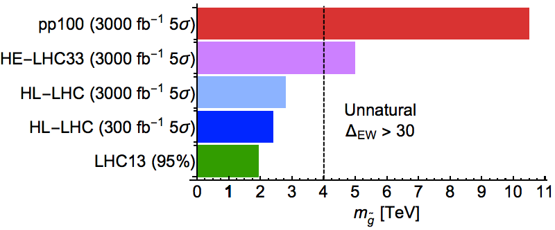
In Fig. 13 we compare the approximate reach for various present and future hadron collider options for gluino pair production. The region to the right of the dashed line yields large electroweak fine-tuning and is considered unnatural. The green bar shows the present LHC 95% CL limit on $m_{\tilde{g}}$ as derived in several simplified models which should be applicable to the present RNS case. The dark and light blue bars show our projected LHC14 300 and 3000 fb^-1 $5\sigma$ reaches for RNS. These cover only a portion of natural SUSY parameter space. The lavendar bar shows the reach of HE-LHC with $\sqrt{s}=33$ TeV as abstracted from Ref. [56] where it is assumed that the gluino directly decays to a light LSP via $\tilde{g}\rightarrow q\bar{q}\widetilde{Z}_{1}$ (presumably with no enhancement of decays to third generation quarks). The $5\sigma$ HE-LHC for 3000 fb^-1 extends to $m_{\tilde{g}}\sim 5$ TeV and thus covers all of natural SUSY parameter space. The red bar shows the corresponding gluino reach of a 100 TeV $pp$ collider at $5\sigma$ and 3000 fb^-1, as taken also from Ref. [56]. Here, the reach extends just beyond $m_{\tilde{g}}\sim 10$ TeV. It probes only more deeply into unnatural SUSY parameter space beyond the complete coverage of the gluino offered by HE-LHC, but does offer the possibility of a squark discovery.

Figure 13: The approximate reach for various present and future hadron collider options for gluino pair production. The region to the right of the dashed line yields large electroweak fine-tuning and is considered unnatural.

In summary, in models such as RNS where gluinos dominantly decay via $\tilde{g}\rightarrow t\tilde{t}_{1}$, and the stops decay to light higgsinos via $\tilde{t}_{1}\rightarrow\widetilde{W}_{1}b$, $\widetilde{Z}_{1,2}t$, signals from gluino pair production should be observable at the $5\sigma$ level out to $m_{\tilde{g}}<2.4\ (2.8)$ TeV for an integrated luminosity of 300 fb^-1 (3000 fb^-1) in the $\geq 4$-jet sample with very hard $\not\!\!{E_{T}}$ and two or three tagged $b$-jets. The clean sample of gluino events that we obtain should also allow a measurement of $m_{\tilde{g}}$ with a statistical precision ranging from 2.5-4% depending on the gluino mass and the integrated luminosity, along with a smaller but non-negligible systematic uncertainty of 1-3% mentioned in the previous paragraph. The precision of gluino mass extraction should be even greater using the combined ATLAS/CMS data set.

References

- [1] E. Witten, Nucl. Phys. B 188, 513 (1981); R. K. Kaul, Phys. Lett. B 109, 19 (1982).
- [2] S. Dimopoulos, S. Raby and F. Wilczek, Phys. Rev. D 24 (1981) 1681; U. Amaldi, W. de Boer and H. Furstenau, Phys. Lett. B 260, 447 (1991); J. R. Ellis, S. Kelley and D. V. Nanopoulos, Phys. Lett. B 260 (1991) 131; P. Langacker and M. x. Luo, Phys. Rev. D 44 (1991) 817.
- [3] L. E. Ibañez and G. G. Ross, Phys. Lett. B110, 215 (1982); K. Inoue et al. Prog. Theor. Phys. 68, 927 (1982) and 71, 413 (1984); L. Ibañez, Phys. Lett. B118, 73 (1982); H. P. Nilles, M. Srednicki and D. Wyler, Phys. Lett. B 120 (1983) 346; J. Ellis, J. Hagelin, D. Nanopoulos and M. Tamvakis, Phys. Lett. B125, 275 (1983); L. Alvarez-Gaumé. J. Polchinski and M. Wise, Nucl. Phys. B221, 495 (1983); B. A. Ovrut and S. Raby, Phys. Lett. B 130 (1983) 277; for a review, see L. E. Ibanez and G. G. Ross, Comptes Rendus Physique 8 (2007) 1013.
- [4] G. Aad et al. [ATLAS Collaboration], Phys. Lett. B 716 (2012) 1; S. Chatrchyan et al. [CMS Collaboration], Phys. Lett. B 716 (2012) 30.
- [5] H. E. Haber and R. Hempfling, Phys. Rev. Lett. 66 (1991) 1815; J. R. Ellis, G. Ridolfi and F. Zwirner, Phys. Lett. B 257 (1991) 83; Y. Okada, M. Yamaguchi and T. Yanagida, Prog. Theor. Phys. 85 (1991) 1; For a review, see e.g. M. S. Carena and H. E. Haber, Prog. Part. Nucl. Phys. 50 (2003) 63 [hep-ph/0208209].
- [6] G. Aad et al. [ATLAS Collaboration], JHEP 1409 (2014) 176; G. Aad et al. [ATLAS Collaboration], JHEP 1504 (2015) 116; CMS Collaboration [CMS Collaboration], CMS-PAS-SUS-14-011.
- [7] The ATLAS collaboration, ATLAS-CONF-2015-067.
- [8] W. Adam, Plenary talk presented at the 38th International Conference on High Energy Physics, Chicago, USA (Aug. 2016).
- [9] R. Barbieri and G. F. Giudice, Nucl. Phys. B 306, 63 (1988); this measure was introduced in J. R. Ellis, K. Enqvist, D. V. Nanopoulos and F. Zwirner, Mod. Phys. Lett. A 1, 57 (1986).
- [10] H. Baer, V. Barger and M. Savoy, Phys. Rev. D 93 (2016) 3, 035016.
- [11] G. Aad et al. [ATLAS Collaboration], JHEP 1411 (2014) 118; S. Chatrchyan et al. [CMS Collaboration], Eur. Phys. J. C 73 (2013) no.12, 2677.
- [12] S. Dimopoulos and G. F. Giudice, Phys. Lett. B 357 (1995) 573.
- [13] M. Papucci, J. T. Ruderman and A. Weiler, JHEP 1209 (2012) 035; C. Brust, A. Katz, S. Lawrence and R. Sundrum, JHEP 1203 (2012) 103.
- [14] J. Lykken and M. Spiropulu, Sci. Am. 310N5 (2014) 36; see also, A. Strumia, JHEP 1104 (2011) 073; N. Craig, arXiv:1309.0528; M. Dine, Ann. Rev. Nucl. Part. Phys. 65 (2015) 43.
- [15] H. Baer, V. Barger, P. Huang, A. Mustafayev and X. Tata, Phys. Rev. Lett. 109 (2012) 161802.
- [16] H. Baer, V. Barger, P. Huang, D. Mickelson, A. Mustafayev and X. Tata, Phys. Rev. D 87 (2013) 11, 115028.
- [17] H. Baer, V. Barger and D. Mickelson, Phys. Rev. D 88, 095013 (2013).
- [18] A. Mustafayev and X. Tata, Indian J. Phys. 88 (2014) 991.
- [19] H. Baer, V. Barger, D. Mickelson and M. Padeffke-Kirkland, Phys. Rev. D 89, 115019 (2014).
- [20] H. Baer, V. Barger and M. Savoy, Phys. Scripta 90 (2015) 068003 doi:10.1088/0031-8949/90/6/068003.
- [21] C. Brust, A. Katz, S. Lawrence and R. Sundrum, JHEP 1203 (2012) 103.
- [22] H. Baer, V. Barger and M. Savoy, Phys. Rev. D 93 (2016) no.7, 075001.
- [23] H. Baer, V. Barger and A. Mustafayev, Phys. Rev. D 85 (2012) 075010.
- [24] H. Baer, X. Tata and J. Woodside, Phys. Rev. D 42 (1990) 1568; H. Baer, C. h. Chen, M. Drees, F. Paige and X. Tata, Phys. Rev. D 58 (1998) 075008.
- [25] H. Baer, V. Barger, P. Huang, D. Mickelson, A. Mustafayev, W. Sreethawong and X. Tata, JHEP 1312 (2013) 013.
- [26] B. Altunkaynak, H. Baer, V. Barger and P. Huang, Phys. Rev. D 92 (2015) no.3, 035015.
- [27] H. Baer, V. Barger, P. Huang, D. Mickelson, A. Mustafayev, W. Sreethawong and X. Tata, Phys. Rev. Lett. 110 (2013) no.15, 151801.
- [28] Z. Han, G. D. Kribs, A. Martin and A. Menon, Phys. Rev. D 89 (2014) no.7, 075007; H. Baer, A. Mustafayev and X. Tata, Phys. Rev. D 90 (2014) no.11, 115007; C. Han, D. Kim, S. Munir and M. Park, JHEP 1504 (2015) 132.
- [29] H. Baer, V. Barger, M. Savoy and X. Tata, Phys. Rev. D 94 (2016) 035025.
- [30] H. Baer, V. Barger, D. Mickelson, A. Mustafayev and X. Tata, JHEP 1406 (2014) 172.
- [31] H. Baer, M. Berggren, K. Fujii, S. L. Lehtinen, J. List, T. Tanabe and J. Yan, arXiv:1611.02846 [hep-ph].
- [32] H. Baer, V. Barger, M. Padeffke-Kirkland and X. Tata, Phys. Rev. D 89 (2014) 037701.
- [33] H. Baer, V. Barger, G. Shaughnessy, H. Summy and L. t. Wang, Phys. Rev. D 75 (2007) 095010.
- [34] W. S. Cho, K. Choi, Y. G. Kim and C. B. Park, Phys. Rev. Lett. 100 (2008) 171801; M. M. Nojiri, Y. Shimizu, S. Okada and K. Kawagoe, JHEP 0806 (2008) 035; K. Agashe, R. Franceschini and D. Kim, JHEP 1411 (2014) 059; M. Burns, K. Kong, K. T. Matchev and M. Park, JHEP 0903 (2009) 143; W. S. Cho et al. JHEP 1408 (2014) 070.
- [35] D. Matalliotakis and H. P. Nilles, Nucl. Phys. B 435 (1995) 115; P. Nath and R. L. Arnowitt, Phys. Rev. D 56 (1997) 2820; J. Ellis, K. Olive and Y. Santoso, Phys. Lett. B539 (2002) 107; J. Ellis, T. Falk, K. Olive and Y. Santoso, Nucl. Phys. B652 (2003) 259; H. Baer, A. Mustafayev, S. Profumo, A. Belyaev and X. Tata, JHEP0507 (2005) 065.
- [36] ISAJET, by H. Baer, F. Paige, S. Protopopescu and X. Tata, hep-ph/0312045.
- [37] W. Beenakker, R. Hopker, M. Spira and P. M. Zerwas, Nucl. Phys. B 492, 51 (1997) doi:10.1016/S0550-3213(97)80027-2 [hep-ph/9610490].
- [38] W. Beenakker, S. Brensing, M. n. Kramer, A. Kulesza, E. Laenen, L. Motyka and I. Niessen, Int. J. Mod. Phys. A 26, 2637 (2011) doi:10.1142/S0217751X11053560 [arXiv:1105.1110 [hep-ph]].
- [39] K. J. Bae, H. Baer and E. J. Chun, Phys. Rev. D 89 (2014) no.3, 031701; K. J. Bae, H. Baer and E. J. Chun, JCAP 1312 (2013) 028; K. J. Bae, H. Baer, A. Lessa and H. Serce, JCAP 1410 (2014) no.10, 082.
- [40] J. Alwall, M. Herquet, F. Maltoni, O. Mattelaer and T. Stelzer, JHEP 1106 (2011) 128.
- [41] T. Sjostrand, S. Mrenna and P. Z. Skands, Comput. Phys. Commun. 178 (2008) 852.
- [42] J. de Favereau et al. [DELPHES 3 Collaboration], JHEP 1402 (2014) 057.
- [43] S. Corréad, V. Kostioukine, J. Levêque, A. Rozanov, J. B. de Vivie, ATLAS Note, ATLAS-PHYS-2004-006, and V. Kostioukine, ATLAS Note, ATLAS-PHYS-2003-033.
- [44] M. Cacciari, G. P. Salam and G. Soyez, JHEP 0804, 063 (2008) doi:10.1088/1126-6708/2008/04/063 [arXiv:0802.1189 [hep-ph]].
- [45] M. Cacciari, G. P. Salam and G. Soyez, Eur. Phys. J. C 72, 1896 (2012) doi:10.1140/epjc/s10052-012-1896-2 [arXiv:1111.6097 [hep-ph]].
- [46] CMS Collaboration [CMS Collaboration], CMS-PAS-BTV-15-001.
- [47] M. Cacciari and G. P. Salam, Phys. Lett. B 659, 119 (2008) doi:10.1016/j.physletb.2007.09.077 [arXiv:0707.1378 [hep-ph]].
- [48] M. Czakon, P. Fiedler and A. Mitov, Phys. Rev. Lett. 110, 252004 (2013) doi:10.1103/PhysRevLett.110.252004 [arXiv:1303.6254 [hep-ph]].
- [49] A. Bredenstein, A. Denner, S. Dittmaier and S. Pozzorini, JHEP 1003, 021 (2010) doi:10.1007/JHEP03(2010)021 [arXiv:1001.4006 [hep-ph]].
- [50] A. Bredenstein, A. Denner, S. Dittmaier and S. Pozzorini, Phys. Rev. Lett. 103 (2009) 012002.
- [51] F. Febres Cordero, L. Reina and D. Wackeroth, Phys. Rev. D 80, 034015 (2009) doi:10.1103/PhysRevD.80.034015 [arXiv:0906.1923 [hep-ph]].
- [52] G. Bevilacqua and M. Worek, JHEP 1207, 111 (2012) doi:10.1007/JHEP07(2012)111 [arXiv:1206.3064 [hep-ph]].
- [53] I. Hinchliffe, F. E. Paige, M. D. Shapiro, J. Soderqvist and W. Yao, Phys. Rev. D 55 (1997) 5520; H. Bachacou, I. Hinchliffe and F. E. Paige, Phys. Rev. D 62 (2000) 015009.
- [54] H. Baer, V. Barger, A. Lessa, X. Tata, Phys. Rev. D 86 (2012) 117701.
- [55] U. Chattopadhyay, A. Datta, A. Datta, A. Datta, and D. P. Roy, Phys. Lett. B 493 (2000) 127; J. K. Mizukoshi, P. Mercadante and X. Tata , Phys. Rev. D 72 (2005) 035009; R. Kadala, J. K. Mizukoshi, P. Mercadante and X. Tata, Eur. Phys. J C 56 (2008) 511.
- [56] Y. Gershtein et al., arXiv:1311.0299 [hep-ex].
- [57] A. Fowlie, arXiv:1510.07319 [hep-ph].