A line search algorithm for Wind field adjustment with incomplete data and RBF approximation

Daniel A. Cervantes Instituto de Matemáticas
UNAM
CDMX.
dcchivela@ciencias.unam.mx
Pedro González Casanova Instituto de Matemáticas
UNAM
CDMX.
casanova@matem.unam.mx
Christian Gout INSA Rouen
France.
christian.gout@insa-rouen.fr
 and  Miguel Ángel Moreles Centro de Investigaciones en Matemáticas
Guanajuato México
moreles@cimat.mx
Abstract.

The problem of concern in this work is the construction of free divergence fields given scattered horizontal components. As customary, the problem is formulated as a PDE constrained least squares problem. The novelty of our approach is to construct the so called adjusted field, as the unique solution along an appropriately chosen descent direction. The latter is obtained by the adjoint equation technique. It is shown that the classical adjusted field of Sasaki’s is a particular case. On choosing descent directions, the underlying mass consistent model leads to the solution of an elliptic problem which is solved by means of a Radial Basis Functions method. Finally some numerical results for wind field adjustment are presented.

1991 Mathematics Subject Classification:
2000 Math Subject Classification: 34K30, 35K57, 35Q80, 92D25
*Corresponding author

1. Introduction

The problem of recovering atmospheric wind fields from prescribed horizontal data is of great interest in meteorological applications. In practice the vertical component is unavailable. Consequently, measured data is complemented with mass consistency to pose a variational problem for approximation. This approach dates back to Sasaki [4]. Literature on the subject is vast, a timely review is presented in Ratto et al [6] .

The numerical approximation of the variational problem requires the solution of Poisson boundary value problems. Numerical approximations of the solutions can be obtained conventionally using the Finite Element Method, Finite Volume Method, Finite Differences, etc. In these methods mesh managing is computationally expensive. For the wind field adjustment problem, a case can be made for a mesh-free approach in terms of Radial Basis Functions (RBF). See Pepper, Rasmussen & Fyda [3], and Cervantes et al [5].

In the context of RBF, the problem of wind field recovery has been also considered as a smoothing problem. Mass consistency is introduced by penalizing with the norm of the divergence of the vector field. For the case of polyharmonic splines, Benbourhim and Bouhamidi [1], developed a smoothing algorithm for a given set of prescribed data in two and three dimensions. A full convergence analysis is provided. These RBF techniques can be traced back to Duchon’s works on thin plate splines [2].

The objective here, is to build on these methodologies and contribute on two unresolved issues. The wind field adjustment problem is posed on a bounded domain and boundary conditions are to be imposed, for instance the topography of the surface. The smoothing approach considers for approximation a linear combination of polyharmonic splines, imposing boundary conditions is not straightforward. In the Sasaki’s approach, boundary conditions are imposed somewhat heuristically. Also, given that only the first two components of the field are known, an initial guess of the third component is required in this approach. Common practice is unsatisfactory: since measurements of the vertical velocity component are seldom available, the initial vertical is usually set to zero. Ratto et al [6].

Consequently, in this work the problem is dealt with the data available in practice. Namely, the least squares functional to be introduced only involves the two known components. Minimization is carried out on descent directions, boundary conditions arise naturally and can be imposed on physical grounds. A RBF method is used for approximation. Finally, a proper abstract setting for analysis and numerics is provided.

This article is organized as follows.

In Section 2 the Hilbert function spaces are introduced, and the variational problem is formulated. From basic results form minimization of convex functionals on Hilbert spaces, existence of minima is proven. The construction of the adjusted mass consistent field is the content of Section 3. Also, the Sasaki solution is derived as a particular case. In Section 4 we discuss boundary conditions for the Poisson problems arising form the line search algorithm, and the RBF discretisation. Numerical results are presented in Section 5, noteworthy the vortex field in Benbourhim and Bouhamidi. Conclusions and comments on future research close this exposition.

2. Reconstruction of mass consistent vector fields with unknown vertical component

2.1. Problem Formulation

Assume the first two components of a 3D3𝐷3D vector field are known at N𝑁N non uniform points. Namely 𝐔i0=(u1(𝐱i),u2(𝐱i)),i=1,2,,Nformulae-sequencesubscriptsuperscript𝐔0𝑖subscript𝑢1subscript𝐱𝑖subscript𝑢2subscript𝐱𝑖𝑖12𝑁\mathbf{U}^{0}_{i}=(u_{1}(\mathbf{x}_{i}),u_{2}(\mathbf{x}_{i})),\ i=1,2,\ldots,N, for 𝐱iΩ3subscript𝐱𝑖Ωsuperscript3\mathbf{x}_{i}\in\Omega\subset\mathbb{R}^{3}.


Problem. Construct a flow field 𝐮(𝐱)=(u1(𝐱),u2(𝐱),u3(𝐱))𝐮𝐱subscript𝑢1𝐱subscript𝑢2𝐱subscript𝑢3𝐱\mathbf{u}(\mathbf{x})=(u_{1}(\mathbf{x}),u_{2}(\mathbf{x}),u_{3}(\mathbf{x})) in the entire domain ΩΩ\Omega, assuming that the set of discrete field values are known and that the approximant satisfies the continuity equation

𝐮=0.𝐮0\nabla\cdot\mathbf{u}=0.

The classical approach is as follows:

  1. (1)

    Initialization. From 𝐔i0,i=1,2,,Nformulae-sequencesubscriptsuperscript𝐔0𝑖𝑖12𝑁\mathbf{U}^{0}_{i},\ i=1,2,\ldots,N, determine an initial field 𝐮0(x)superscript𝐮0𝑥\mathbf{u}^{0}(x) entirely in ΩΩ\Omega.

  2. (2)

    Correction. By means of a minimization procedure, adjust 𝐮0superscript𝐮0\mathbf{u}^{0} to a reconstructed field satisfying mass conservation.

Our focus is on (2).


Function spaces

Let Ω3Ωsuperscript3\Omega\subset\mathbb{R}^{3} with boundary ΓΓ\Gamma. We assume that ΩΩ\Omega is a Lipschitz domain. We shall be concerned with nlimit-from𝑛n-dimensional vector functions. As customary we denote

𝐗=Xn,𝐗superscript𝑋𝑛\mathbf{X}=X^{n},

e.g.,

𝐋2(Ω)=(L2(Ω)))n\mathbf{L}^{2}(\Omega)=\left(L^{2}(\Omega))\right)^{n}

Let 𝐄(Ω)E(Ω)n𝐄Ω𝐸superscriptΩ𝑛\mathbf{E}(\Omega)\equiv E(\Omega)^{n} be the space

𝐄(Ω)={𝐮𝐋2(Ω):𝐮L2(Ω)}𝐄Ωconditional-set𝐮superscript𝐋2Ω𝐮superscript𝐿2Ω\mathbf{E}(\Omega)=\{\mathbf{u}\in\mathbf{L}^{2}(\Omega):\nabla\cdot\mathbf{u}\in L^{2}(\Omega)\}

This is a Hilbert space when equipped with the inner product

𝐮,𝐯𝐄(Ω)=𝐮,𝐯𝐋2(Ω)+𝐮,𝐯L2(Ω).subscript𝐮𝐯𝐄Ωsubscript𝐮𝐯superscript𝐋2Ωsubscript𝐮𝐯superscript𝐿2Ω\langle\mathbf{u},\mathbf{v}\rangle_{\mathbf{E}(\Omega)}=\langle\mathbf{u},\mathbf{v}\rangle_{\mathbf{L}^{2}(\Omega)}+\langle\nabla\cdot\mathbf{u},\nabla\cdot\mathbf{v}\rangle_{L^{2}(\Omega)}.

The subspace of divergence free fields is defined by,

𝐄0(Ω)={𝐡1𝐄(Ω):𝐡1=0}subscript𝐄0Ωconditional-setsubscript𝐡1𝐄Ωsubscript𝐡10\mathbf{E}_{0}(\Omega)=\{\mathbf{h}_{1}\in\mathbf{E}(\Omega):\nabla\cdot\mathbf{h}_{1}=0\}

Let us define the observation operator

:L(Ω)3L(Ω)2,:𝐿superscriptΩ3𝐿superscriptΩ2\mathcal{M}:L(\Omega)^{3}\rightarrow L(\Omega)^{2},

by

(𝐮)=(u1,u2)𝐔.𝐮subscript𝑢1subscript𝑢2𝐔\mathcal{M}(\mathbf{u})=(u_{1},u_{2})\equiv\mathbf{U}.

It is readily seen that in these L2superscript𝐿2L^{2} spaces 𝐔=(U1,U2,0)superscript𝐔subscript𝑈1subscript𝑈20\mathcal{M}^{*}\mathbf{U}=(U_{1},U_{2},0).


Let 𝐔0L(Ω)2superscript𝐔0𝐿superscriptΩ2\mathbf{U}^{0}\in L(\Omega)^{2} be the given field. Let us define

J:𝐄(Ω):𝐽𝐄ΩJ:\mathbf{E}(\Omega)\rightarrow\mathbb{R}

by

J(𝐮)=12(𝐮)𝐔0𝐋2(Ω),S2𝐽𝐮12subscriptsuperscriptnorm𝐮superscript𝐔02superscript𝐋2Ω𝑆J(\mathbf{u})=\frac{1}{2}\|\mathcal{M}(\mathbf{u})-\mathbf{U}^{0}\|^{2}_{\mathbf{L}^{2}(\Omega),S}

where

𝐔,𝐕𝐋2(Ω),S=Ω(S𝐔)𝐕subscript𝐔𝐕superscript𝐋2Ω𝑆subscriptΩ𝑆𝐔𝐕\langle\mathbf{U},\mathbf{V}\rangle_{\mathbf{L}^{2}(\Omega),S}=\int_{\Omega}(S\,\mathbf{U})\cdot\mathbf{V}

and S𝑆S is a symmetric positive definite matrix.


We consider the problem:

minimize J(𝐮)𝐽𝐮J(\mathbf{u})\quad subject to 𝐮=0𝐮0\quad\nabla\cdot\mathbf{u}=0.

2.2. Existence of minima

In what follows we shall use freely basic results from minimization of convex functionals on Hilbert spaces. See Zeidler [7].


It is apparent that J𝐽J is Gateaux differentiable (G-differentiable). Let 𝐡1,𝐤1𝐋2(Ω)subscript𝐡1subscript𝐤1superscript𝐋2Ω\mathbf{h}_{1},\mathbf{k}_{1}\in\mathbf{L}^{2}(\Omega), it is readily seen that the first variation of J𝐽J at 𝐮𝐮\mathbf{u} in the direction 𝐡1subscript𝐡1\mathbf{h}_{1} is

(2.1) δJ(𝐮;𝐡1)=𝐡1,S(𝐮𝐔0)𝐋2(Ω),𝛿𝐽𝐮subscript𝐡1subscriptsubscript𝐡1superscript𝑆𝐮superscript𝐔0superscript𝐋2Ω\delta J(\mathbf{u};\mathbf{h}_{1})=\langle\mathbf{h}_{1},\mathcal{M}^{*}S(\mathcal{M}\mathbf{u}-\mathbf{U}^{0})\rangle_{\mathbf{L}^{2}(\Omega)},

whereas the second variation is given by

(2.2) δ2J(𝐮;𝐡1,𝐤1)=𝐡1,S𝐤1𝐋2(Ω).superscript𝛿2𝐽𝐮subscript𝐡1subscript𝐤1subscriptsubscript𝐡1superscript𝑆subscript𝐤1superscript𝐋2Ω\delta^{2}J(\mathbf{u};\mathbf{h}_{1},\mathbf{k}_{1})=\langle\mathbf{h}_{1},\mathcal{M}^{*}S\mathcal{M}\mathbf{k}_{1}\rangle_{\mathbf{L}^{2}(\Omega)}.

We obtain the Taylor formula

(2.3) J(𝐯)=J(𝐮)+δJ(𝐮;𝐯𝐮)+12𝐯𝐮,S𝐯𝐮𝐋2(Ω).𝐽𝐯𝐽𝐮𝛿𝐽𝐮𝐯𝐮12subscript𝐯𝐮superscript𝑆𝐯𝐮superscript𝐋2ΩJ(\mathbf{v})=J(\mathbf{u})+\delta J(\mathbf{u};\mathbf{v}-\mathbf{u})+\frac{1}{2}\langle\mathbf{v}-\mathbf{u},\mathcal{M}^{*}S\mathcal{M}\mathbf{v}-\mathbf{u}\rangle_{\mathbf{L}^{2}(\Omega)}.

Note that for all 𝐮,𝐡1𝐋2(Ω)𝐮subscript𝐡1superscript𝐋2Ω\mathbf{u},\mathbf{h}_{1}\in\mathbf{L}^{2}(\Omega)

δ2J(𝐮;𝐡1)δ2J(𝐮;𝐡1,𝐡1)0.superscript𝛿2𝐽𝐮subscript𝐡1superscript𝛿2𝐽𝐮subscript𝐡1subscript𝐡10\delta^{2}J(\mathbf{u};\mathbf{h}_{1})\equiv\delta^{2}J(\mathbf{u};\mathbf{h}_{1},\mathbf{h}_{1})\geq 0.

Consequently J𝐽J is convex. Equivalently, for 𝐯𝐋2(Ω)𝐯superscript𝐋2Ω\mathbf{v}\in\mathbf{L}^{2}(\Omega) we have

J(𝐯)J(𝐮)+δJ(u;𝐯𝐮).𝐽𝐯𝐽𝐮𝛿𝐽𝑢𝐯𝐮J(\mathbf{v})\geq J(\mathbf{u})+\delta J(u;\mathbf{v}-\mathbf{u}).

We are led to


Proposition. If N𝑁N is a bounded, closed and convex subset of 𝐋2(Ω)superscript𝐋2Ω\mathbf{L}^{2}(\Omega) the convex functional

J:𝐋2(Ω):𝐽superscript𝐋2ΩJ:\mathbf{L}^{2}(\Omega)\,\to\mathbb{R}

has a minimum.


We observe that 𝐮0=(U10,U20,0)superscript𝐮0subscriptsuperscript𝑈01subscriptsuperscript𝑈020\mathbf{u}^{0}=(U^{0}_{1},U^{0}_{2},0) is a trivial minimum in 𝐋2(Ω)superscript𝐋2Ω\mathbf{L}^{2}(\Omega) not necessarily in 𝐄0(Ω)subscript𝐄0Ω\mathbf{E}_{0}(\Omega). A correction is constructed below.

3. The adjusted field by line search in 𝐄(Ω)𝐄Ω\mathbf{E}(\Omega)

For the computations that follow the next technical lemma for integration by parts is required.


Lema 1. Let Ωd,d2,formulae-sequenceΩsuperscript𝑑𝑑2\Omega\subset\mathbb{R}^{d},d\geq 2, be a bounded Lipschitz domain with boundary ΓΓ\Gamma. Then for all λH1(Ω)𝜆superscript𝐻1Ω\lambda\in H^{1}(\Omega) and 𝐡1𝐄(Ω)subscript𝐡1𝐄Ω\mathbf{h}_{1}\in\mathbf{E}(\Omega),

(3.1) Ωλ𝐡1𝑑x=Ωλ𝐡1ν𝑑ΓΩλ𝐡1dx.subscriptΩ𝜆subscript𝐡1differential-d𝑥subscriptΩ𝜆subscript𝐡1𝜈differential-dΓsubscriptΩ𝜆subscript𝐡1𝑑𝑥\int_{\Omega}\lambda\nabla\cdot\mathbf{h}_{1}\,dx=\int_{\partial\Omega}\lambda\mathbf{h}_{1}\cdot\nu\,d\Gamma-\int_{\Omega}\nabla\lambda\cdot\mathbf{h}_{1}\,dx.

Where

Ωλ𝐡1ν𝑑ΓsubscriptΩ𝜆subscript𝐡1𝜈differential-dΓ\int_{\partial\Omega}\lambda\mathbf{h}_{1}\cdot\nu\,d\Gamma

is well defined in the sense of the generalized trace with

𝐡1νH1/2(Γ),λH1/2(Γ).formulae-sequencesubscript𝐡1𝜈superscript𝐻12Γ𝜆superscript𝐻12Γ\mathbf{h}_{1}\cdot\nu\in H^{-1/2}(\Gamma),\quad\lambda\in H^{1/2}(\Gamma).

Proof. (Lemma II.1.2.3 in Sohr [8])


3.1. The adjusted field

Let f(t)𝑓𝑡f(t) be the scalar quadratic function

f(t)=J(𝐮c+t𝐩).𝑓𝑡𝐽subscript𝐮𝑐𝑡𝐩f(t)=J(\mathbf{u}_{c}+t\mathbf{p}).

where 𝐮csubscript𝐮𝑐\mathbf{u}_{c} is the base field and 𝐩𝐩\mathbf{p} a descendent direction. By (2.3) we have

(3.2) f(t)=J(𝐮c)+t𝐩,S(𝐮c𝐔0)𝐋2(Ω)+t22𝐩,S𝐩𝐋2(Ω)𝑓𝑡𝐽subscript𝐮𝑐𝑡subscript𝐩superscript𝑆subscript𝐮𝑐superscript𝐔0superscript𝐋2Ωsuperscript𝑡22subscript𝐩superscript𝑆𝐩superscript𝐋2Ωf(t)=J(\mathbf{u}_{c})+t\langle\mathbf{p},\mathcal{M}^{*}S(\mathcal{M}\mathbf{u}_{c}-\mathbf{U}^{0})\rangle_{\mathbf{L}^{2}(\Omega)}+\frac{t^{2}}{2}\langle\mathbf{p},\mathcal{M}^{*}S\mathcal{M}\mathbf{p}\rangle_{\mathbf{L}^{2}(\Omega)}

Consequently, for nontrivial 𝐩𝐩\mathbf{p} there exists a unique tcsubscript𝑡𝑐t_{c} such that

𝐮+=𝐮c+tc𝐩.subscript𝐮subscript𝐮𝑐subscript𝑡𝑐𝐩\mathbf{u}_{+}=\mathbf{u}_{c}+t_{c}\mathbf{p}.

is the minimizer along the line.


We call 𝐮+subscript𝐮\mathbf{u}_{+} the adjusted field for the field 𝐮csubscript𝐮𝑐\mathbf{u}_{c} at direction 𝐩𝐩\mathbf{p}.

3.2. Incomplete data

Let us consider J𝐽J restricted to 𝐄(Ω)𝐄Ω\mathbf{E}(\Omega). To complete the inner product in 𝐄(Ω)𝐄Ω\mathbf{E}(\Omega) we consider λH2(Ω)𝜆superscript𝐻2Ω\lambda\in H^{2}(\Omega) and write

(3.3) f(t)=J(𝐮c)+t𝐩,S(𝐮c𝐔0)λ𝐄(Ω)+t22𝐩,S𝐩𝐋2(Ω)+t(𝐩,λ𝐋2(Ω)𝐩,(S(𝐮c𝐔0)λ)𝐋2(Ω))𝑓𝑡𝐽subscript𝐮𝑐𝑡subscript𝐩superscript𝑆subscript𝐮𝑐superscript𝐔0𝜆𝐄Ωsuperscript𝑡22subscript𝐩superscript𝑆𝐩superscript𝐋2Ωmissing-subexpressionmissing-subexpressionmissing-subexpressionmissing-subexpressionmissing-subexpression𝑡subscript𝐩𝜆superscript𝐋2Ωsubscript𝐩superscript𝑆subscript𝐮𝑐superscript𝐔0𝜆superscript𝐋2Ω\begin{array}[]{rcl}f(t)&=&J(\mathbf{u}_{c})+t\langle\mathbf{p},\mathcal{M}^{*}S(\mathcal{M}\mathbf{u}_{c}-\mathbf{U}^{0})-\nabla\lambda\rangle_{\mathbf{E}(\Omega)}+\frac{t^{2}}{2}\langle\mathbf{p},\mathcal{M}^{*}S\mathcal{M}\mathbf{p}\rangle_{\mathbf{L}^{2}(\Omega)}\\ &&\\ &&+t(\langle\mathbf{p},\nabla\lambda\rangle_{\mathbf{L}^{2}(\Omega)}-\langle\nabla\cdot\mathbf{p},\nabla\cdot(\mathcal{M}^{*}S(\mathcal{M}\mathbf{u}_{c}-\mathbf{U}^{0})-\nabla\lambda)\rangle_{\mathbf{L}^{2}(\Omega)})\end{array}

For the multiplier we require

(3.4) Δλ=(S(𝐮c𝐔0)).Δ𝜆superscript𝑆subscript𝐮𝑐superscript𝐔0\Delta\lambda=\nabla\cdot(\mathcal{M}^{*}S(\mathcal{M}\mathbf{u}_{c}-\mathbf{U}^{0})).

We seek divergence free directions, 𝐩=0𝐩0\nabla\cdot\mathbf{p}=0, thus Lemma 1, implies

𝐩,λ𝐋2(Ω)=Γλ𝐩ν𝑑Γ.subscript𝐩𝜆superscript𝐋2ΩsubscriptΓ𝜆𝐩𝜈differential-dΓ\langle\mathbf{p},\nabla\lambda\rangle_{\mathbf{L}^{2}(\Omega)}=\int_{\Gamma}\lambda\mathbf{p}\cdot\nu d\Gamma.

If λ𝜆\lambda and 𝐩𝐩\mathbf{p} are chosen so that

(3.5) Γλ𝐩ν𝑑Γ=0,subscriptΓ𝜆𝐩𝜈differential-dΓ0\int_{\Gamma}\lambda\mathbf{p}\cdot\nu d\Gamma=0,

then (3.3) becomes

f(t)=J(𝐮c)+t𝐩,S(𝐮c𝐔0)λ𝐄(Ω)+t22𝐩,S𝐩𝐋2(Ω).𝑓𝑡𝐽subscript𝐮𝑐𝑡subscript𝐩superscript𝑆subscript𝐮𝑐superscript𝐔0𝜆𝐄Ωsuperscript𝑡22subscript𝐩𝑆𝐩superscript𝐋2Ωf(t)=J(\mathbf{u}_{c})+t\langle\mathbf{p},\mathcal{M}^{*}S(\mathcal{M}\mathbf{u}_{c}-\mathbf{U}^{0})-\nabla\lambda\rangle_{\mathbf{E}(\Omega)}+\frac{t^{2}}{2}\langle\mathcal{M}\mathbf{p},S\mathcal{M}\mathbf{p}\rangle_{\mathbf{L}^{2}(\Omega)}.

Hence, if the first two components of 𝐩𝐩\mathbf{p} form a nontrivial vector, there is a unique minimizer, which yields the adjusted field.


Let 𝐩𝐩\mathbf{p} be the steepest descent direction, namely,

𝐩=(S(𝐮c𝐔0)λ),𝐩superscript𝑆subscript𝐮𝑐superscript𝐔0𝜆\mathbf{p}=-(\mathcal{M}^{*}S(\mathcal{M}\mathbf{u}_{c}-\mathbf{U}^{0})-\nabla\lambda),

and append one of the following boundary conditions to cancel the integral term (3.5), in f(t)𝑓𝑡f(t),

(3.6) (S(𝐮c𝐔0)λ)ν=0 or λ=0 for λ on Γsuperscript𝑆subscript𝐮𝑐superscript𝐔0𝜆𝜈0 or 𝜆0 for 𝜆 on Γ(\mathcal{M}^{*}S(\mathcal{M}\mathbf{u}_{c}-\mathbf{U}^{0})-\nabla\lambda)\cdot\nu=0\textnormal{ or }\lambda=0\textnormal{ for }\lambda\textnormal{ on }\Gamma

then

f(t)=J(𝐮c)t𝐩,𝐩𝐋2(Ω)+t22S𝐩,𝐩𝐋2(Ω).𝑓𝑡𝐽subscript𝐮𝑐𝑡subscript𝐩𝐩superscript𝐋2Ωsuperscript𝑡22subscript𝑆𝐩𝐩superscript𝐋2Ωf(t)=J(\mathbf{u}_{c})-t\langle\mathbf{p},\mathbf{p}\rangle_{\mathbf{L}^{2}(\Omega)}+\frac{t^{2}}{2}\langle S\mathcal{M}\mathbf{p},\mathcal{M}\mathbf{p}\rangle_{\mathbf{L}^{2}(\Omega)}.

The adjusted field is given by

u+=uctc(S(𝐮c𝐔0)λ).subscript𝑢subscript𝑢𝑐subscript𝑡𝑐superscript𝑆subscript𝐮𝑐superscript𝐔0𝜆u_{+}=u_{c}-t_{c}(\mathcal{M}^{*}S(\mathcal{M}\mathbf{u}_{c}-\mathbf{U}^{0})-\nabla\lambda).

Where

tc=𝐩,𝐩𝐋2(Ω)S𝐩,𝐩𝐋2(Ω).subscript𝑡𝑐subscript𝐩𝐩superscript𝐋2Ωsubscript𝑆𝐩𝐩superscript𝐋2Ωt_{c}=\frac{\langle\mathbf{p},\mathbf{p}\rangle_{\mathbf{L}^{2}(\Omega)}}{\langle S\mathcal{M}\mathbf{p},\mathcal{M}\mathbf{p}\rangle_{\mathbf{L}^{2}(\Omega)}}.

3.3. The Sasaki’s adjusted field

In the classical Sasaki’s approach, the functional

J(𝐮)=Ω[α12(u1u10)2+α22(u2u20)2+α32(u3u30)2]𝑑V𝐽𝐮subscriptΩdelimited-[]superscriptsubscript𝛼12superscriptsubscript𝑢1superscriptsubscript𝑢102superscriptsubscript𝛼22superscriptsubscript𝑢2superscriptsubscript𝑢202superscriptsubscript𝛼32superscriptsubscript𝑢3superscriptsubscript𝑢302differential-d𝑉J(\mathbf{u})=\int_{\Omega}\left[\alpha_{1}^{2}(u_{1}-u_{1}^{0})^{2}+\alpha_{2}^{2}(u_{2}-u_{2}^{0})^{2}+\alpha_{3}^{2}(u_{3}-u_{3}^{0})^{2}\right]dV

is considered for correction. The initial vertical velocity u30superscriptsubscript𝑢30u_{3}^{0} is usually set to zero.


We address this problem in our general setting. The L2superscript𝐿2L^{2} space is weighted by S𝑆S, a 3×3333\times 3 symmetric positive definite matrix.

Assume that a complete initial field 𝐮0(L2(Ω))3superscript𝐮0superscriptsuperscript𝐿2Ω3\mathbf{u}^{0}\in(L^{2}(\Omega))^{3} is given. The corresponding observation operator is

:𝐋(Ω)3𝐋(Ω)3,:𝐋superscriptΩ3𝐋superscriptΩ3\mathcal{M}:\mathbf{L}(\Omega)^{3}\rightarrow\mathbf{L}(\Omega)^{3},

given by

(𝐮)=𝐮.𝐮𝐮\mathcal{M}(\mathbf{u})=\mathbf{u}.

The identity operator.

In this case we have

f(t)=J(𝐮c)+t𝐩,S(𝐮c𝐮0)𝐋2(Ω)+t22𝐩,S𝐩𝐋2(Ω)𝑓𝑡𝐽subscript𝐮𝑐𝑡subscript𝐩𝑆subscript𝐮𝑐superscript𝐮0superscript𝐋2Ωsuperscript𝑡22subscript𝐩𝑆𝐩superscript𝐋2Ωf(t)=J(\mathbf{u}_{c})+t\langle\mathbf{p},S(\mathbf{u}_{c}-\mathbf{u}^{0})\rangle_{\mathbf{L}^{2}(\Omega)}+\frac{t^{2}}{2}\langle\mathbf{p},S\mathbf{p}\rangle_{\mathbf{L}^{2}(\Omega)}

Completing the inner product in 𝐄(Ω)𝐄Ω\mathbf{E}(\Omega) as before

(3.7) f(t)=J(𝐮c)+t𝐩,S(𝐮c𝐮0)λ𝐋2(Ω)+t22𝐩,S𝐩𝐋2(Ω)+t𝐩,λ𝐋2(Ω)𝑓𝑡𝐽subscript𝐮𝑐𝑡subscript𝐩𝑆subscript𝐮𝑐superscript𝐮0𝜆superscript𝐋2Ωsuperscript𝑡22subscript𝐩𝑆𝐩superscript𝐋2Ω𝑡subscript𝐩𝜆superscript𝐋2Ωf(t)=J(\mathbf{u}_{c})+t\langle\mathbf{p},S(\mathbf{u}_{c}-\mathbf{u}^{0})-\nabla\lambda\rangle_{\mathbf{L}^{2}(\Omega)}+\frac{t^{2}}{2}\langle\mathbf{p},S\mathbf{p}\rangle_{\mathbf{L}^{2}(\Omega)}+t\langle\mathbf{p},\nabla\lambda\rangle_{\mathbf{L}^{2}(\Omega)}

or

(3.8) f(t)=J(𝐮c)+tS𝐩,𝐮c𝐮0S1λ𝐄(Ω)+t22S𝐩,𝐩𝐋2(Ω)+t(𝐩,λ𝐋2(Ω)(S𝐩),(𝐮c𝐮0S1λ)𝐋2(Ω))𝑓𝑡𝐽subscript𝐮𝑐𝑡subscript𝑆𝐩subscript𝐮𝑐superscript𝐮0superscript𝑆1𝜆𝐄Ωsuperscript𝑡22subscript𝑆𝐩𝐩superscript𝐋2Ωmissing-subexpressionmissing-subexpressionmissing-subexpressionmissing-subexpressionmissing-subexpression𝑡subscript𝐩𝜆superscript𝐋2Ωsubscript𝑆𝐩subscript𝐮𝑐superscript𝐮0superscript𝑆1𝜆superscript𝐋2Ω\begin{array}[]{rcl}f(t)&=&J(\mathbf{u}_{c})+t\langle S\mathbf{p},\mathbf{u}_{c}-\mathbf{u}^{0}-S^{-1}\nabla\lambda\rangle_{\mathbf{E}(\Omega)}+\frac{t^{2}}{2}\langle S\mathbf{p},\mathbf{p}\rangle_{\mathbf{L}^{2}(\Omega)}\\ &&\\ &&+t(\langle\mathbf{p},\nabla\lambda\rangle_{\mathbf{L}^{2}(\Omega)}-\langle\nabla\cdot(S\mathbf{p}),\nabla\cdot(\mathbf{u}_{c}-\mathbf{u}^{0}-S^{-1}\nabla\lambda)\rangle_{\mathbf{L}^{2}(\Omega)})\end{array}

For the multiplier λ𝜆\lambda we now require

(S1λ)=(𝐮c𝐮0).superscript𝑆1𝜆subscript𝐮𝑐superscript𝐮0\nabla\cdot(S^{-1}\nabla\lambda)=\nabla\cdot(\mathbf{u}_{c}-\mathbf{u}^{0}).

with boundary conditions

(𝐮c𝐮0S1λ)ν=0 or λ=0, for λ on Γ.formulae-sequencesubscript𝐮𝑐superscript𝐮0superscript𝑆1𝜆𝜈0 or 𝜆0 for 𝜆 on Γ(\mathbf{u}_{c}-\mathbf{u}^{0}-S^{-1}\nabla\lambda)\cdot\nu=0\textnormal{ or }\lambda=0,\textnormal{ for }\lambda\textnormal{ on }\Gamma.

Letting

𝐩=(𝐮c𝐮0S1λ),𝐩subscript𝐮𝑐superscript𝐮0superscript𝑆1𝜆\mathbf{p}=-(\mathbf{u}_{c}-\mathbf{u}^{0}-S^{-1}\nabla\lambda),

be the steepest descent direction, we obtain the adjusted field

u+=uctc(𝐮c𝐮0S1λ)subscript𝑢subscript𝑢𝑐subscript𝑡𝑐subscript𝐮𝑐superscript𝐮0superscript𝑆1𝜆u_{+}=u_{c}-t_{c}(\mathbf{u}_{c}-\mathbf{u}^{0}-S^{-1}\nabla\lambda)

It follows at once that

f(t)=J(𝐮c)tS𝐩,𝐩𝐋2(Ω)+t22S𝐩,𝐩𝐋2(Ω)𝑓𝑡𝐽subscript𝐮𝑐𝑡subscript𝑆𝐩𝐩superscript𝐋2Ωsuperscript𝑡22subscript𝑆𝐩𝐩superscript𝐋2Ωf(t)=J(\mathbf{u}_{c})-t\langle S\mathbf{p},\mathbf{p}\rangle_{\mathbf{L}^{2}(\Omega)}+\frac{t^{2}}{2}\langle S\mathbf{p},\mathbf{p}\rangle_{\mathbf{L}^{2}(\Omega)}

so that

tc=1.subscript𝑡𝑐1t_{c}=1.

This leads to

(3.9) u+=𝐮0+S1λ.subscript𝑢superscript𝐮0superscript𝑆1𝜆u_{+}=\mathbf{u}^{0}+S^{-1}\nabla\lambda.

Hence, if 𝐮c=0subscript𝐮𝑐0\mathbf{u}_{c}=0 we obtain the Sasaki’s solution.

4. Boundary Conditions and RBF Discretization

For wind field recovery a bounded domain is considered as shown in Figure 1. An irregular bottom boundary models the topography of the terrain. With our formulation it is easily handled.

4.1. Boundary Conditions

Refer to caption
Figure 1. Bounded domain with and without topography.

Given an initial field 𝐔0superscript𝐔0\mathbf{U}^{0}, a correction is through a line search in the direction of a Lagrange multiplier which satisfies the Poisson Boundary Value Problem (PBVP), given by (3.4) and (3.6). The latter clearly shows appropriate boundary conditions, namely:

  • Flow-Through. The flux related to the vector field changes due to the mass balance through the boundary ΓΓ\Gamma. Thus λ𝟎𝜆0\nabla\lambda\neq\mathbf{0}, implying that one of the components (usually the normal component) of the adjusted vector field is nonzero but unknown. To fulfill (3.6) λ=𝟎𝜆0\lambda=\mathbf{0} applies.

  • No-Flow-Through. This condition corresponds to the topography region ΓBsubscriptΓ𝐵\Gamma_{B}. There is no vertical component, hence ucν=0subscriptu𝑐𝜈0\textbf{u}_{c}\cdot\nu=0.

  • Dirichlet. In cases where the vector field is known on boundary ΓΓ\Gamma (denoted by 𝐮Γsubscript𝐮Γ\mathbf{u}_{\Gamma}), we set ucν=𝐮Γν.subscriptu𝑐𝜈subscript𝐮Γ𝜈\textbf{u}_{c}\cdot\nu=\mathbf{u}_{\Gamma}\cdot\nu. For instance, in vertical borders ΓVsubscriptΓ𝑉\Gamma_{V} the available information is the observed field 𝐔0superscript𝐔0\mathbf{U}^{0}. We require 𝐮cν=𝐔0νsubscript𝐮𝑐𝜈superscript𝐔0𝜈\mathbf{u}_{c}\cdot\nu=\mathbf{U}^{0}\cdot\nu.

4.2. RBF Asymmetric Collocation

The asymmetric collocation method ([9]), is the most widely use technique for solving PDEs problems. The nodes are divided into interior and boundary nodes, the ansatz is build on each subsets of nodes and it is replaced by the analytic solution in the PDE and its boundary operators. This generates an algebraic system whose solution gives the coefficients of the approximated solution. Let ΩnΩsuperscript𝑛\Omega\subset\mathbb{R}^{n} be an open bounded domain, let X={𝐜𝐢}𝐢=𝟏𝐍𝑋superscriptsubscriptsubscript𝐜𝐢𝐢1𝐍X=\{\bf\mathbf{c}_{i}\}_{i=1}^{N} a set of nodes which are called centers. Define now the following PDE problem

(4.1) {𝐮(𝐱)=f(𝐱)𝐱Ω𝐮(𝐱)=g(𝐱)𝐱Ω=Γ,cases𝐮𝐱𝑓𝐱𝐱Ω𝐮𝐱𝑔𝐱𝐱ΩΓ\displaystyle\begin{cases}\mathcal{L}\mathbf{u}(\mathbf{x})=f(\mathbf{x})&\mathbf{x}\in\Omega\\ \mathcal{B}\mathbf{u}(\mathbf{x})=g(\mathbf{x})&\mathbf{x}\in\partial\Omega=\Gamma,\end{cases}

Let the following radial bases function ansatz given by:

(4.2) 𝐮^(𝐱):=j=1Nβjϕ(𝐱𝐜j2)=j=1Nβjϕ(rj)assign^𝐮𝐱superscriptsubscript𝑗1𝑁subscript𝛽𝑗italic-ϕsubscriptnorm𝐱subscript𝐜𝑗2superscriptsubscript𝑗1𝑁subscript𝛽𝑗italic-ϕsubscript𝑟𝑗\hat{\mathbf{u}}(\mathbf{x}):=\sum_{j=1}^{N}\beta_{j}\phi(\|\mathbf{x}-\mathbf{c}_{j}\|_{2})=\sum_{j=1}^{N}\beta_{j}\phi(r_{j})

where 2\|\cdot\|_{2} is the Euclidean norm. The collocation method is given by the following linear system Gβ=b𝐺𝛽𝑏G\mathbf{\beta}=b, where G𝐺G named Gram’s matrix is

(G)i,jsubscript𝐺𝑖𝑗\displaystyle(G)_{i,j} =ϕ(𝐱𝐜j)|𝐱=𝐱i for 𝐱iΩformulae-sequenceabsentevaluated-atitalic-ϕnorm𝐱subscript𝐜𝑗𝐱subscript𝐱𝑖 for subscript𝐱𝑖Ω\displaystyle=\mathcal{L}{\phi(\|\mathbf{x}-\mathbf{c}_{j}\|)}|_{\mathbf{x}=\mathbf{x}_{i}}\quad\textnormal{ for }\mathbf{x}_{i}\in\Omega
(G)i,jsubscript𝐺𝑖𝑗\displaystyle(G)_{i,j} =ϕ(𝐱𝐜j)|𝐱=𝐱i for 𝐱iΓformulae-sequenceabsentevaluated-atitalic-ϕnorm𝐱subscript𝐜𝑗𝐱subscript𝐱𝑖 for subscript𝐱𝑖Γ\displaystyle=\mathcal{B}{\phi(\|\mathbf{x}-\mathbf{c}_{j}\|)}|_{\mathbf{x}=\mathbf{x}_{i}}\quad\textnormal{ for }\mathbf{x}_{i}\in\Gamma

and

b=[bIbΓ]𝑏delimited-[]matrixsubscript𝑏𝐼subscript𝑏Γb=\left[\begin{matrix}b_{I}\\ b_{\Gamma}\\ \end{matrix}\right]

with

bIsubscript𝑏𝐼\displaystyle b_{I} =[f(𝐱i)]T for 𝐱iΩabsentsuperscriptdelimited-[]𝑓subscript𝐱𝑖𝑇 for subscript𝐱𝑖Ω\displaystyle=[f(\mathbf{x}_{i})]^{T}\textnormal{ for }\mathbf{x}_{i}\in\Omega
bΓsubscript𝑏Γ\displaystyle b_{\Gamma} =[f(𝐱i)]T for 𝐱iΓabsentsuperscriptdelimited-[]𝑓subscript𝐱𝑖𝑇 for subscript𝐱𝑖Γ\displaystyle=[f(\mathbf{x}_{i})]^{T}\textnormal{ for }\mathbf{x}_{i}\in\Gamma

5. Numerical examples

In the following examples we illustrate the application of the line search method above. We analyse its performance when recovering the unknown vertical component of zero divergence fields. In all examples we use Dirichlet data.

For the numerical approximation we shall use the ansatz (4.2), using inverse multiquadrics,

ϕ(r)=1(1+(rc)2)italic-ϕ𝑟11superscript𝑟𝑐2\phi(r)=\frac{1}{\sqrt{(1+(rc)^{2})}}

where c𝑐c is the shape parameter, whose value is related to the spectral convergence of the approximation ([10]).

Example 5.1.
Refer to caption
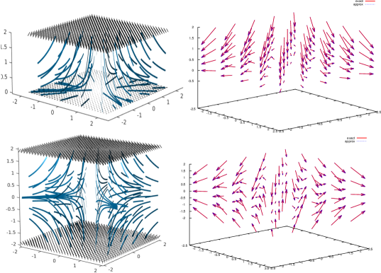
Figure 2. Example 5.1. (Left)Vector field 𝐮(x,y,z)=(x,y,2z)𝐮𝑥𝑦𝑧𝑥𝑦2𝑧\mathbf{u}(x,y,z)=(x,y,-2z) on (2,2)×(2,2)×(0,2)222202(-2,2)\times(-2,2)\times(0,2) and (2,2)×(2,2)×(2,2)222222(-2,2)\times(-2,2)\times(-2,2). (Right) Vector field approximation taking 𝐮0=(x,y,0)superscript𝐮0𝑥𝑦0\mathbf{u}^{0}=(x,y,0), the arrows -\!\!\!\!\blacktriangleright and >absent\cdots\!\!\!>, represents respectively exact and approximated vector field.

Let us consider an extension of the 2D field in Cervantes et al [5], namely 𝐮(x,y,z)=(x,y,2z)𝐮𝑥𝑦𝑧𝑥𝑦2𝑧\mathbf{u}(x,y,z)=(x,y,-2z) on the domains Ω1=(2,2)×(2,2)×(0,2)subscriptΩ1222202\Omega_{1}=(-2,2)\times(-2,2)\times(0,2) and Ω2=(2,2)×(2,2)×(2,2)subscriptΩ2222222\Omega_{2}=(-2,2)\times(-2,2)\times(-2,2) (which are shown on the left side of figure 2 in a stream ribbon style). Assume that 𝐮0(x,y,z)=(x,y,0)superscript𝐮0𝑥𝑦𝑧𝑥𝑦0\mathbf{u}^{0}(x,y,z)=(x,y,0), so that, in Ω1subscriptΩ1\Omega_{1} (domain with topography), we impose a No-Flow-Thrown boundary condition on ΓBsubscriptΓ𝐵\Gamma_{B}, while in Ω2subscriptΩ2\Omega_{2} a Dirichlet boundary condition is used on ΓBsubscriptΓ𝐵\Gamma_{B} (see figure 1).

The results are shown in table 1 and in the right hand side of figure 2. In the table 1, only the results for Ω1subscriptΩ1\Omega_{1} are displayed. The corresponding results for Ω2subscriptΩ2\Omega_{2} are nearly equivalent. The relative error and the approximated divergence, decreases as the number of centers increases. As expected, the condition number of Gram matrix increases. This is the well know and classic behavior of the schemes based on radial basis functions, the so called Schaback Uncertainty Principle [11].

N𝑁N c𝑐c κ(G)𝜅𝐺\kappa(G) u+subscript𝑢\nabla\cdot u_{+} u+𝐮2/𝐮2subscriptnormsubscript𝑢𝐮2subscriptnorm𝐮2\|u_{+}-\mathbf{u}\|_{2}/\|\mathbf{u}\|_{2}
27 0.001 2.252627e+18 4.679924e-05 2.707875e-05
125 0.001 5.801561e+19 1.088109e-06 5.342928e-06
512 0.001 1.195701e+20 7.873625e-08 6.961732e-08
Table 1. Example 5.1. Vector field approximation (𝐮+subscript𝐮\mathbf{u}_{+}) of 𝐮(x,y)=(x,y,2z)𝐮𝑥𝑦𝑥𝑦2𝑧\mathbf{u}(x,y)=(x,y,-2z) on (2,2)×(2,2)×(0,2)222202(-2,2)\times(-2,2)\times(0,2) using a set of equidistant centers.
Example 5.2.
Refer to caption
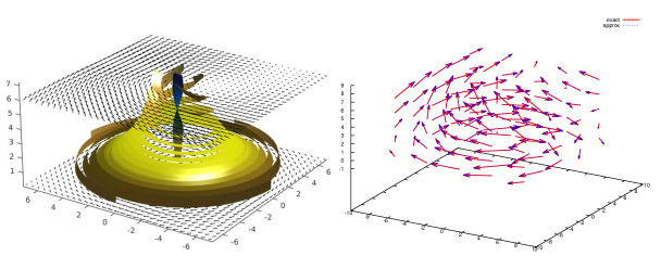
Figure 3. Example 5.2. (Left) Vector field 𝐮(x,y,z)=(2ye(x2+y2+z2)49,2xe(x2+y2+z2)49,1)𝐮𝑥𝑦𝑧2𝑦superscript𝑒superscript𝑥2superscript𝑦2superscript𝑧2492𝑥superscript𝑒superscript𝑥2superscript𝑦2superscript𝑧2491\mathbf{u}(x,y,z)=(2ye^{\frac{-(x^{2}+y^{2}+z^{2})}{49}},-2xe^{\frac{-(x^{2}+y^{2}+z^{2})}{49}},1) on (7,7)×(7,7)×(7,7)777777(-7,7)\times(-7,7)\times(-7,7). (Right) Vector field approximation taking taking 𝐮0(x,y,z)=(2ye(x2+y2+z2)49,2xe(x2+y2+z2)49,0)superscript𝐮0𝑥𝑦𝑧2𝑦superscript𝑒superscript𝑥2superscript𝑦2superscript𝑧2492𝑥superscript𝑒superscript𝑥2superscript𝑦2superscript𝑧2490\mathbf{u}^{0}(x,y,z)=(2ye^{-\frac{(x^{2}+y^{2}+z^{2})}{49}},-2xe^{-\frac{(x^{2}+y^{2}+z^{2})}{49}},0). The arrows -\!\!\!\!\blacktriangleright and >absent\cdots\!\!\!>, represents respectively exact and approximated vector field.

In this example, we approximate the (nontrivial) vortex type vector field in Benbourhim et al [1]. It is shown on the left side of figure 3 in a stream ribbon style, and is given by

𝐮(x,y,z)=(2ye(x2+y2+z2)49,2xe(x2+y2+z2)49,1)𝐮𝑥𝑦𝑧2𝑦superscript𝑒superscript𝑥2superscript𝑦2superscript𝑧2492𝑥superscript𝑒superscript𝑥2superscript𝑦2superscript𝑧2491\mathbf{u}(x,y,z)=(2ye^{-\frac{(x^{2}+y^{2}+z^{2})}{49}},-2xe^{-\frac{(x^{2}+y^{2}+z^{2})}{49}},1)

with Ω=(7,7)×(7,7)×(7,7)Ω777777\Omega=(-7,7)\times(-7,7)\times(-7,7). The initial field is taken as

𝐔0(x,y,z)=(2ye(x2+y2+z2)49,2xe(x2+y2+z2)49,0)superscript𝐔0𝑥𝑦𝑧2𝑦superscript𝑒superscript𝑥2superscript𝑦2superscript𝑧2492𝑥superscript𝑒superscript𝑥2superscript𝑦2superscript𝑧2490\mathbf{U}^{0}(x,y,z)=(2ye^{-\frac{(x^{2}+y^{2}+z^{2})}{49}},-2xe^{-\frac{(x^{2}+y^{2}+z^{2})}{49}},0)

In this case, we do not consider the topography and assume that vector field in the upper and lower regions are known. That is, Dirichlet boundary conditions for ΓTsubscriptΓ𝑇\Gamma_{T} and ΓBsubscriptΓ𝐵\Gamma_{B} are considered. The results are shown in table 2 and in the right hand side of figure 3.

N𝑁N c𝑐c κ(G)𝜅𝐺\kappa(G) u+subscript𝑢\nabla\cdot u_{+} u+𝐮2/𝐮2subscriptnormsubscript𝑢𝐮2subscriptnorm𝐮2\|u_{+}-\mathbf{u}\|_{2}/\|\mathbf{u}\|_{2}
27 0.01 6.468932e+09 -5.553522e-06 4.879887e-03
125 0.01 5.736571e+18 -6.975779e-03 2.968737e-05
512 0.01 1.057278e+20 -5.411860e-03 1.226800e-07
Table 2. Example 5.2. Vector field approximation (𝐮+subscript𝐮\mathbf{u}_{+}) of (2ye(x2+y2+z2)49,2xe(x2+y2+z2)49,1)2𝑦superscript𝑒superscript𝑥2superscript𝑦2superscript𝑧2492𝑥superscript𝑒superscript𝑥2superscript𝑦2superscript𝑧2491(2ye^{-\frac{(x^{2}+y^{2}+z^{2})}{49}},-2xe^{-\frac{(x^{2}+y^{2}+z^{2})}{49}},1) on (7,7)×(7,7)×(7,7)777777(-7,7)\times(-7,7)\times(-7,7) using a set of equidistant centers.
Example 5.3.
Refer to caption
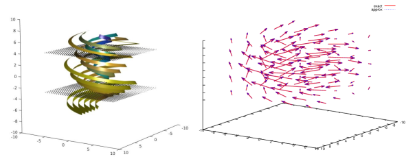
Figure 4. Example 5.3. (Left) Vector field 𝐮(x,y,z)=(2ye(x2+y2+z2)49εxz2,2xe(x2+y2+z2)49εxz2,εz22)𝐮𝑥𝑦𝑧2𝑦superscript𝑒superscript𝑥2superscript𝑦2superscript𝑧249𝜀𝑥𝑧22𝑥superscript𝑒superscript𝑥2superscript𝑦2superscript𝑧249𝜀𝑥𝑧2𝜀superscript𝑧22\mathbf{u}(x,y,z)=(2ye^{\frac{-(x^{2}+y^{2}+z^{2})}{49}}-\varepsilon\frac{xz}{2},-2xe^{\frac{-(x^{2}+y^{2}+z^{2})}{49}}-\varepsilon\frac{xz}{2},\varepsilon\frac{z^{2}}{2}) on (7,7)×(7,7)×(0,7)777707(-7,7)\times(-7,7)\times(0,7), for ε=0.1𝜀0.1\varepsilon=0.1. (Right) Vector field approximation, taking 𝐮0(x,y,z)=(2ye(x2+y2+z2)49εxz2,2xe(x2+y2+z2)49εyz2,0)superscript𝐮0𝑥𝑦𝑧2𝑦superscript𝑒superscript𝑥2superscript𝑦2superscript𝑧249𝜀𝑥𝑧22𝑥superscript𝑒superscript𝑥2superscript𝑦2superscript𝑧249𝜀𝑦𝑧20\mathbf{u}^{0}(x,y,z)=(2ye^{-\frac{(x^{2}+y^{2}+z^{2})}{49}}-\varepsilon\frac{xz}{2},-2xe^{-\frac{(x^{2}+y^{2}+z^{2})}{49}}-\varepsilon\frac{yz}{2},0). The arrows -\!\!\!\!\blacktriangleright and >absent\cdots\!\!\!>, represents respectively exact and approximated vector field.

In this last example we consider a variant of Example 5.2 to have a topography in the xy𝑥𝑦xy plane. Consequently the No-Flow-Through boundary condition is imposed on ΓBsubscriptΓ𝐵\Gamma_{B}.

The vector field is given by,

𝐮(x,y,z)=(2ye(x2+y2+z2)49εxz2,2xe(x2+y2+z2)49εyz2,εz22)𝐮𝑥𝑦𝑧2𝑦superscript𝑒superscript𝑥2superscript𝑦2superscript𝑧249𝜀𝑥𝑧22𝑥superscript𝑒superscript𝑥2superscript𝑦2superscript𝑧249𝜀𝑦𝑧2𝜀superscript𝑧22\mathbf{u}(x,y,z)=(2ye^{-\frac{(x^{2}+y^{2}+z^{2})}{49}}-\varepsilon\frac{xz}{2},-2xe^{-\frac{(x^{2}+y^{2}+z^{2})}{49}}-\varepsilon\frac{yz}{2},\varepsilon\frac{z^{2}}{2})

with Ω=(7,7)×(7,7)×(0,7)Ω777707\Omega=(-7,7)\times(-7,7)\times(0,7) and ε>0+𝜀0superscript\varepsilon>0\in\mathbb{R}^{+}. As before, the initial field is,

𝐮0(x,y,z)=(2ye(x2+y2+z2)49εxz2,2xe(x2+y2+z2)49εyz2,0).superscript𝐮0𝑥𝑦𝑧2𝑦superscript𝑒superscript𝑥2superscript𝑦2superscript𝑧249𝜀𝑥𝑧22𝑥superscript𝑒superscript𝑥2superscript𝑦2superscript𝑧249𝜀𝑦𝑧20\mathbf{u}^{0}(x,y,z)=(2ye^{-\frac{(x^{2}+y^{2}+z^{2})}{49}}-\varepsilon\frac{xz}{2},-2xe^{-\frac{(x^{2}+y^{2}+z^{2})}{49}}-\varepsilon\frac{yz}{2},0).

In the left hand side of figure 4, we show this vector filed for ε=0.1𝜀0.1\varepsilon=0.1 in a stream ribbon style. The corresponding results are shown in table 3 and in the right hand side of figure 4.

N𝑁N c𝑐c ϵitalic-ϵ\epsilon κ(G)𝜅𝐺\kappa(G) u+subscript𝑢\nabla\cdot u_{+} u+u2/u2subscriptnormsubscript𝑢𝑢2subscriptnorm𝑢2\|u_{+}-u\|_{2}/\|u\|_{2}
27 0.01 0.1 1.508177e+13 2.633422e-03 1.463895e-01
125 0.01 0.1 2.632883e+21 4.063153e-03 4.732374e-04
512 0.01 0.1 8.866826e+21 1.365358e-02 5.872183e-05
Table 3. Example 5.3. Vector field approximation (𝐮+subscript𝐮\mathbf{u}_{+}) of 𝐮(x,y)=(2ye(x2+y2+z2)49εxz2,2xe(x2+y2+z2)49εyz2,εz22)𝐮𝑥𝑦2𝑦superscript𝑒superscript𝑥2superscript𝑦2superscript𝑧249𝜀𝑥𝑧22𝑥superscript𝑒superscript𝑥2superscript𝑦2superscript𝑧249𝜀𝑦𝑧2𝜀superscript𝑧22\mathbf{u}(x,y)=(2ye^{-\frac{(x^{2}+y^{2}+z^{2})}{49}}-\varepsilon\frac{xz}{2},-2xe^{-\frac{(x^{2}+y^{2}+z^{2})}{49}}-\varepsilon\frac{yz}{2},\varepsilon\frac{z^{2}}{2}) on (7,7)×(7,7)×(0,7)777707(-7,7)\times(-7,7)\times(0,7) using a set of equidistant centers.

6. Conclusion

In this article we have introduced a mass consistent variational approach to approximate 3D vector fields from a set of prescribed scattered data values, whose vertical component is unknown. This problem is of great interest for meteorological applications and has been treated in the literature by several authors; see Ratto et al [6], for a recent review.

More precisely a first contribution of this article is that our approach, based on the adjoint method, let us build the adjusted field, as the unique solution along an appropriately chosen descent direction. A full analysis of the existence and uniqueness of the solution is proved within the proper Hilbertian setting. Boundary conditions for the adjoint equations arises naturally from the variational formulation in such a way that it is possible to build them according to the physical properties of the field. This point generalizes Sasaki’s pioneer approach, [4], which imposes in an heuristic way, particular boundary conditions. We prove in fact that Sasaki’s method is a particular case of our approach.

Several works, which uses classic techniques, like finite elements or finite differences, have appeared in the literature, to solve this problem, (see, [6]).

In order to avoid the computational expansive 3D mesh generation, some Radial Basis Functions (RBF) methods have been formulated; See Pepper, Rasmussen & Fyda [3], and Cervantes et al [5].

We recall the work of Benbourhim and Bouhamidi [1], that developed a smoothing algorithm for a given set of physically constrained prescribed data of vector fields in two and three dimensions. Although this is an important method, no boundary conditions can be imposed by this approach in an open bounded set in tow or three dimensions.

In our work a radial mesh free asymmetric collocation technique is used to discretize the adjoint equations in an open bounded domain. Inverse multiquadric kernels are used, thus providing exponential rate of convergence. Numerical experiments were designed to prove different boundary conditions, namely, when the field is tangential to the terrain and when no terrain is considered. In all cases, the numerical errors and the approximated value of the divergence are excellent for a small number of data.

Several points remains unsolved within the scope of this work. Among them, we mention its possible generalization to approximate vector fields having different physical properties, like zero rotational, or elasticity constrains. Also, in order to approximate real life data, this method could be restated as a smoothing approximant. Further work is in progress in these directions.

7. Acknowledgements

The authors would like to acknowledge to ECOS-NORD project number
000000000263116/M15M01 for financial support during this research. C. Gout thanks the M2NUM project which is co-financed by the European Union with the European regional development fund (ERDF, HN0002137) and by the Normandie Regional Council.”

References

  • [1] Benbourhim, Mohammed-Najib, and Abderrahman Bouhamidi. ”Pseudo-polyharmonic vectorial approximation for div-curl and elastic semi-norms.” Numerische Mathematik 109.3 (2008): 333-364.
  • [2] Duchon, Jean. ”Splines minimizing rotation-invariant semi-norms in Sobolev spaces.” Constructive theory of functions of several variables. Springer Berlin Heidelberg, 1977. 85-100.
  • [3] Pepper, Darrell W., Cody Rasmussen, and David Fyda. ”A meshless method using global radial basis functions for creating 3-D wind fields from sparse meteorological data.” Computer Assisted Methods in Engineering and Science 21.3-4 (2014): 233-243.
  • [4] Sasaki, Yoshikazu. ”An objective analysis based on the variational method.” Journal of the Meteorological Society of Japan. Ser. II 36.3 (1958): 77-88.
  • [5] Cabrera, Daniel A. Cervantes, et al. ”Vector field approximation using radial basis functions.” Journal of Computational and Applied Mathematics 240 (2013): 163-173.
  • [6] Ratto, C. F., et al. ”Mass-consistent models for wind fields over complex terrain: the state of the art.” Environmental Software 9.4 (1994): 247-268.
  • [7] Zeidler, Eberhard. Nonlinear Functional Analysis and Its Applications: III: Variational Methods and Optimization. Springer Science & Business Media, 2013.
  • [8] Sohr, Hermann. The Navier-Stokes equations: An elementary functional analytic approach. Springer Science & Business Media, 2012.
  • [9] Kansa, Edward J. ”Multiquadrics A scattered data approximation scheme with applications to computational fluid-dynamics II solutions to parabolic, hyperbolic and elliptic partial differential equations.” Computers & mathematics with applications 19.8-9 (1990): 147-161.
  • [10] Fornberg, Bengt, and Natasha Flyer. ”Accuracy of radial basis function interpolation and derivative approximations on 1-D infinite grids.” Advances in Computational Mathematics 23.1-2 (2005): 5-20.
  • [11] Schaback, Robert. ”Error estimates and condition numbers for radial basis function interpolation.” Advances in Computational Mathematics 3.3 (1995): 251-264.