A SICA compartmental model in epidemiology
with application to HIV/AIDS in Cape Verde

Abstract

We propose a new mathematical model for the transmission dynamics of the human immunodeficiency virus (HIV). Global stability of the unique endemic equilibrium is proved. Then, based on data provided by the “Progress Report on the AIDS response in Cape Verde 2015”, we calibrate our model to the cumulative cases of infection by HIV and AIDS from 1987 to 2014 and we show that our model predicts well such reality. Finally, a sensitivity analysis is done for the case study in Cape Verde. We conclude that the goal of the United Nations to end the AIDS epidemic by 2030 is a nontrivial task.

Keywords:

HIV/AIDS epidemiology, antiretroviral therapy (ART), SICA compartmental model, global stability, United Nations UNAIDS strategy.

MSC 2010:

34C60, 34D23, 92D30.

1 Introduction

The infection by human immunodeficiency virus (HIV) continues to be a major global public health issue, having claimed more than 34 million lives so far [26]. The most advanced stage of HIV infection is acquired immunodeficiency syndrome (AIDS). There is yet no cure or vaccine to AIDS. However, antiretroviral (ART) treatment improves health, prolongs life, and substantially reduces the risk of HIV transmission. In both high-income and low-income countries, the life expectancy of patients infected with HIV who have access to ART is now measured in decades, and might approach that of uninfected populations in patients who receive an optimum treatment (see [8] and references cited therein). However, ART treatment still presents substantial limitations: does not fully restore health; treatment is associated with side effects; the medications are expensive; and is not curative. According to the Joint United Nations Programme on HIV and AIDS (UNAIDS), the main advocate for accelerated, comprehensive and coordinated global action on the HIV/AIDS epidemic, the number of people living with HIV continues to increase, in large part because more people are accessing ART therapy globally. In 2015, 15.8 million people were accessing treatment. New HIV infections have fallen by 35% since 2000 and AIDS-related deaths have fallen by 42% since the peak in 2004. In 2000, fewer than 1% of people living with HIV in low- and middle-income countries had access to treatment. In 2014, the global coverage of people receiving ART therapy was 40%. However, in 2014, around 2 million people were newly infected with HIV and 1.2 million people died of AIDS-related illnesses. Of the 36.9 million people living with HIV globally in 2014, 17.1 million did not know they had the virus and were not aware of the need to be reached with HIV testing services. Around 22 million do not had access to HIV treatment, including 1.8 million children [24].

Cape Verde is an island country spanning an archipelago of 10 volcanic islands in the central Atlantic Ocean. Located 570 kilometres (350 miles) off the coast of Western Africa, the islands cover a combined area of slightly over 4,000 square kilometres (1,500 square miles). Since the early 1990s, Cape Verde has been a stable representative democracy, and remains one of the most developed and democratic countries in Africa. Its population is of around 506,000 residents with a sizeable diaspora community across all the world, outnumbering the inhabitants on the islands. Such facts make Cape Verde an important case study, with global implications [21].

In 2014, 409 new HIV cases were reported in Cape Verde, accumulating a total of 4,946 cases. Of this total, 1,766 developed AIDS and 1,066 have died. The municipality with more cases was Praia, followed by Santa Catarina (Santiago island) and São Vicente. Cape Verde has developed a Strategic National Plan to fight against AIDS, which includes ART treatment, monitoring of patients, prevention actions and HIV testing. From the first diagnosis of AIDS in 1986, Cape Verde got significant progress in the fight, prevention and treatment of HIV/AIDS [20].

Mathematical models, based on the underlying transmission mechanism of the HIV, can help the medical and scientific community to understand and anticipate its spread in different populations and evaluate the potential effectiveness of different approaches for bringing the epidemic under control [12]. Several mathematical models have been proposed for HIV/AIDS transmission dynamics: see, e.g., [1, 2, 3, 5, 6, 9, 10, 12, 13, 17, 18] and references cited therein.

In this paper, based on [23], we propose and analyse a mathematical model for the transmission dynamics of HIV and AIDS. Our aim is to show that a simpler mathematical model than the one of [23] can help to clarify some of the essential relations between epidemiological factors and the overall pattern of the AIDS epidemic, as it was stated in [17]. Our model considers ART treatment of HIV-infected individuals with and without AIDS symptoms. The HIV-infected individuals with no AIDS symptoms that start ART treatment move into the class of individuals that respect carefully ART treatment and stay in what we call a chronic stage of the infection. We assume that individuals in the chronic class have the same expectancy of life as non HIV infected individuals. Our model is then calibrated to the cumulative cases of infection by HIV and AIDS in Cape Verde, from 1987 to 2014, as reported in [20]. We show that our model predicts well such reality. A sensitivity analysis is then carried out, for some of the model parameters, and some conclusions for Cape Verde and worldwide inferred.

The paper is organized as follows. The model is formulated and analysed in Section 2. In Section 3, we prove the global stability of the unique endemic equilibrium whenever the basic reproduction number is greater than one. In Section 4, we do a sensitivity analysis of the basic reproduction number. Finally, in Section 5 we apply our model to HIV/AIDS Cape Verde infection data from the period of 1987 to 2014 and some conclusions are derived in Section 6.

2 The SICA model for HIV/AIDS transmission

In this section we propose and analyse a mathematical model for HIV/AIDS transmission with varying population size in a homogeneously mixing population. The model is based on that of [23] and subdivides the human population into four mutually-exclusive compartments: susceptible individuals ($S$); HIV-infected individuals with no clinical symptoms of AIDS (the virus is living or developing in the individuals but without producing symptoms or only mild ones) but able to transmit HIV to other individuals ($I$); HIV-infected individuals under ART treatment (the so called chronic stage) with a viral load remaining low ($C$); and HIV-infected individuals with AIDS clinical symptoms ($A$). The total population at time $t$, denoted by $N(t)$, is given by

$$N(t)=S(t)+I(t)+C(t)+A(t).$$

The susceptible population is increased by the recruitment of individuals into the population, assumed susceptible, at a rate $\Lambda$. All individuals suffer from natural death, at a constant rate $\mu$. Although individuals in the chronic stage, with a low viral load and under ART treatment, can still transmit HIV infection, as ART greatly reduces the risk of transmission and individuals that take ART treatment correctly are aware of their health status, we assume that individuals in the class $C$ do not have risky behaviours for HIV transmission and do not transmit HIV virus. We also assume that individuals with AIDS clinical symptoms $A$ are responsible and do not have any behaviour that can transmit HIV infection or, in other cases, are too sick to have a risky behaviour. Based on these two assumptions, susceptible individuals acquire HIV infection by following effective contact with individuals in the class $I$ at a rate $\lambda=\beta\frac{I}{N}$, where $\beta$ is the effective contact rate for HIV transmission. We assume that HIV-infected individuals with and without AIDS symptoms have access to ART treatment. HIV-infected individuals with no AIDS symptoms $I$ progress to the class of individuals with HIV infection under ART treatment $C$ at a rate $\phi$, and HIV-infected individuals with AIDS symptoms are treated for HIV at rate $\alpha$. We assume that an HIV-infected individual with AIDS symptoms $A$ that starts treatment moves to the class of HIV-infected individuals $I$ and he will move to the chronic class $C$ only if the treatment is maintained. HIV-infected individuals with no AIDS symptoms $I$ that do not take ART treatment progress to the AIDS class $A$ at rate $\rho$. We assume that only HIV-infected individuals with AIDS symptoms $A$ suffer from an AIDS induced death, at a rate $d$. These assumptions are translated in the following mathematical model:

$$\begin{cases}\dot{S}(t)=\Lambda-\beta\frac{I(t)}{N(t)}S(t)-\mu S(t),\\[5.69046pt] \dot{I}(t)=\beta\frac{I(t)}{N(t)}S(t)-(\rho+\phi+\mu)I(t)+\alpha A(t)+\omega C(t),\\[5.69046pt] \dot{C}(t)=\phi I(t)-(\omega+\mu)C(t),\\[5.69046pt] \dot{A}(t)=\rho\,I(t)-(\alpha+\mu+d)A(t).\end{cases}$$ (1)

The epidemiological scheme of (1) is given in Figure 1.

Figure 1: Epidemiological scheme of the SICA mathematical model (1).

Consider the biologically feasible region

$$\Omega=\left\{(S,I,C,A)\in{\mathbb{R}}^{4}_{+0}\,|\,0\leq S+I+C+A\leq\frac{\Lambda}{\mu}\right\}.$$

Using a standard comparison theorem (see [15]) one can easily show that $N(t)\leq\frac{\Lambda}{\mu}$ if $N(0)\leq\frac{\Lambda}{\mu}$. Thus, the region $\Omega$ is positively invariant. Hence, it is sufficient to consider the dynamics of the flow generated by (1) in $\Omega$. In this region, the model is epidemiologically and mathematically well posed in the sense of [11]. In other words, every solution of the model (1) with initial conditions in $\Omega$ remains in $\Omega$ for all $t>0$. For the persistence of the host population and disease we refer the reader to [23, Section 3.1.1]. Precisely, the disease is persistent in the population if the fraction of the infected and AIDS cases is bounded away from zero. If the population dies out and the fraction of the infected and AIDS remains bounded away from zero, the disease still remains persistent in the population. The model (1) has a disease-free equilibrium given by

$$\Sigma_{0}=\left(S^{0},I^{0},C^{0},A^{0}\right)=\left(\frac{\Lambda}{\mu},0,0,0\right).$$

The basic reproduction number $R_{0}$, which represents the expected average number of new HIV infections produced by a single HIV-infected individual when in contact with a completely susceptible population, is easily computed by the van den Driessche and Watmough approach [25]:

$$R_{0}=\frac{\beta\xi_{1}\xi_{2}}{\mu\left[\xi_{2}(\rho+\xi_{1})+\xi_{1}\phi+\rho d\right]+\rho\omega d}=\frac{\mathcal{D}}{\mathcal{N}},$$ (2)

where

$$\xi_{1}=\alpha+\mu+d\ \text{ and }\ \xi_{2}=\omega+\mu.$$

Lemma 2.1 (See [23]).

The disease free equilibrium $\Sigma_{0}$ is globally asymptotically stable if $R_{0}<1$. If $R_{0}>1$, then the disease free equilibrium $\Sigma_{0}$ is unstable.

To find conditions for the existence of an equilibrium $\Sigma^{*}=\left(S^{*},I^{*},C^{*},A^{*}\right)$ for which HIV is endemic in the population (i.e., at least one of $I^{*}$, $C^{*}$ or $A^{*}$ is nonzero), the equations in (1) are solved in terms of the force of infection at steady-state ($\lambda^{*}$), given by

$$\lambda^{*}=\frac{\beta I^{*}}{N^{*}}.$$ (3)

Setting the right-hand sides of the model (1) to zero (and noting that $\lambda=\lambda^{*}$ at equilibrium) gives

$$S^{*}=\frac{\Lambda}{\lambda^{*}+\mu},\quad I^{*}=\frac{\lambda^{*}\Lambda\xi_{1}\xi_{2}}{D},\quad C^{*}=\frac{\phi\lambda^{*}\Lambda\xi_{1}}{D},\quad A^{*}=\frac{\rho\lambda^{*}\Lambda\xi_{2}}{D}$$ (4)

with $D=(\lambda^{*}+\mu)\left[\mu\left(\xi_{2}(\rho_{1}+\xi_{1})+\xi_{1}\phi+\rho d\right)+\rho\omega d\right]$. Using (4) in the expression for $\lambda^{*}$ in (3) shows that the nonzero (endemic) equilibria of the model satisfies

$$\lambda^{*}=\mu(R_{0}-1).$$

The force of infection at the steady-state $\lambda^{*}$ is positive only if $R_{0}>1$. Therefore, system (1) has a unique endemic equilibrium whenever $R_{0}>1$. This is in agreement with [23, Lemma 3.7].

3 Global stability of the endemic equilibrium

In this section, we prove the global stability of the endemic equilibrium $\Sigma^{*}$. We assume that each variable $S$, $I$, $C$ and $A$ represents the corresponding proportion of the total population and consider the following system:

$$\begin{cases}\dot{S}(t)=\Lambda-\beta I(t)S(t)-\mu S(t),\\[5.69046pt] \dot{I}(t)=\beta I(t)S(t)-(\rho+\phi+\mu)I(t)+\alpha A(t)+\omega C(t),\\[5.69046pt] \dot{C}(t)=\phi I(t)-(\omega+\mu)C(t),\\[5.69046pt] \dot{A}(t)=\rho\,I(t)-(\alpha+\mu+d)A(t).\end{cases}$$ (5)

Let us start by defining the region

$$\Omega_{0}=\left\{(S,I,C,A)\in\Omega\,|\,I=C=A=0\right\}.$$

Consider the following Lyapunov function:

$$V=S-S^{*}-S^{*}\ln\left(\frac{S}{S^{*}}\right)+I-I^{*}-I^{*}\ln\left(\frac{I}{I^{*}}\right)+\frac{\omega}{\xi_{2}}\left(C-C^{*}-C^{*}\ln\left(\frac{C}{C^{*}}\right)\right)\\ +\frac{\alpha}{\xi_{1}}\left(A-A^{*}-A^{*}\ln\left(\frac{A}{A^{*}}\right)\right).$$

Differentiating $V$ with respect to time gives

$$\dot{V}=\left(1-\frac{S^{*}}{S}\right)\dot{S}+\left(1-\frac{I^{*}}{I}\right)\dot{I}+\frac{\omega}{\xi_{2}}\left(1-\frac{C^{*}}{C}\right)\dot{C}+\frac{\alpha}{\xi_{1}}\left(1-\frac{A^{*}}{A}\right)\dot{A}.$$

Let $\xi_{3}=\rho+\phi+\mu$. Substituting the expressions for the derivatives in $\dot{V}$, it follows from (5) that

$$\dot{V}=\left(1-\frac{S^{*}}{S}\right)\left[\Lambda-\beta IS-\mu S\right]+\left(1-\frac{I^{*}}{I}\right)\left[\beta IS-\xi_{3}I+\alpha A+\omega C\right]\\ +\frac{\omega}{\xi_{2}}\left(1-\frac{C^{*}}{C}\right)\left[\phi I-\xi_{2}C\right]+\frac{\alpha}{\xi_{1}}\left(1-\frac{A^{*}}{A}\right)\left[\rho I-\xi_{1}A\right].$$ (6)

Using the relation $\Lambda=\beta I^{*}S^{*}+\mu S^{*}$, we have from the first equation of system (5) at steady-state that (6) can be written as

$$\dot{V}=\left(1-\frac{S^{*}}{S}\right)\left[\beta I^{*}S^{*}+\mu S^{*}-\beta IS-\mu S\right]+\left(1-\frac{I^{*}}{I}\right)\left[\beta IS-\xi_{3}I+\alpha A+\omega C\right]\\ +\frac{\omega}{\xi_{2}}\left(1-\frac{C^{*}}{C}\right)\left[\phi I-\xi_{2}C\right]+\frac{\alpha}{\xi_{1}}\left(1-\frac{A^{*}}{A}\right)\left[\rho I-\xi_{1}A\right],$$

which can then be simplified to

$$\dot{V}=\beta I^{*}S^{*}\left(1-\frac{S^{*}}{S}\right)+\mu S^{*}\left(2-\frac{S}{S^{*}}-\frac{S^{*}}{S}\right)+S^{*}\beta I-\xi_{3}I+\frac{\omega}{\xi_{2}}\phi I+\frac{\alpha}{\xi_{1}}\rho I\\ -\frac{I^{*}}{I}\left[\beta IS-\xi_{3}I+\alpha A+\omega C\right]-\frac{\omega}{\xi_{2}}\frac{C^{*}}{C}\left(\phi I-\xi_{2}C\right)-\frac{\alpha}{\xi_{1}}\frac{A^{*}}{A}\left(\rho I-\xi_{1}A\right).$$

Using the relations at the steady state

$$I^{*}=\frac{\beta I^{*}S^{*}+\alpha A^{*}+\omega C^{*}}{\xi_{3}},\quad C^{*}=\frac{\phi I^{*}}{\xi_{2}},\quad A^{*}=\frac{\rho I^{*}}{\xi_{1}},$$

we have

$$\dot{V}=\beta I^{*}S^{*}\left(1-\frac{S^{*}}{S}\right)+\mu S^{*}\left(2-\frac{S}{S^{*}}-\frac{S^{*}}{S}\right)-\frac{I^{*}}{I}\left(\beta IS-\xi_{3}I+\alpha A+\omega C\right)\\ -\frac{\omega}{\xi_{2}}\frac{C^{*}}{C}\left(\phi I-\xi_{2}C\right)-\frac{\alpha}{\xi_{1}}\frac{A^{*}}{A}\left(\rho I-\xi_{1}A\right).$$

Simplifying further the previous equations, we finally have

$$\begin{split}\dot{V}&=\left(\beta I^{*}S^{*}+\mu S^{*}\right)\left(2-\frac{S^{*}}{S}-\frac{S}{S^{*}}\right)\\ &\quad+\omega C^{*}\left(1-\frac{C}{C^{*}}\frac{I^{*}}{I}\right)+\alpha A^{*}\left(1-\frac{A}{A^{*}}\frac{I^{*}}{I}\right)\\ &\quad+\frac{\omega\phi}{\xi_{2}}I^{*}\left(1-\frac{C^{*}}{C}\frac{I}{I^{*}}\right)+\frac{\alpha\rho}{\xi_{1}}I^{*}\left(1-\frac{A^{*}}{A}\frac{I}{I^{*}}\right),\end{split}$$

which is less than or equal to zero by the arithmetic mean-geometric mean inequality. Therefore, we have $\dot{V}\leq 0$ with equality holding only if $S=S^{*}$ and $\frac{I}{I^{*}}=\frac{C}{C^{*}}=\frac{A}{A^{*}}$. By LaSalle’s invariance principle [16], the omega limit set of each solution lies in an invariant set contained in

$$\mathcal{P}=\left\{(S,I,C,A)\,|\,S=S^{*},\frac{I}{I^{*}}=\frac{C}{C^{*}}=\frac{A}{A^{*}}\right\}.$$

Since $S$ must remain constant at $S^{*}$, $\dot{S}$ is zero. This implies that $I=I^{*}$, making $\frac{I}{I^{*}}$ equal to one. Thus, $C=C^{*}$ and $A=A^{*}$. Hence, the only invariant set contained in $\mathcal{P}$ is the singleton $\{\Sigma^{*}\}$. This shows that the endemic equilibrium $\Sigma^{*}$ is the only solution that intersects $\Omega$. We have just proved that if $R_{0}>1$, then the unique endemic equilibrium $\Sigma^{*}$ is globally asymptotically stable on $\Omega\backslash\Omega_{0}$. This result is summarized in the following theorem.

Theorem 3.1.

The unique endemic equilibrium $\Sigma^{*}$ of model (5) is globally asymptotically stable in $\Omega\backslash\Omega_{0}$ whenever $R_{0}>1$.

4 Sensitivity of the basic reproduction number

The sensitivity of the basic reproduction number $R_{0}$ is an important issue because it determines the model robustness to parameter values. Let us examine the sensitivity of $R_{0}$ with respect to some parameters. We start by examining the sensitivity of $R_{0}$ with respect to $\beta$.

Proposition 4.1.

The basic reproduction number $R_{0}$ increases with $\beta$.

Proof.

The results follows immediately from the fact that

$$\frac{\partial R_{0}}{\partial\beta}>0$$

for any value of the parameters. ∎

The partial derivatives of $R_{0}$ with respect to the treatment rate for HIV-infected individuals with no symptoms of AIDS and HIV-infected individuals with AIDS symptoms, $\phi$ and $\alpha$, respectively, are given by

$$\frac{\partial R_{0}}{\partial\phi}=-\frac{\beta\mu\xi_{1}^{2}\xi_{2}}{\mathcal{D}^{2}},\qquad\frac{\partial R_{0}}{\partial\alpha}=\frac{\beta\rho\xi_{2}^{2}(\mu+d)}{\mathcal{D}^{2}}.$$ (7)

It follows from (7) that $\frac{\partial R_{0}}{\partial\phi}<0$ and $\frac{\partial R_{0}}{\partial\alpha}>0$ for any value of the parameters. Therefore, the treatment of HIV-infected individuals with no symptoms of AIDS, $I$, has always a positive impact in reducing the HIV burden. On the other hand, the treatment of HIV-infected individuals increases the number of HIV-infected individuals, explained because when they start ART treatment their expectancy of life increases and there will be more people living with HIV-infection with no AIDS symptoms. This is summarized in the following result.

Proposition 4.2.

The basic reproduction number $R_{0}$ decreases with $\phi$ and increases with $\alpha$.

The partial derivatives of $R_{0}$ with respect to the default treatment rates $\rho$ and $\omega$ are given, respectively, by

$$\frac{\partial R_{0}}{\partial\rho}=-\frac{\beta\xi_{1}\xi_{2}^{2}(\mu+d)}{\mathcal{D}^{2}},\qquad\frac{\partial R_{0}}{\partial\omega}=\frac{\beta\phi\mu\xi_{1}^{2}}{\mathcal{D}^{2}}.$$

Thus, the basic reproduction number increases with the default treatment rate of individuals in the chronic class $\omega$ and decreases with the default treatment rate of individuals in the class $I$. This makes sense because the lack of ART treatment implies a progression to AIDS disease. This is stated in the following result.

Proposition 4.3.

The basic reproduction number $R_{0}$ decreases with $\rho$ and increases with $\omega$.

The sensitivity of a variable (in our case of interest, $R_{0}$) with respect to model parameters is sometimes measured by the so called sensitivity index.

Definition 4.1 (cf. [7, 14]).

The normalized forward sensitivity index of a variable $\upsilon$ that depends differentiably on a parameter $p$ is defined by

$$\Upsilon_{p}^{\upsilon}:=\frac{\partial\upsilon}{\partial p}\times\frac{p}{|\upsilon|}.$$ (8)

Remark 4.1.

To the most sensitive parameter $p$ it corresponds a normalized forward sensitivity index of one or minus one, that is, $\Upsilon_{p}^{\upsilon}=\pm 1$. If $\Upsilon_{p}^{\upsilon}=+1$, then an increase (decrease) of $p$ by $x\%$ increases (decreases) $\upsilon$ by $x\%$; if $\Upsilon_{p}^{\upsilon}=-1$, then an increase (decrease) of $p$ by $x\%$ decreases (increases) $\upsilon$ by $x\%$.

From (2) and Definition 4.1, it is easy to derive the normalized forward sensitivity index of $R_{0}$ with respect to $\beta$.

Proposition 4.4.

The normalized forward sensitivity index of $R_{0}$ with respect to $\beta$ is $1$: $\Upsilon_{\beta}^{R_{0}}=1$.

Proof.

It is a direct consequence of (2) and (8). ∎

The sensitivity index of $R_{0}$ with respect to $\phi$, $\rho$, $\alpha$ and $\omega$ is given, respectively, by

$$\Upsilon_{\phi}^{R_{0}}=-\phi\frac{\mu C_{3}}{\mathcal{D}},\quad\Upsilon_{\rho}^{R_{0}}=-\rho\frac{C_{2}(\mu+d)}{\mathcal{D}},\quad\Upsilon_{\alpha}^{R_{0}}=\alpha\frac{\rho C_{2}(\mu+d)}{C_{3}\mathcal{D}},\quad\Upsilon_{\omega}^{R_{0}}=\omega\frac{\phi\mu C_{3}}{C_{2}\mathcal{D}}.$$

In Section 5 we compute the previous sensitivity indexes for the Cape Verde HIV/AIDS data.

5 Model application to Cape Verde HIV/AIDS data

In this section, we calibrate our model (1) to the cumulative cases of infection by HIV and AIDS from 1987 to 2014 and we show that it predicts well this reality. In Table 1, the cumulative cases of infection by HIV and AIDS in Cape Verde are depicted for the years 1987–2014 [20].

Year	1987	1988	1989	1990	1991	1992	1993	1994	1995	1996
HIV/AIDS	61	107	160	211	244	303	337	358	395	432
Year	1997	1998	1999	2000	2001	2002	2003	2004	2005	2006
HIV/AIDS	471	560	660	779	913	1064	1233	1493	1716	2015
Year	2007	2008	2009	2010	2011	2012	2013	2014
HIV/AIDS	2334	2610	2929	3340	3739	4090	4537	4946

Table 1: Cumulative cases of infection by HIV/AIDS in Cape Verde in the period 1987–2014 [20].

Taking into account the data from Table 1, we estimate empirically the value of the HIV transmission rate to be $\beta=0.857$. Searching for the optimal value of $\beta$ in the interval $[0.8,0.9]$ with respect to the $l_{2}$ norm, we find that the optimal value of $\beta$ is $\beta=0.866$, with an error equal to 0.507% individuals per year with respect to the initial total population. In all our simulations we choose $\beta=0.866$. Moreover, we consider the initial conditions (9) based on [20, 27]:

$$S_{0}=S(0)=338923\,,\quad I_{0}=I(0)=61\,,\quad C_{0}=C(0)=0\,,\quad A_{0}=A(0)=0.$$ (9)

The values of the parameters $\rho=0.1$ and $\alpha=0.33$ are taken from [22] and [4], respectively. We assume that after one year, the HIV infected individuals $I$ that are under ART treatment have a low viral load [19] and, therefore, are transferred to the class $C$. In agreement, we take $\phi=1$. It is well known that taking ART therapy is a long-term commitment. In our simulations we assume that the default treatment rate for $C$ individuals is approximately 11 years ($1/\omega$ years to be precise). Following the World Bank data [27], the recruitment and the natural death rates are assumed to take the values $\Lambda=10724$ and $\mu=1/69.54$. Finally, the AIDS induced death rate is assume to be $d=1$ based on [28]. All the considered parameter values are resumed in Table 2.

Symbol	Description	Value	References
$N(0)$	Initial population	$338984$	[27]
$\Lambda$	Recruitment rate	$10724$	[27]
$\mu$	Natural death rate	$1/69.54$	[27]
$\beta$	HIV transmission rate	$0.866$	Estimated
$\phi$	HIV treatment rate for $I$ individuals	$1$	[19]
$\rho$	Default treatment rate for $I$ individuals	$0.1$	[22]
$\alpha$	AIDS treatment rate	$0.33$	[4]
$\omega$	Default treatment rate for $C$ individuals	$0.09$	Assumed
$d$	AIDS induced death rate	$1$	[28]

Table 2: Parameters of the HIV/AIDS model (1) for Cape Verde.

In Figure 2, we observe that model (1) fits the real data reported in Table 1. The cumulative cases described by model (1) are given by $I(t)+C(t)+A(t)+\mu\left(I(t)+C(t)\right)+(\mu+d)\left(A(t)\right)$ for $t\in[0,27]$, which corresponds to the interval of time between the years of 1987 ($t=0$) and 2014 ($t=27$).

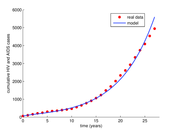
Figure 2: Model (1) fitting the data of cumulative cases of HIV and AIDS infection in Cape Verde between 1987 and 2014 [20].

The parameter values from Table 2 correspond to a basic reproduction number $R_{0}=3.8049$. Figure 3 illustrates, numerically, the global stability of the endemic equilibrium. For this reason, we consider different initial conditions, in different regions of the plane, sufficiently far a way from the endemic equilibrium $(S^{*},I^{*},C^{*},A^{*})=(146000,37894,363040,2818.7)$.

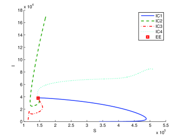
(a) $(S,I)$

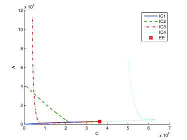
(b) $(C,A)$

Figure 3: (a) Susceptible individuals versus HIV-infected individuals with no clinical symptoms of AIDS. (b) HIV-infected individuals under treatment for HIV infection versus HIV-infected individuals with AIDS clinical symptoms. Both figures consider initial conditions $IC1=(S_{0},I_{0},C_{0},A_{0})$, $IC2=(S_{0}/2,I_{0}+S_{0}/2,C_{0}+10^{4},A_{0}+4\times 10^{4})$, $IC3=(S_{0}/3,I_{0},C_{0}+4\times 10^{4},A_{0}+S_{0}/3)$, and $IC4=(3S_{0}/2,I_{0}+S_{0}/4,C_{0}+5\times 10^{5},A_{0}+S_{0}/5)$. EE denotes the endemic equilibrium $(S^{*},I^{*},C^{*},A^{*})=(146000,37894,363040,2818.7)$.

In Table 3, we present the sensitivity index of parameters $\beta$, $\phi$, $\rho$, $\alpha$ and $\omega$ computed for the parameter values given in Table 2.

Parameter	Sensitivity index
$\beta$	+1
$\phi$	$-0.6053$
$\rho$	$-0.3315$
$\alpha$	$+0.0814$
$\omega$	$+0.5219$

Table 3: Sensitivity index of $R_{0}$ for parameter values given in Table 2.

6 Conclusion

In this paper, we proposed a nonlinear mathematical model for HIV/AIDS transmission with varying population size in a homogeneously mixing population. The model was analysed for the particular situation where only HIV-infected individuals with no AIDS symptoms, which are not under ART treatment, transmit HIV virus. However, the global stability result can be easily extended to the case where individuals under ART treatment and individuals with AIDS disease also transmit HIV virus. We have shown that the proposed model describes very well the reality given by the data of HIV/AIDS infection in Cape Verde from 1987 to 2014. We conclude that, with the parameter values of Table 2, the endemic equilibrium for Cape Verde is $(S^{*},I^{*},C^{*},A^{*})=(146000,37894,363040,2818.7)$, which is not an encouraging prediction. Indeed, the number of individuals with HIV-infection and AIDS disease is relatively big and increasing and does not converge to the UNAIDS worldwide goal of ending the AIDS epidemic by 2030 [24]. From the sensitivity index of the basic reproduction number with respect to treatment rates for HIV-infected individuals with no AIDS symptoms, we may conclude that it is important to invest in providing conditions to HIV-infected individuals to maintain, correctly, the ART treatment. Analogously, HIV-infected individuals with AIDS disease should be supported in order to start ART treatment as soon as possible. All the measures that help to reduce the default treatment should be supported. Finally, it is essential to reduce HIV transmission. We observed that the transmission rate is the parameter that most affects the basic reproduction number.

References

- [1] R. M. Anderson, The role of mathematical models in the study of HIV transmission and the epidemiology of AIDS, J. AIDS 1 (1988), 241–256.
- [2] R. M. Anderson, S. P. Blythe, S. Gupta, E. Konings, The Transmission Dynamics of the Human Immunodeficiency Virus Type 1 in the Male Homosexual Community in the United Kingdom: The Influence of Changes in Sexual Behavior, Philos. Trans. R. Soc. Lond. B 325 (1989), 45–98.
- [3] C. P. Bhunu, W. Garira, G. Magombedze, Mathematical analysis of a two strain HIV/AIDS model with antiretroviral treatment, Acta Biotheor. 57 (2009), 361–381.
- [4] C. P. Bhunu, W. Garira and Z. Mukandavire, Modeling HIV/AIDS and tuberculosis coinfection, Bul. Math. Biol. 71 (2009), 1745–1780.
- [5] C. P. Bhunu, S. Mushayabasa, H. Kojouharov, J. M. Tchuenche, Mathematical Analysis of an HIV/AIDS Model: Impact of Educational Programs and Abstinence in Sub-Saharan Africa, J. Math. Model. Algor. 10 (2011), 31–55.
- [6] L. Cai, X. Li, M. Ghosh, B. Guo, Stability analysis of an HIV/AIDS epidemic model with treatment, J. Comput. Appl. Math. 229 (2009), 313–323.
- [7] N. Chitnis, J. M. Hyman, J. M. Cushing, Determining important parameters in the spread of malaria through the sensitivity analysis of a mathematical model, Bull. Math. Biol. 70 (2008), no. 5, 1272–1296.
- [8] S. G. Deeks, S. R. Lewin and D. V. Havlir, The end of AIDS: HIV infection as a chronic disease, The Lancet 382 (2013), 1525–1533.
- [9] R. M. Granich, C. F. Gilks, C. Dye, K. M. De Cock, B. G. Williams, Universal voluntary HIV testing with immediate antiretroviral therapy as a strategy for elimination of HIV transmission: a mathematical model, The Lancet 373 (2009), 48–57.
- [10] D. Greenhalgh, M. Doyle, F. Lewis, A mathematical model of AIDS and condom use, IMA J. Math. Appl. Med. Biol. 18 (2001), 225–262.
- [11] H. W. Hethcote, The mathematics of infectious diseases, SIAM Rev. 42 (2000), 599–653.
- [12] J. M. Hyman, E. A. Stanley, Using mathematical models to understand the AIDS epidemic, Math. Biosci. 90 (1988), 415–473.
- [13] H. Joshi, S. Lenhart, K. Albright, K. Gipson, Modeling the effect of information campaigns on the HIV epidemic in Uganda, Math. Biosci. Eng. 5 (2008), 757–770.
- [14] Q. Kong, Z. Qiu, Z. Sang, Y. Zou, Optimal control of a vector-host epidemics model, Math. Control Relat. Fields 1 (2011), no. 4, 493–508.
- [15] V. Lakshmikantham, S. Leela, A. A. Martynyuk, Stability Analysis of Nonlinear Systems, Marcel Dekker, Inc., New York and Basel, 1989.
- [16] J. P. LaSalle, The Stability of Dynamical Systems. In: Regional Conference Series in Applied Mathematics, SIAM, Philadelphia, 1976.
- [17] R. M. May, R. M. Anderson, Transmission dynamics of HIV infection, Nature 326 (1987), 137–142.
- [18] J. Musgrave, J. Watmough, Examination of a simple model of condom usage and individual withdrawal for the HIV epidemic, Math. Biosci. Eng. 6 (2009), 363–376.
- [19] A. S. Perelson et al., Decay characteristics of HIV-1-infected compartments during combination therapy, Nature 387 (1997), 188–191.
- [20] República de Cabo Verde, Rapport de Progrès sur la riposte au SIDA au Cabo Verde – 2015, Comité de Coordenação do Combate a Sida, 2015.
- [21] H. S. Rodrigues, M. T. T. Monteiro, D. F. M. Torres, Dengue in Cape Verde: vector control and vaccination, Math. Popul. Stud. 20 (2013), no. 4, 208–223. arXiv:1204.0544
- [22] O. Sharomi, C. Podder, A. B. Gumel, Mathematical analysis of the transmission dynamics of HIV/TB co-infection in the presence of treatment, Math. Biosci. Eng. 5 (2008), 145–174.
- [23] C. J. Silva, D. F. M. Torres, A TB-HIV/AIDS coinfection model and optimal control treatment, Discrete Contin. Dyn. Syst. 35 (2015), no. 9, 4639–4663. arXiv:1501.03322
- [24] UNAIDS, AIDS by the numbers 2015, UNAIDS, Geneva, 2015.
- [25] P. van den Driessche, J. Watmough, Reproduction numbers and subthreshold endemic equilibria for compartmental models of disease transmission, Math. Biosc. 180 (2002), 29–48.
- [26] WHO, HIV/AIDS Fact Sheet no. 360, 2015.
- [27] World Bank Data, Cabo Verde, World Development Indicators, http://data.worldbank.org/country/cape-verde
- [28] M. Zwahlen, M. Egger, Progression and mortality of untreated HIV-positive individuals living in resource-limited settings: update of literature review and evidence synthesis, Report on UNAIDS obligation no HQ/05/422204, 2006.