Gustafson integrals for $SL(2,\mathbb{C})$ spin magnet.

Abstract

It was observed recently that the multidimensional Mellin–Barnes integrals (Gustafson’s integrals) arise naturally in studies of the $SL(2,R)$ spin chain models. We extend this analysis to the noncompact $SL(2,\mathbb{C})$ spin magnets and obtain integrals which generalize Gustafson’s integrals to the complex case.

1 Introduction

It was shown by E. K. Sklyanin [1] that the eigenfunctions of the monodromy matrix provide convenient bases for studies of spin chain magnets. In many cases these eigenfunctions can be constructed in explicit form. Rather (un)expectedly the most simple and elegant expressions arise for the models with infinite dimensional Hilbert spaces. Such models include the so-called noncompact spin magnets and famous Toda chain. The eigenfunctions constructed with the help of Quantum Inverse Scattering Method [2, 3, 4, 5, 6] (QISM) are given by multi-parametric integrals which have a hierarchical structure and can be represented as Feynman diagrams of certain type [7, 8, 9, 10, 11]. In many cases the calculation of scalar products between eigenfunctions or matrix elements can be, quite effectively, carried out on the diagram level. For the Toda chain or the $SL(2,R)$ spin chains the result is given, as a rule, by a product of Euler’s gamma functions depending on spectral parameters (separated variables). It was noticed recently [12] that using the completeness condition for the eigenfunctions of the $SL(2,R)$ spin magnets one can show that certain relations between scalar products and matrix elements take the form of multidimensional Mellin–Barnes integrals which are equivalent to the integrals derived by R. A. Gustafson in [13, 14].

In this work we apply the same program to the $SL(2,\mathbb{C})$ spin magnets in order to derive the counterparts of the Gustafson’s integrals in the complex case. The eigenfunctions of the monodromy matrix for the $SL(2,\mathbb{C})$ magnet and the corresponding Sklyanin’s measures were obtained in [7, 15]. Using these results and calculating matrix elements of the shift operator we derive an analog of the first Gustafson’s integral (Eq. (5.2) in Ref. [13]). It has exactly the same functional form. The only changes amount to a modification of the integration measure and the replacement of all Euler gamma functions (the gamma-function associated with the real field $\mathbb{R}$ in the classification of Ref. [16]) entering this integral by the gamma functions associated with the complex field $\mathbb{C}$ [16]. It allows one to suggest that all Gustafson’s integrals admit the corresponding generalization.

The paper is organized in the following way. In sect. 2 we recall the formulation of the $SL(2,\mathbb{C})$ spin chain model and necessary facts from the QISM and SoV approach. In sect. 3 we calculate the relevant matrix elements and derive an analog of the first Gustafson’s integral. Elements of the diagrammatic technique are given in  A. Finally, we present the Mellin–Barnes form of the star–triangle relation in B.

2 $SL(2,\mathbb{C})$ magnet

The quantum $SL(2,\mathbb{C})$ spin magnet is a generalization of the ordinary $\mathrm{XXX}_{s}$ spin chain. The dynamical variables of the model are spin generators which belong, at each site, to a unitary continuous principal series representation of the $SL(2,\mathbb{C})$ group. Such a representation, $T^{(s,\bar{s})}$, is determined by two complex spins, $s$ and $\bar{s}$, which are parameterized by a (half)integer number $n_{s}$ and a real number $\nu_{s}$ [17]

$$s=\frac{1+n_{s}}{2}+i\nu_{s}, \bar{s}=\frac{1-n_{s}}{2}+i\nu_{s}.$$ (1)

The group transformation takes the form

$$[T^{(s,\bar{s})}(g)\phi](z,\bar{z})=(a-cz)^{-2s}(\bar{a}-\bar{c}\bar{z})^{-2\bar{s}}\,\phi\left(\frac{dz-b}{a-cz},\frac{\bar{d}\bar{z}-\bar{b}}{\bar{a}-\bar{c}\bar{z}}\right)\,,$$ (2)

where $g$ is a complex unimodular matrix, $g=\left(\begin{array}[]{cc}a&b\\ c&d\end{array}\right)$. The transformation (2) is a unitary transformation on $L_{2}(\mathbb{C})$

$$\langle\phi\,|\psi\rangle=\int d^{2}z\,\overline{\phi(z,\bar{z})}\,\psi(z,\bar{z})\,, \langle\,T^{(s,\bar{s})}(g)\phi\,|\,T^{(s,\bar{s})}(g)\psi\,\rangle=\langle\phi\,|\psi\rangle.$$ (3)

The generators of infinitesimal transformations (spin operators) take the form

$$S_{-} =-\partial_{z}, S_{0}=z\partial_{z}+s, S_{+}=z^{2}\partial_{z}+2s\,z\,,$$

$$\bar{S}_{-} =-\partial_{\bar{z}}, \bar{S}_{0}={\bar{z}}\partial_{\bar{z}}+\bar{s}, \bar{S}_{+}=\bar{z}^{2}\partial_{\bar{z}}+2\bar{s}\,\bar{z}\,.$$ (4)

They are adjoint to each other up to a sign, $S_{\alpha}^{\dagger}=-\bar{S}_{\alpha}$, and satisfy the $sl_{2}$ commutation relations

$$[S_{+},S_{-}]=2S_{0}, [S_{0},S_{\pm}]=\pm S_{\pm}\,.$$ (5)

The anti-holomorphic generators satisfy exactly the same relations. Henceforth, if holomorphic and anti-holomorphic equations are the same we will write down only the holomorphic version.

2.1 $L$ operators and monodromy matrices

The Hilbert space of the model is given by a direct product of $N$ copies of the $L_{2}(\mathbb{C})$ space,

$$\mathbb{H}_{N}=\mathbb{V}_{1}\otimes\mathbb{V}_{2}\otimes\cdots\otimes\mathbb{V}_{N},\qquad\mathbb{V}_{k}=L_{2}(\mathbb{C})\,,\qquad k=1,\ldots,N.$$ (6)

We will consider only the homogeneous chains, i.e. the spin generators (2) at each site have the same spins, $s_{k}=s$, $\bar{s}_{k}=\bar{s}$ for all $k$ and, for simplicity, we will assume that $s-\bar{s}=n_{s}$ is an integer number.

In the QISM approach one defines (at each site) the so-called $\mathrm{L}$-operator

$$L_{k}(u)=\left(\begin{array}[]{cc}u+iS^{(k)}_{0}&iS_{-}^{(k)}\\ iS_{+}^{(k)}&u-iS^{(k)}_{0}\end{array}\right)\,, \bar{L}_{k}(\bar{u})=\left(\begin{array}[]{cc}\bar{u}+i\bar{S}_{0}^{(k)}&i\bar{S}_{-}^{(k)}\\ i\bar{S}_{+}^{(k)}&\bar{u}-i\bar{S}_{0}^{(k)}\end{array}\right)$$ (11)

and constructs a monodromy matrix as a product of the $\mathrm{L}$-operators,

$$T(u)=L_{1}(u)L_{2}(u)\ldots L_{N}(u)=\left(\begin{array}[]{cc}A_{N}(u)&B_{N}(u)\\ C_{N}(u)&D_{N}(u)\end{array}\right)\,.$$ (14)

The anti-holomorphic monodromy matrix is given by the same expression with $L_{k}(u)\to\bar{L}_{k}(\bar{u})$. Note, that we do not assume any relation between $u$ and $\bar{u}$, which are two independent parameters.

It is shown in the QISM [6, 4, 1] that the entries of the monodromy matrix form commuting operator families, i.e.

$$[A_{N}(u),A_{N}(v)]=0, [B_{N}(u),B_{N}(v)]=0, [C_{N}(u),C_{N}(v)]=0, [D_{N}(u),D_{N}(v)]=0\,.$$ (15)

Moreover, in the case under consideration the operators $A_{N}$ and $D_{N}$ ($B_{N}$ and $C_{N}$) are related by the inversion transformation [15]. In what follows we consider the operators $A_{N}$ and $B_{N}$ only.

These operators commute with the total generators $S_{\alpha}=S_{\alpha}^{(1)}+\ldots+S_{\alpha}^{(N)}$ as follows

$$[S_{0}\,,A_{N}(u)]=0\,, [S_{-}\,,B_{N}(u)]=0.$$ (16)

Since the operators $A_{N}(u),\,\bar{A}_{N}(\bar{u})$ ($B_{N}(u),\,\bar{B}_{N}(\bar{u})$) commute for different values of the spectral parameters they can be diagonalized simultaneously and their eigenfunctions do not depend on the spectral parameters $u,\bar{u}$. These eigenfunctions play a distinguished role in the QISM formalism and form the basis of the so-called Sklyanin’s representation of the Separated Variables [5]. For the $SL(2,\mathbb{C})$ magnet the eigenfunctions of $A_{N}$ and $B_{N}$ operators were constructed in Refs. [7, 15]. We present the explicit expressions for them in the next subsection.

2.2 SoV representation

Since by construction the operators $A_{N}(u)$ and $B_{N}(u)$ are polynomials of degree $N$ and $N-1$ in $u$, respectively, their eigenvalues are polynomials in $u$ as well. It turns out quite convenient to label the eigenfunction by the roots of its eigenvalue. We accept the following notations for the eigenfunctions – $\Psi_{A}({\boldsymbol{x}}|\boldsymbol{z})$ and $\Psi_{B}(p,{\boldsymbol{x}}|\boldsymbol{z})$.

• The eigenfunction $\Psi_{A}({\boldsymbol{x}}|\boldsymbol{z})$ satisfies the equations

  $$A_{N}(u)\,\Psi_{A}({\boldsymbol{x}}|\boldsymbol{z}) = (u-x_{1})\cdots(u-x_{N})\,\Psi_{A}({\boldsymbol{x}}|\boldsymbol{z})\,,$$

  $$\bar{A}_{N}(\bar{u})\,\Psi_{A}({\boldsymbol{x}}|\boldsymbol{z}) = (\bar{u}-\bar{x}_{1})\cdots(\bar{u}-\bar{x}_{N})\,\Psi_{A}({\boldsymbol{x}}|\boldsymbol{z})\,.$$ (17)

  Here we introduced the shorthand notations $\boldsymbol{z}=\{z_{1},\ldots,z_{N}\}$ and $\boldsymbol{x}=\{x_{1},\ldots,x_{N}\}$ . The anti-holomorphic variables $\bar{x}_{k}$ are adjoint to $x_{k}$, $\bar{x}_{k}=x_{k}^{\ast}$ and parameterized as follows

  $$x_{k}=-\frac{in_{k}}{2}+\nu_{k}\,, \bar{x}_{k}=\frac{in_{k}}{2}+\nu_{k}\,,$$ (18)

  where $\nu_{k}$ is a real number and $n_{k}$ is an integer number.

• The eigenfunctions of the operator $B_{N}$ are determined by the equations

  $$B_{N}(u)\,\Psi_{B}(p,{\boldsymbol{x}}|\boldsymbol{z}) = p(u-x_{1})\cdots(u-x_{N-1})\,\Psi_{B}(p,{\boldsymbol{x}}|\boldsymbol{z})\,,$$

  $$\bar{B}_{N}(\bar{u})\,\Psi_{B}(p,{\boldsymbol{x}}|\boldsymbol{z}) = \bar{p}(\bar{u}-\bar{x}_{1})\cdots(\bar{u}-\bar{x}_{N-1})\,\Psi_{B}(p,{\boldsymbol{x}}|\boldsymbol{z})\,,$$ (19)

  where $\bar{p}=p^{\ast}$ and $\boldsymbol{x}=\{x_{1},\ldots,x_{N-1}\}$ and the separated variables have the form (18).

The eigenfunctions of both operators can be constructed recursively [7, 15]. Namely, let us define two (layer) operators, $\Lambda_{k}(x)$ and $\widetilde{\Lambda}_{k}(x)$ which map functions of $k-1$ variables to functions of $k$ variables. The operator $\Lambda_{k}(x)$ is an integral operator defined as follows [15]

$$\big{[}\Lambda_{k}(x)\Phi\big{]}(z_{1},\ldots,z_{k}) =r_{k}(x)\prod_{i=1}^{k-1}[z_{i}-z_{i+1}]^{1-2s}$$

$$\quad\times\prod_{i=1}^{k-1}\int d^{2}w_{i}\,[w_{i}-z_{i}]^{s+ix-1}[w_{i}-z_{i+1}]^{s-ix-1}\,\,\Phi(w_{1}\,,\ldots\,,w_{k-1})\,.$$ (20)

Here $[z]^{\alpha}\equiv z^{\alpha}\bar{z}^{\bar{\alpha}}$, the parameter $x$ has the form (18) and the normalization factor $r_{k}(x)$ is given by

$$r_{k}(x)=\big{(}a(s+ix)a(\bar{s}-i\bar{x})\big{)}^{k-1}\,, a(\alpha)=\frac{\Gamma(1-\bar{\alpha})}{\Gamma(\alpha)}.$$ (21)

The definition of the second operator $\widetilde{\Lambda}_{k}(x)$ reads

$$\widetilde{\Lambda}_{k}(x)\equiv[z_{k}]^{-s+ix}\Lambda_{k}(x)=\Lambda_{k}(x)[z_{k}]^{-s+ix}\,.$$ (22)

The eigenfunctions can be written in the following explicit form [15]

$$\Psi_{B}(p\,,{\boldsymbol{x}}|\boldsymbol{z}) = |p|^{N-1}\Lambda_{N}\left(x_{1}\right)\cdots\Lambda_{2}(x_{N-1})\,\mathrm{e}^{ipz_{1}+i\bar{p}\bar{z}_{1}}\,,$$ (23)

$$\Psi_{A}({\boldsymbol{x}}|\boldsymbol{z}) = \widetilde{\Lambda}_{N}\left(x_{1}\right)\cdots\widetilde{\Lambda}_{2}(x_{N-1})\,\widetilde{\Lambda}_{1}(x_{N})\,.$$ (24)

The normalization of the layer operators is chosen in such a way that they satisfy the exchange relation, $\Lambda_{k}(x_{1})\Lambda_{k-1}(x_{2})=\Lambda_{k}(x_{2})\Lambda_{k-1}(x_{1})$, (and similar for $\widetilde{\Lambda}$) that ensures that the eigenfunctions (23) are symmetric function of the separated variables $\boldsymbol{x}$, see Ref. [7, 15] for details.

It appears quite useful to represent the kernels of operators and eigenfunctions as Feynman diagrams. Several such diagrams are shown in Fig. 1. For more examples of the diagrammatic technique see Ref. [7]. Taking into account that $\widetilde{\Lambda}_{1}(x_{N})=[z_{N}]^{-s+ix_{N}}$ one can write the eigenfunction of the operator $A_{N}$ in the equivalent form

$$\Psi_{A}({\boldsymbol{x}}|\boldsymbol{z})=\Lambda_{N-1}\left(x_{1}\right)\cdots\Lambda_{2}(x_{N-1})\,[z_{N}]^{-s+ix_{1}}\cdots[z_{1}]^{-s+ix_{N}}\,.$$ (25)

Using this representation and taking into account that the shift operator $T_{z_{0}}=e^{z_{0}S_{-}+\bar{z}_{0}\bar{S}_{0}}$ ($T_{z_{0}}\Phi(\boldsymbol{z})=\Phi(z_{1}-z_{0},\ldots,z_{N}-z_{0})$) commutes with the layer operators one easily finds that

$$T_{z_{0}}\Psi_{A}({\boldsymbol{x}}|\boldsymbol{z}) = \Lambda_{N-1}\left(x_{1}\right)\cdots\Lambda_{2}(x_{N-1})\,[z_{N}-z_{0}]^{-s+ix_{1}}\cdots[z_{1}-z_{0}]^{-s+ix_{N}}$$ (26)

$$= \widetilde{\Lambda}_{N}^{(z_{0})}\left(x_{1}\right)\cdots\widetilde{\Lambda}_{2}^{(z_{0})}(x_{N-1})\,\widetilde{\Lambda}_{1}^{(z_{0})}(x_{N})\,,$$

where $\Lambda_{k}^{(z_{0})}=\Lambda_{k}(x)[z_{k}-z_{0}]^{-s+ix}$. The diagram for the function (26) is shown in Fig. 1.

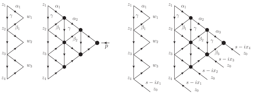
Figure 1: The diagrammatic representation for the layer operator $\Lambda_{N}(x_{1})$ and the eigenfunction $\Psi_{B}(p,\boldsymbol{x}|\boldsymbol{z})$ for $N=4$ (two left figures) and the layer operator $\widetilde{\Lambda}_{N}(x_{1})$ and the eigenfunction $\Psi_{A}(\boldsymbol{x}|\boldsymbol{z})$ for $N=4$ (two right figures). The line from $w$ to $z$ and the index $\alpha$ stands for the propagator, $[z-w]^{-\alpha}$, and the black dots – for the integration vertices. The indices have the following values: $\alpha_{k}=1-s-ix_{k}$, $\beta_{k}=1-s+ix_{k}$ and $\gamma=2s-1$. For the operator $\widetilde{\Lambda}$ and the eigenfunction $\Psi_{A}(\boldsymbol{x}|\boldsymbol{z})$ the variable $z_{0}=0$.

The functions $\Psi_{A}({\boldsymbol{x}}|\boldsymbol{z})$ and $\Psi_{B}(p\,,{\boldsymbol{x}}|\boldsymbol{z})$ being eigenfunctions of the self-adjoint operators form a complete orthogonal basis in the Hilbert space of the model

$$\int{d}^{2N}\boldsymbol{z}\,\overline{\Psi_{A}({\boldsymbol{x}^{\prime}}|\boldsymbol{z})}\,\Psi_{A}({\boldsymbol{x}}|\boldsymbol{z}) = \big{(}\boldsymbol{\mu}^{(A)}_{N}(\boldsymbol{x})\big{)}^{-1}\,\delta_{N}(\boldsymbol{x}-\boldsymbol{x}^{\prime})\,,$$ (27)

$$\int{d}^{2N}\boldsymbol{z}\,\overline{\Psi_{B}(p^{\prime}\,,{\boldsymbol{x}^{\prime}}|\boldsymbol{z})}\,\Psi_{B}(p\,,{\boldsymbol{x}}|\boldsymbol{z}) = \big{(}\boldsymbol{\mu}^{(B)}_{N}(\boldsymbol{x})\big{)}^{-1}\,\delta^{2}(\vec{p}-\vec{p}^{\prime})\,\delta_{N-1}(\boldsymbol{x}-\boldsymbol{x}^{\prime})\,.$$ (28)

Here $d^{2N}\!\boldsymbol{z}=d^{2}z_{1}\ldots d^{2}z_{N}$ and the delta function $\delta_{N}(\boldsymbol{x}-\boldsymbol{x}^{\prime})$ is defined as follows:

$$\delta_{N}(\boldsymbol{x}-\boldsymbol{x}^{\prime})=\frac{1}{N!}\sum_{s\in S_{N}}\delta^{(2)}(x_{1}-x^{\prime}_{s(1)})\cdots\delta^{(2)}(x_{N}-x^{\prime}_{s(N)})\,,$$ (29)

where the sum goes over all permutations of $N$ elements and

$$\delta^{(2)}(x-x^{\prime})\equiv\delta_{nn^{\prime}}\delta(\nu-\nu^{\prime}).$$ (30)

The weight functions $\boldsymbol{\mu}_{N}(\boldsymbol{x})$ and $\boldsymbol{\mu}_{N}(p,\boldsymbol{x})$ are the so-called Sklyanin’s measures. They were calculated in Refs. [7, 15] and take the following form

$$\boldsymbol{\mu}^{(A)}_{N}(\boldsymbol{x}) = \frac{1}{N!}\frac{\pi^{-N^{2}}}{(2\pi)^{N}}\prod_{k<j}[x_{k}-x_{j}]\,,$$ (31)

$$\boldsymbol{\mu}^{(B)}_{N}(\boldsymbol{x}) = \frac{1}{(N-1)!}\frac{2\pi^{-N^{2}}}{(2\pi)^{N}}\prod_{k<j}[x_{k}-x_{j}]\,.$$ (32)

The completeness condition for the functions $\Psi_{A}({\boldsymbol{x}}|\boldsymbol{z})$ and $\Psi_{B}({\boldsymbol{x}}\,,{\boldsymbol{p}}|\boldsymbol{z})$ reads

$$\prod_{k=1}^{N}\delta^{(2)}(\vec{z}_{k}-\vec{z}^{\prime}_{k}) = \int\mathcal{D}_{N}\boldsymbol{x}\,\boldsymbol{\mu}^{(A)}_{N}(\boldsymbol{x})\Psi_{A}({\boldsymbol{x}}|\boldsymbol{z})\,\overline{\Psi_{A}({\boldsymbol{x}}|\boldsymbol{z}^{\prime})}\,,$$ (33)

$$\prod_{k=1}^{N}\delta^{(2)}(\vec{z}_{k}-\vec{z}^{\prime}_{k}) = \int d^{2}p\,\int\mathcal{D}_{N-1}\boldsymbol{x}\,\boldsymbol{\mu}^{(B)}_{N}(\boldsymbol{x})\Psi_{B}({\boldsymbol{x}}\,,{\boldsymbol{p}}|\boldsymbol{z})\,\overline{\Psi_{B}({\boldsymbol{x}}\,,{\boldsymbol{p}}|\boldsymbol{z}^{\prime})}\,,$$ (34)

where the symbol $\mathcal{D}_{N}\boldsymbol{x}$ stands for

$$\int\mathcal{D}_{N}\boldsymbol{x}=\prod_{k=1}^{N}\left(\sum_{n_{k}=-\infty}^{\infty}\int_{-\infty}^{\infty}d\nu_{k}\right)\,$$ (35)

and the sum goes over all integers. The relations (33), (34) can be easily checked for $N=1,2$. The proof for general $N$ will be given elsewhere.

Let us note that for the case $N=1$ the eigenfunctions of the operators $B_{1}=-i\partial_{z}$ and $A_{1}(u)=u+i\big{(}s+z\partial_{z}\big{)}$ are the exponential and power functions, respectively. Namely,

$$\Psi_{B}(p|z)=e^{ipz+i\bar{p}\bar{z}}, \Psi_{A}(x|z)=[z]^{ix-s}\,.$$ (36)

The orthogonality and completeness relations for the power functions read

$$\int d^{2}z\,[z]^{ix_{1}-s}([z]^{ix_{2}-s})^{\ast} = \int d^{2}z\,[z]^{-1+i(x_{1}-x_{2})}=2\pi^{2}\delta^{(2)}(x_{1}-x_{2})\,,$$

$$\int Dx[z_{1}]^{ix-s}([z_{2}]^{ix-s})^{\ast} = {[z_{1}]^{-s}([z_{2}]^{-s})^{*}}\int Dx[z_{1}/z_{2}]^{ix}=2\pi^{2}\delta^{2}(\vec{z}_{1}-\vec{z}_{2})\,$$ (37)

and agree with (27), (33).

3 Matrix elements and integrals identities

Let us calculate the matrix element of the shift operator between the eigenstates of the operator $A_{N}$. We define

$$T_{z_{0}}(\boldsymbol{x},\boldsymbol{x}^{\prime})=\langle\Psi_{A}(\boldsymbol{x}^{\prime})|T_{z_{0}}|\Psi_{A}(\boldsymbol{x})\rangle\,.$$ (38)

The calculation of (38) goes along the following lines: first, using the representations (24) and (26) we write the matrix element as follows

$$\langle\Psi_{A}(\boldsymbol{x}^{\prime})|T_{z_{0}}|\Psi_{A}(\boldsymbol{x})\rangle=\widetilde{\Lambda}^{\dagger}_{1}(x^{\prime}_{N})\widetilde{\Lambda}_{2}^{\dagger}(x^{\prime}_{N-1})\cdots\widetilde{\Lambda}_{N}^{\dagger}(x^{\prime}_{1})\,\widetilde{\Lambda}_{N}^{(z_{0})}\left(x_{1}\right)\cdots\widetilde{\Lambda}_{2}^{(z_{0})}(x_{N-1})\,\widetilde{\Lambda}_{1}^{(z_{0})}(x_{N})\,.$$ (39)

Second, representing the product $\widetilde{\Lambda}_{N}^{\dagger}(x^{\prime}_{1})\,\widetilde{\Lambda}_{N}^{(z_{0})}(x_{1})$ as a Feynman diagram and simplifying it with the help of the identities (A.52), (A.53), (• ‣ A) in A one gets

$$\widetilde{\Lambda}_{N}^{\dagger}(x^{\prime})\,\widetilde{\Lambda}_{N}^{(z_{0})}(x)=[z_{0}]^{i(x-x^{\prime})}(-1)^{[s-ix]}\,q(x,x^{\prime})\,(Q^{(z_{0}=0)}_{N-1}(x))^{\dagger}Q^{(z_{0})}_{N-1}(x^{\prime})\,,$$ (40)

where the sign factor $(-1)^{[a]}\equiv(-1)^{a-\bar{a}}$ and the diagram for the operator $Q^{(z_{0})}_{N}(x)$ is shown in Fig. 2. The factor $q(x,x^{\prime})$ is given by the following expression

$$q(x,x^{\prime})=\pi a\big{(}1+i(x-x^{\prime})\big{)}\frac{a(\bar{s}-i\bar{x})}{a(s-ix^{\prime})}\,.$$ (41)

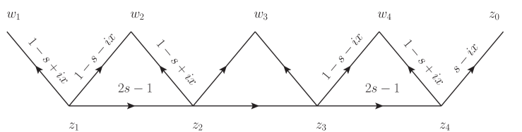
Figure 2: The diagrammatic representation for the operator $Q_{N}^{(z_{0})}(x)$ for $N=4$. Note that the index of the rightmost arrow differs from others.

Third, using the diagrammatic technique it is straightforward to check that

$$Q^{(z_{0})}_{k}(x^{\prime})\widetilde{\Lambda}_{k}^{(z_{0})}(x)=q(x,x^{\prime})\widetilde{\Lambda}_{k}^{(z_{0})}(x)Q^{(z_{0})}_{k-1}(x^{\prime})\,.$$ (42)

Thus one can reduce the $N$-point scalar product to the $N-1$-point product multiplied by some factor. It allows one immediately to get an answer for the matrix element (38)

$$T_{z_{0}}(\boldsymbol{x},\boldsymbol{x}^{\prime})=(-1)^{[A_{X}]}[z_{0}]^{i(X-X^{\prime})}\prod_{k,j=1}^{N}q(x_{k},x^{\prime}_{j})\,,$$ (43)

where we introduced the notations

$$X=\sum_{k}x_{k}, \bar{X}=\sum_{k}\bar{x}_{k}, A_{X}=\sum_{k}(s-ix_{k}), \bar{A}_{\bar{X}}=\sum_{k}(\bar{s}-i\bar{x}_{k}).$$

The calculation of the scalar product between the eigenfunctions of the operators $A_{N}$ and $B_{N}$ follows exactly the same lines so we give the final answer only

$$\langle\Psi_{B}(p,\boldsymbol{u})|\Psi_{A}(\boldsymbol{x})\rangle=i^{[A_{X}]}{\pi^{N}}{|p|^{-N-1}}[p]^{A_{X}}\prod_{k=1}^{N}a(\bar{s}-i\bar{x}_{k})\prod_{j=1}^{N-1}q(x_{k},u_{j})\,.$$ (44)

Note that the expressions (43) and (44) are symmetric functions of the separated variables as it should be. We also remark here that Eqs. (43), (44) have striking resemblance to the analogous expressions in the $SL(2,R)$ spin chain models, see Refs. [11, 12].

The function $a(1+i(x-x^{\prime}))$ entering (41) becomes singular for $x=x^{\prime}$. Indeed,

$$a(1+i(x-x^{\prime})) =\frac{\Gamma(i(\bar{x}^{\prime}-\bar{x}))}{\Gamma(1+i(x-x^{\prime}))}$$

$$=\frac{\Gamma(i(\nu^{\prime}-\nu)+(n-n^{\prime})/2)}{\Gamma(1-i(\nu^{\prime}-\nu)+(n-n^{\prime})/2)}=(-1)^{n-n^{\prime}}\frac{\Gamma(i(\nu^{\prime}-\nu)-(n-n^{\prime})/2)}{\Gamma(1-i(\nu^{\prime}-\nu)-(n-n^{\prime})/2)}\,.$$ (45)

Thus the function $a(1+i(x-x^{\prime}))$ is singular only when $n=n^{\prime}$ and $\nu=\nu^{\prime}$. The divergency comes from the chain integration and the right way to regularize it is to give the variable $\nu$ a small imaginary part, i.e. $x=-in/2+i\nu,\,\bar{x}=in/2+i\nu$ where $\text{Im}\,\nu>0$ (Note, that the variable $x$ is related to the function on the right side of the scalar product). So from now on we assume, whenever it is necessary, that the parameters $\nu_{k}$ in Eq. (18) have a positive imaginary part.

3.1 Gustafson integrals for $SL(2,\mathbb{C})$

In this section we present a generalization of the Gustafson’s integrals (Eq. 5.2 in Ref. [13]) to the complex case. Using the completeness condition (34) for the $B$–system one can represent the matrix element (38) in the form

$$T_{z_{0}}(\boldsymbol{x},\boldsymbol{x}^{\prime})=\int d^{2}p\,e^{-ipz_{0}-i\bar{p}\bar{z}_{0}}\int\mathcal{D}_{N-1}\boldsymbol{u}\,\boldsymbol{\mu}^{(B)}_{N}(\boldsymbol{u})\overline{\langle\Psi_{B}(p,\boldsymbol{u})|\Psi_{A}(\boldsymbol{x}^{\prime})\rangle}\langle\Psi_{B}(p,\boldsymbol{u})|\Psi_{A}(\boldsymbol{x})\rangle\,,$$ (46)

where we take into account that $T_{z_{0}}\Psi_{B}(p,{\boldsymbol{u}})=e^{-ipz_{0}-i\bar{p}\bar{z}_{0}}\Psi_{B}(p,{\boldsymbol{u}})$. Substituting the expressions (43) and (44) into (46) one gets after some algebra

$$\frac{1}{(N-1)!}\left(\prod_{k=1}^{N-1}\sum_{m_{k}=-\infty}^{\infty}\int_{-\infty}^{\infty}\frac{d\nu_{k}}{2\pi}\right)\frac{\prod_{k=1}^{N}\prod_{j=1}^{N-1}a(1+i(x_{k}-u_{j}))\,a(1+i(u_{j}-x^{\prime}_{k}))}{\prod_{m<j}a(1+i(u_{j}-u_{m}))a(1+i(u_{m}-u_{j}))}=\\ =\frac{\prod_{k,j=1}^{N}a(1+i(x_{k}-x^{\prime}_{j}))}{a(1+i(X-X^{\prime}))}\,.$$ (47)

We recall here that the integration variables $u_{k}$ take the values: $u_{k}=-{in_{k}}/2+\nu_{k},\ \ \bar{u}_{k}={in_{k}}/2+\nu_{k}$, where $n_{k}$ is an integer and $\nu_{k}$ is a real number. The external parameters $x_{k},x^{\prime}_{k}$ are

$$x_{k}=-\frac{im_{k}}{2}+\mu_{k}, \bar{x}_{k}=\frac{im_{k}}{2}+\mu_{k}, x^{\prime}_{k}=-\frac{im^{\prime}_{k}}{2}+\mu^{\prime}_{k}, \bar{x}_{k}=\frac{im^{\prime}_{k}}{2}+\mu^{\prime}_{k}\,,$$

where $m_{k},m^{\prime}_{k}$ are integers and $\mu_{k}$ and $\mu^{\prime}_{k}$ are complex numbers such that $\text{Im}\,\mu_{k}>0$ and $\text{Im}\,\mu^{\prime}_{k}<0$. It can be checked that for such a prescription the $\nu$-poles of the functions $a(1+i(x_{k}-u_{j}))$ and $a(1+i(u_{j}-x^{\prime}_{k}))$ are separated by the integration contour.

We also recall that the function $a(\alpha)\equiv a(\alpha,\bar{\alpha}))$, see Eq. (A.51), is a function of two complex variables such that $\alpha-\bar{\alpha}=n$. Namely, $a(\alpha)={\Gamma(1-\bar{\alpha})}/{\Gamma(\alpha)}$ and it is related to the gamma function for the complex field $\mathbb{C}$ defined in [16]

$$\Gamma(\alpha,\bar{\alpha})=i^{\alpha-\bar{\alpha}}\frac{\Gamma(\alpha)}{\Gamma(1-\bar{\alpha})}=i^{\alpha-\bar{\alpha}}a(1-\bar{\alpha})\,.$$ (48)

Thus, Eq. (47) is a direct analog of the first Gustafson’s integral (Eq. (5.2) in Ref. [13]) — the only difference consists in replacing the Euler gamma function by the function (48) and the corresponding modification of the integration measure. In was shown in [12] that many of Gustafson’s integrals can be obtained from the analysis of the matrix elements of the $SL(2,R)$ spin chain models. There is little doubt that such an analysis can be extended to the $SL(2,\mathbb{C})$ magnet and, therefore, it seem very plausible that many of Gustafson’s integrals admit an extension to the complex case.

Appendix A Diagram technique

This Appendix contains elements of the diagram technique which were used throughout the paper. The functions and kernels of operators are represented in the form of two-dimensional Feynman diagrams. The propagator is shown by the arrow directed from $w$ to $z$ with the index $\alpha$ attached to it

The propagator is given by the following expression

$$\frac{1}{[z-w]^{\alpha}}\equiv\frac{1}{(z-w)^{\alpha}(\bar{z}-\bar{w})^{\bar{\alpha}}}=\frac{(\bar{z}-\bar{w})^{\alpha-\bar{\alpha}}}{|z-w|^{2\alpha}}=\frac{(-1)^{\alpha-\bar{\alpha}}}{[w-z]^{\alpha}}\,,$$ (A.49)

where $\alpha-\bar{\alpha}=n_{\alpha}$ is integer. Performing the Fourier transform one defines the propagator in the momentum representation

$$\int d^{2}ze^{i(pz+\bar{p}\bar{z})}[z]^{-\alpha}=\pi\,i^{\alpha-\bar{\alpha}}\,a(\alpha)\,{[p]^{\alpha-1}}\,.$$ (A.50)

Here the notation $a(\alpha)$ is introduced for the function

$$a(\alpha)\equiv a(\alpha,\bar{\alpha})=\frac{\Gamma(1-\bar{\alpha})}{\Gamma(\alpha)}\,,\quad a(\bar{\alpha})=\frac{\Gamma(1-\alpha)}{\Gamma(\bar{\alpha})}\,,\quad a(\alpha,\beta,\gamma,\ldots)=a(\alpha)a(\beta)a(\gamma)\ldots$$ (A.51)

It has the following properties

$$a(\alpha)a(1-\bar{\alpha})=1\,,\quad a(1+\alpha)=-\frac{a(\alpha)}{\alpha\bar{\alpha}}\,,\quad a(\alpha)a(1-\alpha)=(-1)^{\alpha-\bar{\alpha}}\,,\quad a(\alpha)=(-1)^{\alpha-\bar{\alpha}}a(\bar{\alpha})\,.$$

The evaluation of Feynman diagrams is based on their transformation with the help of the certain rules

• Chain relation:

  $$\int d^{2}w\frac{1}{[z_{1}-w]^{\alpha}[w-z_{2}]^{\beta}}=(-1)^{\gamma-\bar{\gamma}}a(\alpha,\beta,\gamma)\frac{1}{[z_{1}-z_{2}]^{\alpha+\beta-1}}\,,$$ (A.52)

  where $\gamma=2-\alpha-\beta,\ \bar{\gamma}=2-\bar{\alpha}-\bar{\beta}$.

  

• Star– triangle relation:

  $$\int d^{2}w\frac{1}{[z_{1}-w]^{\alpha}[z_{2}-w]^{\beta}[z_{3}-w]^{\gamma}}=\frac{\pi a(\alpha,\beta,\gamma)}{[z_{2}-z_{1}]^{1-\gamma}[z_{1}-z_{3}]^{1-\beta}[z_{3}-z_{2}]^{1-\alpha}}\,,$$ (A.53)

  where $\alpha+\beta+\gamma=2$ and $\bar{\alpha}+\bar{\beta}+\bar{\gamma}=2$.

  

• Cross relation:

  $$\frac{1}{[z_{1}-z_{2}]^{\alpha^{\prime}-\alpha}}\int d^{2}w\frac{a(\alpha^{\prime},\bar{\beta}^{\prime})}{[w-z_{1}]^{\alpha}[w-z_{2}]^{1-\alpha^{\prime}}[w-z_{3}]^{\beta}[w-z_{4}]^{1-\beta^{\prime}}}=$$

  $$=\frac{1}{[z_{3}-z_{4}]^{\beta^{\prime}-\beta}}\int d^{2}\zeta\frac{a(\alpha,\bar{\beta})}{[w-z_{1}]^{\alpha^{\prime}}[w-z_{2}]^{1-\alpha}[w-z_{3}]^{\beta^{\prime}}[w-z_{4}]^{1-\beta}}\,,$$ (A.54)

  where $s-\bar{s}\in\mathbb{Z}$ and $\alpha+\beta=\alpha^{\prime}+\beta^{\prime}$.

  

Appendix B Mellin transform and star-triangle relation

In the simplest example $N=1$ (one site spin chain) the SoV-transformation related to the eigenfunctions of the $A$-operator coincides with the Mellin–Barnes transformation. In this Appendix we show that the star-triangle identity [18] is equivalent to the star-triangle relation (A.53) in the Mellin–Barnes representation.

Let $f(z,\bar{z})=f(r,\varphi)$ be a function on the complex plane. Combining the Fourier transform with respect to the angle variable $\varphi$ and the Mellin transform with respect to the radial variable $r$ one gets

$$f(z,\bar{z})=\sum_{n=-\infty}^{\infty}e^{i\varphi n}\int_{-\infty}^{\infty}d\nu\,r^{-2i\nu-1}f_{n}(\nu)=\int D\alpha\,[z]^{-1/2-\alpha}\hat{f}(\alpha),$$ (B.55)

where $\alpha=i\nu-n/2$, $\bar{\alpha}=i\nu+n/2\,\,$ and

$$\hat{f}(\alpha)\equiv f_{n}(\nu)=\frac{1}{2\pi^{2}}\int_{0}^{2\pi}d\varphi\,e^{-i\varphi n}\int_{0}^{\infty}dr\,r^{2i\nu-1}f(r,\varphi)=\frac{1}{2\pi^{2}}\int d^{2}z[z]^{-1/2+\alpha}\,f(z,\bar{z})\,.$$ (B.56)

These formulae are equivalent to the relations

$$\int d^{2}z\,[z]^{-1+\alpha}=2\pi^{2}\delta^{(2)}(\alpha)\,, \int D\alpha\,[z_{1}]^{-\alpha}[z_{2}]^{\alpha}=2\pi^{2}[z_{1}]\,\delta^{2}(\vec{z}_{1}-\vec{z}_{2})\,,$$ (B.57)

which are nothing else as the orthogonality and completeness relations (2.2). In order to avoid misunderstanding we recall that

$$\int D\alpha=\sum_{n\in\mathbb{Z}}\int_{-\infty}^{+\infty}\mathrm{d}\nu, \delta^{(2)}(\alpha-\alpha^{\prime})\equiv\delta_{nn^{\prime}}\delta(\nu-\nu^{\prime}).$$

Let us transform the start-triangle relation ($\beta_{1}+\beta_{2}+\beta_{3}=1$)

$$\int d^{2}w\frac{1}{[z_{1}-w]^{1-\beta_{1}}[z_{2}-w]^{1-\beta_{2}}[z_{3}-w]^{1-\beta_{3}}}=\frac{\pi a(1-\beta_{1}\,,1-\beta_{2}\,,1-\beta_{3})}{[z_{2}-z_{1}]^{\beta_{3}}[z_{1}-z_{3}]^{\beta_{2}}[z_{3}-z_{2}]^{\beta_{1}}}\,$$ (B.58)

to the Mellin–Barnes form. First of all, making use of the chain relation (A.52) we derive the following representation for the propagator

$$[w-z]^{\beta-1}=\frac{1}{2\pi}a(1-\beta)\int D\alpha\,\frac{a(1/2+\beta/2-\alpha)}{a(1/2-\beta/2-\alpha)}\,[z]^{-1/2+\beta/2-\alpha}\,[w]^{-1/2+\beta/2+\alpha}\,,$$ (B.59)

Next, multiplying both sides of Eq. (B.58) by the product $\prod_{i=1}^{3}[z_{i}]^{-1/2-\beta_{i}/2+\alpha_{i}}$ and integrating over all variables $z_{i}$ with the help of Eq. (B.57) we obtain

$$(2\pi^{2})\,\pi^{3}\,\delta^{(2)}\left(\sum\alpha_{i}\right)\prod_{i=1}^{3}a(1-\beta_{i})\frac{a\left(1/2+{\beta_{i}}/2-\alpha_{i}\right)}{a\left(1/2-{\beta_{i}}/2-\alpha_{i}\right)}=\\ =\pi^{4}\,\prod_{i=1}^{3}\int D\gamma_{i}\frac{a(1-\beta_{i}/2-\gamma_{i})}{a(\beta_{i}/2-\gamma_{i})}\delta^{(2)}(\gamma_{3}-\gamma_{2}-\alpha_{1})\delta^{(2)}(\gamma_{1}-\gamma_{3}-\alpha_{2})\delta^{(2)}(\gamma_{2}-\gamma_{1}-\alpha_{3})\,.$$ (B.60)

Comparing the coefficient at the delta function $\delta^{(2)}\left(\sum\alpha_{i}\right)$ on both sides we get

$$2\pi\prod_{i=1}^{3}a(1-\beta_{i})\frac{a\left(1/2+{\beta_{i}}/2-\lambda_{i,i+1}\right)}{a\left(1/2-{\beta_{i}}/2-\lambda_{i,i+1}\right)}=\int D\gamma\prod_{i=1}^{3}\frac{a(1-\beta_{i}/2-\gamma+\lambda_{i-1})}{a(\beta_{i}/2-\gamma+\lambda_{i-1})}\,,$$ (B.61)

where we put $\alpha_{i}=\lambda_{i}-\lambda_{i+1}$, $\gamma_{i}=-\lambda_{i-1}+\gamma$, $\lambda_{i+3}\equiv\lambda_{i}$. For the special choice of the parameters this relation is reduced to the to the star-triangle identity, Eq. (22) in Ref. [18].

References

References

• [1] E. K. Sklyanin, “Quantum inverse scattering method. Selected topics,” In: Quantum Group and Quantum Integrable Systems: Nankai Lectures on Mathematical Physics : Nankai Institute of Mathematics, China 2-18 April 1991 (World Scientific 1992), pp 63-97 [hep-th/9211111].
• [2] L. D. Faddeev, E. K. Sklyanin and L. A. Takhtajan, “The Quantum Inverse Problem Method. 1,” Theor. Math. Phys.  40 (1980) 688 [Teor. Mat. Fiz.  40 (1979) 194].
• [3] L. A. Takhtajan and L. D. Faddeev, “The Quantum method of the inverse problem and the Heisenberg XYZ model”, Russ. Math. Surveys 34 (1979) 11 [Usp. Mat. Nauk 34 (1979) 13].
• [4] P. P. Kulish and E. K. Sklyanin, “Quantum Spectral Transform Method. Recent Developments”, Lect. Notes Phys.  151 (1982) 61.
• [5] E. K. Sklyanin, “Separation of variables - new trends,” Prog. Theor. Phys. Suppl.  118 (1995) 35.
• [6] L. D. Faddeev, “How algebraic Bethe ansatz works for integrable model”, In: Quantum Symmetries/Symetries Quantiques, Proc.Les-Houches summer school, LXIV. Eds. A.Connes,K.Kawedzki, J.Zinn-Justin. North-Holland, 1998, 149-211, hep-th/9605187.
• [7] S. E. Derkachov, G. P. Korchemsky and A. N. Manashov, “Noncompact Heisenberg spin magnets from high-energy QCD: 1. Baxter Q operator and separation of variables,” Nucl. Phys. B 617 (2001) 375.
• [8] S. E. Derkachov, G. P. Korchemsky and A. N. Manashov, “Separation of variables for the quantum SL(2,R) spin chain,” JHEP 0307 (2003) 047.
• [9] S. E. Derkachov, G. P. Korchemsky and A. N. Manashov, “Baxter Q operator and separation of variables for the open SL(2,R) spin chain,” JHEP 0310 (2003) 053.
• [10] A. V. Silantyev, Transition function for the Toda chain, Theoretical and Mathematical Physics, Volume 150, 2007, Issue 3, pp.315-331
• [11] A. V. Belitsky, S. E. Derkachov and A. N. Manashov, Quantum mechanics of null polygonal Wilson loops, Nucl. Phys. B 882 (2014) 303 [arXiv:1401.7307 [hep-th]].
• [12] S. E. Derkachov and A. N. Manashov, Spin Chains and Gustafson’s Integrals, arXiv:1611.09593 [math-ph].
• [13] R. A. Gustafson, Some $q$-beta and Mellin–Barnes integrals on compact Lie groups and Lie algebras, Transactions of the American Mathematical Society Volume 341, Number 1, 1994.
• [14] R. A. Gustafson, Some $q$-beta and Mellin–Barnes integrals with many parameters associated to the classical groups, SIAM. J. Math. Anal., vol. 23, No. 3, 525, 1992.
• [15] S. E. Derkachov and A. N. Manashov, “Iterative construction of eigenfunctions of the monodromy matrix for $SL(2,\mathbb{C})$ magnet,” J. Phys. A 47 (2014) no.30, 305204, [arXiv:1401.7477 [math-ph]].
• [16] I. M. Gel’fand, M. I. Graev, V. S. Retakh, Hypergeometric functions over an arbitrary field, Russian Math. Surveys 59 (2004), no. 5, 831.
• [17] I. M. Gelfand, M. I. Graev and N. Ya. Vilenkin, Generalized functions, Vol. 5, Academic Press, 1966.
• [18] V. V. Bazhanov, V. V. Mangazeev and S. M. Sergeev, “Exact solution of the Faddeev-Volkov model,” Phys. Lett. A 372 (2008) 1547 [arXiv:0706.3077 [cond-mat.stat-mech]].