UWThPh-2016-27
CFTP/16-014
Charged-lepton decays from soft flavour violation

Abstract

We consider a two-Higgs-doublet extension of the Standard Model, with three right-handed neutrino singlets and the seesaw mechanism, wherein all the Yukawa-coupling matrices are lepton flavour-diagonal and lepton flavour violation is soft, originating solely in the non-flavour-diagonal Majorana mass matrix of the right-handed neutrinos. We consider the limit $m_{R}\to\infty$ of this model, where $m_{R}$ is the seesaw scale. We demonstrate that there is a region in parameter space where the branching ratios of all five charged-lepton decays $\ell_{1}^{-}\to\ell_{2}^{-}\ell_{3}^{+}\ell_{3}^{-}$ are close to their experimental upper bounds, while the radiative decays $\ell_{1}^{-}\to\ell_{2}^{-}\gamma$ are invisible because their branching ratios are suppressed by $m_{R}^{-4}$. We also consider the anomalous magnetic moment of the muon and show that in our model the contributions from the extra scalars, both charged and neutral, can remove the discrepancy between its experimental and theoretical values.

1 Introduction

In this paper we resume an old idea of two of us [1]: in a multi-Higgs-doublet model furnished with three right-handed neutrino singlets and the seesaw mechanism [2], lepton flavour may be conserved in the Yukawa couplings of all the Higgs doublets and violated solely in the Majorana mass terms of the right-handed neutrinos $\nu_{\ell R}$ ($\ell=e,\mu,\tau$), viz. in

$$\mathcal{L}_{\nu_{R}\,\mathrm{mass}}=-\frac{1}{2}\,\sum_{\ell_{1},\ell_{2}}\bar{\nu}_{\ell_{1}R}\left(M_{R}\right)_{\ell_{1}\ell_{2}}C\,\bar{\nu}_{\ell_{2}R}^{T}+{\rm H.c.},$$ (1)

where $C$ is the charge-conjugation matrix in Dirac space and $M_{R}$ is a non-singular symmetric matrix in flavour space. Since $\mathcal{L}_{\nu_{R}\,\mathrm{mass}}$ has dimension three, the violation of the individual lepton flavour numbers $L_{\ell}$ and of the total lepton number $L=L_{e}+L_{\mu}+L_{\tau}$ is soft. Thus, in our framework $\mathcal{L}_{\nu_{R}\,\mathrm{mass}}$ is responsible for

1. the smallness of the light-neutrino masses,

2. lepton mixing,

3. violation of $L$, and

4. violation of $L_{e}$, $L_{\mu}$, and $L_{\tau}$.

In this context, lepton flavour-violating processes were explicitly investigated at one-loop order in ref. [3] and the following property of our framework was discovered. Let $m_{R}$ denote the seesaw scale—the scale of the square roots of the eigenvalues of $M_{R}M_{R}^{\ast}$—and $n$ denote the number of Higgs doublets; it was found in ref. [3] that

1. the amplitudes of the lepton flavour-violating processes involving gauge bosons, like $\mu^{-}\to e^{-}\gamma$ and $Z^{0}\to e^{-}\mu^{+}$, scale down as $1\!\left/m_{R}^{2}\right.$ when $m_{R}\to\infty$; this holds even when in those processes the gauge bosons $\gamma$ and $Z^{0}$ are virtual, i.e. they are off-mass shell;

2. the amplitudes of the box diagrams for lepton flavour-violating processes like $\tau^{-}\to\mu^{-}\mu^{-}e^{+}$ and $\tau^{-}\to e^{-}e^{-}\mu^{+}$ also scale down as $1\!\left/m_{R}^{2}\right.$ for a large seesaw scale;

3. however, if $n\geq 2$, the amplitudes for lepton flavour-violating processes $\ell_{1}^{-}\to\ell_{2}^{-}\left(S^{0}_{b}\right)^{*}$, where $\left(S^{0}_{b}\right)^{\ast}$ is a virtual (off-mass shell) neutral scalar, approach a nonzero limit when $m_{R}\to\infty$. The non-decoupling of the seesaw scale in $\ell_{1}^{-}\to\ell_{2}^{-}\left(S^{0}_{b}\right)^{*}$ is an effect of the one-loop diagrams with neutrinos and charged scalars in the loop.

As a consequence, in our framework the amplitude of the process $\mu^{-}\to e^{-}e^{+}e^{-}$, which derives from $\mu^{-}\to e^{-}\left(S^{0}_{b}\right)^{*}$ followed by $\left(S^{0}_{b}\right)^{*}\to e^{+}e^{-}$, is unsuppressed in the limit $m_{R}\to\infty$. The same happens to the amplitudes of the four $\tau^{-}$ decays of the same type.

It is important to stress that in our model the amplitude for $\mu^{-}\to e^{-}e^{+}e^{-}$ is unsuppressed because of the penguin diagrams for neutral-scalar emission in the $\mu^{-}\to e^{-}$ conversion; indeed, the penguin diagrams for either $\gamma$ or $Z^{0}$ emission vanish in the limit $m_{R}\to\infty$. Thus, our model for lepton-flavour violation differs from, for instance, the scotogenic model discussed in ref. [4], wherein it is precisely the $\gamma$ and $Z^{0}$ penguins that are instrumental in $\mu^{-}\to e^{-}e^{+}e^{-}$ and in muon–electron conversion in nuclei.

Let us estimate a lower bound on $m_{R}$ by using the experimental bounds, given in table 1, on the radiative decays $\ell_{1}\to\ell_{2}\gamma$.

$\mbox{BR}\left(\mu^{+}\to e^{+}\gamma\right)$	$<$	$4.2\times 10^{-13}$
$\mbox{BR}\left(\tau^{-}\to e^{-}\gamma\right)$	$<$	$3.3\times 10^{-8}$
$\mbox{BR}\left(\tau^{-}\to\mu^{-}\gamma\right)$	$<$	$4.4\times 10^{-8}$
$\mbox{BR}\left(\mu^{-}\to e^{-}e^{+}e^{-}\right)$	$<$	$1.0\times 10^{-12}$
$\mbox{BR}\left(\tau^{-}\to e^{-}e^{+}e^{-}\right)$	$<$	$2.7\times 10^{-8}$
$\mbox{BR}\left(\tau^{-}\to e^{-}\mu^{+}\mu^{-}\right)$	$<$	$2.7\times 10^{-8}$
$\mbox{BR}\left(\tau^{-}\to\mu^{-}\mu^{+}\mu^{-}\right)$	$<$	$2.1\times 10^{-8}$
$\mbox{BR}\left(\tau^{-}\to\mu^{-}e^{+}e^{-}\right)$	$<$	$1.8\times 10^{-8}$

Table 1: The experimental bounds on the branching ratios of some lepton flavour-changing decays. All the bounds are at the 90% CL. The first bound is from ref. [5], all the other bounds are from ref. [6].

The amplitude for any such decay has the form

$$\mathcal{A}\left(\ell_{1}^{\pm}\to\ell_{2}^{\pm}\gamma\right)=e\,\varepsilon_{\rho}^{\ast}\,\bar{u}_{2}\left(i\sigma^{\rho\lambda}q_{\lambda}\right)\left(A_{L}\gamma_{L}+A_{R}\gamma_{R}\right)u_{1},$$ (2)

where $\varepsilon_{\rho}$ is the polarization vector of the photon, $u_{1}$ and $u_{2}$ are the spinors of $\ell_{1}^{\pm}$ and $\ell_{2}^{\pm}$, respectively, and $\gamma_{L}$ and $\gamma_{R}$ are the projectors of chirality. The decay rate is given, in the limit $m_{\ell_{2}}=0$, by

$$\Gamma\left(\ell_{1}^{\pm}\to\ell_{2}^{\pm}\gamma\right)=\frac{\alpha m_{\ell_{1}}^{3}}{4}\left(\left|A_{L}\right|^{2}+\left|A_{R}\right|^{2}\right).$$ (3)

Knowing that $A_{L}$ and $A_{R}$ are suppressed by $m_{R}^{-2}$, one may estimate, just on dimensional grounds, that

$$A_{L,R}\sim\frac{1}{16\pi^{2}}\,\frac{m_{\ell_{1}}}{m_{R}^{2}}.$$ (4)

Using the first two bounds of table 1 together with the experimental values for the masses and widths of the $\mu$ and $\tau$, one may then derive the lower bounds $m_{R}\gtrsim 50$ TeV from $\mu^{+}\to e^{+}\gamma$ and $m_{R}\gtrsim 2$ TeV from $\tau^{-}\to e^{-}\gamma$.

Thus, in the framework of ref. [3], if we take $m_{R}\gtrsim 500$ TeV then the radiative decays $\ell_{1}\to\ell_{2}\gamma$ are invisible in the foreseeable future. On the other hand, because of the nonzero limit of the amplitudes for $\ell_{1}\to\ell_{2}\left(S^{0}_{b}\right)^{*}$, the charged-lepton decays $\ell_{1}\to\ell_{2}\ell_{3}^{+}\ell_{3}^{-}$ are unsuppressed when $m_{R}\to\infty$. It is the purpose of this paper to investigate those decays numerically in the framework of ref. [3], assuming $m_{R}$ to be so large that the radiative charged-lepton decays are invisible. Then, $m_{R}$ is also much larger than the masses of the scalars in the model, which we assume to be in between one and a few TeV.

As a sideline, in this paper we also consider the contributions of both the neutral and charged scalars to the anomalous magnetic moment $a_{\ell}$ of the charged lepton $\ell$, with particular emphasis on $a_{\mu}$.

In order to keep the number of parameters of the model at a minimum, we restrict ourselves to just two Higgs doublets. Anticipating our results, we find that all five decays $\ell_{1}\to\ell_{2}\ell_{3}^{+}\ell_{3}^{-}$ may well be just around the corner, while at the same time the contributions of the non-Standard Model (SM) scalars of the model can make up for the discrepancy $a_{\mu}^{\mathrm{exp}}-a_{\mu}^{\mathrm{SM}}$ of the anomalous magnetic moment of the muon.

This paper is organized as follows. In section 2 we recall some results of ref. [3]. We then specialize to the case of just two Higgs doublets in section 3. We present the formulas for the contribution of the non-SM scalars to $a_{\ell}$ in section 4. Section 5 is devoted to a numerical simulation. In section 6 we summarize and conclude.

2 The lepton flavour-violating decays $\ell_{1}^{-}\to\ell_{2}^{-}\ell_{3}^{+}\ell_{3}^{-}$

2.1 The effective lepton flavour-violating interaction

The framework of ref. [3] assumes an $n$-Higgs-doublet setup wherein the violation of the family lepton numbers $L_{\ell}$ is soft. The corresponding Yukawa Lagrangian has the form

$${\cal L}_{\rm Yukawa}=-\sum_{k=1}^{n}\,\sum_{\ell=e,\mu,\tau}\left[\phi_{k}^{\dagger}\,\bar{\ell}_{R}\left(\Gamma_{k}\right)_{\ell\ell}+{\tilde{\phi}_{k}}^{\dagger}\,\bar{\nu}_{\ell R}\left(\Delta_{k}\right)_{\ell\ell}\right]D_{\ell L}+{\rm H.c.}$$ (5)

The basic assumption is

$$\mbox{the\ matrices}\ \Gamma_{k}\;\mbox{and}\ \Delta_{k}\;\mbox{are\ diagonal},\ \forall\;k=1,\ldots,n,$$ (6)

as is already implicit in equation (5). In that equation, the Higgs doublets and the left-handed-lepton gauge doublets are given by

$$\phi_{k}=\left(\begin{array}[]{c}\varphi_{k}^{+}\\[1.42262pt] \varphi_{k}^{0}\end{array}\right),\quad\tilde{\phi}_{k}=\left(\begin{array}[]{c}{\varphi_{k}^{0}}^{\ast}\\[1.42262pt] -\varphi_{k}^{-}\end{array}\right),\quad\mbox{and}\quad D_{\ell L}=\left(\begin{array}[]{c}\nu_{\ell L}\\[1.42262pt] \ell_{L}\end{array}\right),$$ (7)

respectively.

The scalar mass eigenfields $S_{a}^{+}$ and $S_{b}^{0}$ are related to the $\varphi_{k}^{+}$ and $\varphi^{0}_{k}$ by

$$\varphi_{k}^{+}=\sum_{a=1}^{n}U_{ka}S^{+}_{a}\quad\mbox{and}\quad\varphi_{k}^{0}=\frac{1}{\sqrt{2}}\left(v_{k}+\sum_{b=1}^{2n}V_{kb}S_{b}^{0}\right),$$ (8)

respectively [9]. The vacuum expectation values (VEVs) are $v_{k}\left/\sqrt{2}\right.$. The unitary $n\times n$ matrix $U$ diagonalizes the Hermitian mass matrix of the charged scalars. The $2n\times 2n$ real orthogonal matrix $\tilde{V}$, which diagonalizes the mass matrix of neutral scalar fields, is written as [9]

$$\tilde{V}=\left(\begin{array}[]{c}\mathrm{Re}\,V\\ \mathrm{Im}\,V\end{array}\right)\quad\mbox{with}\quad V\equiv\mathrm{Re}\,V+i\,\mathrm{Im}\,V.$$ (9)

The matrix $V$ is $n\times 2n$. We number the scalar mass eigenfields in such a way that $S_{1}^{\pm}=G^{\pm}$ and $S_{1}^{0}=G^{0}$ are the Goldstone bosons. If there is only one Higgs doublet, i.e. when $n=1$, the matrix $V$ is simply $V=\left(i,\ 1\right)$ in the phase convention where $v_{1}>0$, and $S^{0}_{2}$ is the Higgs field of the SM.

We define the diagonal matrices

$$M_{D}=\sum_{k=1}^{n}\frac{v_{k}}{\sqrt{2}}\,\Delta_{k},\quad M_{\ell}=\sum_{k=1}^{n}\frac{v_{k}^{\ast}}{\sqrt{2}}\,\Gamma_{k}=\mathrm{diag}\left(m_{e},m_{\mu},m_{\tau}\right).$$ (10)

According to ref. [3], in the limit $m_{R}\to\infty$, where $m_{R}$ is the seesaw scale, the flavour-changing interactions of the physical neutral scalars $S^{0}_{b}$, induced by loops with charged scalars and neutrinos, are given by

$$\mathcal{L}_{\mathrm{eff}}\left(S^{0}\right)=\sum_{b\geq 2}S^{0}_{b}\,\sum_{\ell_{1}\neq\ell_{2}}\bar{\ell}_{1}\left[\left(A_{L}^{b}\right)_{\ell_{1}\ell_{2}}\gamma_{L}+\left(A_{R}^{b}\right)_{\ell_{1}\ell_{2}}\gamma_{R}\right]\ell_{2}.$$ (11)

Note that the summation over $b$ begins with $b=2$, i.e. it excludes the Goldstone boson $S_{1}^{0}$. The coefficients $\left(A_{L,R}^{b}\right)_{\ell_{1}\ell_{2}}$ were computed in ref. [3]. Let us define the $3\times 3$ unitary matrix $U_{R}$ that diagonalizes $M_{R}$ as

$$U_{R}^{\dagger}M_{R}U_{R}^{*}=\mbox{diag}\left(m_{4},m_{5},m_{6}\right),$$ (12)

where $m_{4,5,6}$ are, in the limit $m_{R}\to\infty$, the masses of the heavy neutrinos. We next define

$$X_{\ell_{1}\ell_{2}}\equiv\frac{1}{16\sqrt{2}\pi^{2}}\,\sum_{i=4}^{6}\left[\left(U_{R}\right)_{\ell_{1}i}\left(U_{R}^{\ast}\right)_{\ell_{2}i}\ln{\frac{m_{i}^{2}}{\mu^{2}}}\right]=X_{\ell_{2}\ell_{1}}^{\ast},$$ (13)

where $\mu$ is a mass scale which is arbitrary because of the unitarity of $U_{R}$. Finally, we define the flavour space matrices $A_{1,2,3}$ as

$$\left(A_{1}\right)_{\ell_{1}\ell_{2}} \equiv \sum_{k=1}^{n}\left(\Gamma_{k}\right)_{\ell_{1}\ell_{1}}\left(\Delta_{k}\right)_{\ell_{2}\ell_{2}},$$ (14a)

$$\left(A_{2}\right)_{\ell_{1}\ell_{2}} \equiv \sum_{k=1}^{n}\left(\Delta_{k}^{\ast}\right)_{\ell_{1}\ell_{1}}\left(\Delta_{k}\right)_{\ell_{2}\ell_{2}},$$ (14b)

$$\left(A_{3}\right)_{\ell_{1}\ell_{2}} \equiv \sum_{k=1}^{n}\left(\Delta_{k}^{\ast}\right)_{\ell_{1}\ell_{1}}\left(\Gamma_{k}^{\ast}\right)_{\ell_{2}\ell_{2}}.$$ (14c)

Notice that $A_{3}=A_{1}^{\dagger}$ and $A_{2}=A_{2}^{\dagger}$. Then,

$$\left(A_{L}^{b}\right)_{\ell_{1}\ell_{2}}=\frac{X_{\ell_{1}\ell_{2}}A^{b}_{\ell_{1}\ell_{2}}}{m_{\ell_{1}}^{2}-m_{\ell_{2}}^{2}}\quad\mbox{and}\quad\left(A_{R}^{b}\right)_{\ell_{1}\ell_{2}}=\frac{X_{\ell_{2}\ell_{1}}^{\ast}\left(A^{b}_{\ell_{2}\ell_{1}}\right)^{\ast}}{m_{\ell_{2}}^{2}-m_{\ell_{1}}^{2}},$$ (15)

where $m_{\ell_{i}}$ is the mass of the charged lepton $\ell_{i}$ and

$$A^{b}_{\ell_{1}\ell_{2}} = \sum_{k=1}^{n}V_{kb}^{\ast}\left\{\left(\Delta_{k}^{\ast}\right)_{\ell_{1}\ell_{1}}\left(m_{\ell_{1}}^{2}-m_{\ell_{2}}^{2}\right)\left(A_{1}\right)_{\ell_{1}\ell_{2}}\right.$$

$$+\left(\Gamma_{k}\right)_{\ell_{1}\ell_{1}}\left[-m_{\ell_{1}}\left(M_{D}^{\ast}\right)_{\ell_{1}\ell_{1}}\left(A_{1}\right)_{\ell_{1}\ell_{2}}+\frac{m_{\ell_{2}}^{2}}{2}\,\left(A_{2}\right)_{\ell_{1}\ell_{2}}-m_{\ell_{2}}\left(M_{D}\right)_{\ell_{2}\ell_{2}}\left(A_{3}\right)_{\ell_{1}\ell_{2}}\right]$$

$$\left.+\left(\Gamma_{k}\right)_{\ell_{2}\ell_{2}}\left[m_{\ell_{2}}\left(M_{D}^{\ast}\right)_{\ell_{1}\ell_{1}}\left(A_{1}\right)_{\ell_{1}\ell_{2}}-\frac{m_{\ell_{1}}m_{\ell_{2}}}{2}\,\left(A_{2}\right)_{\ell_{1}\ell_{2}}+m_{\ell_{1}}\left(M_{D}\right)_{\ell_{2}\ell_{2}}\left(A_{3}\right)_{\ell_{1}\ell_{2}}\right]\right\}.$$

We note that, in every multi-Higgs-doublet model, it is possible to choose a basis for the scalar doublets such that only one of them, say $\phi_{1}$, has nonzero VEV:

$$\left\langle\varphi_{1}^{0}\right\rangle_{0}=\frac{v}{\sqrt{2}},\quad\left\langle\varphi_{k}^{0}\right\rangle_{0}=0\quad\forall\;k>1.$$ (17)

This basis is called the ‘Higgs basis’. In it, from equation (10),

$$\left(\Delta_{1}^{\ast}\right)_{\ell_{1}\ell_{1}}=\frac{\sqrt{2}}{v^{\ast}}\left(M_{D}^{\ast}\right)_{\ell_{1}\ell_{1}},\quad\left(\Gamma_{1}\right)_{\ell_{1}\ell_{1}}=\frac{\sqrt{2}}{v^{\ast}}\,m_{\ell_{1}}.$$ (18)

With equations (18) one finds that, in the sum over $k$ in equation (LABEL:AAAA), the term with $k=1$ gives a null contribution. Thus, in the Higgs basis, the contribution to $A^{b}_{\ell_{1}\ell_{2}}$ proportional to $V_{1b}^{\ast}$ is identically zero. In particular, if there is only one Higgs doublet, i.e. in the SM, $A^{b}_{\ell_{1}\ell_{2}}=0$, viz. when $n=1$ there are no effective lepton flavour-violating interactions of the neutral scalar in the limit $m_{R}\to\infty$.

2.2 The decay rate

If $\ell_{2}\neq\ell_{3}$, then $\ell_{1}^{-}\to\ell_{2}^{-}\ell_{3}^{+}\ell_{3}^{-}$ may be either $\tau^{-}\to\mu^{-}e^{+}e^{-}$ or $\tau^{-}\to e^{-}\mu^{+}\mu^{-}$. Equation (11) supplies the amplitude of the subprocess $\ell_{1}^{-}\to\ell_{2}^{-}\left(S^{0}_{b}\right)^{*}$. For the subsequent $\left(S^{0}_{b}\right)^{*}\to\ell_{3}^{+}\ell_{3}^{-}$ we have

$$\mathcal{L}^{(\ell^{\pm})}_{\mathrm{Yukawa}}\left(S^{0}\right)=-\frac{1}{\sqrt{2}}\,\sum_{b=2}^{2n}S^{0}_{b}\sum_{\ell=e,\mu\tau}\bar{\ell}\left[\left(\hat{\Gamma}_{b}\right)_{\ell\ell}\gamma_{L}+\left({\hat{\Gamma}}_{b}^{\dagger}\right)_{\ell\ell}\gamma_{R}\right]\ell,$$ (19)

where

$$\hat{\Gamma}_{b}\equiv\sum_{k=1}^{n}V_{kb}^{*}\Gamma_{k}.$$ (20)

We write the decay amplitude for $\ell_{1}^{-}\to\ell_{2}^{-}\ell_{3}^{+}\ell_{3}^{-}$ as

$$\mathcal{A}=\sum_{b=2}^{2n}\bar{u}_{2}\left[\left(\lambda_{b}\right)_{\ell_{2}\ell_{1}}\gamma_{L}+\left(\rho_{b}\right)_{\ell_{2}\ell_{1}}\gamma_{R}\right]u_{1}\,\bar{u}_{3}\left[\left(\hat{\Gamma}_{b}\right)_{\ell_{3}\ell_{3}}\gamma_{L}+\left(\hat{\Gamma}_{b}^{\dagger}\right)_{\ell_{3}\ell_{3}}\gamma_{R}\right]v_{3},$$ (21)

where, from equations (11) and (19),

$$\left(\lambda_{b}\right)_{\ell_{2}\ell_{1}}=-\frac{\left(A_{L}^{b}\right)_{\ell_{2}\ell_{1}}}{\sqrt{2}\,M_{b}^{2}}\quad\mbox{and}\quad\left(\rho_{b}\right)_{\ell_{2}\ell_{1}}=-\frac{\left(A_{R}^{b}\right)_{\ell_{2}\ell_{1}}}{\sqrt{2}\,M_{b}^{2}}.$$ (22)

In equations (22), $M_{b}$ is the mass of $S^{0}_{b}$. In the scalar propagators, we have neglected the four-momentum of the $\ell_{3}^{+}\ell_{3}^{-}$ subsystem. With the amplitude in equation (21), the decay rate is given by

$$\Gamma\left(\ell_{1}^{-}\to\ell_{2}^{-}\ell_{3}^{+}\ell_{3}^{-}\right) = \frac{m_{\ell_{1}}^{5}}{6144\pi^{3}}\left[\left|\sum_{b=2}^{2n}\left(\lambda_{b}\right)_{\ell_{2}\ell_{1}}\left({\hat{\Gamma}}_{b}\right)_{\ell_{3}\ell_{3}}\right|^{2}+\left|\sum_{b=2}^{2n}\left(\lambda_{b}\right)_{\ell_{2}\ell_{1}}\left({\hat{\Gamma}}_{b}^{\ast}\right)_{\ell_{3}\ell_{3}}\right|^{2}\right.$$ (23)

$$\left.+\left|\sum_{b=2}^{2n}\left(\rho_{b}\right)_{\ell_{2}\ell_{1}}\left({\hat{\Gamma}}_{b}\right)_{\ell_{3}\ell_{3}}\right|^{2}+\left|\sum_{b=2}^{2n}\left(\rho_{b}\right)_{\ell_{2}\ell_{1}}\left({\hat{\Gamma}}_{b}^{\ast}\right)_{\ell_{3}\ell_{3}}\right|^{2}\right].$$

We have neglected the masses of the final charged leptons in the kinematics.

If $\ell_{2}=\ell_{3}$, then $\ell_{1}^{-}\to\ell_{2}^{-}\ell_{2}^{+}\ell_{2}^{-}$ may be either $\mu^{-}\to e^{-}e^{+}e^{-}$ or $\tau^{-}\to e^{-}e^{+}e^{-}$ or $\tau^{-}\to\mu^{-}\mu^{+}\mu^{-}$. In equation (21) one must antisymmetrize the amplitude with respect to $\ell_{2}^{-}$ and in the kinematics one must insert an extra factor $1/2$. The final result is

$$\Gamma\left(\ell_{1}^{-}\to\ell_{2}^{-}\ell_{2}^{+}\ell_{2}^{-}\right) = \frac{m_{\ell_{1}}^{5}}{6144\pi^{3}}\left[\,\frac{1}{2}\,\left|\sum_{b=2}^{2n}\left(\lambda_{b}\right)_{\ell_{2}\ell_{1}}\left({\hat{\Gamma}}_{b}\right)_{\ell_{2}\ell_{2}}\right|^{2}+\frac{1}{2}\,\left|\sum_{b=2}^{2n}\left(\rho_{b}\right)_{\ell_{2}\ell_{1}}\left({\hat{\Gamma}}_{b}^{\ast}\right)_{\ell_{2}\ell_{2}}\right|^{2}\right.$$ (24)

$$\left.+\left|\sum_{b=2}^{2n}\left(\lambda_{b}\right)_{\ell_{2}\ell_{1}}\left({\hat{\Gamma}}_{b}^{\ast}\right)_{\ell_{2}\ell_{2}}\right|^{2}+\left|\sum_{b=2}^{2n}\left(\rho_{b}\right)_{\ell_{2}\ell_{1}}\left({\hat{\Gamma}}_{b}\right)_{\ell_{2}\ell_{2}}\right|^{2}\right].$$

3 Two Higgs doublets

From now on we assume $n=2$, i.e. a two-Higgs-doublet model. In the Higgs basis, the VEVs are given by

$$\left\langle\varphi_{1}^{0}\right\rangle_{0}=\frac{v}{\sqrt{2}},\quad\left\langle\varphi_{2}^{0}\right\rangle_{0}=0,$$ (25)

where $v\approx 246\,$GeV is real and positive. Thus, according to equation (8),

$$\varphi_{k}^{0}=\frac{1}{\sqrt{2}}\left(\delta_{k1}v+\sum_{b=1}^{4}V_{kb}S_{b}^{0}\right).$$ (26)

Moreover, the matrix $U$ is the $2\times 2$ unit matrix, i.e. $\varphi_{1}^{+}=S_{1}^{+}=G^{+}$ is the charged Goldstone boson and $\varphi_{2}^{+}=S_{2}^{+}$ is the physical charged scalar. According to the notation of ref. [9], the $4\times 4$ orthogonal matrix $\tilde{V}$ of equation (9), which diagonalizes the mass matrix of neutral scalar fields, is given by

$$\tilde{V}=\left(\begin{array}[]{cccc}0&R_{11}&R_{12}&R_{13}\\ 0&R_{21}&R_{22}&R_{23}\\ 1&0&0&0\\ 0&R_{31}&R_{32}&R_{33}\end{array}\right),\quad\textit{i.e.}\ V=\left(\begin{array}[]{cccc}i&R_{11}&R_{12}&R_{13}\\ 0&R_{21}+iR_{31}&R_{22}+iR_{32}&R_{23}+iR_{33}\end{array}\right),$$ (27)

with a $3\times 3$ orthogonal matrix $R$. The third row of $\tilde{V}$ corresponds to the neutral Goldstone boson $S_{1}^{0}=G^{0}$. The definition (20) reads

$$\hat{\Gamma}_{b}=\Gamma_{1}R_{1\,b-1}+\Gamma_{2}\left(R_{2\,b-1}-iR_{3\,b-1}\right)$$ (28)

for $b=2,3,4$. We parameterize the flavour-diagonal Yukawa coupling matrices as

$$\Gamma_{1} = \frac{\sqrt{2}}{v}\,\mbox{diag}\left(m_{e},m_{\mu},m_{\tau}\right)=\frac{\sqrt{2}}{v}\,M_{\ell},$$ (29a)

$$\Gamma_{2} = \mbox{diag}\left(\gamma_{e},\gamma_{\mu},\gamma_{\tau}\right),$$ (29b)

$$\Delta_{1} = \mbox{diag}\left(d_{e},d_{\mu},d_{\tau}\right)=\frac{\sqrt{2}}{v}\,M_{D},$$ (29c)

$$\Delta_{2} = \mbox{diag}\left(\delta_{e},\delta_{\mu},\delta_{\tau}\right).$$ (29d)

Therefore, from equations (14) and (LABEL:AAAA),

$$A^{b}_{\ell_{1}\ell_{2}} = V_{2b}^{\ast}\,A_{\ell_{1}\ell_{2}},$$ (30a)

$$A_{\ell_{1}\ell_{2}} = \frac{\sqrt{2}\left(m_{\ell_{1}}^{2}-m_{\ell_{2}}^{2}\right)m_{\ell_{1}}\delta_{\ell_{1}}^{*}d_{\ell_{2}}}{v}$$ (30b)

$$-\left(m_{\ell_{1}}^{2}+\frac{m_{\ell_{2}}^{2}}{2}\right)\gamma_{\ell_{1}}d_{\ell_{1}}^{*}d_{\ell_{2}}+\frac{3m_{\ell_{1}}m_{\ell_{2}}}{2}\,d_{\ell_{1}}^{*}\gamma_{\ell_{2}}d_{\ell_{2}}$$

$$+\left(m_{\ell_{1}}^{2}-\frac{m_{\ell_{2}}^{2}}{2}\right)\gamma_{\ell_{1}}\delta_{\ell_{1}}^{*}\delta_{\ell_{2}}-\frac{m_{\ell_{1}}m_{\ell_{2}}}{2}\,\delta_{\ell_{1}}^{*}\gamma_{\ell_{2}}\delta_{\ell_{2}}$$

$$+\frac{vm_{\ell_{2}}}{\sqrt{2}}\left(\gamma_{\ell_{1}}d_{\ell_{1}}^{*}\gamma_{\ell_{2}}\delta_{\ell_{2}}-\gamma_{\ell_{1}}\delta_{\ell_{1}}^{*}\gamma_{\ell_{2}}^{*}d_{\ell_{2}}\right)+\frac{vm_{\ell_{1}}}{\sqrt{2}}\left(\delta_{\ell_{1}}^{*}\left|\gamma_{\ell_{2}}\right|^{2}d_{\ell_{2}}-\gamma_{\ell_{1}}^{2}d_{\ell_{1}}^{*}\delta_{\ell_{2}}\right).\hskip 14.22636pt$$

As demonstrated at the end of section 2.1, in $A^{b}_{\ell_{1}\ell_{2}}$ the term proportional to $V_{1b}^{\ast}$ vanishes.

We now make the further assumption that $\phi_{1}$ is just identical with the Higgs doublet of the SM; this means that $S^{0}_{2}$ is exactly like the SM Higgs boson. This choice relieves us from having to take into account the experimental restrictions on the couplings of the SM Higgs boson, which become automatically fulfilled. We now have

$$\phi_{1}=\left(\begin{array}[]{c}S_{1}^{+}\\ \left(v+S_{2}^{0}+iS_{1}^{0}\right)\left/\sqrt{2}\right.\end{array}\right),$$ (31)

where $S_{1}^{+}=G^{+}$ and $S_{1}^{0}=G^{0}$ are the Goldstone bosons. This means that we choose $R_{11}=1$, whence it follows that $R$ can be written as

$$R=\left(\begin{array}[]{ccc}1&0&0\\ 0&\cos{\alpha}&\sin{\alpha}\\ 0&-\sin{\alpha}&\cos{\alpha}\end{array}\right).$$ (32)

The matrix $V$ is

$$V=\left(\begin{array}[]{cccc}i&1&0&0\\ 0&0&e^{-i\alpha}&ie^{-i\alpha}\end{array}\right).$$ (33)

Thus, from equation (26),

$$\phi_{2}=\left(\begin{array}[]{c}S_{2}^{+}\\ e^{-i\alpha}\left(S_{3}^{0}+iS_{4}^{0}\right)\left/\sqrt{2}\right.\end{array}\right).$$ (34)

From equation (28),

$$\hat{\Gamma}_{2}=\Gamma_{1},\quad\hat{\Gamma}_{3}=e^{i\alpha}\Gamma_{2},\quad\hat{\Gamma}_{4}=-ie^{i\alpha}\Gamma_{2},$$ (35)

and, from equation (30a),

$$A^{2}_{\ell_{1}\ell_{2}}=0,\quad A^{3}_{\ell_{1}\ell_{2}}=e^{i\alpha}A_{\ell_{1}\ell_{2}},\quad A^{4}_{\ell_{1}\ell_{2}}=-ie^{i\alpha}A_{\ell_{1}\ell_{2}}.$$ (36)

The decay rates are then

$$\Gamma\left(\ell_{1}^{-}\to\ell_{2}^{-}\ell_{3}^{+}\ell_{3}^{-}\right) = \frac{m_{\ell_{1}}^{5}}{6144\pi^{3}}\left|X_{\ell_{2}\ell_{1}}\right|^{2}\left|\gamma_{\ell_{3}}\right|^{2}\frac{\left|A_{\ell_{2}\ell_{1}}\right|^{2}+\left|A_{\ell_{1}\ell_{2}}\right|^{2}}{\left(m_{\ell_{2}}^{2}-m_{\ell_{1}}^{2}\right)^{2}}\left(\frac{1}{M_{3}^{4}}+\frac{1}{M_{4}^{4}}\right),$$ (37a)

$$\Gamma\left(\ell_{1}^{-}\to\ell_{2}^{-}\ell_{2}^{+}\ell_{2}^{-}\right) = \frac{m_{\ell_{1}}^{5}}{6144\pi^{3}}\left|X_{\ell_{2}\ell_{1}}\right|^{2}\left|\gamma_{\ell_{2}}\right|^{2}\frac{\left|A_{\ell_{2}\ell_{1}}\right|^{2}+\left|A_{\ell_{1}\ell_{2}}\right|^{2}}{\left(m_{\ell_{2}}^{2}-m_{\ell_{1}}^{2}\right)^{2}}$$ (37b)

$$\hskip 110.96574pt\times\left[\frac{3}{4}\left(\frac{1}{M_{3}^{4}}+\frac{1}{M_{4}^{4}}\right)+\frac{1}{2M_{3}^{2}M_{4}^{2}}\right].\hskip 22.76219pt$$

The decay rates depend on the masses $M_{3}$ and $M_{4}$ of the non-SM neutral scalar fields $S^{0}_{3}$ and $S^{0}_{4}$, respectively. There is no dependence on the phase $\alpha$. In equation (37a), $\ell_{2}\neq\ell_{3}$ is understood.

4 The anomalous magnetic moment of the muon

Let $a_{\ell}^{(S)}$ denote the contributions of the non-SM scalars $S^{0}_{3}$, $S^{0}_{4}$, and $S^{\pm}_{2}$ to the anomalous magnetic moment (AMM) of the charged lepton $\ell$. To a good approximation,

$$a_{\ell}^{(S)} \simeq \frac{m_{\ell}^{2}}{96\pi^{2}}\left\{2\left|\gamma_{\ell}\right|^{2}\left(\frac{1}{M_{3}^{2}}+\frac{1}{M_{4}^{2}}\right)\right.$$ (38c)

$$-3\,\mbox{Re}\left(e^{2i\alpha}\gamma_{\ell}^{2}\right)\left[\frac{1}{M_{3}^{2}}\left(3+2\ln\frac{m_{\ell}^{2}}{M_{3}^{2}}\right)-\frac{1}{M_{4}^{2}}\left(3+2\ln\frac{m_{\ell}^{2}}{M_{4}^{2}}\right)\right]$$

$$\left.-\frac{\left|\gamma_{\ell}\right|^{2}}{\mu_{2}^{2}}\right\}.$$

Lines (38c) and (38c) derive from a loop with $\ell$ and either $S_{3}^{0}$ or $S_{4}^{0}$; the photon line attaches to $\ell$. Line (38c) comes from a loop with $S_{2}^{\pm}$ and light neutrinos, wherein the external photon attaches to $S_{2}^{\pm}$; in that line, $\mu_{2}$ denotes the mass of $S^{\pm}_{2}$. We have dropped all the terms proportional to $m_{R}^{-2}$, including in particular the contributions from the loop with $S_{2}^{\pm}$ and heavy neutrinos. For the coupling of the charged scalars to the charged leptons we refer the reader to ref. [3].

There is a long-standing discrepancy between the experimental value of the AMM of the muon, $a_{\mu}^{\mathrm{exp}}$, and the SM theoretical value of that AMM, $a_{\mu}^{\mathrm{SM}}$ [10]:

$$a_{\mu}^{\mathrm{exp}}-a_{\mu}^{\mathrm{SM}}=\left\{\begin{array}[]{l}(287\pm 80)\times 10^{-11}\ (\mbox{at}\ 3.6\,\sigma)~{}\cite[cite]{[\@@bibref{}{davier}{}{}]},\\ (261\pm 78)\times 10^{-11}\ (\mbox{at}\ 3.3\,\sigma)~{}\cite[cite]{[\@@bibref{}{hagiwara}{}{}]}.\end{array}\right.$$ (39)

If this discrepancy signals new physics, then the contributions of the scalars in our model to the AMM of the muon may be relevant. Taking for instance $\gamma_{\mu}^{2}$ real and $e^{2i\alpha}=1$, one has

$$a_{\mu}^{(S)}\simeq-\frac{\gamma_{\mu}^{2}}{96\pi^{2}}\left[\frac{m_{\mu}^{2}}{M_{3}^{2}}\left(7+6\ln\frac{m_{\mu}^{2}}{M_{3}^{2}}\right)-\frac{m_{\mu}^{2}}{M_{4}^{2}}\left(11+6\ln\frac{m_{\mu}^{2}}{M_{4}^{2}}\right)+\frac{m_{\mu}^{2}}{\mu_{2}^{2}}\right].$$ (40)

The right-hand side of equation (40) is dominated by the two terms with logarithms. One readily sees that the terms with $M_{4}$ and $\mu_{2}$ give negative contributions to $a_{\mu}^{(S)}$ (assuming $\gamma_{\mu}^{2}$ to be positive), while the term with $M_{3}$ gives a positive contribution; since $a_{\mu}^{\mathrm{exp}}-a_{\mu}^{\mathrm{SM}}$ is positive, we would like the term with $M_{3}$ to dominate over the other two; this is achieved with $M_{3}<M_{4}$. Taking for instance $M_{3}=1\,$TeV, $M_{4}=\mu_{2}=2$ TeV, and $\gamma_{\mu}=1.7$, we find $a_{\mu}^{(S)}=258\times 10^{-11}$, which is of the right sign and absolute value to explain the discrepancy (39). We conclude that our model can, using reasonable parameters, fill the gap between $a_{\mu}^{\mathrm{exp}}$ and $a_{\mu}^{\mathrm{SM}}$.

The experimental AMM of the electron is in good agreement with the SM prediction for $a_{e}$. We must therefore check that the non-SM scalars of our model give an $a_{e}^{(S)}$ smaller than the experimental error $2.6\times 10^{-13}$ [6] of $a_{e}$. We might of course simply take $\gamma_{e}=0$, but this would eliminate e.g. the decay $\mu^{-}\to e^{-}e^{+}e^{-}$, which we would like to have close to its experimental upper limit. So we use instead the same scalar masses as before and choose $\gamma_{e}=1.7$, obtaining $a_{e}^{(S)}=1.0\times 10^{-13}$. Thus, even for a relatively large $\gamma_{e}$, $a_{e}^{(S)}$ can be below the experimental error. This is of course because of the tiny electron mass.

5 Numerics

In this section, we want to show that in the two-Higgs-doublet version of the framework of ref. [3], and assuming moreover $R_{11}=1$, there is a region in parameter space where the branching ratios of all five decays $\ell_{1}^{-}\to\ell_{2}^{-}\ell_{3}^{+}\ell_{3}^{-}$ are close to their present experimental upper bounds displayed in table 1.

Notice that we only strive in this section to prove that something is possible; we do not attempt a full scan of the parameter space of our model, which is quite vast. On the contrary, we shall make many simplifying assumptions, for instance we assume that all the parameters of the model are real.

In the decay rates of equations (37) there are various unknowns:

1. the neutral-scalar masses $M_{3}$ and $M_{4}$;

2. the factors $\left|X_{\ell_{2}\ell_{1}}\right|^{2}$;

3. the Yukawa couplings $\gamma_{\ell}$ together with those in $A_{\ell\ell^{\prime}}$.

In this section we also want to fit $a_{\mu}^{\mathrm{exp}}-a_{\mu}^{\mathrm{SM}}$ of equation (39) by using $a_{\mu}^{(S)}$ of equation (38); in that equation there are the neutral-scalar masses $M_{3}$ and $M_{4}$, the charged-scalar mass $\mu_{2}$, the Yukawa coupling $\gamma_{\mu}$, and the phase $\alpha$. In order to simplify our task, we fix all those parameters at the values used in section 4, viz.

$$M_{3}=1\,\mathrm{TeV},\quad M_{4}=2\,\mathrm{TeV},$$ (41a)

$$\gamma_{\mu}=1.7.$$ (41b)

Thus, the neutral-scalar masses mentioned in point 1 above are fixed through equation (41a). Notice in equation (41b) that $\gamma_{\mu}$ is assumed to be real.

In order to compute the factors $\left|X_{\ell_{2}\ell_{1}}\right|^{2}$ we proceed in the following way. The mass matrix of the light neutrinos is obtained by the seesaw formula. In our notation, it reads

$$\mathcal{M}_{\nu}=-M_{D}^{T}M_{R}^{-1}M_{D}=-\frac{v^{2}}{2}\,\Delta_{1}M_{R}^{-1}\Delta_{1},$$ (42)

where $\Delta_{1}=\mathrm{diag}\left(d_{e},d_{\mu},d_{\tau}\right)$ is diagonal. We shall fix

$$d_{e}=0.6,\quad d_{\mu}=d_{\tau}=0.1.$$ (43)

Inverting equation (42), we obtain

$$M_{R}=-\frac{v^{2}}{2}\,\Delta_{1}\mathcal{M}_{\nu}^{-1}\Delta_{1}.$$ (44)

The matrix $\mathcal{M}_{\nu}$ is diagonalized as

$$V_{L}^{T}\mathcal{M}_{\nu}V_{L}=\mbox{diag}\left(m_{1},m_{2},m_{3}\right)\equiv\hat{m},$$ (45)

where $m_{1,2,3}$ are the light-neutrino masses and $V_{L}=e^{i\hat{\alpha}}\,U_{\mathrm{PMNS}}\,e^{i\hat{\beta}}$ is identical to the lepton mixing matrix $U_{\mathrm{PMNS}}$, apart from a diagonal matrix of unphysical phases $e^{i\hat{\alpha}}$ on the left and apart from the Majorana phase factors of the diagonal matrix $e^{i\hat{\beta}}$ on the right. Using equations (44) and (45) together with the fact that the matrices $\Delta_{1}$, $\hat{m}$, $e^{i\hat{\alpha}}$, and $e^{i\hat{\beta}}$ are diagonal, we obtain

$$M_{R}=-\frac{v^{2}}{2}\,e^{i\hat{\alpha}}\Delta_{1}\,U_{\mathrm{PMNS}}\left(e^{2i\hat{\beta}}\hat{m}^{-1}\right)U_{\mathrm{PMNS}}^{T}\,\Delta_{1}e^{i\hat{\alpha}}.$$ (46)

Using our simplifying assumption that all the parameters in the model are real, we set in equation (46) $e^{i\hat{\alpha}}=e^{i\hat{\beta}}=\mathbbm{1}$ and we also assume that $U_{\mathrm{PMNS}}$ is real. Using the standard parameterization for $U_{\mathrm{PMNS}}$ in ref. [6], we fix $e^{i\delta}=-1$; we also fix the mixing angles at their best-fit values of ref. [15], viz. $s_{12}^{2}=0.304$, $s_{23}^{2}=0.452$, and $s_{13}^{2}=0.0218$. We also have to choose the type of light-neutrino mass spectrum, either normal or inverted—for definiteness, we settle on a normal mass spectrum. Let the lightest neutrino mass $m_{1}$, which is unknown to date, be a free parameter; with a choice for $m_{1}$ and the best-fit values $\Delta m^{2}_{21}=7.50\times 10^{-5}\,\mathrm{eV}^{2}$ and $\Delta m^{2}_{31}=2.457\times 10^{-3}\,\mathrm{eV}^{2}$ of ref. [15], we obtain for the other two light-neutrino masses

$$m_{2}=\sqrt{m_{1}^{2}+\Delta m^{2}_{21}}\quad\mbox{and}\quad m_{3}=\sqrt{m_{1}^{2}+\Delta m^{2}_{31}}.$$ (47)

We are now able to compute the matrix $M_{R}$ as a function of $m_{1}$ through equation (46); therefrom we compute the quantities $\left|X_{\ell_{2}\ell_{1}}\right|^{2}$ by using equations (12) and (13). We obtain the result depicted in figure 1.

Figure 1: The factors $\left|X_{\ell_{2}\ell_{1}}\right|^{2}$ as functions of $m_{1}$. The full line gives $\left|X_{e\mu}\right|^{2}$, the dashed line gives $\left|X_{e\tau}\right|^{2}$, and the dashed-dotted line is $\left|X_{\mu\tau}\right|^{2}$.

Notice that $X_{e\mu}$ has a zero for $m_{1}\approx 0.0086$ eV; else, the $\left|X_{\ell_{2}\ell_{1}}\right|^{2}$ are decreasing functions of $m_{1}$, and vary by a few orders of magnitude from $m_{1}=0$ to $m_{1}=0.1\,$eV. From now one we fix

$$m_{1}=0.05\,\mbox{eV}.$$ (48)

We then have

$$\left|X_{e\mu}\right|^{2}=1.99\times 10^{-8},\quad\left|X_{e\tau}\right|^{2}=4.43\times 10^{-8},\quad\left|X_{\mu\tau}\right|^{2}=2.11\times 10^{-6}.$$ (49)

In this way we have fixed the factors mentioned in point 2 above. Besides equations (49), we also obtain, from equation (48), heavy-neutrino masses $m_{4}=4.3\times 10^{12}$ GeV, $m_{5}=6.0\times 10^{12}$ GeV, and $m_{6}=2.2\times 10^{14}$ GeV. These masses represent the seesaw scale, which is so large that all the radiative charged-lepton decays are completely invisible. Actually, $m_{R}$ is this large partly because we chose the Yukawa couplings $d_{\ell}$ close to one, cf. equation (43), in order to achieve large $\tau$-lepton branching ratios. Thus, the effect that we want to produce in our model can only occur for a large seesaw scale—it disappears, at least in the case of the $\tau$-lepton, for small $m_{R}$.

Some of the Yukawa couplings mentioned in point 3 are given in equations (41) and (43). We now fix the remaining Yukawa couplings as

$$\gamma_{e}=\gamma_{\tau}=1.7,\quad\delta_{e}=0,\quad\delta_{\mu}=0.00007,\quad\delta_{\tau}=0.2.$$ (50)

With all these input values, we obtain the branching ratios

$$\mathrm{BR}\left(\mu^{-}\to e^{-}e^{+}e^{-}\right) = 3.872\times 10^{-13},$$ (51a)

$$\mathrm{BR}\left(\tau^{-}\to e^{-}e^{+}e^{-}\right) = 1.111\times 10^{-8},$$ (51b)

$$\mathrm{BR}\left(\tau^{-}\to e^{-}\mu^{+}\mu^{-}\right) = 1.280\times 10^{-8},$$ (51c)

$$\mathrm{BR}\left(\tau^{-}\to\mu^{-}\mu^{+}\mu^{-}\right) = 1.307\times 10^{-8},$$ (51d)

$$\mathrm{BR}\left(\tau^{-}\to\mu^{-}e^{+}e^{-}\right) = 1.506\times 10^{-8}.$$ (51e)

One sees that all these branching ratios are less than a factor of three away from the upper bounds of table 1. We have thus demonstrated that in our model it is possible to suppress the radiative decays of the muon and tau lepton, while keeping the branching ratios of their decays into charged leptons very close to the experimental upper bounds.

Some remarks concerning the input values that we have utilized are in order:

• All the experimental upper bounds on the branching ratios of the decays of the $\tau$-lepton in table 1 are quite similar. Therefore, if we want to have both $\tau^{-}\to\ell^{-}e^{+}e^{-}$ and $\tau^{-}\to\ell^{-}\mu^{+}\mu^{-}$ close to their experimental upper bounds, then $\gamma_{e}$ and $\gamma_{\mu}$ will have to be similar—see the explicit factors $\gamma_{\ell_{3}}$ and $\gamma_{\ell_{2}}$ in the decay rates of equations (37a) and (37b), respectively. For definiteness we have chosen all three $\gamma_{\ell}$ to be the same. In figure 2 we depict the way the five branching ratios vary as functions of some $\gamma_{\ell}$.

  

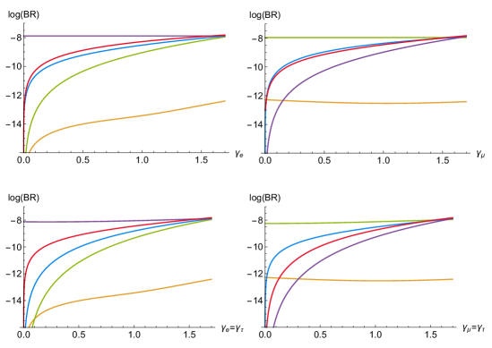
  Figure 2: $\mathrm{BR}\left(\mu^{-}\to e^{-}e^{+}e^{-}\right)$ (orange line), $\mathrm{BR}\left(\tau^{-}\to e^{-}e^{+}e^{-}\right)$ (green line), $\mathrm{BR}\left(\tau^{-}\to e^{-}\mu^{+}\mu^{-}\right)$ (blue line), $\mathrm{BR}\left(\tau^{-}\to\mu^{-}\mu^{+}\mu^{-}\right)$ (lilac line), and $\mathrm{BR}\left(\tau^{-}\to\mu^{-}e^{+}e^{-}\right)$ (red line) as functions of various Yukawa couplings. In the top-left figure, $\gamma_{e}$ varies in between 0 and 1.7. In the top-right figure, $\gamma_{\mu}$ varies. Bottom left, $\gamma_{e}$ and $\gamma_{\tau}$ change but with $\gamma_{\tau}$ remaining equal to $\gamma_{e}$. In the bottom right, $\gamma_{\mu}=\gamma_{\tau}$ varies. In all the figures, all the Yukawa couplings that do not vary take the values in equations (41b), (43), and (50).

• In $A_{\ell_{1}\ell_{2}}$ in equation (30b) the dominant terms have $v\simeq 246$ GeV in the numerator. For large $\gamma_{e}=\gamma_{\mu}=1.7$ and large $d_{e}=0.6$ and $d_{\mu}=0.1$, these terms will give a much too large contribution to $\mbox{BR}\left(\mu^{-}\to e^{-}e^{+}e^{-}\right)$ unless there is a delicate cancellation between the terms proportional to $\delta_{e}$ and the terms proportional to $\delta_{\mu}$. This cancellation is illustrated in figure 3 for $\delta_{\mu}$ of equation (50). For larger values of $\delta_{\mu}$ the curve is basically identical but shifted to the right.

  

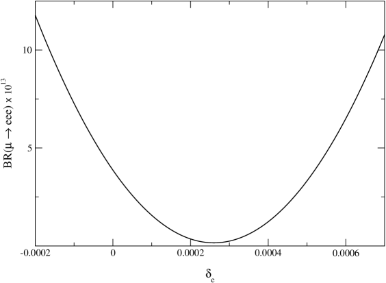
  Figure 3: $\mathrm{BR}\left(\mu^{-}\to e^{-}e^{+}e^{-}\right)$ as a function of the Yukawa coupling $\delta_{e}$ while all the other Yukawa couplings remain fixed at their values in equations (41b), (43), and (50). The experimental bound $\mathrm{BR}\left(\mu^{-}\to e^{-}e^{+}e^{-}\right)\times 10^{13}<10$ is not depicted in this figure but must be taken into account.

• On the other hand, in the decays of the $\tau$-lepton the terms with $v$ in the numerator are just the relevant ones and we have needed, since we have chosen tiny $\delta_{e}$ and $\delta_{\mu}$, large parameters $\delta_{\tau}$, $d_{e}$, $d_{\mu}$, and $\gamma_{\ell}$ ($\ell=e,\mu,\tau$).

We may thus say that the branching ratios in equations (51) involve some finetuning.

6 Conclusions

It is now known, since the experimental observation of neutrino oscillations [16], that there is lepton flavour-violation. However, that violation has not yet been observed in the charged-lepton sector and it is not quite certain where it is most likely to be observed first. In this context, the radiative decays $\ell_{1}^{\pm}\to\ell_{2}^{\pm}\gamma$ seem the best guess, and decays of the form $\ell_{1}^{\pm}\to\ell_{2}^{\pm}\ell_{3}^{+}\ell_{3}^{-}$ may be an option as well.

In this paper we have demonstrated, through an explicit numerical example, that there is a class of models where the radiative decays in the paragraph above may be so suppressed as to be utterly invisible, yet any of the five decays of the form $\ell_{1}^{\pm}\to\ell_{2}^{\pm}\ell_{3}^{+}\ell_{3}^{-}$, or indeed—if one assumes some finetuning—all such five decays simultaneously, may be just around the corner.

Our class of models, first considered in ref. [1], has three right-handed neutrino singlets and has more than one Higgs doublet. The crucial assumption is that the lepton flavours are conserved in the Yukawa couplings and broken only in the Majorana mass terms of the right-handed neutrinos; this assumption is field-theoretically consistent because those mass terms have dimension three while the Yukawa couplings have dimension four. As demonstrated in ref. [3], the effect mentioned in the previous paragraph occurs if the seesaw scale is much larger than all other scales in this class of models. In the present paper we have shown that there is a relevant simplification of the effective flavour-violating couplings of the neutral scalars, emerging at the one-loop level, when one uses the Higgs basis, i.e. the basis for the Higgs doublets wherein only one of them has nonzero VEV.

We have explicitly computed the branching ratios of the five decays $\ell_{1}^{\pm}\to\ell_{2}^{\pm}\ell_{3}^{+}\ell_{3}^{-}$ in the case of a two-Higgs-doublet model assuming that the first doublet $\phi_{1}$ coincides with the Higgs doublet of the SM, viz. it does not mix with the second doublet. Moreover, we have employed several simplifying assumptions in order to reduce the parameter space of the model. We have noted that some finetuning is needed in order that $\mathrm{BR}\left(\mu^{-}\to e^{-}e^{+}e^{-}\right)$ does not become too large when all other four branching ratios are simultaneously close to their experimental limits.

Flavour-diagonal Yukawa coupling matrices have no straightforward implementation in the quark sector, so one has to admit non-diagonal Yukawa couplings there and avoid excessive flavour-changing neutral interactions by finetuning. Thus there is an asymmetry between the quark and the lepton sector. This may seem ugly, but, as pointed out in this paper, the intriguing consequences for charged-lepton decays make a consideration of such a framework worthwhile.

Acknowledgements:

E.H.A. is supported by the FWF Austrian Science Fund under the Doctoral Program W1252-N27 “Particles and Interactions.” L.L. is supported by the FCT Portuguese Science Foundation through the projects CERN/FIS-NUC/0010/2015 and UID/FIS/00777/2013, which are partially funded by POCTI (FEDER), COMPETE, QREN, and the European Union.

References

-
[1]
L. Lavoura and W. Grimus,
Seesaw model with softly broken ,
JHEP 0009 (2000) 007
[hep-ph/0008020];
W. Grimus and L. Lavoura, Softly broken lepton numbers and maximal neutrino mixing, JHEP 0107 (2001) 045 [hep-ph/0105212];
W. Grimus and L. Lavoura, Softly broken lepton numbers: An Approach to maximal neutrino mixing, Acta Phys. Polon. B 32 (2001) 3719 [PoS HEP 2001 (2001) 197] [hep-ph/0110041]. -
[2]
P. Minkowski,
at a rate of one out of muon decays?,
Phys. Lett. 67B (1977) 421;
T. Yanagida, Horizontal gauge symmetry and masses of neutrinos, in Proceedings of the workshop on unified theory and baryon number in the universe (Tsukuba, Japan, 1979), O. Sawata and A. Sugamoto eds., KEK report 79-18, Tsukuba, 1979;
S.L. Glashow, The future of elementary particle physics, in Quarks and leptons, proceedings of the advanced study institute (Cargèse, Corsica, 1979), M. Lévy et al. eds., Plenum, New York, 1980;
M. Gell-Mann, P. Ramond and R. Slansky, Complex spinors and unified theories, in Supergravity, D.Z. Freedman and F. van Nieuwenhuizen eds., North Holland, Amsterdam, 1979;
R.N. Mohapatra and G. Senjanović, Neutrino mass and spontaneous parity violation, Phys. Rev. Lett. 44 (1980) 912. - [3] W. Grimus and L. Lavoura, Soft lepton flavor violation in a multi-Higgs-doublet seesaw model, Phys. Rev. D 66 (2002) 014016 [hep-ph/0204070].
- [4] T. Toma and A. Vicente, Lepton flavor violation in the scotogenic model, JHEP 1401 (2014) 160 [arXiv:1312.2840 [hep-ph]].
- [5] A. M. Baldini et al. (MEG Collaboration), Search for the lepton flavour violating decay with the full dataset of the MEG experiment, Eur. Phys. J. C 76 (2016) 434 [arXiv:1606.05081 [hep-ex]].
- [6] C. Patrignani et al. (Particle Data Group), The Review of Particle Physics (2016), Chin. Phys. C 40 (2016) 100001.
- [7] A. M. Baldini et al., MEG upgrade proposal, arXiv:1301.7225 [physics.ins-det].
- [8] A. Blondel et al., Research proposal for an experiment to search for the decay , arXiv:1301.6113 [physics.ins-det].
- [9] W. Grimus, L. Lavoura, O. M. Ogreid, and P. Osland, A precision constraint on multi-Higgs-doublet models, J. Phys. G 35 (2008) 075001 [arXiv:0711.4022 [hep-ph]].
- [10] T. Blum, A. Denig, I. Logashenko, E. de Rafael, B. Lee Roberts, T. Teubner, and G. Venanzoni, The muon theory value: Present and future, arXiv:1311.2198 [hep-ph].
- [11] M. Lindner, M. Platscher, and F. S. Queiroz, A call for new physics: The muon anomalous magnetic moment and lepton flavor violation, arXiv:1610.06587 [hep-ph].
- [12] M. Davier, A. Hoecker, B. Malaescu, and Z. Zhang, Reevaluation of the hadronic contributions to the muon and to , Eur. Phys. J. C 71 (2011) 1515 [Erratum: Eur. Phys. J. C 72 (2012) 1874] [arXiv:1010.4180 [hep-ph]].
- [13] K. Hagiwara, R. Liao, A. D. Martin, D. Nomura, and T. Teubner, and re-evaluated using new precise data, J. Phys. G 38 (2011) 085003 [arXiv:1105.3149 [hep-ph]].
- [14] G. C. Branco, P. M. Ferreira, L. Lavoura, M. N. Rebelo, M. Sher, and J. P. Silva, Theory and phenomenology of two-Higgs-doublet models, Phys. Rept. 516 (2012) 1 [arXiv:1106.0034 [hep-ph]].
- [15] M. C. Gonzalez-Garcia, M. Maltoni, and T. Schwetz, Global analyses of neutrino oscillation experiments, Nucl. Phys. B 908 (2016) 199 [arXiv:1512.06856 [hep-ph]].
-
[16]
Y. Fukuda et al. [Super-Kamiokande Collaboration],
Evidence for oscillation of atmospheric neutrinos,
Phys. Rev. Lett. 81 (1998) 1562
[hep-ex/9807003];
Q. R. Ahmad et al. [SNO Collaboration], Measurement of the rate of interactions produced by solar neutrinos at the Sudbury Neutrino Observatory, Phys. Rev. Lett. 87 (2001) 071301 [nucl-ex/0106015];
B. Aharmim et al. [SNO Collaboration], Combined analysis of all three phases of solar neutrino data from the Sudbury Neutrino Observatory, Phys. Rev. C 88 (2013) 025501 [arXiv:1109.0763 [nucl-ex]]. -
[17]
S. M. Bilenky and B. Pontecorvo,
Lepton mixing and neutrino oscillations,
Phys. Rept. 41 (1978) 225;
S. M. Bilenky and S. T. Petcov, Massive neutrinos and neutrino oscillations, Rev. Mod. Phys. 59 (1987) 671 [Errata: Rev. Mod. Phys. 60 (1988) 575 and Rev. Mod. Phys. 61 (1989) 169];
S. M. Bilenky, C. Giunti and W. Grimus, Phenomenology of neutrino oscillations, Prog. Part. Nucl. Phys. 43 (1999) 1 [hep-ph/9812360]. - [18] W. Grimus and L. Lavoura, Quark mixing from softly broken symmetries, JHEP 0405 (2004) 016 [hep-ph/0312330].