Bridging the gap between event-by-event fluctuation measurements and theory predictions in relativistic nuclear collisions
Abstract
We develop methods to deal with non-dynamical contributions to event-by-event fluctuation measurements of net-particle numbers in relativistic nuclear collisions. These contributions arise from impact parameter fluctuations and from the requirement of overall net-baryon number or net-charge conservation and may mask the dynamical fluctuations of interest, such as those due to critical endpoints in the QCD phase diagram. Within a model of independent particle sources we derive formulae for net-particle fluctuations and develop a rigorous approach to take into account contributions from participant fluctuations in realistic experimental environments and at any cumulant order. Interestingly, contributions from participant fluctuations to the second and third cumulants of net-baryon distributions are found to vanish at mid-rapidity for LHC energies while higher cumulants of even order are non-zero even when the net-baryon number at mid-rapidity is zero. At lower beam energies the effect of participant fluctuations increases and induces spurious higher moments. The necessary corrections become large and need to be carefully taken into account before comparison to theory. We also provide a procedure for selecting the optimal phase-space coverage of particles for fluctuation analyses and discuss quantitatively the necessary correction due to global charge conservation.
I Introduction
Experimental investigations of fluctuations of conserved charges, expressed as cumulants of net-particle multiplicity distributions, probe the response of the system to external perturbations. For example, the liquid gas phase transition can be probed by the response of the volume to a change in pressure, which is encoded in the isothermal compressibility. Such measurements are hence particularly interesting for studies of possible critical phenomena and the existence of a critical endpoint in the QCD phase diagram CP1 ; Misha ; CP2 . To make any quantitative headway the objective is to isolate, in the experimental data, the dynamical part of the fluctuations and compare the corresponding cumulants to those from predictions for a thermal system as obtained by calculations within the framework of lattice gauge theory or other dynamical theories.
Indeed, for a thermal system of volume and temperature , within the Grand Canonical Ensemble, fluctuations of a given net-charge are related to the corresponding reduced susceptibility Bazavov ; fluct_exp :
| (1) |
with defined as the second derivative of the reduced thermodynamic pressure with respect to the corresponding reduced chemical potential
| (2) |
In a similar way, higher order cumulants are related to the corresponding higher order susceptibilities Cheng . This means that the response function of the system to external parameters can be obtained from thermal averages of macroscopic variables by employing the probability distribution of micro-states of the system. Furthermore, in order to get rid of not directly measurable quantities such as volume and temperature, which enter into eq. 1, it is advocated in Gupta to look for ratios of cumulants. However, a comment is in order here: eq. 1 is derived under the assumption that the volume of the system is fixed. Within the Wounded Nucleon Model this means that the number of participants is fixed in each event. In experiments, however, events are classified into centrality bins. In most theoretical approaches, centrality is specified using the collision impact parameter; zero for central collisions, and close to the sum of the radii of the colliding nuclei for peripheral collisions. More specifically, one can define a centrality window incorporating the most central collisions. Experimentally, however, one does not have direct access to the impact parameter, hence the centrality classes are typically defined as windows of energy deposited in a zero-degree calorimeter, the number of participants, the multiplicity of charged particles produced in a given acceptance, etc.
For the analysis of average quantities it is often not critical which of the centrality determination approaches are used, because all of them give similar results for such physical quantities. However, the situation changes dramatically if one considers event-by-event fluctuations of these quantities. In this case, the centrality determination details become crucial and differently influence the magnitude of measurements of moments such as described in eq. 1. It is, therefore, important to subtract from experimentally measured cumulants the contributions originating from the fluctuations in the number of wounded nucleons.
One should also note that fluctuation signals of conserved quantities such as the net-baryon number need to be studied in a restricted phase space Koch_conserv . Otherwise there are no fluctuations. This is achieved by placing appropriate cuts in rapidity and/or transverse momentum of the detected particles. By construction, the smaller the acceptance the smaller the effect of global conservation laws. However, a too small acceptance may also destroy the fluctuations of interest if the acceptance window is less than the intrinsic dynamical correlation length Misha . This issue becomes more and more important as one approaches a critical endpoint in the QCD phase diagram, where the correlation length becomes large 111For a system of infinite volume it diverges there, see Misha .. Clearly there, one should not select a too small acceptance window. At low center-of-mass energies of GeV (corresponding to top SPS energy) the (pseudo)rapidity width of the distribution of produced baryons becomes smaller than the typical correlation length (both expressed in terms of standard deviations) even if there is no critical endpoint nearby, and effects of baryon number conservation are expected to become dominant.
In this paper we address both of the effects mentioned above. By simulating the actually used centrality selection criteria in the ALICE experiment at the CERN LHC and the STAR experiment at the BNL RHIC, we provide a framework to study the effects of participant fluctuations on measured cumulants of any order and provide numerical estimates on cumulants up to the order of four. Likewise, we give simple but quantitative estimates of the corrections due to baryon number conservation on measured cumulants.
We would like to mention that the contributions of participant or ’volume’ fluctuations to dynamical event-by-event fluctuation signals have been investigated previously in different contexts SI ; Begun . Moreover, the authors of Skokov studied the effects of volume fluctuations on susceptibilities. However, none of the previous studies have employed a detailed implementation of the experimentally used centrality measures, a crucial ingredient of our approach.
Our paper is organized in the following way: first we collect and summarize the notations and definitions used to compute cumulants. The next two sections deal with participant or volume fluctuations and the description of a simple model in which the effects of participant fluctuations can be quantitatively simulated. We apply these considerations in the following sections first to data from the ALICE experiment at the LHC, followed by applications to selected STAR data from the RHIC beam energy scan (BES). Next we discuss how to correct cumulant data for the effect of global conservation laws. In the final section we provide a conclusion and outlook.
II Notation and definitions
In the following we choose the notations as used e.g. in definitions . The central moment of a discrete random variable , with its probability distribution , is generally defined as
| (3) |
where denotes the mean of the distribution
| (4) |
In a similar way we introduce moments about the origin, thereafter referred to as raw moments
| (5) |
Furthermore, to avoid particular units we introduce dimensionless moment ratios
| (6) |
where is the variance defined by
| (7) |
For , eq. (6) yields the skewness of the distribution
| (8) |
The quantity ’skewness’ is a way to describe the asymmetry of a particular distribution. The distribution is said to have positive skewness if it has a longer tail to values larger (to the right) than the central maximum compared to the left ones. If the reverse is true the skewness is negative. On the other hand, the skewness is zero if the data are symmetrically distributed about the mean.
The kurtosis of the distribution of is obtained by taking = 4 in eq. (6),
| (9) |
The ’kurtosis’ is the degree of peakedness of the distribution, usually taken relative to a normal distribution. Since, for a normal distribution, the value of the kurtosis is 3, it is usual to redefine it as
| (10) |
which is generally referred to as kurtosis (sometimes it is called kurtosis excess). Positive values of imply a relatively narrower peak and wider wings than the normal distribution with the same mean and variance, while negative values imply a wider peak and narrower wings.
The cumulants of are defined as the coefficients in the Maclaurin series of the logarithm of the characteristic function of . The first four cumulants read
| (11) | ||||
From eqs. (8), (10) and (II) we obtain the following relations which are widely used in fluctuation analyses of conserved charges:
| (12) |
and
| (13) |
Finally, for the Poisson distribution, all its cumulants are equal to its mean. The probability distribution of the difference - of two random variables, each generated from statistically independent Poisson distributions, is called the Skellam distribution. According to the additivity of cumulants, the cumulants of the Skellam distribution will then be
| (14) |
where and are mean values of and respectively.
III Participant or Volume Fluctuations
Experimentally measured dynamical event-by-event fluctuation signals such as cumulants of net-particle distributions can, as we will demonstrate quantitatively below, be considerably modified by the fluctuations of the target and projectile participants for a given centrality selection. In this section we will study the fluctuations of participants within the framework of the Wounded Nucleon Model (WNM) WNMmodel . We note that, in the WNM, particles are produced from independent exited states of the nucleons (thereafter referred to as sources, wounded nucleons, participants or mini-fireballs). Each source can produce a number of particles, however there are no correlations between different sources. Both particles and antiparticles are produced from each source with the same probability distribution, i.e., all sources are statistically identical. We introduce the moment generating function for the net particle distributions from each source , the exact expression of which is irrelevant for our studies. Here is an auxiliary parameter, which is set to zero after taking corresponding derivatives with respect to it. The raw moments of net-particles from each source can then be calculated as
| (15) |
On the other hand, the number of net-particles in a given event is a sum over net-particles from all sources, within this event. As all sources are statistically independent the moment generating function for the distribution of will be equal to the product of the moment generating functions from each source
| (16) |
where is the number of sources which we take fixed for the moment.
It is then straightforward to calculate any moments of the distribution. For example, for the first and the second raw moment we obtain
| (17) |
and
| (18) |
where the index refers to the fixed number of and by definition .
For a fluctuating number of wounded nucleons an additional summation over the probability distribution of wounded nucleons is needed
| (19) |
and
| (20) |
In a similar way any higher moments can be calculated. Finally, substituting the so obtained raw moments into the above definitions of cumulants (cf. eq. II) we get the following expressions for the first four cumulants
| (21) | ||||
| (22) | ||||
| (23) | ||||
| (24) | ||||
Here, is the number of net-particles from a single source. We note that the corresponding cumulants for particles can be obtained by replacing and in eqs. 21- 24 with and , respectively. In the same way the cumulants for antiparticles are obtained.
As can be seen from the above equations, starting from the second cumulants the fluctuations of the number of wounded nucleons which are encoded in modify the corresponding experimentally measured cumulants . Under the unrealistic assumption of a fixed number of wounded nucleons () one obtains , which implies that taking the ratios of cumulants eliminates a dependence in the mean number of wounded nucleons. This particular case is then indeed equivalent to eq. 1. This assumption is, however, not applicable for a description of relativistic nuclear collisions, as mentioned above.
Interestingly, for LHC energies, fluctuations of are irrelevant for and . This is because in eqs. 22 and 23 the participant fluctuation part scales with the mean number of net-particles and its powers, which vanish for LHC energies at mid-rapidity. This, however, does not hold for and all higher even cumulants. Indeed, taking in Eq. 24 we get . Nevertheless, for the fourth and higher even cumulants the situation is much more favourable at LHC because some contributions from higher cumulants of drop in these cases, too.
IV The Model
In this section we develop a model to simulate the effects of participant or volume fluctuations in the experimental environment and compare obtained results with the equations derived in the previous section. An important advantage of this approach is that it allows a precise determination of the statistics needed for a particular cumulant measurement, which is of crucial importance for the preparation of an event-by-event experiment. Further input from experimental data is necessary for a successful analysis: (i) a detailed description of the centrality selection procedure employed in a particular experiment, and (ii) measurements of the first moments (mean multiplicities) of particles and antiparticles.
As the centrality determination is a delicate experimental issue (cf. the discussion in the introduction), each experiment has to be considered separately. Below we implement one of the centrality selection approaches used in the ALICE experiment, where the measured multiplicities (signal amplitudes in VZEROs) are fitted with those obtained from a Glauber Monte Carlo simulation (for details see ALICE_CENTRALITY ).
Technically, following a two-component model twoc1 ; twoc2 , in which one decomposes nucleus-nucleus collisions into soft and hard interactions, we first calculate the number of ancestors
| (25) |
where and are the number of wounded nucleons and binary collisions, simulated in each Glauber Monte Carlo event for a given value of the impact parameter Glauber and is taken from ALICE_CENTRALITY .
Next, from each ancestor we generate particles from a Negative Binomial Distribution (NBD), defined by the probability distribution
| (26) |
where is the mean multiplicity of particles emitted from each ancestor and controls the width of the NBD. Numerical values of the parameters, and , are taken from the ALICE paper ALICE_CENTRALITY .
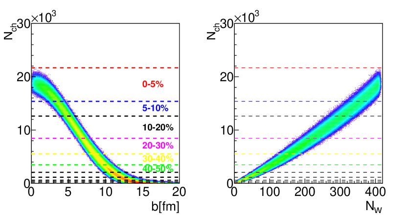
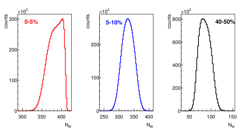
Two-dimensional scatter plots representing the dependence on and of the produced number of charged particles are presented in the left and the right panel of Fig. 1, respectively. The centrality classes, selected by applying sharp cuts on the number of produced charged particles (y axis), are represented by the dashed horizontal lines. As seen from the scatter plots in the Fig. 1, where each dot represents one single event, the impact parameter as well as the number of wounded nucleons fluctuate from event-to-event, thus generating a distribution. To demonstrate this explicitly we present, in Fig. 2, distributions of wounded nucleons for 3 different centrality classes.
For the most central collisions we observe that the distribution is asymmetric and has a tail towards lower values of wounded nucleons. This is caused by the fact that the number of wounded nucleons cannot exceed two times the mass number of the colliding nuclei, i.e. , in the case of collisions. As a consequence, higher cumulants of the distribution of wounded nucleons acquire large values for this centrality bin. This, in turn, distorts the experimentally measured cumulants of both particles and net-particles. Indeed, according to eqs. 22- 24, the cumulants of the participant distributions are entering into the measured cumulants of net-particles . In the following, we will study these contributions based on experimental measurements of the distributions of protons and antiprotons at the LHC and RHIC, respectively.
IV.1 LHC energies
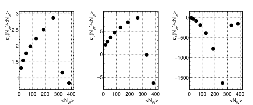
The centrality dependence of cumulants of the wounded nucleon distributions, normalised to the mean number of wounded nucleons, are presented in Fig. 3.
Protons and antiprotons are produced from each wounded nucleon or ’mini-fireball’ within the framework of the Grand Canonical Ensemble. In doing so we first define two independent Poisson distributions; one for protons and another one for antiprotons. The mean values of protons and antiprotons, which define the corresponding Poisson distributions, are taken from the ALICE measurements in collisions at TeV ALICE_Multiplicities . We assume that the first moment of the net-proton distribution vanishes, hence we take the same mean number of antiprotons and protons, which is quantitatively supported by both experimental measurements ALICE_Multiplicities and Hadron Resonance Gas model analysis, see HRG . Next, for each source we generate protons and antiprotons from independent Poisson distributions. Each generated event is thus characterised by the number of wounded nucleons (different for each event), as well as the resulting number of protons and antiprotons. The event averages of these quantities, with simulated events, expressed in terms of cumulants of protons and net-protons are presented in Figs. 4- 6. Here, red symbols represent results computed under the assumption of keeping the number of wounded nucleons fixed, while black symbols correspond to the full simulation, i.e., wounded nucleons fluctuate from event to event. We note that as a fixed number of wounded nucleons we used their values averaged over all events. Black lines are calculated using eqs. 22 - 24, where for protons and were used.

As is seen from the left panel of Fig. 4, the second cumulants of protons are modified by the fluctuations of wounded nucleons. Moreover, starting from the third centrality class, the centrality bin width used in the data analysis is doubled (see Fig. 1), leading to enhanced fluctuations in the distributions of wounded nucleons. This is the reason for the kink-like structure in the centrality dependence of the second cumulants for protons presented in the left panel of the Fig. 4. The contribution from wounded nucleon fluctuations to the second cumulants of protons, encoded in the second cumulants of wounded nucleons , are scaled with the square of the mean number number of protons from each wounded nucleon (cf. eq. 22). On the other hand, as mentioned above, at ALICE energies the mean number of protons and anti-protons are nearly identical, see ALICE_Multiplicities and HRG , implying that the participant fluctuation part for the second cumulants of net-proton distributions vanishes. As a consequence, the second cumulants of net-protons at ALICE energies are not affected by the fluctuations of wounded nucleons, as demonstrated in the right panel of the Fig. 4, where the red and black symbols coincide.
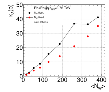
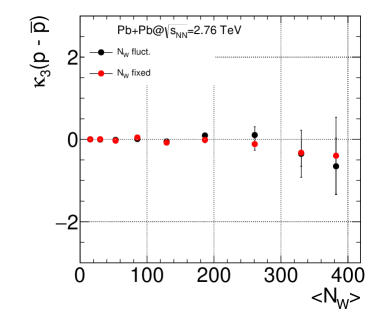
In Fig. 5, the centrality dependence for the third cumulants of protons and net-protons are presented. We again observe strong contributions from the fluctuations of wounded nucleons which are evidenced by differences between the red and black distributions for protons. Furthermore, the variation in the width of the centrality class leads to an even more pronounced kink structure, which in turn makes the centrality dependence non-monotonic. Fortunately, for the third moments of the net-proton distributions at ALICE energies, the contributions from participant fluctuations still vanish.
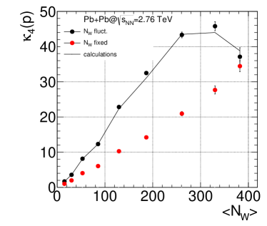
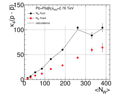
This is because, in eq. 23, the cumulants of the participants are scaled with the mean number of net-protons. The situation changes significantly for the fourth cumulants of net-protons. Our calculations demonstrate that, for the fourth cumulants, the contributions from participant fluctuations are not removed even for vanishing mean value of net-particles. Indeed, by setting in eq. 24 we obtain for the fourth cumulants of net-protons:
| (27) |
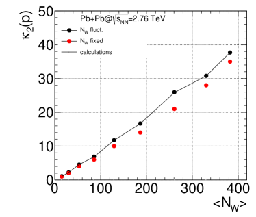
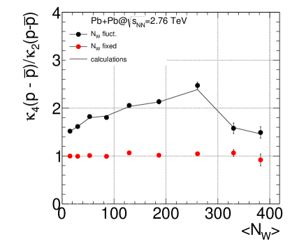
Here, the first term corresponds to the dynamical fluctuations we are interested in. Unless corrected, this gets masked by the second term that includes the second cumulant of participant distributions. The latter is quite significant as seen in the right panel of Fig. 6, where the black line (very close to the symbols) is plotted using eq. 27. In the left panel of Fig. 6 fourth cumulants of protons are presented. For the first centrality bin (0-5) we observe rather small difference between red and black symbols. This is because fourth cumulants of protons gets modified by , and (cf. eq. 24). On the other hand, as seen in Fig. 3, both and are negative for this centrality bin. The interplay between mean number of protons and cumulants of wounded nucleons may by chance cancel the effect of volume fluctuations. In Fig. 7 we present the ratio of the fourth and second cumulants of net-protons. Since our simulations involve no dynamical net-proton fluctuations, for fixed number of wounded nucleons the ratio is unity (red points). However, due to participant fluctuations, the results get modified by a factor of more than two (black points). This can also be explained analytically by taking the ratio of the corresponding cumulants in eqs. 24 and 22 for
| (28) |
We thus obtain that, even at ALICE energies, the ratio of the fourth to the second cumulants of net-protons is significantly modified by fluctuations of participants scaled with the second cumulant of net-protons. This implies that the enhancement of the fourth cumulant of net-protons due to participant fluctuations will introduce a significant bias into this cumulant ratio.
IV.2 RHIC energies
We demonstrated in the previous section our results at LHC energies, where the mean number of net-protons is, to a high degree of accuracy, zero. There the influence of participant fluctuations on the second and third net- proton cumulants vanishes. The fourth (and all higher even ) cumulants, however, receive significant contributions from such fluctuations. At lower energies the mean number of net-protons increases, and no such cancellation is expected then even for the 2nd and 3rd cumulants.
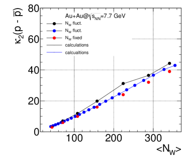
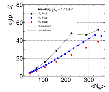
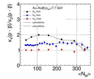
To study this in detail we present, in this section, the results for second, third and fourth cumulants of net-proton distributions for Au-Au collisions at two different values of , namely 39 and 7.7 GeV. The latter value is the lowest energy at which the STAR collaboration has taken data in the framework of the RHIC BES. To this end we have simulated minimum bias Au+Au collisions at = 7.7 and 39 GeV.
In doing so we have neglected any possible correlations between charged particles, employed for the centrality determination, and those used for the event-by-event analysis. Such (auto-)correlations are unavoidable if the rapidity window used for the centrality determination is not sufficiently different from that used for the fluctuation measurements. Mean multiplicities of protons are taken from STARDATA , whereas for anti-protons they are set to zero. As explained in STARDATA , the STAR experimental data points have been modified by the so called Centrality Bin Width Correction (CBWC) CBWC . The essential idea behind the CBWC is to get rid of the participant fluctuations by subdividing a given centrality bin into smaller ones and then merging them together incoherently. In Fig. 8 we present second and third cumulants of net-protons as function of centrality, with variable (black points) and fixed bin width of (blue points).
We observe that the CBWC reduces the overall level of fluctuations significantly but cannot fully eliminate the participant fluctuations. This can also be seen in Fig. 1 from the 2-dimensional scatter plots there, where even for a fixed value of charged particles the number of wounded nucleons still fluctuates. On the other hand, the incoherent addition of data from intervals with very small centrality bin width will likely distort the physics we are after since the correction also eliminates true dynamical fluctuations. The CBWC in particular reduces true dynamical correlations. This is particularly relevant for searches for a critical endpoint in the phase diagram. One of the signatures of such a critical endpoint is that near it the dynamical correlation length will increase rapidly (see above). Since particle production is also likely to be affected, the sensitivity of a search for a critical endpoint will be diminished if too small centrality bins are used.
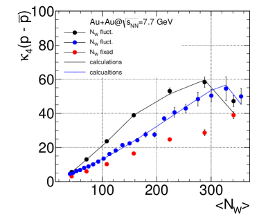
In Fig. 9 we show the results for participant fluctuations for the fourth cumulants of net-protons and their ratio to the second cumulants. Even for very fine centrality bin widths we observe up to deviations from the baseline. Furthermore, participant fluctuations are suppressed less than shown in Figs. 8 and 9 if autocorrelations with the charged particles used for the centrality determination are not removed entirely. We note, in this context, that a significant contribution to net-proton fluctuations will originate from fluctuations of the number of net baryons. This will introduce strong pion-proton correlations into the sample implying that a part of the auto-correlation problem survives, even if one excludes protons and antiprotons from the data used for centrality determination.
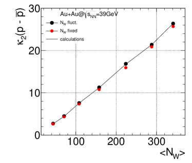
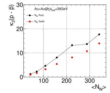
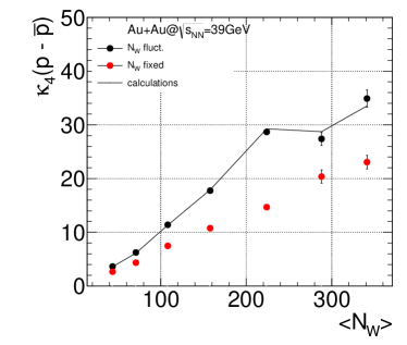
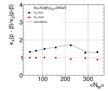
Like in case of protons at TeV (see the left panel of Fig. 6), we observe small effects of the participant fluctuations for the most central bin in Fig. 9. As explained above, this stems from the negative values of and . However, this also depends on the mean number of particles or net-particles. To show this explicitly we present, in Figs. 10 and 11, cumulants of net-protons for Au+Au collisions at =39 GeV. Mean values of protons and antiprotons are taken from STARDATA . For the second cumulants of net-protons we observe quite small contributions from participant fluctuations. However, for the third and fourth cumulants these contributions are significant. Moreover, even for the most central bin deviates from unity if participant fluctuations are included.
V Global conservation laws
In this section we will demonstrate a procedure for selecting an ”optimized” acceptance for fluctuation analysis. For clarity we will focus on net-baryon fluctuations, though our approach is valid for any conserved charges. We remind at this point that critical net-particle fluctuations are predicted within the Grand Canonical Ensemble (GCE) formulation of thermodynamics. In this formulation, the net-baryon number is not conserved in each micro-state, hence it fluctuates. In order to make sense of that, chemical potentials are introduced which guaranties net-baryon number conservation on the average. In order to compare theoretical calculations within GCE, such as HRG model and LQCD, to experimental results, the requirements of GCE have to be achieved in experiments. This is typically done by analysing the experimental data in the finite acceptance by imposing cuts on rapidity and/or mean transverse momentum of detected particles. However, if the selected acceptance window is too small, the possible dynamical correlations we are after will also be strongly reduced KochFluct and consequently, net baryons will be distributed according to the difference of two independent Poisson distributions, the Skellam distribution. This statement is analytically proven below. On the other hand, by enlarging the acceptance, in order to catch dynamical fluctuations, correlations due to baryon number conservation will be significant. The aim of this section is to estimate the contribution from the conservation laws and subtract it from the measured fluctuation signals.
In order to get a quantitative estimate for what means ”large” acceptance we will model the finite acceptance with the binomial distribution.
We first define the acceptance factor for baryons as the ratio of mean number of detected baryons to the number of baryons in the full phase space :
| (29) |
Furthermore, we assume the same acceptance factor for anti-baryons. Given the number of baryons in the full phase space, the probability of measuring baryons in the acceptance is
| (30) |
If the number of baryons in are distributed according to some probability distribution the corresponding multiplicity distribution in the acceptance will then be
| (31) |
The moments of the measured baryon distributions can be then calculated
| (32) |
| (33) |
In a similar way corresponding moments for the anti-baryons can be derived:
| (34) |
| (35) |
Finally, the mixed moment of baryons and anti-baryons are obtained
| (36) |
The second cumulant of net baryons inside the acceptance can be written as
| (37) |
| (38) |
here refers to the second cumulant of the Skellam distribution, which, according to eq. 14 is equal to .
The eq. 38 leads to
| (39) |
because net-baryons do not fluctuate in , i.e, in eq. 38 vanishes.
Eq. 39 shows that fluctuations of net-baryons inside the acceptance will be modified due to the baryon number conservation. Moreover, the modification depends only on the acceptance factor , defined in eq. 29. We first examine a number of useful properties of eqs. 38 and 39. When approaches zero the eq. 39 converges to unity. This means that, in a small acceptance, net-baryon distributions can be described with the Skellam probabilities. On the other hand, with increasing , the fluctuations of net-baryons decrease because of the increasingly significant effect of overall baryon number conservation, and eventually vanish when becomes 1. Moreover, from eq. 38 it is evident that, if in a larger acceptance the net-baryon fluctuations follow the Skellam distribution, then in any smaller acceptance the multiplicities will also be distributed according to the Skellam distribution. Indeed, in this case which leads to . The latter is important and once again underlines the importance of large acceptance.
Experiments typically report on net-proton cumulants which are used as a proxy for the net-baryons. The validity of this assumption is fulfilled at the LHC energies Kitazawa . In order to correct net proton distributions for the baryon number conservation eq. 39 can still be employed by redefining the the (see eq. 29) parameter as
| (40) |
where, refers to the mean number of protons inside the acceptance.
VI Conclusion
In summary, we studied non-dynamical contributions to fluctuations of net-protons within the Wounded Nucleon Model. Since the impact parameter is not measurable in a nuclear collision such fluctuations of participants cannot be avoided experimentally. To study their impact, we developed a Monte Carlo method to describe realistically the centrality dependence of the collision geometry and its influence on higher moments of net-baryon distributions. To this end we provide analytic relations between net-particle and wounded nucleon cumulants for any cumulant order. Furthermore, we discuss a procedure for selecting an ’optimal’ acceptance for fluctuation measurements.
The results of our studies exhibit a strong centrality and energy dependence for these non-dynamical fluctuations. The magnitude of the effect is very significant, exceeding the fluctuations computed for a non-interacting hadron resonance gas by more than a factor of 2. Only for the case of vanishing mean values of net-protons, as observed at mid-rapidity for LHC energies, their second and third cumulants are found to be independent of participant fluctuations, while higher even moments are significantly affected. At lower energies, where the mean numbers of protons and antiprotons are different, the second and all higher cumulants depend strongly on fluctuations of wounded nucleons (or participants). The simplest way to use our approach in the interpretation of experimental data is to start from a particular theoretical prediction and fold the results with our calculations for fluctuations of participants and conservation of net-baryon number before any detailed comparison with experiment. A more ambitious and ultimately necessary program would be to unfold experimental data in the inverse approach. This will require a very detailed understanding of experimental resolutions and efficiencies. The effects we have observed, in particular for higher than 2nd cumulants, are so significant at all beam energies that their inclusion into analysis procedures seem mandatory before quantitative physics conclusions from fluctuation data can be obtained.
VII ACKNOWLEDGMENTS
This work is part of and supported by the DFG Collaborative Research Centre ”SFB 1225 (ISOQUANT)”. The authors acknowledge stimulating discussions with Bengt Friman, Volker Koch, and Krzysztof Redlich. One of us (pbm) would like to thank Jochen Thaeder for insightful remarks concerning the intricacies of fluctuation analyses.
References
- (1) M. Stephanov, K. Rajagopal, and E. Shuryak, Phys. Rev. Lett. 81 (1998) 4816, Phys. Rev. D60 (1999) 114028.
- (2) C. Athanasiou, K. Rajagopal, and M. Stephanov, Phys.Rev. D82 (2010) 074008.
- (3) E. V. Shuryak, M. A. Stephanov, Phys.Rev. C63 (2001) 064903.
- (4) A. Bazavov et al. (HotQCD Collab.), Phys.Rev. D86 (2012) 034509.
- (5) P. Braun-Munzinger, A. Kalweit, K. Redlich, and J. Stachel, Phys.Lett. B747 (2015) 292.
- (6) M. Cheng et al., Phys.Rev. D79 (2009) 074505.
- (7) R. V. Gavai and S. Gupta, Phys. Lett. B696 (2011) 459, arxiv: 0909.4630v1.
- (8) A. Bzdak, V. Koch, and V. Skokov, Phys. Rev. C87 (2013), 014901.
- (9) M. I. Gorenstein, and M. Gazdzicki, Phys. Rev. C84 (2011) 014904.
- (10) V. Begun, arXiv:1606.05358.
- (11) V. Skokov, B. Friman, and K. Redlich, Phys.Rev. C88 (2013) 034911.
- (12) M. Abramowitz, and I. A. Stegun (Eds.), Handbook of Mathematical Functions with Formulas, Graphs, and Mathematical Tables (Dover Publications Inc., New York, 1972), p. 928.
- (13) A. Bialas, and M. Bleszynski, W. Czyz, Nucl. Phys. B111 (1976) 461.
- (14) B. Abelev et al. (ALICE Collab.), Phys. Rev. C88 (2013) 044909.
- (15) D. Kharzeev, E. Levin, and M. Nardi, Nucl. Phys. A747 (2005) 609.
- (16) W. Deng, X. Wang, and R. Xu, Phys. Rev. C83 (2011) 014915, arXiv:1008.1841 [hep-ph].
- (17) B. Alver, M. Baker, C. Loizides, and P. Steinberg, arXiv:0805.4411 [nucl-ex].
- (18) B. Abelev et al. (ALICE Collab.), Phys. Rev. C88 (2013) 044910.
- (19) A. Andronic, P. Braun-Munzinger, K. Redlich, and J. Stachel, proceedings of SQM 2016, arXiv:1611.01347.
- (20) X. Luo, PoS(CPOD2014)019, arXiv:1503.02558.
- (21) X. Luo, J. Xu, B. Mohanty, and N. Xu, J.Phys. G40 (2013) 105104.
- (22) V. Koch, in ”Relativistic Heavy Ion Physics”, R. Stock (ed.) (Springer, Heidelberg, 2010), (Landolt-Boernstein New Series I, v. 23) p. 626, arXiv:0810.2520v1.
- (23) M. Kitazawa, and M. Asakawa, Phys. Rev. C86 (2012) 024904 and erratum, ibidum 069902, arXiv:1205.3292 [nucl-th].