Deeply quasi-bound state in single- and double-$\bar{K}$ nuclear clusters

Abstract

New calculations of the quasi-bound state positions in $K^{-}K^{-}pp$ kaonic nuclear cluster are performed using non-relativistic four-body Faddeev-type equations in AGS form. The corresponding separable approximation for the integral kernels in the three- and four-body kaonic clusters is obtained by using the Hilbert-Schmidt expansion procedure. Different phenomenological models of $\bar{K}N-\pi\Sigma$ potentials with one- and two-pole structure of $\Lambda$(1405) resonance and separable potential models for $\bar{K}$-$\bar{K}$ and nucleon-nucleon interactions, are used. The dependence of the resulting four-body binding energy on models of $\bar{K}N-\pi\Sigma$ interaction is investigated. We obtained the binding energy of the $K^{-}K^{-}pp$ quasi-bound state $\sim$ 80-94 MeV with the phenomenological $\bar{K}N$ potentials. The width is about $\sim$ 5-8 MeV for the two-pole models of the interaction, while the one-pole potentials give $\sim$ 24-31 MeV width.

I Introduction

Over the past two decades, much attention has been placed on the studying of antikaon-nucleon and -nucleus interaction and the formation of dense $\bar{K}$ nuclear clusters akaishi ; yamazaki1 ; dote1 . The $K^{-}pp$ is the lightest possible kaonic nuclear bound system in which the proportion of strongly attractive $\bar{K}N$ ($I=0$) pairs to less attractive $\bar{K}N$ ($I=1$) pairs is maximized. Many theoretical works mostly focusing on the lightest kaonic system have been performed dote1 ; dote2 ; shev1 ; shev2 ; revai ; ikeda1 ; ikeda2 ; ikeda3 ; maeda . All calculations confirm the existence of quasi-bound state in the $K^{-}pp$ system, but the values of the binding energy and width vary over a fairly wide range.

From the experimental point of view, this issue has also attracted considerable attention. The first experimental evidence concerning $K^{-}pp$ was observed in the stopped $K^{-}$ on $\mathrm{{}^{6,7}{Li}}$ and $\mathrm{{}^{12}{C}}$ targets angello by FINUDA collaboration at DA$\mathrm{\Phi}$NE. An exclusive analysis of the $p+p\rightarrow{X}+K^{+},X\rightarrow{p}+\Lambda$ experiment at Saclay for the $pp$ reaction at 2.85 GeV yamazaki2 indicated a large peak both in the $\Lambda{p}$ invariant-mass and $K^{+}$ missing-mass spectra, which had been predicted in the theoretical works yamazaki3 ; yamazaki4 . Only when the object $X$ is a dense bound state of $K^{-}pp$ system, a peak comparable to the free emission of the $\Lambda^{\star}$ would be observed. The $K^{-}pp$ quasi-bound state has been further explored at J-PARC through $d(\pi^{+},K^{+})K^{-}pp$ and $K^{-}+\mathrm{{}^{3}{He}}$ reactions by E27 nagae2 and E15 hiraiwa2 experiments, respectively. However, so far the experimental studies on binding and width of $K^{-}pp$ neither agree with theoretical predictions nor their results are in accordance with each other.

The $\bar{K}\bar{K}N$ system by quantum numbers $J^{\pi}=\frac{1}{2}^{+}$ and $I=\frac{1}{2}$ is also a possible three-body kaonic system. The $\bar{K}\bar{K}N$ quasi-bound state has been studied by Shevchenko and Haidenbauer using phenomenological and chiraly motivated potentials for the $\bar{K}N-\pi\Sigma$ interaction combined with Faddeev AGS equations shev5 . This has also been investigated by Kanada-En’yo and Jido using a Gaussian expansion method kanada . In both studies, a quasi-bound state was found in the $\bar{K}\bar{K}N$ three-body system just a few MeV below the $\Lambda(1405)+\bar{K}$ threshold energy and it was shown that the repulsive interaction in $\bar{K}\bar{K}$ with $I=1$ makes the $\bar{K}\bar{K}N$ system loosely bound with moderate binding energy. The natural question which arises now is what will happen if we add an antikaon to the $K^{-}pp$ or a proton to the $K^{-}K^{-}p$ three-body system. In 2004, Akaishi and Yamazaki investigated the simplest double-$\bar{K}$ nuclear cluster, $K^{-}K^{-}pp$, using a phenomenological interaction based on the G-matrix method yamaz . They have shown that this system is deeply bound with binding energy of 117 MeV and could be considered as an important doorway toward multi-$\Lambda^{\star}$ nuclei. The existence of such a deeply kaonic nuclear state is important for studying high-density $\bar{K}$-nuclear systems yamaz , kaon condensation issue and neutron strars kaplan .

In this paper, we performed the nonrelativistic Faddeev-type Alt-Grassberger-Sandhas (AGS) calculations for the $K^{-}pp$ and $K^{-}K^{-}p$ three-body systems as well as for $K^{-}K^{-}pp$ four-body system. To convert the few-body Faddeev AGS equations to a manageable set of equations, we have to introduce the separable representation of the few-body amplitudes and the driving terms, which will be necessary to find the pole position of kaonic nuclear systems grass ; nadro . Our few-body Faddeev calculations is based on the quasi-particle method. Using this method, we can find a separable representation for the subamplitudes in (3+1) and (2+2) partitions and one can reduce the three- and four-body problem to an effective quasi-particle two-body one, where one of the components appears as a quasi-particle. For making a separable representation of these subsystem amplitudes, one can use the energy dependent pole expansion (EDPE) sofia or the Hilbert-Schmidt expansion nadro . For this purpose, we will apply the Hilbert-Schmidt expansion.

The dependence of the three- and four-body kaonic clusters pole positions on two-body interactions is investigated. Several models of $\bar{K}N-\pi\Sigma$ interactions, which are derived phenomenologicaly, are used shev3 ; shev4 . The potentials reproduce experimental data on elastic and inelastic $K^{-}p$ cross-sections and kaonic hydrogen atom. The $\bar{K}N-\pi\Sigma$ potentials are also constructed to produce a one- or two-pole structure of $\Lambda(1405)$ resonance. The double-$\bar{K}$ clusters contain the repulsive $\bar{K}\bar{K}$ interaction. Thus, the question which arises now is how much this interaction is important in double kaonic systems under study. In our few-body calculations, we used a phenomenological potential for the repulsive $\bar{K}\bar{K}$ interaction and the parameters of the potential obtained in such a way to reproduce the scattering length of the lattice QCD calculations bean .

The paper is organized as follows: in sect. II, we describe the framework of the present calculation and a brief description of Faddeev equations in the AGS form for three- and four-body kaonic nuclear systems is presented. Sect. III is devoted to introducing the two-body inputs of the calculations. In sect. IV, we present our results of the three- and four-body calculations and the conclusions are presented in sect. V.

II Formalism

II.1 Three-body equations

The $\bar{K}NN$ and $\bar{K}\bar{K}N$ systems are coupled to $\pi\Sigma{N}$ and $\pi\bar{K}\Sigma$ channels, respectively. The three-body Faddeev-type AGS equations grass ; alt for these systems are

$$U_{ij}^{\alpha\beta}=(1-\delta_{ij})\delta_{\alpha\beta}G_{0}^{-1}\sum_{k=1}^{3}\sum_{\gamma=1}^{3}(1-\delta_{ik})T_{k}^{\alpha\gamma}G_{0}^{\gamma}U^{\gamma\beta}_{kj},$$ (1)

where the operators $U^{\alpha\beta}_{ij}$ give the Faddeev amplitudes of the elastic and re-arrangement processes $i^{\alpha}+(j^{\alpha}k^{\alpha})\rightarrow{j}^{\beta}+(k^{\beta}i^{\beta})$ and the operators $T_{k}^{\alpha\gamma}$ are the two-body $T$-matrices embedded in the three-body space. The operator $G^{\alpha}_{0}$ is the free three-body Green’s function; and the indices $i,j=1,2,3$ and $\alpha,\beta=1,2,3$ are used for describing the Faddeev partitions and particle channels, respectively shev2 . Using the separable potentials for the two-body interactions

$$V_{i,I_{i}}^{\alpha\beta}(k,k^{\prime})=g_{i,I_{i}}^{\alpha}(k_{\alpha})\lambda_{i,I_{i}}^{\alpha\beta}g_{i,I_{i}}^{\beta}(k^{\prime}_{\beta}),$$ (2)

will lead to a separable form of two-body $T$-matrices:

$$T_{i,I_{i}}^{\alpha\beta}(k,k^{\prime};z)=g_{i,I_{i}}^{\alpha}(k_{\alpha})\tau_{i,I_{i}}^{\alpha\beta}(z)g_{i,I_{i}}^{\beta}(k^{\prime}_{\beta}),$$ (3)

where $I$ is a two-body isospin, $g^{\alpha}(k_{\alpha})$ are the usual form factors and $\tau_{i,I_{i}}^{\alpha\beta}$ being the usual two-body propagator. The three-body coupled channels Faddeev AGS equations for $\bar{K}NN-\pi\Sigma{N}$ and $\bar{K}\bar{K}N-\pi\bar{K}\Sigma$ systems are

$$\mathcal{K}_{ij,I_{i}I_{j}}^{\alpha\beta}=\delta_{\alpha\beta}\mathcal{M}_{ij,I_{i}I_{j}}^{\alpha\beta}+\sum_{k,I_{k};\gamma}\mathcal{M}_{ik,I_{i}I_{k}}^{\alpha}\tau_{k,I_{k}}^{\alpha\gamma}\mathcal{K}_{kj,I_{k}I_{j}}^{\gamma\beta},$$ (4)

where the operator $\mathcal{K}_{ij,I_{i}I_{j}}^{\alpha\beta}$ is Faddeev transition amplitude between $\alpha$ and $\beta$ channels and the operator $\mathcal{M}_{ij,I_{i}I_{j}}^{\alpha\beta}$ is the effective potential, which are defined by

$$\mathcal{K}_{ij;I_{i}I_{j}}^{\alpha\beta}=\langle{g}^{\alpha}_{i,I_{i}}|G_{0}^{\alpha}U_{ij;I_{i}I_{j}}G_{0}^{\beta}|{g}^{\alpha}_{j,I_{j}}\rangle,$$ (5)

$$\mathcal{M}_{ij,I_{i}I_{j}}^{\alpha\beta}=\delta_{\alpha\beta}\mathcal{M}_{ij,I_{i}I_{j}}^{\alpha}=\delta_{\alpha\beta}(1-\delta_{ij})\langle{g}^{\alpha}_{i,I_{i}}|G_{0}^{\alpha}|{g}^{\alpha}_{j,I_{j}}\rangle.$$ (6)

The most important part of the quasi-particle approach is the separable representation of the off-shell Faddeev amplitudes in the two- and three-body systems. First of all, we will introduce the separable form of the three-body amplitudes and driving terms, for the $\bar{K}NN$ and $\bar{K}\bar{K}N$ systems by applying Hilbert-Schmidt expansion (HSE) nadro .

$$\mathcal{M}_{ij,I_{i}I_{j}}^{\alpha}(p,p^{\prime},\epsilon)=-\sum^{N_{r}}_{n=1}\lambda_{n}(\epsilon)u_{n;i,I_{i}}^{\alpha}(p,\epsilon)u_{n;j,I_{j}}^{\alpha}(p^{\prime},\epsilon),$$ (7)

where $\lambda_{n}$ and the form factors $u_{n;i,I_{i}}^{\alpha}(p,\epsilon)$ are the eigenvalues and eigenfunctions of the kernel of equation (4), respectively. The separable representation of the Faddeev AGS amplitudes is given by

$$\mathcal{K}_{ij,I_{i}I_{j}}^{\alpha\beta}(p,p^{\prime},\epsilon)=\sum^{N_{r}}_{n=1}u_{n;i,I_{i}}^{\alpha}(p,\epsilon)\zeta_{n}(\epsilon)u_{n;j,I_{j}}^{\beta}(p^{\prime},\epsilon),$$ (8)

and the functions $\zeta_{n}(\epsilon)$ obey the equation

$$\zeta_{n}(\epsilon)=\lambda_{n}(\epsilon)/(\lambda_{n}(\epsilon)-1).$$ (9)

To search for a quasi-bound state, we should look for a solution of the homogeneous equations related to the form factors $u_{n;i,I_{i}}^{\alpha}(p,\epsilon)$

$$u_{n;i,I_{i}}^{\alpha}=\frac{1}{\lambda_{n}}\sum_{k=1}^{3}\sum_{\gamma=1}^{3}\sum_{I_{k}}\mathcal{M}_{ik,I_{i}I_{k}}^{\alpha}\tau_{k,I_{k}}^{\alpha\gamma}u_{n;k,I_{k}}^{\gamma}.$$ (10)

The AGS equation of (10) is a Fredholm type integral equation. To solve the AGS equations for both $\bar{K}NN$ and $\bar{K}\bar{K}N$ systems, the operators involving two identical nucleons and kaons should be antisymmetric and symmetric, respectively. In $\bar{K}\bar{K}N$ system, the kaons are spinless particles, then all operators in isospin base involving two kaons, should be symmetric while in the case of $\bar{K}NN$, the spin component is antisymmetric (spin $s=0$). Thus, all operators in isospin base should be symmetric. To find a quasi-bound state in $\bar{K}NN$ and $\bar{K}\bar{K}N$ systems, one should convert the integral equations into algebraic form and then search for a complex energy at which the determinant of the kernel matrix is equal to zero.

II.2 Four-body equations

In the present subsection, we briefly outline the formal aspects of the four-body Faddeev formalism applying to $\bar{K}\bar{K}NN$ system within the quasi-particle method in momentum space. Although a variety of methods for studying the four-body systems has been proposed in the literature, the Faddeev AGS method grass ; alt and Faddeev-Yakubovsky approach yak1 ; yak2 are more preferable to other methods. Using the separable approximation for the two-body potentials and for Faddeev amplitudes appearing in different K-type and H-type partitions of the four-body system, the both Faddeev approaches will produce the same set of effective two-body equations grass ; nadro ; fonse . Although the structure of the four-body equations are much more complicated compared to the three-body case, but currently, a practical formalism of four-particle theory has been extensively developed. Using properly symmetrized and antisymmetrized states with respect to identical kaons and nucleons, we will have the following four channels, corresponding to four possible two-quasiparticle partitions of $\bar{K}\bar{K}NN$ system. In fig. 1, one K-type ($\bar{K}+[\bar{K}NN]$) and one H-type ($[\bar{K}N]+[\bar{K}N]$) configurations of the $\bar{K}\bar{K}NN$ four-body system are shown. The whole dynamics of $\bar{K}\bar{K}NN$ system is described in terms of the transition amplitudes $\mathcal{A}_{\alpha 1}$ ($\alpha=$1,2,3 and 4) which connect the four quasi-two-body channels characterized by

$$\begin{split}&\alpha=1:\bar{K}+(\bar{K}NN),\ \ \alpha=2:N+(\bar{K}\bar{K}N),\\ &\alpha=3:(\bar{K}N)+(\bar{K}N),\ \ \alpha=4:(\bar{K}\bar{K})+(NN),\end{split}$$ (11)

with the initial channel $\alpha=1$. The essence of the calculation scheme is the solution of the bound state problem for the two- and three-body subsystems that is specified in the partitions (11). For $\alpha=1$ and 2 we dealt with interacting three-body systems. Using separable representations for the $NN$ and $\bar{K}N$ potentials, the corresponding scattering amplitudes can be expressed in terms of effective quasi-two-body amplitudes $\mathcal{K}^{\alpha\beta}_{ij,I_{i}I_{j}}$ which describe the scattering of a particle on a two-body cluster (quasi-particle). Due to the strong dominance of s-waves in $\bar{K}N$ and $NN$ interactions, we take into account only the s-wave part of the interactions in two, three and four-particle states. Then, we drop the index $l=0$ in all equations. Considering the identity of the kaons and the nucleons, the $\bar{K}\bar{K}NN$ problem is reduced to a set of $4\times 4$ integral equations in one scalar variable. For the transition amplitudes $\mathcal{A}_{\alpha 1}$ as a connector of channel 1 to channels $\alpha=$1, 2, 3 and 4, we arrive at a coupled set of equations

$$\begin{split}&\mathcal{A}^{sI,s^{\prime}I^{\prime}}_{\alpha\beta,nn^{\prime}}(p,p^{\prime},E)=\mathcal{R}^{sI,s^{\prime}I^{\prime}}_{\alpha\beta,nn^{\prime}}(p,p^{\prime},E)\\ &\hskip 71.13188pt+\sum^{3}_{\gamma=1}\sum_{n^{\prime\prime}s^{\prime\prime}I^{\prime\prime}}\int^{\infty}_{0}\mathcal{R}^{sI,s^{\prime\prime}I^{\prime\prime}}_{\alpha\gamma,nn^{\prime\prime}}(p,p^{\prime\prime},E)\\ &\hskip 71.13188pt\times\zeta_{\gamma,n^{\prime\prime}}(\epsilon_{\gamma})\mathcal{A}^{s^{\prime\prime}I^{\prime\prime},s^{\prime}I^{\prime}}_{\gamma\beta,n^{\prime\prime}n^{\prime}}(p^{\prime\prime},p^{\prime},E)d\vec{p^{\prime\prime}},\end{split}$$ (12)

where the operators $\mathcal{A}^{sI,s^{\prime}I^{\prime}}_{\alpha\beta,nn^{\prime}}$ are the Faddeev amplitudes. The operators $\mathcal{R}^{sI,s^{\prime}I^{\prime}}_{\alpha\beta,nn^{\prime}}$ are the effective potentials that are realized through particle exchange between the quasi-particles in channels $\alpha$ and $\beta$ and the arguments $\zeta_{\alpha,n}$ are the effective propagators, which are given in (9). The AGS equations (12) for the $\bar{K}\bar{K}NN$ system are schematically illustrated in fig. 2.

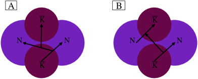
Figure 1: Two different rearrangement channels of $\bar{K}\bar{K}NN$ four-body system. (A) Channel 1, a two-body channel of (1+3) type (K-type); (B) channel 3, a two-body channel of (2+2) type (H-type). Antisymmetrization and symmetrization is to be made between two nucleons and between two kaons, respectively.

The effective potentials $\mathcal{R}^{sI,s^{\prime}I^{\prime}}_{\alpha\beta,nn^{\prime}}(p,p^{\prime},E)$ can be expressed in terms of the form factors $u^{sI}_{\alpha,n}$, which are generated by the separable representation of the sub-amplitudes appearing in the channels (11)

$$\begin{split}&\mathcal{R}^{sI,s^{\prime}I^{\prime}}_{\alpha\beta,nn^{\prime}}(p,p^{\prime},E)=\frac{\Omega_{sI,s^{\prime}I^{\prime}}}{2}\int^{+1}_{-1}u^{sI}_{\alpha,n}(\vec{q},\epsilon_{\alpha}-\frac{p^{2}}{2\mathcal{M}_{\alpha}})\\ &\times\tau(z=E-\omega(p,p^{\prime}))u^{s^{\prime}I^{\prime}}_{\beta,n^{\prime}}(\vec{q^{\prime}},\epsilon_{\beta}-\frac{p^{\prime 2}}{2\mathcal{M}_{\beta}})d(\hat{\vec{p}}\cdotp\hat{\vec{p}}^{\prime}).\end{split}$$ (13)

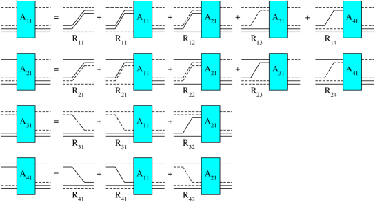
Figure 2: Diagrammatic representation of the equations (12) for the Faddeev amplitudes $\mathcal{A}_{\alpha 1}$ of the $\bar{K}\bar{K}NN$ system.

Here, the symbols $\Omega_{sI,s^{\prime}I^{\prime}}$ are the spin-isospin Clebsch-Gordan coefficients, the argument $z=E-\frac{p^{2}}{2M_{\beta}}-\frac{p^{\prime 2}}{2M_{\alpha}}-\frac{\vec{p}\cdot\vec{p}^{\prime}}{m}$ is the energy of two-body quasi-particle, embedded in the four-body space and $\epsilon_{\alpha}$ is the total energy of the subsystem in channel $\alpha$. The effective potentials for $\bar{K}\bar{K}NN$ system are represented by the particle exchange diagrams in fig. 3. The momenta $\vec{q}(\vec{p},\vec{p}^{\prime})$ and $\vec{q}^{\prime}(\vec{p},\vec{p}^{\prime})$ are given in terms of $\vec{p}$ and $\vec{p^{\prime}}$ by the following relations

$$\vec{q}=\vec{p}^{\prime}+\frac{M_{\alpha}}{m}\vec{p},\ \ \ \ \ \ \vec{q}^{\prime}=\vec{p}+\frac{M_{\beta}}{m}\vec{p}^{\prime},$$ (14)

where $m$ is the exchanged particle or quasi-particle mass and the reduced masses $\mathcal{M}_{\alpha}$ and $M_{\alpha}$ in channel $\alpha$ are defined by

$$\begin{split}&\mathcal{M}_{\alpha}=m^{\alpha}_{i}(m^{\alpha}_{j}+m^{\alpha}_{k}+m^{\alpha}_{l})/(m^{\alpha}_{i}+m^{\alpha}_{j}+m^{\alpha}_{k}+m^{\alpha}_{l}),\\ &M_{\alpha}=m^{\alpha}_{j}(m^{\alpha}_{k}+m^{\alpha}_{l})/(m^{\alpha}_{j}+m^{\alpha}_{k}+m^{\alpha}_{l}),\end{split}$$ (15)

and in the case of H-type subsystems are given by

$$\begin{split}&\mathcal{M}_{\alpha}=(m^{\alpha}_{i}+m^{\alpha}_{j})(m^{\alpha}_{k}+m^{\alpha}_{l})/(m^{\alpha}_{i}+m^{\alpha}_{j}+m^{\alpha}_{k}+m^{\alpha}_{l}),\\ &M_{\alpha}=m^{\alpha}_{i}m^{\alpha}_{j}/(m^{\alpha}_{i}+m^{\alpha}_{j}).\end{split}$$ (16)

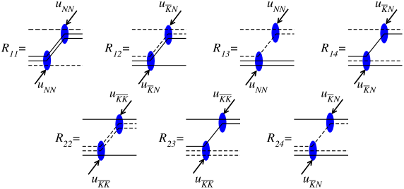
Figure 3: Diagrammatic representation of the potentials $\mathcal{R}_{\alpha\beta}$ in the separable approximation. The dashed line corresponds to the $\bar{K}$ and the solid lines corresponds to the nucleon. The symbols $u_{\alpha}$ define the initial and final states of the system.

Table 1: Table of symbols that appear in the effective potentials $\mathcal{R}_{\alpha\beta}$. The symbols related to the driving terms $\mathcal{R}_{\beta\alpha}$, can be defined in a similar way.

$\mathcal{R}^{sI,s^{\prime}I^{\prime}}_{\alpha\beta,nn^{\prime}}$	$\vec{q}$	$\vec{q}^{\prime}$	$\omega(p,p^{\prime})$
$\mathcal{R}^{sI,s^{\prime}I^{\prime}}_{11,nn^{\prime}}$	$\vec{p}^{\prime}+\frac{M_{\bar{K}}}{M_{\bar{K}}+2M_{N}}\vec{p}$	$\vec{p}+\frac{M_{\bar{K}}}{M_{\bar{K}}+2M_{N}}\vec{p}^{\prime}$	$\frac{p^{2}(M_{\bar{K}}+2M_{N})}{2M_{\bar{K}}(M_{N}+M_{N})}+\frac{p^{\prime 2}(M_{\bar{K}}+2M_{N})}{2M_{\bar{K}}(2M_{N})}+\frac{\vec{p}\cdot\vec{p}^{\prime}}{M_{N}+M_{N}}$
$\mathcal{R}^{sI,s^{\prime}I^{\prime}}_{12,nn^{\prime}}$	$\vec{p}^{\prime}+\frac{M_{N}}{M_{\bar{K}}+2M_{N}}\vec{p}$	$\vec{p}+\frac{M_{\bar{K}}}{M_{N}+2M_{\bar{K}}}\vec{p}^{\prime}$	$\frac{p^{2}(M_{N}+2M_{\bar{K}})}{2M_{\bar{K}}(M_{N}+M_{\bar{K}})}+\frac{p^{\prime 2}(M_{\bar{K}}+2M_{N})}{2M_{N}(M_{N}+M_{\bar{K}})}+\frac{\vec{p}\cdot\vec{p}^{\prime}}{M_{N}+M_{\bar{K}}}$
$\mathcal{R}^{sI,s^{\prime}I^{\prime}}_{13,nn^{\prime}}$	$\vec{p}^{\prime}+\frac{2M_{N}}{M_{\bar{K}}+2M_{N}}\vec{p}$	$\vec{p}+\frac{1}{2}\vec{p}^{\prime}$	$\frac{p^{2}}{M_{\bar{K}}}+\frac{p^{\prime 2}(M_{\bar{K}}+2M_{N})}{2M_{\bar{K}}(M_{N}+M_{N})}+\frac{\vec{p}\cdot\vec{p}^{\prime}}{M_{\bar{K}}}$
$\mathcal{R}^{sI,s^{\prime}I^{\prime}}_{14,nn^{\prime}}$	$\vec{p}^{\prime}+\frac{M_{N}+M_{\bar{K}}}{M_{\bar{K}}+2M_{N}}\vec{p}$	$\vec{p}+\frac{M_{\bar{K}}}{M_{\bar{K}}+M_{N}}\vec{p}^{\prime}$	$\frac{p^{2}(M_{N}+M_{\bar{K}})}{2M_{\bar{K}}M_{N}}+\frac{p^{\prime 2}(M_{\bar{K}}+2M_{N})}{2M_{N}(M_{N}+M_{\bar{K}})}+\frac{\vec{p}\cdot\vec{p}^{\prime}}{M_{N}}$
$\mathcal{R}^{sI,s^{\prime}I^{\prime}}_{22,nn^{\prime}}$	$\vec{p}^{\prime}+\frac{M_{N}}{2M_{\bar{K}}+M_{N}}\vec{p}$	$\vec{p}+\frac{M_{N}}{2M_{\bar{K}}+M_{N}}\vec{p}^{\prime}$	$\frac{p^{2}(M_{N}+2M_{\bar{K}})}{2M_{N}(M_{\bar{K}}+M_{\bar{K}})}+\frac{p^{\prime 2}(M_{N}+2M_{\bar{K}})}{2M_{N}(M_{\bar{K}}+M_{\bar{K}})}+\frac{\vec{p}\cdot\vec{p}^{\prime}}{2M_{\bar{K}}}$
$\mathcal{R}^{sI,s^{\prime}I^{\prime}}_{23,nn^{\prime}}$	$\vec{p}^{\prime}+\frac{2M_{\bar{K}}}{2M_{\bar{K}}+M_{N}}\vec{p}$	$\vec{p}+\frac{1}{2}\vec{p}^{\prime}$	$\frac{p^{2}}{M_{N}}+\frac{p^{\prime 2}(M_{N}+2M_{\bar{K}})}{2M_{N}(M_{\bar{K}}+M_{\bar{K}})}+\frac{\vec{p}\cdot\vec{p}^{\prime}}{M_{N}}$
$\mathcal{R}^{sI,s^{\prime}I^{\prime}}_{24,nn^{\prime}}$	$\vec{p}^{\prime}+\frac{M_{N}+M_{\bar{K}}}{M_{N}+2M_{\bar{K}}}\vec{p}$	$\vec{p}+\frac{M_{N}}{M_{\bar{K}}+M_{N}}\vec{p}^{\prime}$	$\frac{p^{2}(M_{N}+M_{\bar{K}})}{2M_{\bar{K}}M_{N}}+\frac{p^{\prime 2}(M_{N}+2M_{\bar{K}})}{2M_{\bar{K}}(M_{N}+M_{\bar{K}})}+\frac{\vec{p}\cdot\vec{p}^{\prime}}{M_{\bar{K}}}$

The corresponding assignments of the various symbols appearing in (13) for each effective potential are represented in table 1. Before we proceed to solve the four-body equations, we also need to know the equations describing two independent pairs of interacting particles $(\bar{K}N)+(\bar{K}N)$ and $(\bar{K}\bar{K})+(NN)$ as input. In $(\bar{K}N)+(\bar{K}N)$ case, the corresponding equations read

$$\mathcal{Y}^{sI,s^{\prime}I^{\prime}}_{\bar{K}N,\bar{K}N}=\mathcal{W}^{sI,s^{\prime}I^{\prime}}_{\bar{K}N,\bar{K}N}+\mathcal{W}^{sI,s^{\prime}I^{\prime}}_{\bar{K}N,\bar{K}N}\tau^{s^{\prime}I^{\prime}}_{NN}\mathcal{Y}^{s^{\prime}I^{\prime},s^{\prime}I^{\prime}}_{\bar{K}N,\bar{K}N},$$ (17)

and the Faddeev equations for $(\bar{K}\bar{K})+(NN)$ system are defined by

$$\begin{split}&\mathcal{Y}^{sI,s^{\prime}I^{\prime}}_{\bar{K}\bar{K},NN}=\mathcal{W}^{sI,s^{\prime}I^{\prime}}_{\bar{K}\bar{K},NN}+\mathcal{W}^{sI,s^{\prime}I^{\prime}}_{\bar{K}\bar{K},NN}\tau^{s^{\prime}I^{\prime}}_{NN}\mathcal{Y}^{s^{\prime}I^{\prime},s^{\prime}I^{\prime}}_{NN,NN},\\ &\mathcal{Y}^{s^{\prime}I^{\prime},s^{\prime}I^{\prime}}_{NN,NN}=\mathcal{W}^{s^{\prime}I^{\prime},sI}_{NN,\bar{K}\bar{K}}\tau^{sI}_{\bar{K}\bar{K}}\mathcal{Y}^{sI,s^{\prime}I^{\prime}}_{\bar{K}\bar{K},NN}.\end{split}$$ (18)

Here, $\mathcal{Y}^{sI,s^{\prime}I^{\prime}}_{i,j}$ are Faddeev amplitudes which describe two independent pairs of interacting particles and $\mathcal{W}^{sI,s^{\prime}I^{\prime}}_{i,j}$ are the effective potentials. Analogous to the treatment in the previous subsection, the separable form of the amplitudes can easily be found

$$\mathcal{Y}_{i,j}^{sI,s^{\prime}I^{\prime}}(p,p^{\prime},\epsilon)=\sum^{N_{r}}_{n=1}u_{n;i}^{sI}(p,\epsilon)\zeta_{n}(\epsilon)u_{n;j}^{s^{\prime}I^{\prime}}(p^{\prime},\epsilon),$$ (19)

where the functions $u_{n;i}^{sI}$ are the eigenfunctions of the kernel of eq. (17)

$$u_{n;i}^{sI}=\frac{1}{\lambda_{n}}\sum_{j=\bar{K}N,NN}\mathcal{W}^{sI,s^{\prime}I^{\prime}}_{i,j}\tau^{s^{\prime}I^{\prime}}_{j}u_{n;j}^{s^{\prime}I^{\prime}}.$$ (20)

Due to the strong coupling between $\bar{K}N$ and $\pi\Sigma$ channels, $\bar{K}\bar{K}NN$ four-body equations would be generalized to include the coupled channels $\bar{K}\bar{K}NN-\pi\bar{K}\Sigma{N}-\pi\pi\Sigma\Sigma$. There are seven different interactions in the lower-lying four-body channels, namely $\pi\pi$, $\pi\bar{K}$, $\pi\Sigma$, $\pi{N}$, $\Sigma\bar{K}$, $\Sigma\Sigma$, $\Sigma{N}$ and $\bar{K}N$. The $\pi\Sigma$ and $\bar{K}N$ interactions are included by using the coupled-channel model for $\bar{K}N-\pi\Sigma$ interaction. In practice, when we include the remaining interactions, the number of channels will increase rapidly and the treatment of the four-body equations turns out to be very complicated. Thus, the remaining interactions in the lower four-body channels are neglected for the system under consideration. This is necessary for faster convergence rate of the results.

Before we proceed to solve the AGS equations (12), we should antisymmetriz and symmetriz the basic amplitudes with respect to the exchange of nucleons and kaons, respectively. In practice to solve the four-body equations, it is necessary to convert the equations to a numerically manageable form by expanding (2+2) and (3+1) sub-amplitudes in eqs. (4), (17) and (18) into separable series of finite rank $N_{r}$. We can use two different types of expansion. One is based on Hilbert-Schmidt expansion nadro method, and another one uses the energy dependent pole expansion (EDPE) sofia . In the present study, we have used Hilbert-Schmidt expansion (HSE) method.

III Two-body input

In this section we shall begin with a survey on the two-body interactions, which are the inputs to our present study. The main $\bar{K}N-\pi\Sigma$ potential is constructed with orbital angular momentum $l=0$ since the interaction is dominated by $s$-wave $\Lambda$(1405) resonance. The $NN$, $\bar{K}\bar{K}$ and $\Sigma{N}-\Lambda{N}$ interactions were also taken in $l=0$ state and the remaining interactions are neglected in our calculations. All separable potentials in momentum representation have the form (2).

III.1 $\bar{K}N-\pi\Sigma$ coupled-channel system

The $\bar{K}N-\pi\Sigma$ interaction is the most important interaction of the three- and four-body kaonic nuclear systems. The $\bar{K}N$ interaction, is usually described either by pure phenomenological or by chirally motivated potentials. In our Faddeev calculations, we used four different effective potentials for the coupled-channel $\bar{K}N-\pi\Sigma$ interaction, having a one- and two-pole structure of the $\Lambda$(1405) resonance. The potentials that we used here for the $\bar{K}N$ interaction are given in refs. shev3 ; shev4 . The parameters of the coupled-channel $\bar{K}N-\pi\Sigma$ potential were fitted to reproduce all existing experimental data on the low-energy $K^{-}p$ scattering and kaonic hydrogen. The fitting was performed by using physical masses in $\bar{K}N$ and $\pi\Sigma$ channels with the inclusion of Coulomb interaction. The parameters of $\bar{K}N-\pi\Sigma$ potential in ref. shev3 , are adjusted to reproduce the most recent experimental results of the SIDDHARTA experiment bazzi and the one in ref. shev4 reproduce the experimental results of the KEK experiment kek1 ; kek2 . The form factors of the one-pole version and the $\bar{K}N$ channel of the two-pole version have a Yamaguchi form

$$g_{I}^{\alpha}(k^{\alpha})=\frac{1}{(k^{\alpha})^{2}+(\Lambda_{I}^{\alpha})^{2}},$$ (21)

while a slightly more complicated form is used for the $\pi\Sigma$ channel

$$g_{I}^{\alpha}(k^{\alpha})=\frac{1}{(k^{\alpha})^{2}+(\Lambda_{I}^{\alpha})^{2}}+\frac{s(\Lambda_{I}^{\alpha})^{2}}{((k^{\alpha})^{2}+(\Lambda_{I}^{\alpha})^{2})^{2}}.$$ (22)

III.2 $NN$ and $\Sigma{N}-\Lambda{N}$ interactions

We also used one-term PEST potential from ref. pest , which is a separable approximation of the Paris model of $NN$ interaction. The strength parameter of PEST $\lambda_{NN}^{I}=-1$, and the form-factor is defined by

$$g_{NN}^{I}(k)=\frac{1}{2\sqrt{\pi}}\sum_{i=1}^{6}\frac{c_{i;I}^{NN}}{(\beta_{i;I}^{NN})^{2}+k^{2}},$$ (23)

where a family of such $c_{i;I}^{NN}$ and $\beta_{i;I}^{NN}$ parameters are given in ref. pest . The on- and off-shell properties of the one-term PEST $NN$ potential is equivalent to the Paris potential up to $E_{lab}\sim 50$ MeV. It reproduces the triplet and singlet $NN$ scattering lengths, $a(^{3}S_{1})=-5.422$ fm and $a(^{1}S_{0})=17.534$ fm, respectively, as well as the deuteron binding energy $B.E_{\mathrm{deu}}=−2.2249$ MeV.

For the $s$-wave $\Sigma{N}-\Lambda{N}$ interaction, we follow the form given in ref. tores ,

$$V_{\alpha\beta}^{I}(k,k^{\prime})=-\frac{C_{\alpha\beta}^{I}}{2\pi^{2}}(\Lambda_{\alpha}\Lambda_{\beta})^{3/2}(\mu_{\alpha}\mu_{\beta})^{-1/2}g_{\alpha}^{I}(k)g_{\beta}^{I}(k^{\prime}),$$ (24)

where the symbols $C_{\alpha\beta}^{I}$ are the coupling constants summarized in table 2, $\mu_{\alpha}$ is the reduced mass for the $\Sigma{N}$ and $\Lambda{N}$ system, the form factor $g_{\alpha}^{I}(k)$ is defined by $g_{\alpha}^{I}(k)=1/(k^{2}+\Lambda_{\alpha}^{2})$, and the range parameters $\Lambda_{\alpha}$ are given by $\Lambda_{\Sigma{N}}=1.27\mathrm{fm}^{-1}$ and $\Lambda_{\Lambda{N}}=1.33\mathrm{fm}^{-1}$.

Table 2: Coupling constants of the $\Sigma{N}-\Lambda{N}$ interactions tores .

$C_{\Sigma{N}-\Sigma{N}}^{I=1/2}$	$C_{\Sigma{N}-\Lambda{N}}^{I=1/2}$	$C_{\Lambda{N}-\Lambda{N}}^{I=1/2}$	$C_{\Sigma{N}-\Sigma{N}}^{I=3/2}$
0.83	0.56	0.49	-0.29

III.3 $\bar{K}\bar{K}$ interaction

In contrast to the $\bar{K}N$ interaction, the amount of data on $\bar{K}$-$\bar{K}$ scattering ($S=-2$) is scarce and the experimental situation is poorer than the above three two-body interactions. We introduce the effective interaction of the subsystem $\bar{K}\bar{K}$ with $I=1$, $V^{I=1}_{\bar{K}\bar{K}}$, in a Yamaguchi form

$$\begin{split}&V^{I=1}_{\bar{K}\bar{K}}(k,k^{\prime})=\lambda^{I=1}_{\bar{K}\bar{K}}g_{\bar{K}\bar{K}}(k)g_{\bar{K}\bar{K}}(k^{\prime}),\\ &\ \ \ \ \ \ \ g_{\bar{K}\bar{K}}(k)=\frac{1}{k^{2}+\Lambda^{2}_{\bar{K}\bar{K}}}.\end{split}$$ (25)

During these calculations, we consider the $\bar{K}\bar{K}$ potentials with the parameters $\lambda^{I=1}_{\bar{K}\bar{K}}$ and $\Lambda_{\bar{K}\bar{K}}$, which reproduce the $K^{+}K^{+}$ scattering length, for which we used the result of lattice QCD calculation as $a_{K^{+}K^{+}}=−0.141$ fm bean as a guideline. The range parameter value 3.5 $\mathrm{fm}^{-1}$ is adopted for $\bar{K}\bar{K}$ interaction to represent the exchange of heavy mesons.

IV Results and discussion

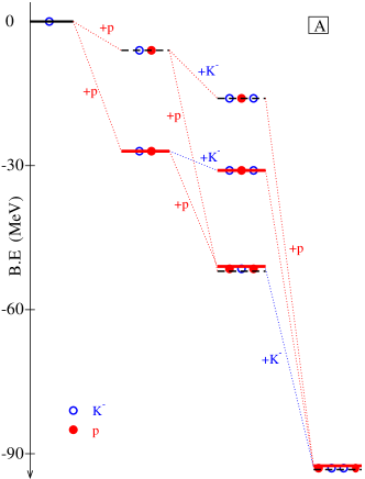
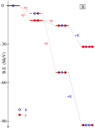
Figure 4: (Color online) Global view of the calculated bound-state energies $B.E$ (in MeV) of the kaonic nuclear systems, $\bar{K}N$, $\bar{K}NN$, $\bar{K}\bar{K}N$ and $\bar{K}\bar{K}NN$. Diagram (A) shows a comparison between the present calculations using one-pole version of the SIDDHARTA potential $V^{SIDD,One-pole}_{\bar{K}N-\pi\Sigma}$ (black dashed lines) and the results by Maeda et al. using a simple one-channel real potential for the $\bar{K}N$ interaction  maeda (red solid lines). Diagram (B) shows a comparison of the present calculations using the same potential in diagram (A) with the chiral-based results by Barnea et al. gal (red solid lines).

Solution of the Faddeev AGS equations corresponding to the bound and resonance states in the $(I,J^{\pi})=(\frac{1}{2},0^{-})$ and $(\frac{1}{2},\frac{1}{2}^{+})$ states of the $\bar{K}NN-\pi\Sigma{N}$ and $\bar{K}\bar{K}N-\bar{K}\pi\Sigma$ three-body systems, respectively, and $(I,J^{\pi})=(0,0^{+})$ state of $\bar{K}\bar{K}NN$ four-body system are found by applying search procedures described in sect. II. One- and two-pole version of the $\bar{K}N-\pi\Sigma$ interaction are considered and the dependence of the resulting few-body pole energy on the two-body $\bar{K}N-\pi\Sigma$ potentials is investigated. The $s$-wave (3+1) and (2+2) sub-amplitudes are obtained by using the Hilbert-Schmidt expansion (HSE) procedure for the integral kernels.

The calculated binding energies and the widths of the quasi-bound state of the $K^{-}pp$, $K^{-}K^{-}p$ and $K^{-}K^{-}pp$ systems for one- and two-pole of potentials are presented in table 3. The quasi-bound state position of the $K^{-}K^{-}pp$ system is obtained by keeping four terms ($N_{r}=4$) in the Hilbert-Schmidt expansion of the amplitudes (8) and (19), which will be suitable for practical calculations kh . It can be seen from table 3 that our calculated binding energies are very close to the other results obtained in revai and shev5 for $K^{-}pp$ and $K^{-}K^{-}p$ systems using the same $\bar{K}N-\pi\Sigma$ potentials within the coupled-channel Faddeev approach.

In the present calculations, the $\pi\bar{K}\Sigma{N}$ and $\pi\pi\Sigma\Sigma$ channels have not been included directly and one-channel Faddeev AGS equations are solved for the $\bar{K}\bar{K}NN$ system. We approximated the full coupled-channel one- and two-pole models of interaction by constructing the so-called exact optical $\bar{K}N-\pi\Sigma$ potential. The exact optical potential provides exactly the same elastic $\bar{K}N$ scattering amplitude as the coupled-channel model of interaction shev4 . Thus, our coupled-channels four-body calculations with coupled-channel $\bar{K}N-\pi\Sigma$ interaction is equivalent to the one-channel four-body calculation using the so-called exact optical $\bar{K}N(-\pi\Sigma)$ potential. The decaying to the $\pi\bar{K}\Sigma{N}$ and $\pi\pi\Sigma\Sigma$ channels is taken into account through the imaginary part of the optical $\bar{K}N(-\pi\Sigma)$ potential. The binding energy and width of the deeply bound dibaryonic double-$\bar{K}$ system, $K^{-}K^{-}pp$, is calculated as a natural extension of $K^{-}pp$ and $K^{-}K^{-}p$ systems. The last row for each potential in table 3 reports on the $K^{-}K^{-}pp$ quasi-bound state ($S=-2$) which has been highlighted as a possible doorway to kaon condensation in self-bound systems, given its large binding energy over 100 MeV predicted by Yamazaki et al. yamaz . The $K^{-}K^{-}pp$ system is tightly bound and has a larger binding energy than $K^{-}pp$, $B_{K^{-}K^{-}pp}\sim$80-94 MeV, and a width, $\Gamma=5-31$ MeV. In particular, it should be noted that the addition of one nucleon to the $K^{-}K^{-}p$ system gains $\sim$55-75 MeV, and the addition of one $\bar{K}$ to the $K^{-}pp$ system gains $\sim$35-40 MeV to the ground-state energy.

Table 3: The sensitivity of the pole position (in MeV), $z^{pole}_{X}$, of the quasi-bound states in $\bar{K}N$, $\bar{K}NN$, $\bar{K}\bar{K}N$ and $\bar{K}\bar{K}NN$ systems to the different models of $\bar{K}N-\pi\Sigma$ interaction. The real part of the pole position for each state is measured from the threshold of the corresponding kaonic system. $V^{One-pole}_{\bar{K}N-\pi\Sigma}$ and $V^{Two-pole}_{\bar{K}N-\pi\Sigma}$ standing for a one-pole and a two-pole structure of the $\Lambda$(1405) resonance.

	$V^{One-pole}_{\bar{K}N-\pi\Sigma}$	$V^{Two-pole}_{\bar{K}N-\pi\Sigma}$
With SIDD potential shev3 :
$z^{pole}_{\bar{K}N}$	$1428.1-i46.6$	$1418.1-i56.9$
		$1382.0-i104.2$
$z^{pole}_{\bar{K}NN}$	$-52.8-i31.5$	$-48.5-i24.1$
$z^{pole}_{\bar{K}\bar{K}N}$	$-17.8-i56.7$	$-27.6-i41.2$
$z^{pole}_{\bar{K}\bar{K}NN}$	$-92.7-i15.5$	$-83.8-i4.0$
With KEK potential shev4 :
$z^{pole}_{\bar{K}N}$	$1411.3-i35.8$	$1410.8-i35.9$
		$1380.8-i104.8$
$z^{pole}_{\bar{K}NN}$	$-44.5-i26.0$	$-45.9-i19.5$
$z^{pole}_{\bar{K}\bar{K}N}$	$-27.5-i38.1$	$-26.7-i30.6$
$z^{pole}_{\bar{K}\bar{K}NN}$	$-83.1-i12.4$	$-81.5-i2.3$

In order to investigate the importance of repulsion between two kaons in double-$\bar{K}$ systems, we looked at the dependence of $K^{-}K^{-}p$ and $K^{-}K^{-}pp$ binding energies on the repulsive $K^{-}K^{-}$ interaction. In table 4, the $K^{-}K^{-}p$ and $K^{-}K^{-}pp$ binding energies for different representative sets of $\bar{K}N-\pi\Sigma$ potentials are obtained when the repulsive $V^{I=1}_{\bar{K}\bar{K}}$ is taken to be zero. It can be seen from the tables 3 and 4 that while the presence and absence of the repulsive $K^{-}K^{-}$ interaction can change the binding energy of the $K^{-}K^{-}p$ system about 5-10 MeV, the variation of the binding energy in the case of the $K^{-}K^{-}pp$ system is very small for all $\bar{K}N$ interaction models. Therefore, in contrast to $K^{-}K^{-}p$ system, the s-wave $K^{-}K^{-}$ interaction, which is used in the present calculation, plays a minor role in the $K^{-}K^{-}pp$ binding energy. Most likely, it is caused by the relative weakness of the $K^{-}K^{-}$ interaction as compared to $\bar{K}N$ from the viewpoint of a deep quasi-bound in the latter system ($B.E_{\bar{K}N}\sim 6-25$ MeV).

Table 4: Pole positions, $z^{pole}_{X}$, of the quasi-bound states in $\bar{K}\bar{K}N$ and $\bar{K}\bar{K}NN$. In these calculations, the $\bar{K}\bar{K}$ interaction is turned off ($\tau^{I=1}_{\bar{K}\bar{K}}=0$). The real part of the pole position for each state is measured from the threshold of the corresponding system. Comparing the present results with those in table 3 shows that the binding energy of the $\bar{K}\bar{K}N$ system exhibits more sensitivity to the repulsive $\bar{K}\bar{K}$ interaction than the binding energy of the $\bar{K}\bar{K}NN$ four-body system.

$\bar{K}N$ interaction	$z^{pole}_{\bar{K}\bar{K}N}$ (MeV)	$z^{pole}_{\bar{K}\bar{K}NN}$
$V^{SIDD,One-pole}_{\bar{K}N-\pi\Sigma}$ shev3	$-27.9-i55.1$	$-93.7-i15.3$
$V^{KEK,One-pole}_{\bar{K}N-\pi\Sigma}$ shev4	$-33.2-i37.9$	$-84.6-i12.1$
$V^{SIDD,Two-pole}_{\bar{K}N-\pi\Sigma}$ shev3	$-32.0-i35.9$	$-84.2-i3.9$
$V^{KEK,Two-pole}_{\bar{K}N-\pi\Sigma}$ shev4	$-30.4-i27.2$	$-81.8-i2.3$

Recently, some few-body calculations are performed on the lightest kaonic nuclei by the hyperspherical harmonics gal and the Faddeev method maeda . Barnea et al. gal made a hyperspherical harmonics calculation for four-body $K^{-}K^{-}pp$ nuclear quasi-bound state using an energy dependent chiral interaction model for $\bar{K}N$ interaction. In this calculation, a quasi-bound state with $I=0$ and $J^{\pi}=0^{+}$, was found with a binding energy about 32 MeV and a width of 80 MeV below the threshold energy of the $\bar{K}\bar{K}NN$ state. However, their results were criticized in ref. revai . A similar conclusion was also drawn by Maeda et al. maeda using a simple one-channel real potential for the $\bar{K}N$ interaction combined with the Faddeev-Yakubowsky method. The obtained binding energy for the $\bar{K}\bar{K}NN$ was about 93 MeV below threshold energy. Our results for binding energy values of the $K^{-}pp$, $K^{-}K^{-}p$ and $K^{-}K^{-}pp$ quasi-bound state are compared with other theoretical results in fig. 4. The results obtained in Faddeev calculation using the one-pole version of the $\bar{K}N-\pi\Sigma$ potential $V^{SIDD,One-pole}_{\bar{K}N-\pi\Sigma}$ are shown together with Faddeev results in maeda (Diagram A) and variational results gal (Diagram B). It is seen from fig. 4 (Diagram B) that the energy dependent chiral $\bar{K}N$ potential leads to a more shallow quasi-bound state than the phenomenological one in three- and four-body systems. This is due to the energy dependence of the chiral potential. The comparison of our results for $\bar{K}\bar{K}NN$ obtained for PEST $NN$ interaction and the coupled-channel $\bar{K}N-\pi\Sigma$ interaction with standard binding energies calculated in ref. maeda within the Faddeev-Yakubowsky method for rank-two $NN$ interaction and one-channel real $\bar{K}N$ interaction shows that they are in the same order of magnitude (Diagram A). Although the present results for the quasi-bound states in the $K^{-}pp$ and $K^{-}K^{-}pp$ systems and the binding energies reported by Maeda et al. are in the same range, but this agreement seems to be rather accidental. We want to emphasize that in fact it is difficult to compare our results with those in Maeda et al. maeda . Firstly, as already said in the sect. III, the potential that we used here for the $\bar{K}N-\pi\Sigma$ interaction are adjusted to reproduce the experimental data on kaonic hydrogen and low-energy $K^{-}p$ scattering, but Maeda et al. maeda fixed the two-body energy arbitrarily to define the parameters of the $\bar{K}N$ potential. Secondly, in ref. maeda the $\pi\Sigma$ channel has not been included. The $\pi\Sigma$ channel plays an important dynamical role in forming the three- and four-body quasi-bound state. Thus, it is expected that the inclusion of $\pi\Sigma$ channel will have a serious effect on their obtained binding energy for $K^{-}pp$ and $K^{-}K^{-}pp$ quasi-bound states.

V Conclusion

In the present paper, non-relativistic four-body Faddeev equations have been applied to study the $\bar{K}\bar{K}NN$ system. The calculation scheme, which formally allows an exact solution, is based on the separable approximation of the appropriate integral kernels. We employed HSE method to reduce the problem to a set of single-variable integral equations. To investigate the dependence of the resulting four-body binding energy on models of $\bar{K}N-\pi\Sigma$ interaction, different versions of $\bar{K}N-\pi\Sigma$ potentials, which produce the one- or two-pole structure of $\Lambda$(1405) resonance, were used. We have also found that $K^{-}$-$K^{-}$ repulsion inside $K^{-}K^{-}pp$ in contrast to $K^{-}K^{-}p$ system, gives only a small effect on its binding energy and width, which does not alter the dense nature of this double- $\bar{K}$ cluster. The calculations yielded binding energies $B_{K^{-}pp}\sim$ 45-53, $B_{K^{-}K^{-}p}\sim$ 17-28 and $B_{K^{-}K^{-}pp}\sim$ 80-94 MeV for $K^{-}pp$, $K^{-}K^{-}p$ and $K^{-}K^{-}pp$ systems, respectively. The obtained widths for these systems are $\Gamma_{K^{-}pp}\sim$ 40-62, $\Gamma_{K^{-}K^{-}p}\sim$ 60-110 and $\Gamma_{K^{-}K^{-}pp}\sim$ 5-31 MeV. The calculations suggest that few-body double-$\bar{K}$ nuclei, such as $K^{-}K^{-}pp$, as well as single-$\bar{K}$ nuclei, are tightly bound systems with large binding energies. The results of the one-channel AGS calculations of $K^{-}K^{-}pp$ show that, if the difference between the two sets of the $K^{-}K^{-}pp$ binding energies corresponding to the one- and two-pole versions of the coupled-channel $\bar{K}N-\pi\Sigma$ potential is much more than theoretical uncertainties, then it would be possible to favor one version of $\bar{K}N-\pi\Sigma$ potential by comparing with an experimental result. Similar calculations could be performed for the chiraly motivated $\bar{K}N$ input potential, too. The quasi-bound states resulting from the energy-dependent potentials happen to be shallower because of the weaker $\bar{K}N$ attraction for lower energies than the energy independent potentials under consideration in this work.

The authors are thankful to A. Fix for his helpful discussions. The authors also gratefully acknowledge the Sheikh Bahaei National High Performance Computing Center (SBNHPCC) for providing computing facilities and time. SBNHPCC is supported by the scientific and technological department of presidential office and Isfahan University of Technology (IUT).

References

- (1) Y. Akaishi and T. Yamazaki, Phys. Rev. C 65, 044005 (2002).
- (2) T. Yamazaki and Y. Akaishi, Phys. Lett. B 535, 70 (2002).
- (3) A. Dote, H. Horiuchi, Y. Akaishi and T. Yamazaki, Phys. Lett. B 590, 51 (2004).
- (4) A. Dote, H. Horiuchi, Y. Akaishi and T. Yamazaki, Phys. Rev. C 70, 044313 (2004).
- (5) N. V. Shevchenko, A. Gal and J. Mares, Phys. Rev. Lett. 98, 082301 (2007).
- (6) N. V. Shevchenko, A. Gal, J. Mares and J. Revai, Phys. Rev. C 76, 044004 (2007).
- (7) J. Revai and N. V. Shevchenko, Phys. Rev. C 90, 034004 (2014).
- (8) Y. Ikeda and T. Sato, Phys. Rev. C 76, 035203 (2007).
- (9) Y. Ikeda and T. Sato, Phys. Rev. C79, 035201 (2009).
- (10) Y. Ikeda, H. Kamano and T. Sato, Prog. Theor. Phys. 124, 533 (2010).
- (11) S. Maeda, Y. Akaishi and T. Yamazaki, Proc. Jpn. Acad., Ser. B 89, 418 (2013).
- (12) M. Agnello, et al., Phys. Rev. Lett. 94, 212303 (2005).
- (13) T. Yamazaki, et al., Phys. Rev. Lett. 104, 132502 (2010).
- (14) T. Yamazaki and Y. Akaishi, Proc. Jpn. Acad., Ser. B 83, 144 (2007).
- (15) T. Yamazaki and Y. Akaishi, Phys. Rev. C 76, 045201 (2007).
- (16) Y. Ichikawa, et al., Prog. Theor. Exp. Phys. 021D01, (2015).
- (17) T. Hiraiwa, et al., Int. J. Mod. Phys. A 26, 561 (2011).
- (18) N. V. Shevchenko and J. Haidenbauer, Phys. Rev. C 92, 044001 (2015).
- (19) Yoshiko Kanada-En’yo and Daisuke Jido, Phys. Rev. C 78, 025212 (2008).
- (20) T. Yamazaki, A. Dote and Y. Akaishi, Phys. Lett. B 587, 167 (2004).
- (21) D. B. Kaplan and A. E. Nelson, Phys. Lett. B 175, 57 (1986).
- (22) P. Grassberger and W. Sandhas, Nucl. Phys. B 2, 181 (1967).
- (23) I. M. Nadrodetsky, Nucl. Phys. A 221, 191 (1974).
- (24) S. A. Sofianos, N. J. McGurk, and H. Fiedeldey, Nucl. Phys. A 318, 295 (1979).
- (25) N. V. Shevchenko, Nucl. Phys. A 890-891, 50 (2012).
- (26) N. V. Shevchenko, Phys. Rev. C 85, 034001 (2012).
- (27) S. R. Beane et al., (NPLQCD Collaboration), Phys. Rev. D 77, 094507 (2008).
- (28) E. O. Alt, P. Grassberger, and W. Sandhas, Phys. Rev. C 1, 85 (1970).
- (29) O. A. Yakubovsky, Yad. Fiz. 5, 1312 (1967) (Trans.: Sov. J. Nucl. Phys. 5, 937 (1967)).
- (30) L. D. Faddeev, Proc. First Int. Conf. on the Three-Body Problem, Birmingham, 1969, eds. J.S.C. McKee and P.M. Rolph (North-Holland, Amsterdam 1970).
- (31) A. C. Fonseca, Proc. 8th Autumn School on Models and Methods in Few-Body Physics, Lisboa, 1986, eds. L.S. Ferreira, A.C. Fonseca and L. Streit, Lecture Notes in Physics 273, 161 (1986).
- (32) M. Bazzi, et al., (SIDDHARTA collaboration), Phys. Lett. B 704, 113 (2011).
- (33) M. Iwasaki, et al., Phys. Rev. Lett. 78, 3067 (1997).
- (34) T. M. Ito et al., Phys. Rev. C 58, 2366 (1998).
- (35) H. Zankel, W. Plessas and J. Haidenbauer, Phys. Rev. C 28, 538 (1983).
- (36) M. Torres, R. H. Dalitz, and A. Deloff, Phys. Lett. B 174, 213 (1986).
- (37) S. Marri and S. Z. Kalantari, Eur. Phys. J. A 52, 282 (2016).
- (38) N. Barnea, A. Gal and E. Z. Liverts, Phys. Lett. B 712, 132 (2012).