The role of volume and surface spontaneous parametric down-conversion in the generation of photon pairs in layered media

Abstract

A rigorous description of volume and surface spontaneous parametric down-conversion in 1D nonlinear layered structures is developed considering exact continuity relations for the fields’ amplitudes at the boundaries. The nonlinear process is described by the quantum momentum operator that provides the Heisenberg equations which solution is continuous at the boundaries. The transfer-matrix formalism is applied. The volume and surface contributions are clearly identified. Numerical analysis of a structure composed of 20 alternating GaN/AlN layers is given as an example.

I Introduction

Spontaneous parametric down-conversion (SPDC) is a second-order nonlinear process Louisell et al. (1961); Harris et al. (1967); Magde and Mahr (1967) in which one photon with higher energy is annihilated and two photons of lower energies are simultaneously created. Due to the laws of energy and momentum conservations quantum correlations (entanglement) between the photons in a pair emerge Keller and Rubin (1997); Svozilík et al. (2012); Grice et al. (2008); Javůrek et al. (2014). The process of SPDC occurs either inside the media with non-zero second-order permittivity tensor (non-centrosymmetric crystals) or at the boundaries of these media Peřina Jr. et al. (2009a); Peřina Jr. (2014); Boyd (2003).

The process of SPDC has been observed in nonlinear bulk media Boyd (2003); Dmitriev et al. (1999), systems of nonlinear thin layers Peřina Jr. et al. (2006, 2009b); Peřina Jr. (2011) including metallo-dielectric layers Javůrek et al. (2014); Javurek et al. (2012, 2014), nonlinear photonic fibers Zhu et al. (2012); Javůrek et al. (2014a, 2014), nonlinear photonic waveguides Eckstein et al. (2011); Jachura et al. (2014); Machulka et al. (2013); Clausen et al. (2014), as well as in complex nonlinear photonic structures Chen et al. (2014). Bulk media including the most common nonlinear crystals LiNbO₃ and KTP represent the historically oldest sources of photon pairs. Periodically-poled nonlinear crystals with their freedom in tailoring phase-matching conditions have been obtained later, at the beginning of the 90’s Hayata and Koshiba (1991). At the same time periodically poled waveguides Lim et al. (1989); Shinozaki et al. (1992) and fibers Kashyap (1991); Chmela (1991) followed them up.

In the process of SPDC in homogeneous bulk media, phase matching of all three interacting fields (pump, signal and idler) in the direction of their propagation as well as in their transverse planes is needed to arrive at efficient nonlinear interaction. Phase-matching conditions can be achieved by angle or temperature tuning of birefringent crystals Boyd (2003). Or, alternatively, by poling a nonlinear crystal Harris (2007); Brida et al. (2009); Svozilík and Peřina Jr. (2009, 2011) which results in quasi-phase-matching conditions. However, if the length of a nonlinear medium is comparable to the interacting fields’ wavelengths, the phase-matching condition does not play an important role in reaching efficient nonlinear interaction. Instead, the overlap of electric-field amplitudes of the interacting fields inside the medium is crucial. Moreover, the contribution of the nonlinear interaction around the boundaries of such thin media becomes important Bloembergen and Pershan (1962); Bloembergen et al. (1969); Mlejnek et al. (1999); Centini et al. (2008). Provided that the number of boundaries per unit length (or volume) of the crystal (photonic structure) is sufficiently high, the emission rate of photon pairs coming from the boundaries may even be comparable to the emission rate of photon pairs created in the volume Peřina Jr. et al. (2009c). This also concerns the nonlinear poled structures in which the boundaries are formed inbetween the domains with different signs of $\chi^{(2)}$ susceptibility.

Theoretical approaches to SPDC in layered structures (including poled crystals) have been developed in the Schrödinger as well as the Heisenberg pictures. In the Schrödinger picture, a perturbation solution of the Schrödinger equation in the nonlinear coupling constant was found. In the first order, it describes the generation of one photon pair Peřina Jr. (2011); Javurek et al. (2012); Javůrek et al. (2014b). On the other hand, linear Heisenberg equations occur in the Heisenberg picture. They allow to treat the nonlinear interaction for arbitrarily intense signal and idler fields. Their solution can also be conveniently written such that the continuity requirements of the electric- and magnetic-field operator amplitudes at the boundaries are fulfilled. This allows to describe simultaneously the volume and surface contributions to SPCD.

Using the Heisenberg picture, the volume contribution to SPDC has been widely studied in Refs. Huttner et al. (1990); Ben-Aryeh and Serulnik (1991); Peřina Jr. (2011) whereas the emission of photon pairs at the boundaries has been treated in Ref. Peřina Jr. et al. (2009c) applying the perturbation technique. The perturbation approach allowed to introduce corrections to the creation and annihilation operators of the signal and idler fields independently and then to apply the transfer-matrix formalism. Contrary to this, the theory developed here treats the fields at the boundaries in general which results in the coupling between the signal- and idler-field operators analyzed first in Ref. Lukš et al. (2012); Peřinová et al. (2013) for the cw-interaction. This means that the developed theory is more general (and more precise) compared to that of Ref. Peřina Jr. et al. (2009c), though it requires an extensive numeric approach. Moreover, it clearly identifies the fields arising in the volume and surface SPDC.

The paper is structured as follows. In Sec. II, the model describing both volume and surface SPDC is developed. In Sec. III, quantities characterizing photon pairs and derived from the general solution are defined. Results of numerical simulations are discussed in Sec. IV. Conclusions are drawn in Sec. V.

II Volume and surface spontaneous parametric down-conversion

The proposed model of SPDC is appropriate for 1D nonlinear photonic structures composed of parallel layers (or domains) having in general different material parameters and lengths. As an example, we consider a layered structure composed of alternating layers with different linear indices of refraction and nonlinear susceptibilities (see Fig. 1).

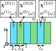
Figure 1: [Color online] Scheme of a layered structure. Second-order tensor $\boldsymbol{\chi}^{(2)(l)}$ of nonlinear susceptibility characterizes an $l$-th layer with index $n^{(l)}(\omega)$ of refraction; $L_{l}$ is the length of the $l$-th layer and $z_{l}$ ($z_{l+1}$) denotes the position of its left (right) boundary.

The process of SPCD is assumed to be pumped by a strong (un-depleted) classical field. In a layered structure, the positive-frequency vectorial electric-field amplitude $\mathbf{E}_{\rm p}^{(+)}(z,t)$ of the pump beam can conveniently be decomposed as follows Peřina Jr. (2011); Peřina Jr. et al. (2009c):

$$\mathbf{E}_{\rm p}^{(+)}(z,t)= \int_{0}^{\infty}d\omega_{\rm p}\sum_{l=0}^{N+1}\mathrm{rect}^{(l)}(z)\sum_{g={\rm F,B}}^{\gamma={\rm x,y}}\mathbf{e}_{{\rm p},\gamma}A_{{\rm p}_{g},\gamma}^{(l)}(\omega_{\rm p})$$

$$\times\mathrm{exp}\left[ik^{(l)}_{{\rm p}_{g},\gamma}(\omega_{\rm p})(z-z_{l})-i\omega_{\rm p}t\right];$$ (1)

$\omega_{\rm p}$ denotes the angular frequency of the pump beam. Function $\mathrm{rect}^{(l)}(z)$ is nonzero only for $z\in(z_{l},z_{l+1})$ where $\mathrm{rect}^{(l)}(z)=1$, $l\in\{1,\ldots,N\}$. For the input [output] medium, we have $\mathrm{rect}^{(0)}(z)=1$ for $z\in(-\infty,z_{1})$ [$\mathrm{rect}^{(N+1)}(z)=1$ for $z\in(z_{N+1},\infty)$] and it equals zero otherwise. Amplitude $A_{{\rm p}_{g},\gamma}^{(l)}$ occurring in Eq. (1) denotes the spectral pump electric-field amplitude at the left boundary of an $l$-th layer. The forward- (backward-) propagating fields are indicated by index ${\rm F}$ (${\rm B}$). The unit electric-field vectors $\mathbf{e}_{{\rm p},\gamma}$ determine the field’s polarization either along the ${\rm x}$ or ${\rm y}$ axis Yeh (1988); Peřina Jr. (2011, 2014). The wave numbers $k_{{\rm p}_{g},\gamma}^{(l)}$ satisfy the linear dispersion relations appropriate to an $l$-th layer, $k^{(l)}_{{\rm p}_{g},\gamma}(\omega_{\rm p})=\pm(\omega_{\rm p}/c)n_{{\rm p},\gamma}^{(l)}(\omega_{\rm p})$, $c$ being the speed of light in vacuum and $n_{{\rm p},\gamma}^{(l)}(\omega_{\rm p})$ denoting index of refraction in this layer. The plus (minus) sign in the definition of $k^{(l)}_{{\rm p}_{g},\gamma}$ refers to the forward- (backward-) propagating field. Symbol $\sum_{g}^{\gamma}$ stands for the summation over both the direction of field’s propagation and polarization.

The signal and idler positive-frequency vectorial electric-field operator amplitudes $\hat{\mathbf{E}}^{(+)}_{\rm s}(z,t)$ and $\hat{\mathbf{E}}^{(+)}_{\rm i}(z,t)$, respectively, are defined similarly as the pump amplitude:

$$\hat{\mathbf{E}}^{(+)}_{m}(z,t) = i\int_{0}^{\infty}d\omega_{m}\sum_{l=0}^{N+1}\tau_{m,\alpha}^{(l)}(\omega_{m})\mathrm{rect}^{(l)}(z)\sum_{a={\rm F,B}}^{\alpha={\rm x,y}}$$ (2)

$$\mathbf{e}_{m,\alpha}\hat{a}^{(l)}_{m_{a},\alpha}(z,\omega_{m})\mathrm{exp}\left(-i\omega_{m}t\right);\hskip 14.22636ptm\in\{{\rm s,i}\}.$$

In Eq. (2), amplitude $\tau_{m,\alpha}^{(l)}(\omega_{m})$ per one photon is defined as

$$\tau^{(l)}_{m,\alpha}(\omega_{m})=\sqrt{\frac{\hbar\omega_{m}}{4\pi\varepsilon_{0}cn_{m,\alpha}^{(l)}(\omega_{m})A}}$$ (3)

assuming homogeneous fields localized in transverse area $A$. Symbols $\mathbf{e}_{m,\alpha}$ introduced in Eq. (3) denote the unit polarization vectors in field $m$ and $\hbar$ stands for the reduced Planck constant. Operator $\hat{a}^{(l)}_{m_{a},\alpha}(z,\omega_{m})$ annihilates one photon at position $z$ in field $m$ propagating in direction $a$ with polarization $\alpha$ and frequency $\omega_{m}$. The annihilation operator $\hat{a}^{(l)}_{m_{a},\alpha}(z,\omega_{m})$ is assumed to fulfill the equal-space commutation relations together with its hermitian conjugated creation operator $\hat{a}^{(l)\dagger}_{m_{a},\alpha}(z,\omega_{m})$: Huttner et al. (1990); Ben-Aryeh and Serulnik (1991); Peřina Jr. et al. (2009c)

$$[\hat{a}^{(l)}_{m_{a},\alpha}(z,\omega_{m}),\hat{a}^{(l)\dagger}_{m^{\prime}_{a^{\prime}},\alpha^{\prime}}(z,\omega_{m}^{\prime})] = \delta_{aa^{\prime}}\delta_{mm^{\prime}}\delta_{\alpha\alpha^{\prime}}$$ (4)

$$\times\delta(\omega_{m}-\omega_{m}^{\prime}).$$

Spatial evolution of the operator $\hat{a}^{(l)}_{m_{a},\alpha}(z,\omega_{m})$ is given by the Heisenberg equation

$$\frac{\partial\hat{a}^{(l)}_{m_{a},\alpha}}{\partial z}(z,\omega_{m})=\frac{1}{i\hbar}[\hat{G}_{z}(z),\hat{a}^{(l)}_{m_{a},\alpha}(z,\omega_{m})]$$ (5)

derived from the following momentum operator $\hat{G}_{z}$ Ben-Aryeh and Serulnik (1991):

$$\hat{G}_{z}(z) = A\int_{-\infty}^{\infty}dt\,\hat{\sigma}_{\rm zz}^{\mathrm{eff}}(z,t),$$ (6)

$$\hat{\sigma}_{\rm zz}^{\mathrm{eff}}(z,t) = \sum_{m={\rm s,i}}\sum_{a={\rm F,B}}^{\alpha={\rm x,y}}\Bigl{\{}\varepsilon_{0}\hat{\mathbf{E}}_{m_{a},\alpha}^{(-)}(z,t)\cdot\hat{\mathbf{E}}_{m_{a},\alpha}^{(+)}(z,t)$$

$$+\frac{1}{\mu_{0}}\hat{\mathbf{B}}_{m_{a},\alpha}^{(-)}(z,t)\cdot\hat{\mathbf{B}}_{m_{a},\alpha}^{(+)}(z,t)$$

$$+\varepsilon_{0}\int_{0}^{\infty}d\omega_{m}\int_{0}^{\infty}d\omega_{m}^{\prime}\,\chi^{(1)}(\omega_{m})$$

$$\Bigl{.}\times\hat{\mathbf{E}}_{m_{a},\alpha}^{(-)}(z,\omega_{m}^{\prime})\cdot\hat{\mathbf{E}}_{m_{a},\alpha}^{(+)}(z,\omega_{m})\mathrm{exp}[-i(\omega_{m}-\omega_{m}^{\prime})t]\Bigr{\}}$$

$$+2\varepsilon_{0}\int_{0}^{\infty}d\omega_{\rm p}\int_{0}^{\infty}d\omega_{\rm s}\int_{0}^{\infty}d\omega_{\rm i}\,\boldsymbol{\chi}^{(2)}(\omega_{\rm p};\omega_{\rm s},\omega_{\rm i})\mathbf{:}\mathbf{E}_{\rm p}(z,\omega_{\rm p})$$

$$\times\hat{\mathbf{E}}_{\rm s}^{\dagger}(z,\omega_{\rm s})\hat{\mathbf{E}}_{\rm i}^{\dagger}(z,\omega_{\rm i})\mathrm{exp}\left[-i(\omega_{\rm p}-\omega_{\rm s}-\omega_{\rm i})t\right].$$

In Eq. (LABEL:e7), $\hat{\sigma}_{\rm zz}^{\mathrm{eff}}$ means the ${\rm zz}$ component of effective Maxwell stress-tensor operator and $\hat{\mathbf{E}}^{(+)}_{m_{a},\alpha}(z,\omega_{a})$ stands for the spectral positive-frequency electric-field operator amplitude [$\hat{\mathbf{E}}^{(+)}_{m}(z,t)=\sum_{a={\rm F,B}}^{\alpha={\rm x,y}}\int_{0}^{\infty}d\omega_{a}\,\hat{\mathbf{E}}^{(+)}_{m_{a},\alpha}(z,\omega_{a})\,\mathrm{exp}(-i\omega_{a}t)$]. Spectral positive-frequency magnetic-field operator amplitudes $\hat{\mathbf{B}}^{(+)}_{m_{a},\alpha}(z,\omega_{m})$ are derived from the Maxwell equations [$\hat{\mathbf{B}}^{(+)}_{m_{a},{\rm y}}(z,\omega_{m})=\mathbf{k}_{m,\alpha}(\omega_{m})\times\hat{\mathbf{E}}^{(+)}_{m_{a},{\rm x}}(z,\omega)/\omega_{m}$]. Symbol $\cdot$ denotes scalar product and operation $\boldsymbol{:}$ shorthands tensor $\boldsymbol{\chi}^{(2)}$ with respect to its three indices.

Applying Eqs. (1), (2), (6), and (LABEL:e7) the following explicit form of momentum operator $\hat{G}_{\rm z}(z)$ is obtained:

$$\hat{G}_{\rm z}(z)=\sum_{m={\rm s,i}}\sum_{l=0}^{N+1}\int_{0}^{\infty}d\omega_{m}\sum_{a={\rm F,B}}^{\alpha={\rm x,y}}\mathrm{rect}^{(l)}(z)\hbar k^{(l)}_{m,\alpha}(\omega_{m})$$

$$\times\hat{a}_{m_{a},\alpha}^{(l)\dagger}(z,\omega_{m})\hat{a}^{(l)}_{m_{a},\alpha}(z,\omega_{m})$$

$$-i\hbar\int_{0}^{\infty}d\omega_{\rm s}\int_{0}^{\infty}d\omega_{\rm i}\sum_{a,b,g={\rm F,B}}^{\alpha,\beta,\gamma={\rm x,y}}\sum_{l=1}^{N}T_{g}^{\alpha\beta\gamma,(l)*}(\omega_{\rm s},\omega_{\rm i})$$

$$\times\exp\left[ik_{{\rm p}_{\gamma},g}^{(l)}(\omega_{\rm s}+\omega_{\rm i})(z-z_{l})\right]\hat{a}^{(l)\dagger}_{{\rm s}_{a},\alpha}(z,\omega_{\rm s})\hat{a}^{(l)\dagger}_{{\rm i}_{b},\beta}(z,\omega_{\rm i})$$

and

$$T^{\alpha\beta\gamma,(l)}_{g}(\omega_{\rm s},\omega_{\rm i})\equiv\frac{4i\pi\varepsilon_{0}A}{\hbar}\tau_{{\rm s},\alpha}^{(l)}(\omega_{\rm s})\tau_{{\rm i},\beta}^{(l)}(\omega_{\rm i})$$

$$\times\boldsymbol{\chi}^{(2)(l)}(\omega_{\rm s}+\omega_{\rm i};\omega_{\rm s},\omega_{\rm i})\mathbf{:}\mathbf{e}_{{\rm p},\gamma}\mathbf{e}_{{\rm s},\alpha}\mathbf{e}_{{\rm i},\beta}A^{(l)*}_{{\rm p}_{g},\gamma}(\omega_{\rm s}+\omega_{\rm i}).$$

Symbol $k_{m,\alpha}^{(l)}$ occurring in Eq. (LABEL:e8) denotes the absolute value of wave vector $k_{m_{a},\alpha}^{(l)}$. Below, we utilize the formalism that does not distinguish explicitly between the forward- and backward-propagating modes via the sign of wave vectors. Instead, appropriate signs are added to the linear and nonlinear terms in momentum operator $\hat{G}_{\rm z}$.

Applying the commutation relations (4) the Heisenberg equations (5) are obtained in their explicit form:

$$\frac{\partial\hat{a}_{{\rm s}_{a},\alpha}^{(l)}}{\partial z}(z,\omega_{\rm s}) = ik_{{\rm s}_{a},\alpha}^{(l)}\hat{a}_{{\rm s}_{a},\alpha}^{(l)}(z,\omega_{\rm s})+[\pm 1]_{a}\int_{0}^{\infty}d\omega_{\rm i}\,$$

$$\sum_{b,g={\rm F,B}}^{\beta,\gamma={\rm x,y}}T_{g}^{\alpha\beta\gamma,(l)*}(\omega_{\rm s},\omega_{\rm i})\exp[ik_{{\rm p}_{g},\gamma}^{(l)}(z-z_{l})]\hat{a}_{{\rm i}_{b},\beta}^{(l),\dagger}(z,\omega_{\rm i}).$$

Symbol $[\pm 1]_{a}$ equals $+1$ for a forward propagating field ($a={\rm F}$) and $-1$ for a backward propagating field ($a={\rm B}$).

The solution of Heisenberg equation (LABEL:e10b) for the signal-field operator $\hat{a}_{{\rm s}_{a},\alpha}^{(l)}$ consists of the homogeneous and particular solutions:

$$\hat{a}_{{\rm s}_{a},\alpha}^{(l)}(z,\omega_{\rm s}) = \hat{\bar{a}}^{(l)}_{{\rm s}_{a},\alpha}(z_{l},\omega_{\rm s})\exp[ik_{{\rm s}_{a},\alpha}^{(l)}(\omega_{\rm s})(z-z_{l})]$$ (11)

$$+\int_{0}^{\infty}d\omega_{\rm i}\sum_{b={\rm F,B}}^{\beta={\rm x,y}}\Phi_{s,ab}^{\alpha\beta,(l)*}(z,\omega_{\rm s},\omega_{\rm i})\,\hat{\bar{a}}_{{\rm i}_{b},\beta}^{(l)\dagger}(z_{l},\omega_{\rm i})$$

$$\times\exp[ik_{{\rm s}_{a},\alpha}^{(l)}(\omega_{\rm s})(z-z_{a}^{(l)})]$$

and

$$\Phi_{s,ab}^{\alpha\beta,(l)}(z,\omega_{\rm s},\omega_{\rm i}) \equiv i[\pm 1]_{a}\sum_{g={\rm F,B}}^{\gamma={\rm x,y}}T_{g}^{\alpha\beta\gamma,(l)}(\omega_{\rm s},\omega_{\rm i})$$ (12)

$$\times\mathrm{rect}^{(l)}(z)\exp[-i\phi_{{\rm s}_{a},bg}^{\beta\gamma,(l)}(\omega_{\rm s},\omega_{\rm i})]$$

$$\times\frac{\exp\left[-i\Delta k_{abg}^{\alpha\beta\gamma,(l)}(z-z_{a}^{(l)})\right]-1}{\Delta k_{abg}^{\alpha\beta\gamma,(l)}}.$$

We note that the particular solution has been derived by the convolution of the Green function of Eq. (LABEL:e10b) and the nonlinear source term on the right-hand side of Eq. (LABEL:e10b). The signal-field annihilation operator $\hat{\bar{a}}_{{\rm s}_{a},\alpha}^{(l)}(z_{l},\omega_{\rm s})$ and idler-field creation operator $\hat{\bar{a}}_{{\rm i}_{b},\beta}^{(l)\dagger}(z_{l},\omega_{\rm i})$ occurring at the right-hand side of Eq. (11) are appropriate for the homogeneous solution and so they describe the free-field propagation. Spatial dependence of the signal-field operator $\hat{\bar{a}}_{{\rm s}_{a},\alpha}^{(l)}(z,\omega_{\rm s})$, considered as an example, is thus described as

$$\hat{\bar{a}}_{{\rm s}_{a},\alpha}^{(l)}(z,\omega_{\rm s})=\hat{\bar{a}}_{{\rm s}_{a},\alpha}^{(l)}(z_{l},\omega_{\rm s})\exp[ik_{{\rm s}_{a},\alpha}^{(l)}(z-z_{l})].$$ (13)

The signal- and idler-field operators $\hat{\bar{a}}_{{\rm s}_{a},\alpha}^{(l)}(z,\omega_{\rm s})$ and $\hat{\bar{a}}_{{\rm i}_{b},\beta}^{(l)\dagger}(z,\omega_{\rm i})$ also obey the equal space commutation relations

$$[\hat{\bar{a}}_{m_{a},\alpha}^{(l)}(z,\omega_{m}),\hat{\bar{a}}_{{m^{\prime}}_{a^{\prime}},\alpha^{\prime}}^{(l)}(z,\omega_{m^{\prime}}^{\prime})] = \delta_{mm^{\prime}}\delta_{aa^{\prime}}\delta_{\alpha\alpha^{\prime}}$$ (14)

$$\times\delta(\omega_{m}-\omega_{m}^{\prime}).$$

In Eq. (12), the difference $\Delta k_{abg}^{\alpha\beta\gamma,(l)}$ of wave vectors in an $l$-th layer equals $\Delta k_{abg}^{\alpha\beta\gamma,(l)}=k_{{\rm p}_{g},\gamma}^{(l)}-k_{{\rm s}_{a},\alpha}^{(l)}-k_{{\rm i}_{b},\beta}^{(l)}$. Position $z_{a}^{(l)}$ in the $l$-th layer equals $z_{l}$ ($z_{l+1}$) for forward- (backward-) propagating fields. Similarly, phase factor $\phi_{{\rm s}_{a},bg}^{\beta\gamma,(l)}$ introduced in Eq. (12) is equal to zero [$k_{{\rm p}_{g},\gamma}^{(l)}-k_{{\rm i}_{b},\beta}^{(l)})L^{(l)}$] for forward- [backward-] propagating fields. The solution for the idler-field operators is derived from Eq. (11) invoking the symmetry between the signal and idler fields ($s\leftrightarrow i$).

The spatial dependence of signal [idler] electric-field operator amplitude $\hat{\mathbf{E}}_{\rm s}(z,t)$ [$\hat{\mathbf{E}}_{\rm i}(z,t)$] inside the structure is determined once we know the transformations between the signal [idler] operators $\hat{\bar{a}}_{{\rm s}_{a},\alpha}^{(l-1)}$ [$\hat{\bar{a}}_{{\rm i}_{b},\beta}^{(l-1)\dagger}$] and $\hat{\bar{a}}_{{\rm s}_{a},\alpha}^{(l)}$ [$\hat{\bar{a}}_{{\rm i}_{b},\beta}^{(l)\dagger}$] in all adjacent layers $l-1$ and $l$. The transformation is derived from the boundary conditions for the electric- and magnetic-field operators and the propagation formula (13). The boundary conditions for the signal-field operators between layers $l-1$ and $l$ require the continuity of electric- [$\hat{\mathbf{E}}_{\rm s}^{(l-1)}(z,t)$ and $\hat{\mathbf{E}}_{\rm s}^{(l)}(z,t)$] and magnetic-field [$\hat{\mathbf{H}}_{\rm s}^{(l-1)}(z,t)$ and $\hat{\mathbf{H}}_{\rm s}^{(l)}(z,t)$] vectorial operator amplitudes. Applying the field’s decomposition written in Eq. (2) the boundary conditions are transformed into the following relations:

$$\tau^{(l-1)}_{m,\alpha}(\omega_{m})\sum_{a={\rm F,B}}\hat{a}^{(l-1)}_{m_{a},\alpha}(z_{l},\omega_{m}) =$$ (15)

$$\tau^{(l)}_{m,\alpha}(\omega_{m})\sum_{a={\rm F,B}}\hat{a}^{(l)}_{m_{a},\alpha}(z_{l},\omega_{m}),$$

$$\tau^{(l-1)}_{m,\alpha}(\omega_{m})\sum_{a={\rm F,B}}\frac{\partial\hat{a}^{(l-1)}_{m_{a},\alpha}}{\partial z}(z_{l},\omega_{m}) =$$

$$\tau^{(l)}_{m,\alpha}(\omega_{m})\sum_{a={\rm F,B}}\frac{\partial\hat{a}^{(l)}_{m_{a},\alpha}}{\partial z}(z_{l},\omega_{m});\,\alpha\in\{{\rm x,y}\}.$$

The relations (15) and (LABEL:e32) assume that both ${\rm x}$ and ${\rm y}$ polarization vectors $\mathbf{e}_{m,\alpha}$ of the electric field [see Eq. (2)] preserve their orientation after reflection at the boundary. This definition is equivalent to that of the TE-polarized electric-field vector in the general linear transmission/reflection scheme Yeh (1988). We note that, in the analyzed 1D geometry, the TE- and TM-polarized waves are physically equivalent.

To allow for further manipulations with the above derived relations (and later the numerical treatment), we introduce suitable orthonormal bases $f_{{\rm s},k}(\omega_{\rm s})$ and $f_{{\rm i},k}(\omega_{\rm i})$, $k=0,\ldots,\infty$, in the signal and idler fields, respectively. This results in the replacement of ’continuous indices’ $\omega_{\rm s}$ and $\omega_{\rm i}$ by the discrete index $k$. In these bases, new signal [idler] field operators $\hat{A}_{{\rm s}_{a},\alpha,k}^{(l)}(z)$ [$\hat{A}_{{\rm i}_{b},\beta,k}^{(l)\dagger}(z)$] are defined as follows:

$$\hat{A}_{{\rm s}_{a},\alpha,k}^{(l)}(z) = \int_{0}^{\infty}d\omega_{\rm s}\,f_{{\rm s},k}^{*}(\omega_{\rm s})\,\hat{a}_{{\rm s}_{a},\alpha}^{(l)}(z,\omega_{\rm s}).$$ (17)

The original operators are obtained by the inverse transformation

$$\hat{a}_{{\rm s}_{a},\alpha}^{(l)}(z,\omega_{\rm s}) = \sum_{k=0}^{\infty}f_{{\rm s},k}(\omega_{\rm s})\hat{A}_{{\rm s}_{a},\alpha,k}^{(l)}(z).$$ (18)

Equations (15) and (LABEL:e32) can be conveniently rewritten into a matrix form. As the derivation procedure is similar for both equations, we focus here only on the transformation of Eq. (15) written for the signal field. The solution for signal-field operator $\hat{a}_{{\rm s}_{a},\alpha}^{(l)}(z_{l},\omega_{\rm s})$ given in Eq. (11) is inserted into Eq. (15) first. Then, introducing vectorial operators $\hat{\mathbf{A}}_{{\rm s}_{a},\alpha}^{(l)}$ and $\hat{\mathbf{A}}_{{\rm i}_{b},\beta}^{(l)\dagger}$ with the elements $[\hat{\mathbf{A}}_{{\rm s}_{a},\alpha}^{(l)}]_{k}=\hat{A}_{{\rm s}_{a},\alpha,k}^{(l)}$ and $[\hat{\mathbf{A}}_{{\rm i}_{b},\beta}^{(l)\dagger}]_{k}=\hat{A}_{{\rm i}_{b},\beta,k}^{(l)\dagger}$ the relations (15) for the continuity of electric-field amplitudes are expressed in the form:

$$\mathbf{I}_{E{\rm s},\alpha}^{(l-1)}\sum_{a={\rm F,B}}\hat{\mathbf{A}}_{{\rm s}_{a},\alpha}^{(l-1)}(z_{l})+\sum_{a,b={\rm F,B}}^{\beta={\rm x,y}}\mathbf{I}_{{\rm s},\alpha}^{(l-1)}\mathbf{J}_{E{\rm s},ab}^{\alpha\beta,(l-1)}(z_{l})$$

$$\times\hat{\mathbf{A}}_{{\rm i}_{b},\beta}^{(l-1)\dagger}(z_{l})=\mathbf{I}_{E{\rm s},\alpha}^{(l)}\sum_{a={\rm F,B}}\hat{\mathbf{A}}_{{\rm s}_{a},\alpha}^{(l)}(z_{l})+\sum_{a,b={\rm F,B}}^{\beta={\rm x,y}}\mathbf{I}_{{\rm s},\alpha}^{(l)}$$

$$\times\mathbf{J}_{E{\rm s},ab}^{\alpha\beta,(l)}(z_{l})\hat{\mathbf{A}}_{{\rm i}_{b},\beta}^{(l)\dagger}(z_{l}).$$ (19)

The elements of matrices $\mathbf{I}^{(l)}_{E{\rm s},\alpha}$, $\mathbf{I}^{(l)}_{{\rm s},\alpha}$ and $\mathbf{J}^{\alpha\beta,(l)}_{E{\rm s},ab}$ found in Eq. (19) are defined as

$$\bigl{[}\mathbf{I}^{(l)}_{{\rm s},\alpha}\bigr{]}_{kn}=\bigl{[}\mathbf{I}^{(l)}_{E{\rm s},\alpha}\bigr{]}_{kn} \equiv\int_{0}^{\infty}d\omega_{\rm s}\frac{f_{{\rm s},k}^{\ast}(\omega_{\rm s})f_{{\rm s},n}(\omega_{\rm s})}{\sqrt{n^{(l)}_{{\rm s},\alpha}(\omega_{\rm s})}},$$ (20)

$$\bigl{[}\mathbf{J}_{E{\rm s},ab}^{\alpha\beta,(l)}\bigr{]}_{kn}(z) \equiv\lambda_{E{\rm s},ab,kn}^{\alpha\beta,(l)}(z)$$ (21)

and the expansion coefficients $\lambda_{E{\rm s},mn,ab}^{\alpha\beta,(l)}(z)$ are introduced according to the relation

$$\Phi_{{\rm s},ab}^{\alpha\beta,(l)*}(z,\omega_{\rm s},\omega_{\rm i})=\sum_{k,n=0}^{\infty}\lambda_{E{\rm s},ab,kn}^{\alpha\beta,(l)}(z)f_{{\rm s},k}(\omega_{\rm s})f_{{\rm i},n}(\omega_{\rm i}).$$ (22)

Equation (15) written for the idler field can be recast into the form of Eq. (19) similarly. Equations (LABEL:e32) written for the signal and idler fields can be rearranged into the form of Eq. (19) as well. All four equations are then used together to describe photon-pair generation.

Equation (19) can be divided into three independent equations according to the physical origin of individual terms: The first equation describes the linear field’s transformation at a boundary, the second equation governs photon pairs emitted in the volumes of the $(l-1)$-th and $l$-th layers and the third equation is appropriate for photon pairs born at the boundary between the $(l-1)$-th and $l$-th layers in surface SPDC. We note that the propagation index $a$ together with the layer number ($l-1$, $l$) separate in Eq. (19) the terms describing the fields impinging on the boundary (ingoing) from those leaving the boundary (outgoing). In Eq. (19), there occur the free-field idler creation operators $\hat{\mathbf{A}}_{{\rm i}_{b},\beta}^{(l^{\prime})\dagger}$ in the terms arising in the particular solution. Their spatial evolution is described by the homogeneous solution (without the nonlinear interaction) and so we denote them by the upper index 0 ($\hat{\mathbf{A}}_{{\rm i}_{b},\beta}^{(l^{\prime}),0\dagger}$).

The operators ($\hat{\mathbf{A}}_{{\rm s}_{\rm F},\alpha}^{(l)}$ and $\hat{\mathbf{A}}_{{\rm s}_{\rm B},\alpha}^{(l-1)}$) that describe in Eq. (19) the fields propagating away from the boundary, can be decomposed into three additive terms characterizing linear transmission $\hat{\mathbf{A}}_{{\rm s}_{a},\alpha}^{(l^{\prime}),0}$, photon pairs generated in the volume $\hat{\mathbf{A}}_{{\rm s}_{a},\alpha}^{(l^{\prime}),{\rm V}}$ and photons pairs coming from the boundary $\hat{\mathbf{A}}_{{\rm s}_{a},\alpha}^{(l^{\prime}),{\rm S}}$:

$$\hat{\mathbf{A}}_{{\rm s}_{a},\alpha}^{(l^{\prime})} = \hat{\mathbf{A}}_{{\rm s}_{a},\alpha}^{(l^{\prime}),0}+\hat{\mathbf{A}}_{{\rm s}_{a},\alpha}^{(l^{\prime}),{\rm V}}+\hat{\mathbf{A}}_{{\rm s}_{a},\alpha}^{(l^{\prime}),{\rm S}};$$ (23)

$$(l^{\prime}=l-1\wedge a={\rm B})\vee(l^{\prime}=l\wedge a={\rm F}).$$

Inserting Eq. (23) into Eq. (19), we arrive at different terms that are identified with volume SPDC, surface SPDC and linear transition at the boundary. Identification and separation of different terms in Eq. (19) according to the field’s direction of propagation is shown in Fig. 2.

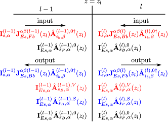
Figure 2: [Color online] Different terms occurring in Eq. (19) written for the boundary between $(l-1)$-th and $l$-th layers and the signal field. The upper index $w$ in the operators $\hat{\mathbf{A}}_{m_{a},\alpha}^{(l),w}$, $m\in\{{\rm s,i}\}$, identifies volume-emitted photon pairs ($w={\rm V}$, red color), surface-emitted photon pairs ($w={\rm S}$, blue color) and linear propagation ($w=0$, black color).

Volume SPDC as well as the linear propagation are described by one input term and one output term for each field in each layer. On the other hand, surface SPDC is described only by two output terms for both the signal and idler fields at each boundary. These fields arising in surface SPDC represent a nonlinear correction to the usual Fresnel relations at the boundaries (see Bloembergen and Pershan (1962); Bloembergen et al. (1969)) valid for linear materials. The equations arising in the separation of different terms in Eq. (19) are written in the form:

$$\mathbf{I}_{E{\rm s},\alpha}^{(l-1)}\sum_{a={\rm F,B}}\hat{\mathbf{A}}_{{\rm s}_{a},\alpha}^{(l-1),0}(z_{l}) = \mathbf{I}_{E{\rm s},\alpha}^{(l)}\sum_{a={\rm F,B}}\hat{\mathbf{A}}_{{\rm s}_{a},\alpha}^{(l),0}(z_{l}),$$ (24)

$$\mathbf{I}_{E{\rm s},\alpha}^{(l-1)}\hat{\mathbf{A}}_{{\rm s}_{\rm B},\alpha}^{(l-1),{\rm V}}(z_{l})+\mathbf{I}_{{\rm s},\alpha}^{(l-1)}\sum_{b={\rm F,B}}^{\beta={\rm x,y}}\mathbf{J}_{E{\rm s},{\rm F}b}^{\alpha\beta,(l-1)}(z_{l})\hat{\mathbf{A}}_{{\rm i}_{b},\beta}^{(l-1),0\dagger}(z_{l}) = \mathbf{I}_{E{\rm s},\alpha}^{(l)}\hat{\mathbf{A}}_{{\rm s}_{\rm F},\alpha}^{(l),{\rm V}}(z_{l})+\mathbf{I}_{{\rm s},\alpha}^{(l)}\sum_{b={\rm F,B}}^{\beta={\rm x,y}}\mathbf{J}_{E{\rm s},{\rm B}b}^{\alpha\beta,(l)}(z_{l})\hat{\mathbf{A}}_{{\rm i}_{b},\beta}^{(l),0\dagger}(z_{l}),$$ (25)

$$\mathbf{I}_{E{\rm s},\alpha}^{(l-1)}\hat{\mathbf{A}}_{{\rm s}_{\rm B},\alpha}^{(l-1),{\rm S}}(z_{l})+\mathbf{I}_{{\rm s},\alpha}^{(l-1)}\sum_{b={\rm F,B}}^{\beta={\rm x,y}}\mathbf{J}_{E{\rm s},{\rm B}b}^{\alpha\beta,(l-1)}(z_{l})\hat{\mathbf{A}}_{{\rm i}_{b},\beta}^{(l-1),0\dagger}(z_{l}) = \mathbf{I}_{E{\rm s},\alpha}^{(l)}\hat{\mathbf{A}}_{{\rm s}_{\rm F},\alpha}^{(l),{\rm S}}(z_{l})+\mathbf{I}_{{\rm s},\alpha}^{(l)}\sum_{b={\rm F,B}}^{\beta={\rm x,y}}\mathbf{J}_{E{\rm s},{\rm F}b}^{\alpha\beta,(l)}(z_{l})\hat{\mathbf{A}}_{{\rm i}_{b},\beta}^{(l),0\dagger}(z_{l}).$$ (26)

If we consider only the requirement of electric-field continuity on the boundary and omit that for the magnetic field, no surface SPDC would occur. This follows from the solution for signal-field operators $\hat{a}_{{\rm s}_{a},\alpha}(z,\omega_{\rm s})$ given in Eq. (11). The functions $\Phi_{{\rm s},{\rm B}b}^{\alpha\beta,(l-1)}(z_{l},\omega_{\rm s},\omega_{\rm i})$ and $\Phi_{{\rm s},{\rm F}b}^{\alpha\beta,(l)}(z_{l},\omega_{\rm s},\omega_{\rm i})$ equal zero [see Eq. (12)] and so the matrices $\mathbf{J}_{{\rm s},{\rm B}b}^{\alpha\beta,(l-1)}$ and $\mathbf{J}_{{\rm s},{\rm F}b}^{\alpha\beta,(l)}$ equal zero. Equations (26) thus separate from the remaining two Eqs. (24) and (25) and the operators $\hat{\mathbf{A}}_{{\rm s}_{\rm B},\alpha}^{(l-1),{\rm S}}$ and $\hat{\mathbf{A}}_{{\rm s}_{\rm F},\alpha}^{(l),{\rm S}}$ describing the surface emission could be set to zero. However, the continuity of the magnetic field requires nonzero operators $\hat{\mathbf{A}}_{{\rm s}_{\rm B},\alpha}^{(l-1),{\rm S}}$ and $\hat{\mathbf{A}}_{{\rm s}_{\rm F},\alpha}^{(l),{\rm S}}$. These operators then describe the surface emission of photon pairs at the boundary.

The requirement of continuity for the magnetic field $\hat{\mathbf{H}}_{\rm s}(z,t)$ across the boundary between the $(l-1)$-th and $l$-th layers [see Eq. (LABEL:e32)] results in the system of equations of the form written in Eqs. (24—26). These equations are formally derived from those written in Eqs. (24—26) if we replace matrix $\mathbf{I}_{E{\rm s},\alpha}^{(l)}$ by matrix $\mathbf{I}_{H{\rm s}_{a},\alpha}^{(l)}$ and matrix $\mathbf{J}_{E{\rm s},ab}^{\alpha\beta,(l)}(z)$ by matrix $\mathbf{J}_{H{\rm s},ab}^{\alpha\beta,(l)}(z)$. The matrices $\mathbf{I}_{H{\rm s}_{a},\alpha}^{(l)}$ and $\mathbf{J}_{H{\rm s},ab}^{\alpha\beta,(l)}(z)$ are defined as

$$\bigl{[}\mathbf{I}_{H{\rm s}_{a},\alpha}^{(l)}\bigr{]}_{kn}\equiv i\int_{0}^{\infty}d\omega_{\rm s}\,\frac{k_{{\rm s}_{a},\alpha}^{(l)}(\omega_{\rm s})f_{{\rm s},k}^{\ast}(\omega_{\rm s})f_{{\rm s},n}(\omega_{\rm s})}{\sqrt{n_{{\rm s},\alpha}^{(l)}(\omega_{\rm s})}},$$ (27)

$$\bigl{[}\mathbf{J}_{H{\rm s},ab}^{\alpha\beta,(l)}\bigr{]}_{kn}(z)\equiv\lambda_{H{\rm s},ab,kn}^{\alpha\beta,(l)}(z)$$ (28)

and we assume the following decomposition

$$\frac{\partial\Phi_{{\rm s},ab}^{\alpha\beta,(l)*}}{\partial z}(z,\omega_{\rm s},\omega_{\rm i})=\sum_{k,n=0}^{\infty}\lambda_{H{\rm s},ab,kn}^{\alpha\beta,(l)}(z)f_{{\rm s},k}(\omega_{\rm s})f_{{\rm i},n}(\omega_{\rm i}).$$ (29)

The boundary conditions for the free signal-field operators $\hat{\mathbf{A}}_{{\rm s}_{a},\alpha}^{(l^{\prime}),0};\,a\in\{{\rm F,B}\},\alpha\in\{{\rm x,y}\}$ arising from the continuity of the electric- [Eq. (24)] and magnetic-field amplitudes and considered for both polarizations along the ${\rm x}$ and ${\rm y}$ axes (the Fresnel relations) can be written in the following compact form

$$\mathbf{L}_{\rm s}^{(l-1)}\hat{\mathbf{A}}_{\rm s}^{(l-1),0}(z_{l})=\mathbf{L}_{\rm s}^{(l)}\hat{\mathbf{A}}_{\rm s}^{(l),0}(z_{l})$$ (30)

using the interface transition matrices $\mathbf{L}_{\rm s}^{(l)}$ Yeh (1988):

$$\mathbf{L}_{\rm s}^{(l)}=\left[\begin{array}[]{cccc}\mathbf{I}_{E{\rm s,x}}^{(l)}&\mathbf{I}_{E{\rm s,x}}^{(l)}&0&0\\ 0&0&\mathbf{I}_{E{\rm s,y}}^{(l)}&\mathbf{I}_{E{\rm s,y}}^{(l)}\\ \mathbf{I}_{H{\rm s}_{\rm F},{\rm x}}^{(l)}&\mathbf{I}_{H{\rm s}_{\rm B},{\rm x}}^{(l)}&0&0\\ 0&0&\mathbf{I}_{H{\rm s}_{\rm F},{\rm y}}^{(l)}&\mathbf{I}_{H{\rm s}_{\rm B},{\rm y}}^{(l)}\end{array}\right].$$ (31)

In Eq. (30) the signal-field operators $\hat{\mathbf{A}}_{\rm s}^{(l),0}$ are defined as follows:

$$\hat{\mathbf{A}}_{\rm s}^{(l),0}(z)\equiv\left[\begin{array}[]{c}\hat{\mathbf{A}}_{{\rm s}_{\rm F},{\rm x}}^{(l),0}(z)\\ \hat{\mathbf{A}}_{{\rm s}_{\rm B},{\rm x}}^{(l),0}(z)\\ \hat{\mathbf{A}}_{{\rm s}_{\rm F},{\rm y}}^{(l),0}(z)\\ \hat{\mathbf{A}}_{{\rm s}_{\rm B},{\rm y}}^{(l),0}(z)\end{array}\right].$$ (32)

The boundary conditions for the fields arising in volume SPDC and considered for both electric- [Eq. (25)] and magnetic-field operators can be expressed in the compact form of Eq. (30):

$$\mathbf{I}_{\rm s}(z_{l})\hat{\mathbf{A}}_{\rm s}^{\rm V}(z_{l}) = -\mathbf{J}^{(l-1)}_{{\rm s}_{\rm F}}\hat{\mathbf{A}}_{\rm i}^{(l-1),0\dagger}(z_{l})+\mathbf{J}^{(l)}_{{\rm s}_{\rm B}}\hat{\mathbf{A}}_{\rm i}^{(l),0\dagger}(z_{l}),$$

where

$$\mathbf{I}_{\rm s}(z_{l})\equiv\left[\begin{array}[]{cccc}-\mathbf{I}_{E{\rm s,x}}^{(l)}&\mathbf{I}_{E{\rm s,x}}^{(l-1)}&0&0\\ 0&0&-\mathbf{I}_{E{\rm s,y}}^{(l)}&\mathbf{I}_{E{\rm s,y}}^{(l-1)}\\ -\mathbf{I}_{H{\rm s}_{\rm F},{\rm x}}^{(l)}&\mathbf{I}_{H{\rm s}_{\rm B},{\rm x}}^{(l-1)}&0&0\\ 0&0&-\mathbf{I}_{H{\rm s}_{\rm F},{\rm y}}^{(l)}&\mathbf{I}_{H{\rm s}_{\rm B},{\rm y}}^{(l-1)}\end{array}\right]$$ (34)

and

$$\hat{\mathbf{A}}_{\rm s}^{\rm V}(z_{l})\equiv\left[\begin{array}[]{l}\hat{\mathbf{A}}_{{\rm s}_{\rm F},{\rm x}}^{(l),{\rm V}}(z_{l})\\ \hat{\mathbf{A}}_{{\rm s}_{\rm B},{\rm x}}^{(l-1),{\rm V}}(z_{l})\\ \hat{\mathbf{A}}_{{\rm s}_{\rm F},{\rm y}}^{(l),{\rm V}}(z_{l})\\ \hat{\mathbf{A}}_{{\rm s}_{\rm B},{\rm y}}^{(l-1),{\rm V}}(z_{l})\end{array}\right].$$ (35)

Matrices $\mathbf{J}^{(l)}_{{\rm s}_{a}}$, $a\in\{{\rm F,B}\}$, occurring in Eq. (II) are given as

$$\mathbf{J}^{(l)}_{{\rm s}_{a}} \equiv \left[\begin{array}[]{cccc}\mathbf{I}_{\rm s,x}^{(l)}\mathbf{J}_{E{\rm s},a{\rm F}}^{{\rm xx},(l)}(z_{l})&\mathbf{I}_{\rm s,x}^{(l)}\mathbf{J}_{E{\rm s},a{\rm B}}^{{\rm xx},(l)}(z_{l})\\ \mathbf{I}_{\rm s,y}^{(l)}\mathbf{J}_{E{\rm s},a{\rm F}}^{{\rm yx},(l)}(z_{l})&\mathbf{I}_{\rm s,y}^{(l)}\mathbf{J}_{E{\rm s},a{\rm B}}^{{\rm yx},(l)}(z_{l})\\ \mathbf{I}_{\rm s,x}^{(l)}\mathbf{J}_{H{\rm s},a{\rm F}}^{{\rm xx},(l)}(z_{l})&\mathbf{I}_{\rm s,x}^{(l)}\mathbf{J}_{H{\rm s},a{\rm B}}^{{\rm xx},(l)}(z_{l})\\ \mathbf{I}_{\rm s,y}^{(l)}\mathbf{J}_{H{\rm s},a{\rm F}}^{{\rm yx},(l)}(z_{l})&\mathbf{I}_{\rm s,y}^{(l)}\mathbf{J}_{H{\rm s},a{\rm B}}^{{\rm yx},(l)}(z_{l})\end{array}\right.$$ (45)

$$\hskip 14.22636pt\left.\begin{array}[]{cccc}\mathbf{I}_{\rm s,x}^{(l)}\mathbf{J}_{E{\rm s},a{\rm F}}^{{\rm xy},(l)}(z_{l})&\mathbf{I}_{\rm s,x}^{(l)}\mathbf{J}_{E{\rm s},a{\rm B}}^{{\rm xy},(l)}(z_{l})\\ \mathbf{I}_{\rm s,y}^{(l)}\mathbf{J}_{E{\rm s},a{\rm F}}^{{\rm yy},(l)}(z_{l})&\mathbf{I}_{\rm s,y}^{(l)}\mathbf{J}_{E{\rm s},a{\rm B}}^{{\rm yy},(l)}(z_{l})\\ \mathbf{I}_{\rm s,x}^{(l)}\mathbf{J}_{H{\rm s},a{\rm F}}^{{\rm xy},(l)}(z_{l})&\mathbf{I}_{\rm s,x}^{(l)}\mathbf{J}_{H{\rm s},a{\rm B}}^{{\rm xy},(l)}(z_{l})\\ \mathbf{I}_{\rm s,y}^{(l)}\mathbf{J}_{H{\rm s},a{\rm F}}^{{\rm yy},(l)}(z_{l})&\mathbf{I}_{\rm s,y}^{(l)}\mathbf{J}_{H{\rm s},a{\rm B}}^{{\rm yy},(l)}(z_{l})\end{array}\right].$$

Similarly, the boundary conditions for surface SPDC including both electric- [Eq. (26)] and magnetic-field operators and their polarizations are obtained in the following compact form:

$$\mathbf{I}_{\rm s}(z_{l})\hat{\mathbf{A}}_{\rm s}^{\rm S}(z_{l})=-\mathbf{J}^{(l-1)}_{{\rm s}_{\rm B}}\hat{\mathbf{A}}_{\rm i}^{(l-1),0\dagger}(z_{l})+\mathbf{J}^{(l)}_{{\rm s}_{\rm F}}\hat{\mathbf{A}}_{\rm i}^{(l),0\dagger}(z_{l}).$$ (46)

Equations (30), (II) and (46) characterize the behavior of the overall signal field at the boundaries. The idler field behaves at the boundaries in the same way and the corresponding equations characterizing its behavior are derived in the same form as those for the signal field. We remind that they are obtained from Eqs. (30), (II) and (46) by formal substitution $s\leftrightarrow i$. The equations for the signal and idler fields are mutually coupled and so we have to solve them together. For this reason, we first express them in the following ’super-vector’ and ’super-matrix’ notation:

$$\mathcal{L}^{(l-1)}\hat{\mathcal{A}}^{(l-1),0}(z_{l})=\mathcal{L}^{(l)}\hat{\mathcal{A}}^{(l),0}(z_{l}),$$ (47)

$$\mathcal{I}(z_{l})\hat{\mathcal{A}}^{\rm V}(z_{l})=-\mathcal{J}_{\rm F}^{(l-1)}\hat{\mathcal{A}}^{(l-1),0}(z_{l})+\mathcal{J}_{\rm B}^{(l)}\hat{\mathcal{A}}^{(l),0}(z_{l}),$$ (48)

$$\mathcal{I}(z_{l})\hat{\mathcal{A}}^{\rm S}(z_{l})=-\mathcal{J}_{\rm B}^{(l-1)}\hat{\mathcal{A}}^{(l-1),0}(z_{l})+\mathcal{J}_{\rm F}^{(l)}\hat{\mathcal{A}}^{(l),0}(z_{l})$$ (49)

that uses the ’super-matrices’ $\mathcal{L}^{(l)}$, $\mathcal{I}$ and $\mathcal{J}_{a}$,

$$\mathcal{L}^{(l)} \equiv \mathrm{diag}\left[\mathbf{L}_{\rm s}^{(l)},\mathbf{L}_{\rm i}^{(l)}\right],$$ (50)

$$\mathcal{I}(z_{l}) \equiv \mathrm{diag}\Bigl{[}\mathbf{I}_{\rm s}(z_{l}),\mathbf{I}_{\rm i}(z_{l})\Bigr{]},$$ (51)

$$\mathcal{J}_{a}^{(l)} \equiv \mathrm{adiag}\left[\mathbf{J}_{{\rm s}_{a}}^{(l)},\mathbf{J}_{{\rm i}_{a}}^{(l)}\right];\,a\in\{{\rm F,B}\}.$$ (52)

Symbol ${\rm diag}$ (${\rm adiag}$) stands for a diagonal (anti-diagonal) matrix. ’Super-vector’ operators $\hat{\mathcal{A}}^{(l),0}(z)$, $\hat{\mathcal{A}}^{\rm V}(z_{l})$ and $\hat{\mathcal{A}}^{\rm S}(z_{l})$ introduced in Eqs. (50—52) are defined as

$$\hat{\mathcal{A}}^{(l),0}(z) =\left[\begin{array}[]{c}\hat{\mathbf{A}}^{(l)}_{\rm s}(z)\\ \hat{\mathbf{A}}^{(l)\dagger}_{\rm i}(z)\end{array}\right],$$ (55)

$$\hat{\mathcal{A}}^{w}(z_{l}) =\left[\begin{array}[]{c}\hat{\mathbf{A}}^{w}_{\rm s}(z_{l})\\ \hat{\mathbf{A}}^{w\dagger}_{\rm i}(z_{l})\end{array}\right];\hskip 14.22636ptw\in\{{\rm S,V}\}.$$ (58)

The free-field operators $\hat{\mathcal{A}}^{(l),0}$, $l\in\{1,\ldots,N\}$, represent the source of photon-pairs emitted either in the volume of layers [Eq. (48)] or at the boundaries between the layers [Eq. (49)]. To quantify both volume and surface SPDC, we need to express these operators in terms of those impinging on the crystal. We first derive the relations between operators $\hat{\mathcal{A}}^{(l),0}$ at the left and right boundaries of an $l$-th homogeneous layer. Using Eqs. (13), (17) and (18) we arrive at the formula

$$\hat{\mathbf{A}}_{\rm s}^{(l),0}(z_{l+1})=\mathbf{P}_{\rm s}^{(l)}\hat{\mathbf{A}}_{\rm s}^{(l),0}(z_{l})$$ (59)

in which the matrix $\mathbf{P}_{\rm s}^{(l)}$ is given as

$$\mathbf{P}_{\rm s}^{(l)}\equiv\mathrm{diag}\left[\mathbf{P}_{{\rm s}_{\rm F},{\rm x}}^{(l)},\mathbf{P}_{{\rm s}_{\rm B},{\rm x}}^{(l)},\mathbf{P}_{{\rm s}_{\rm F},{\rm y}}^{(l)},\mathbf{P}_{{\rm s}_{\rm B},{\rm y}}^{(l)}\right],$$ (60)

and

$$\bigl{[}\mathbf{P}_{{\rm s}_{a},\alpha}^{(l)}\bigr{]}_{kn}=\int_{0}^{\infty}d\omega_{\rm s}\,\exp[ik_{{\rm s}_{a},\alpha}^{(l)}(\omega_{\rm s})L_{l}]f_{{\rm s},k}^{*}(\omega_{\rm s})f_{{\rm s},n}(\omega_{\rm s}).$$

For ’super-vector’ $\hat{\mathcal{A}}^{(l),0}$ containing both signal- and idler-field operators, Eq. (59) attains the form

$$\hat{\mathcal{A}}^{(l),0}(z_{l+1})=\mathcal{P}^{(l)}\hat{\mathcal{A}}^{(l),0}(z_{l})$$ (62)

and

$$\mathcal{P}^{(l)}=\left[\begin{array}[]{cc}\mathbf{P}_{\rm s}^{(l)}&0\\ 0&\mathbf{P}_{\rm i}^{(l)}\end{array}\right].$$ (63)

The operators $\hat{\mathcal{A}}^{(0),0}(z_{1})$ at the left-hand side of the structure and operators $\hat{\mathcal{A}}^{(N+1),0}(z_{N+1})$ at the right-hand side of the structure are related by the following equation

$$\hat{\mathcal{A}}^{(N+1),0}(z_{N+1})=\mathcal{T}^{(N+1,0)}\hat{\mathcal{A}}^{(0),0}(z_{1})$$ (64)

where

$$\mathcal{T}^{(n,m)} \equiv \mathcal{D}^{(n)-1}\left(\prod_{l={m+1}^{n}-1}\mathcal{D}^{(l)}\mathcal{P}^{(l)}\mathcal{D}^{(l)-1}\right)\mathcal{D}^{(m)};$$ (65)

$$\hskip 14.22636ptm,n\in\{0,\ldots,N+1\},n>m.$$

In Eq. (65), terms in the product are multiplied from the right to the left as index $l$ increases. If $n=m+1$, the product in Eq. (65) is set to unity by definition. The general transfer matrix $\mathcal{T}^{(n,m)}$ defined in Eq. (65) transfers the operators from the right boundary of layer $m$ ($z=z_{m}$) to the left boundary of layer $n$ ($z=z_{n-1}$) (see Fig. 1). The matrix $\mathcal{T}^{(N+1,0)}$ then describes the propagation through the whole layered structure.

The operators $\hat{\mathbf{A}}_{a,\alpha}^{(N+1),0}(z_{N+1})$ and $\hat{\mathbf{A}}_{a,\alpha}^{(0),0}(z_{1})$ embedded in the ’super-vectors’ $\hat{\mathcal{A}}^{(N+1),0}(z_{N+1})$ and $\hat{\mathcal{A}}^{(0),0}(z_{1})$, respectively, have to be rearranged to express the field operators leaving the structure [$\hat{\mathbf{A}}_{{\rm F},\alpha}^{(N+1),0}(z_{N+1})$ and $\hat{\mathbf{A}}_{{\rm B},\alpha}^{(0),0}(z_{1})$] in terms of the operators entering the structure [$\hat{\mathbf{A}}_{{\rm F},\alpha}^{(0),0}(z_{1})$ and $\hat{\mathbf{A}}_{{\rm B},\alpha}^{(N+1),0}(z_{N+1})$]. As the relations among the considered field operators are linear, the needed formulas are easily found. To express them, we introduce the notation in which the signal- and idler-field operators are suitably rearranged:

$$\hat{\mathcal{A}}^{{\rm(out)},w}=\left[\begin{array}[]{l}\hat{\mathbf{A}}_{\rm F,x}^{(N+1),w}\\ \hat{\mathbf{A}}_{\rm B,x}^{(0),w}\\ \hat{\mathbf{A}}_{\rm F,y}^{(N+1),w}\\ \hat{\mathbf{A}}_{\rm B,y}^{(0),w}\end{array}\right],\,\hat{\mathcal{A}}^{{\rm(in)},w}=\left[\begin{array}[]{l}\hat{\mathbf{A}}_{\rm F,x}^{(0),w}\\ \hat{\mathbf{A}}_{\rm B,x}^{(N+1),w}\\ \hat{\mathbf{A}}_{\rm F,y}^{(0),w}\\ \hat{\mathbf{A}}_{\rm B,y}^{(N+1),w}\end{array}\right]$$ (66)

and

$$\hat{\mathbf{A}}_{a,\alpha}^{(l),w}(z) \equiv \left[\begin{array}[]{c}\hat{\mathbf{A}}_{{\rm s}_{a},\alpha}^{(l),w}(z)\\ \hat{\mathbf{A}}_{{\rm i}_{a},\alpha}^{(l),w\dagger}(z)\end{array}\right],\hskip 14.22636ptw\in\{0,{\rm S,V}\},$$ (69)

$$\hskip 14.22636pt\,a\in\{{\rm F,B}\},\alpha\in\{{\rm x,y}\}.$$

In this notation, the input-output formulas for the fields’ operators are written as

$$\hat{\mathcal{A}}^{\rm(out),0}=\mathcal{F}\,\hat{\mathcal{A}}^{\rm(in),0}.$$ (70)

Detailed calculations reveal the matrix $\mathcal{F}$ in the form:

$$\mathcal{F} \equiv \mathcal{U}^{-1}\mathcal{V},$$ (81)

$$\mathcal{U}\equiv\left[\begin{array}[]{rrrr}1&-[\mathcal{T}]_{\rm Fx,Bx}&0&-[\mathcal{T}]_{\rm Fx,By}\\ 0&-[\mathcal{T}]_{\rm Bx,Bx}&0&-[\mathcal{T}]_{\rm Bx,By}\\ 0&-[\mathcal{T}]_{\rm Fy,Bx}&1&-[\mathcal{T}]_{\rm Fy,By}\\ 0&-[\mathcal{T}]_{\rm By,Bx}&0&-[\mathcal{T}]_{\rm By,By}\end{array}\right],$$

$$\mathcal{V}\equiv\left[\begin{array}[]{rrrr}[\mathcal{T}]_{\rm Fx,Fx}&0&[\mathcal{T}]_{\rm Fx,Fy}&0\\ \left[\mathcal{T}\right]_{\rm Bx,Fx}&-1&[\mathcal{T}]_{\rm Bx,Fy}&0\\ \left[\mathcal{T}\right]_{\rm Fy,Fx}&0&[\mathcal{T}]_{\rm Fy,Fy}&0\\ \left[\mathcal{T}\right]_{\rm By,Fx}&0&[\mathcal{T}]_{\rm By,Fy}&-1\end{array}\right].$$

We remind that the operators $\hat{\mathbf{A}}_{a,\alpha}^{(N+1),0}$ at the right-hand side of the structure are evaluated at position $z_{N+1}$, whereas the operators $\hat{\mathbf{A}}_{a,\alpha}^{(0),0}$ at the left-hand side of the structure are determined at position $z_{1}$. In the definitions of matrices $\mathcal{U}$ and $\mathcal{V}$ in Eq. (81), symbol $1$ means the diagonal unity matrix of appropriate dimensions.

Utilizing transformations (64) and (70) the operators $\mathcal{\hat{A}}^{(l),0}(z_{l})$ in layer $l$ are expressed in terms of the input operators as

$$\hat{\mathcal{A}}^{(l),0}(z_{l})=\mathcal{T}^{(l,0)}\mathcal{W}\,\hat{\mathcal{A}}^{\rm(in),0}$$ (82)

using matrix $\mathcal{W}$ defined as

$$\mathcal{W}\equiv\left[\begin{array}[]{cccc}1&0&0&0\\ \left[\mathcal{F}\right]{}_{\rm Bx,Fx}&\left[\mathcal{F}\right]{}_{\rm Bx,Bx}&\left[\mathcal{F}\right]{}_{\rm Bx,Fy}&\left[\mathcal{F}\right]{}_{\rm Bx,By}\\ 0&0&1&0\\ \left[\mathcal{F}\right]_{\rm By,Fx}&\left[\mathcal{F}\right]_{\rm By,Bx}&\left[\mathcal{F}\right]_{\rm By,Fy}&\left[\mathcal{F}\right]_{\rm By,By}\end{array}\right].$$ (83)

Exploiting Eqs. (59) and (82) the operators $\mathcal{\hat{A}}^{(l),0}(z_{l+1})$ are expressed via the input operators along the relation:

$$\mathcal{\hat{A}}^{(l),0}(z_{l+1})=\mathcal{P}^{(l)}\mathcal{T}^{(l,0)}\mathcal{W}\,\hat{\mathcal{A}}^{\rm(in),0}.$$ (84)

The operators $\hat{\mathcal{A}}^{\rm V}(z_{l})$ and $\hat{\mathcal{A}}^{\rm S}(z_{l})$ determined in Eqs. (48) and (49), respectively, describe photons born in volume and surface SPDC. Such photons, after being emitted in a given layer or at a given boundary, propagate as free fields towards the output planes of the structure. This propagation obeys the following linear relations:

$$\hat{\mathcal{A}}^{w}(z_{l})=\mathcal{X}(z_{l})\mathcal{Y}\,\hat{\mathcal{A}}^{{\rm(out)},w};\,w\in\{{\rm S,V}\}.$$ (85)

In Eq. (85), matrices $\mathcal{X}(z_{l})$ and $\mathcal{Y}$ are defined along the relations:

$$\mathcal{X}(z_{l}) \equiv \left[\begin{array}[]{cc}\left[\mathcal{T}^{(l,0)}\right]_{\rm Fx,Fx}&\left[\mathcal{T}^{(l,0)}\right]_{\rm Fx,Bx}\\ \left[\tilde{\mathcal{T}}^{(l,0)}\right]_{\rm Bx,Fx}&\left[\tilde{\mathcal{T}}^{(l,0)}\right]_{\rm Bx,Bx}\\ \left[\mathcal{T}^{(l,0)}\right]_{\rm Fy,Fx}&\left[\mathcal{T}^{(l,0)}\right]_{\rm Fy,Bx}\\ \left[\tilde{\mathcal{T}}^{(l,0)}\right]_{\rm By,Fx}&\left[\tilde{\mathcal{T}}^{(l,0)}\right]_{\rm By,Bx}\end{array}\right.$$ (95)

$$\hskip 14.22636pt\left.\begin{array}[]{cc}\left[\mathcal{T}^{(l,0)}\right]_{\rm Fx,Fy}&\left[\mathcal{T}^{(l,0)}\right]_{\rm Fx,By}\\ \left[\tilde{\mathcal{T}}^{(l,0)}\right]_{\rm Bx,Fy}&\left[\tilde{\mathcal{T}}^{(l,0)}\right]_{\rm Bx,By}\\ \left[\mathcal{T}^{(l,0)}\right]_{\rm Fy,Fy}&\left[\mathcal{T}^{(l,0)}\right]_{\rm Fy,By}\\ \left[\tilde{\mathcal{T}}^{(l,0)}\right]_{\rm By,Fy}&\left[\tilde{\mathcal{T}}^{(l,0)}\right]_{\rm By,By}\end{array}\right],$$

$$\mathcal{Y} \equiv \left[\begin{array}[]{cccc}\left[\mathcal{Z}\right]_{\rm Fx,Fx}&\left[\mathcal{Z}\right]_{\rm Fx,Bx}&\left[\mathcal{Z}\right]_{\rm Fx,Fy}&\left[\mathcal{Z}\right]_{\rm Fx,By}\\ 0&1&0&0\\ \left[\mathcal{Z}\right]_{\rm Fy,Fx}&\left[\mathcal{Z}\right]_{\rm Fy,Bx}&\left[\mathcal{Z}\right]_{\rm Fy,Fy}&\left[\mathcal{Z}\right]_{\rm Fy,By}\\ 0&0&0&1\end{array}\right].$$ (100)

In Eq. (95), $\tilde{\mathcal{T}}^{(l,0)}=\mathcal{P}^{(l)}\mathcal{T}^{(l,0)}$. The matrix $\mathcal{Z}$ occurring in Eq. (100) stands for the inverse matrix to $\mathcal{F}$ defined in Eq. (81).

Now we return back to the central equations (48) and (49) that describe the emission of photon pairs around the boundary surrounded by the $(l-1)$-th and $l$-th layers. Whereas Eq. (48) describes photons emitted in volume SPDC and propagating forward in the $(l-1)$-th layer and backward in the $l$-th layer, Eq. (49) characterizes photon pairs coming from surface SPDC occurring at the boundary between the two layers. The ’local’ operators occurring in these equations have to be replaced by those describing the fields outside the structure and mutually related by free-field propagation. The operators of the fields impinging on the boundary from the left- as well as right-hand side are replaced by those entering the structure applying Eq. (82). On the other hand, the operators characterizing the fields propagating out of the boundary are substituted by those appropriate for the fields leaving the whole structure with the help of Eq. (85). This results in the relation between the input and output operators of the fields describing one photon pair born around the boundary of the $(l-1)$-th and $l$-th layers:

$$\hat{\mathcal{A}}^{{\rm(out)},w}_{(l)}=\mathcal{S}^{(l,l-1),w}\hat{\mathcal{A}}^{\rm(in),0};\hskip 8.53581ptw\in\{{\rm S,V}\}$$ (102)

and

$$\mathcal{S}^{(l,l-1),{\rm V}} = \left[\mathcal{I}(z_{l})\mathcal{X}(z_{l})\mathcal{Y}\right]^{-1}$$

$$\left(-\mathcal{J}_{\rm F}^{(l-1)}\tilde{\mathcal{T}}^{(l-1,0)}+\mathcal{J}_{\rm B}^{(l)}\mathcal{T}^{(l,0)}\right)\mathcal{W},$$

$$\mathcal{S}^{(l,l-1),{\rm S}} = \left[\mathcal{I}(z_{l})\mathcal{X}(z_{l})\mathcal{Y}\right]^{-1}$$ (103)

$$\left(-\mathcal{J}_{\rm B}^{(l-1)}\tilde{\mathcal{T}}^{(l-1,0)}+\mathcal{J}_{\rm F}^{(l)}\mathcal{T}^{(l,0)}\right)\mathcal{W}.$$

The overall operators of the fields at the output of the structure are given by coherent superposition of the contributions from all layers and their boundaries:

$$\hat{\mathcal{A}}^{{\rm(out)},w} = \mathcal{G}^{w}\,\hat{\mathcal{A}}^{\rm(in),0},$$

$$\mathcal{G}^{w} = \sum_{l=1}^{N+1}\mathcal{S}^{(l,l-1),w};\,w\in\{{\rm S,V}\}.$$ (104)

Knowing relation (II) between the operators $\hat{\mathcal{A}}^{{\rm(out)},w}$, $w\in\{{\rm S,V}\}$, and $\hat{\mathcal{A}}^{\rm(in),0}$, the application of transformations given in Eqs. (17) and (18) provides the formula expressing the output signal-field operators $\hat{a}_{{\rm s}_{a},\alpha}^{\rm(out)}$ in terms of the input idler-field operators $\hat{\bar{a}}_{{\rm i}_{b},\beta}^{{\rm(in)}\dagger}$:

$$\hat{a}_{{\rm s}_{a},\alpha}^{{\rm(out)},w}(\omega_{\rm s}) = \mathbf{f}_{\rm s}^{\rm T}(\omega_{\rm s})\sum_{b={\rm F,B}}^{\beta={\rm x,y}}\bigl{[}\mathcal{G}^{w}\bigr{]}_{{\rm s}_{a}\alpha,{\rm i}_{b}\beta}\int_{0}^{\infty}d\omega_{\rm i}\mathbf{f}_{\rm i}(\omega_{\rm i})$$ (105)

$$\times\hat{\bar{a}}_{{\rm i}_{b},\beta}^{{\rm(in)},0\dagger}(\omega_{\rm i});\hskip 8.53581ptw\in\{{\rm S,V}\},$$

$$\,a\in\{{\rm F,B}\},\alpha\in\{{\rm x,y}\}.$$

The output signal-field operators $\hat{a}_{{\rm s}_{\rm F},\alpha}^{{\rm(out)},w}\equiv\hat{a}_{{\rm s}_{\rm F},\alpha}^{(N+1),w}(z_{N+1},\omega_{\rm s})$ [$\hat{a}_{{\rm s}_{\rm B},\alpha}^{{\rm(out)},w}\equiv\hat{a}_{{\rm s}_{\rm B},\alpha}^{(0),w}(z_{1},\omega_{\rm s})$] are located at the position $z=z_{N+1}$ [$z=z_{1}$]. On the other hand, the input idler-field operators $\hat{\bar{a}}_{{\rm i}_{\rm F},\beta}^{\rm(in),0}\equiv\hat{\bar{a}}_{{\rm i}_{\rm F},\beta}^{\rm(0)}(z_{1},\omega_{\rm i})$ [$\hat{\bar{a}}_{{\rm i}_{\rm B},\beta}^{\rm(in),0}\equiv\hat{\bar{a}}_{{\rm i}_{\rm B},\beta}^{\rm(N+1)}(z_{N+1},\omega_{\rm i})$] characterize the field at position $z_{1}$ [$z_{N+1}$]. In Eq. (105), vectors $[\mathbf{f}_{m}](\omega_{m})$ containing elements $f_{m,k}(\omega_{m})$ for $m\in\{{\rm s,i}\}$ have been introduced, symbol $\bigl{[}\mathcal{G}^{w}\bigr{]}_{{\rm s}_{a}\alpha,{\rm i}_{b}\beta}$ denotes a sub-matrix of matrix $\mathcal{G}^{w}$ identified by its indices and symbol ${\rm T}$ stands for transposition.

In parallel with Eq. (105), the formula for linear propagation of the signal-field operators $\hat{\bar{a}}_{{\rm s}_{a},\alpha}^{0}$ from the input of the layered structure to its output including scattering of the field at the boundaries is determined from Eq. (70):

$$\hat{\bar{a}}_{{\rm s}_{a},\alpha}^{\rm(out),0}(\omega_{\rm s}) \equiv \mathbf{f}_{\rm s}^{\rm T}(\omega_{\rm s})\sum_{b={\rm F,B}}^{\beta={\rm x,y}}\bigl{[}\mathcal{F}\bigr{]}_{{\rm s}_{a}\alpha,{\rm s}_{b}\beta}\int_{0}^{\infty}d\omega_{\rm s}^{\prime}\mathbf{f}_{\rm s}^{*}(\omega_{\rm s}^{\prime})$$ (106)

$$\times\hat{\bar{a}}_{{\rm s}_{b},\beta}^{\rm(in),0}(\omega_{\rm s}^{\prime});\hskip 8.53581pta\in\{{\rm F,B}\},\alpha\in\{{\rm x,y}\}.$$

III Experimental characteristics of photon pairs

The emitted photon pairs are characterized by the joint signal-idler photon-number density $n_{ab}^{\alpha\beta}$ defined along the relation:

$$n_{ab}^{\alpha\beta}(\omega_{\rm s},\omega_{\rm i}) = \langle\mathrm{vac}|\hat{a}_{{\rm s}_{a},\alpha}^{{\rm(out)}\dagger}(\omega_{\rm s})\hat{a}_{{\rm s}_{a},\alpha}^{\rm(out)}(\omega_{\rm s})$$ (107)

$$\times\hat{a}_{{\rm i}_{b},\beta}^{{\rm(out)}\dagger}(\omega_{\rm i})\hat{a}_{{\rm i}_{b},\beta}^{\rm(out)}(\omega_{\rm i})|\mathrm{vac}\rangle.$$

The photon-number density $n_{ab}^{\alpha\beta}(\omega_{\rm s},\omega_{\rm i})$ gives the density of photon pairs with a signal photon at frequency $\omega_{\rm s}$ propagating in direction $a$ with polarization $\alpha$ and its idler twin at frequency $\omega_{\rm i}$ propagating in direction $b$ with polarization $\beta$. Assuming vacuum around the structure and using Eqs. (105) and (106), we arrive at the formula:

$$n_{ab}^{\alpha\beta}(\omega_{\rm s},\omega_{\rm i}) = \sum_{w,w^{\prime}={\rm S,V}}\sum_{g={\rm F,B}}^{\gamma={\rm x,y}}\mathbf{f}_{\rm i}^{*,{\rm T}}(\omega_{\rm i})\bigl{[}\mathcal{F}\bigr{]}_{{\rm i}_{b}\beta,{\rm i}_{g}\gamma}$$ (108)

$$\times\bigl{[}\mathcal{G}^{w}\bigr{]}_{{\rm s}_{a}\alpha,{\rm i}_{g}\gamma}^{\rm T}\mathbf{f}_{\rm s}^{*}(\omega_{\rm s})\sum_{d={\rm F,B}}^{\delta={\rm x,y}}\mathbf{f}_{\rm s}^{\rm T}(\omega_{\rm s})\bigl{[}\mathcal{F}\bigr{]}_{{\rm s}_{a}\alpha,{\rm s}_{d}\delta}$$

$$\times\bigl{[}\mathcal{G}^{w^{\prime}}\bigr{]}_{{\rm i}_{b}\beta,{\rm s}_{d}\delta}^{*,\rm T}\mathbf{f}_{\rm i}(\omega_{\rm i})+{\rm h.c.}$$

$$\equiv n_{ab}^{\alpha\beta,{\rm V}}(\omega_{\rm s},\omega_{\rm i})+n_{ab}^{\alpha\beta,{\rm S}}(\omega_{\rm s},\omega_{\rm i})$$

$$+n_{ab}^{\alpha\beta,{\rm I}}(\omega_{\rm s},\omega_{\rm i})$$

$$\equiv n_{ab}^{\alpha\beta,{\rm SV}}.$$

According to Eq. (108), the joint photon-number density $n_{ab}^{\alpha\beta}$ is decomposed into three contributions: The first contribution $n_{ab}^{\alpha\beta,{\rm V}}$ originates in volume SPDC [$w=w^{\prime}={\rm V}$ in the sum at the first line of Eq. (108)], the second contribution $n_{ab}^{\alpha\beta,{\rm S}}$ arises in surface SPDC ($w=w^{\prime}={\rm S}$) and the last contribution $n_{ab}^{\alpha\beta,{\rm I}}$ occurs due to interference between the volume and surface contributions. However, these contributions cannot be mutually separated in the considered 1D model in the experiment. That is why the three contributions summed together give the overall joint photon-number density $n_{ab}^{\alpha\beta,{\rm SV}}$.

The signal photon-number density $n_{s,ab}^{\alpha\beta,w}$ defined for $w\in\{{\rm S,V,SV}\}$ is derived along the relation

$$n_{{\rm s},ab}^{\alpha\beta,w}(\omega_{\rm s})=\int_{0}^{\infty}d\omega_{\rm i}\,n_{ab}^{\alpha\beta,w}(\omega_{\rm s},\omega_{\rm i}).$$ (109)

Similarly, the number $N_{ab}^{\alpha\beta,w}$ of emitted photon pairs is given by the formula

$$N_{ab}^{\alpha\beta,w}=\int_{0}^{\infty}d\omega_{\rm s}\,n_{{\rm s},ab}^{\alpha\beta,w}(\omega_{\rm s}).$$ (110)

The ratio $\eta_{{\rm s},ab}^{\alpha\beta}$ of signal photon-number density $n_{{\rm s},ab}^{\alpha\beta,{\rm S}}$ emitted by surface SPDC and density $n_{{\rm s},ab}^{\alpha\beta,{\rm V}}$ arising in volume SPDC,

$$\eta_{{\rm s},ab}^{\alpha\beta}(\omega_{\rm s})\equiv\frac{n_{{\rm s},ab}^{\alpha\beta,S}(\omega_{\rm s})}{n_{{\rm s},ab}^{\alpha\beta,{\rm V}}(\omega_{\rm s})},$$ (111)

provides insight into the nature of the whole SPDC process. For the photon numbers, we define the ratio $R_{ab}^{\alpha\beta}$ of number $N_{ab}^{\alpha\beta,{\rm S}}$ of photon pairs emitted at the boundaries and number $N_{ab}^{\alpha\beta,{\rm V}}$ of photon pairs created inside the layers:

$$R_{ab}^{\alpha\beta}\equiv\frac{N_{ab}^{\alpha\beta,{\rm S}}}{N_{ab}^{\alpha\beta,{\rm V}}}.$$ (112)

To reveal temporal characteristics of photon pairs, we define the following spectral amplitude correlation function, that plays the role of the usual spectral two-photon amplitude:

$$\phi_{ab}^{\alpha\beta}(\omega_{\rm s},\omega_{\rm i})=\langle\mathrm{vac}|\hat{a}_{{\rm s}_{a},\alpha}^{(\rm out)}(\omega_{\rm s})\hat{a}_{{\rm i}_{b},\beta}^{(\rm out)}(\omega_{\rm i})|\mathrm{vac}\rangle.$$ (113)

Its Fourier transform provides us a temporal two-photon amplitude $\tilde{\phi}_{ab}^{\alpha\beta}(t_{\rm s},t_{\rm i})$ that gives the probability amplitude of detecting a signal photon propagating in direction $a$ and polarized in direction $\alpha$ at time $t_{\rm s}$ together with its idler twin propagating in direction $b$ with polarization $\beta$ at time $t_{\rm i}$:

$$\tilde{\phi}_{ab}^{\alpha\beta}(t_{\rm s},t_{\rm i}) = \int_{0}^{\infty}d\omega_{\rm s}\int_{0}^{\infty}d\omega_{\rm i}\,\phi_{ab}^{\alpha\beta}(\omega_{\rm s},\omega_{\rm i})$$ (114)

$$\mbox{}\times\exp(-i\omega_{\rm s}t_{\rm s}-i\omega_{\rm i}t_{\rm i}).$$

The corresponding normalized probability density $p_{ab}^{\alpha\beta}$ is then obtained by the formula

$$p_{ab}^{\alpha\beta}(t_{\rm s},t_{\rm i})=\frac{|\phi_{ab}^{\alpha\beta}(t_{\rm s},t_{\rm i})|^{2}}{\int_{-\infty}^{\infty}dt_{\rm s}^{\prime}\int_{-\infty}^{\infty}dt_{\rm i}^{\prime}|\phi_{ab}^{\alpha\beta}(t_{\rm s}^{\prime},t_{\rm i}^{\prime})|^{2}}.$$ (115)

The temporal two-photon amplitude $\tilde{\phi}_{ab}^{\alpha\beta}$ also allows us to determine the normalized signal-field photon flux $p_{{\rm s},ab}^{\alpha\beta}$:

$$p_{{\rm s},ab}^{\alpha\beta}(t_{\rm s})=\int_{-\infty}^{\infty}dt_{\rm i}\,p_{ab}^{\alpha\beta}(t_{\rm s},t_{\rm i}).$$ (116)

IV Properties of the emitted photon pairs

In this section, we consider a typical nonlinear layered structure made of alternating GaN/AlN layers under usual experimental conditions. We assume a pump beam at central wavelength $\lambda_{\rm p}^{0}=400$ nm that impinges on the structure at normal incidence from its left, is polarized along the ${\rm y}$ axis and has a Gaussian spectral profile:

$$A_{{\rm p}_{\rm F},{\rm y}}^{(0)}(\omega_{\rm p})=\sqrt{\sqrt{\frac{\mu_{0}}{\varepsilon_{0}\pi}}\frac{E}{\pi\sigma_{\rm p}}}\exp\left[-\frac{(\omega_{\rm p}-\omega_{\rm p}^{0})^{2}}{2\sigma_{\rm p}^{2}}\right].$$ (117)

The remaining input amplitudes $A_{{\rm p}_{\rm B},{\rm y}}^{(N+1)}(\omega_{\rm p})$, $A_{{\rm p}_{\rm F},{\rm x}}^{(0)}(\omega_{\rm p})$ and $A_{{\rm p}_{\rm B},{\rm x}}^{(N+1)}(\omega_{\rm p})$ of the pump field are assumed to be zero. In the analysis, the pump-beam energy $E$ per unit area equals $1\times 10^{3}$ J/m² ($1$ mJ/mm²) per one pulse. The pump-beam spectral width $\sigma_{\rm p}$ is set such that the pump-beam intensity spectral width (FWHM, full width in the half of maximum) equals 7 nm. Assuming a transformed limited pump pulse, its intensity temporal width equals 33 fs (FWHM). In the analysis, we focus on the properties of photon pairs with both photons propagating forward and the signal photon polarized along the ${\rm x}$-axis together with its idler twin polarized along the ${\rm y}$-axis. For simplicity, we omit both propagation and polarization indices in the following discussion.

To obtain an efficient nonlinear layered structure, all three interacting fields have to be sufficiently enhanced by back-scattering inside the structure. This requires localization of the fields into transmission peaks found near band gaps (for details, Peřina Jr. (2011)). This can be accomplished in two steps. In the first step, layered structures with the pump beam localized in a transmission peak near the band gap are identified. Then, in the second step, the identified structures are analyzed and those exhibiting the largest number of emitted photon pairs are chosen.

The considered structures were composed of 10 GaN and 10 AlN mutually alternating layers. Their lengths $l_{1}$ (GaN) and $l_{2}$ (AlN) were assumed in interval $(10\text{~{}nm},100\text{~{}nm})$, in which the greatest enhancement of fields’ amplitudes occurs. The linear intensity transmission coefficient $T_{p}$ for the pump beam at central wavelength $\lambda_{\rm p}^{0}$ and for the considered GaN/AlN structures is plotted in Fig. 3. It exhibits periodically alternating transmission and reflection bands. In Fig. 3, the band gaps are found in blue regions whereas the transmission peaks are indicated by red curves. Four transmission peaks indicated by black curves in Fig. 3 are highlighted ($L_{j}$, $j=1,\ldots,4$). The peaks denoted as $L_{2}$ and $L_{3}$ occur next to a band gap and so, according to the theory of band-gap structures, they provide the greatest enhancement of pump-field amplitudes. For comparison, we also analyze the structures lying in peaks $L_{1}$ and $L_{4}$.

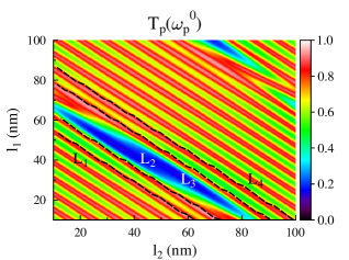
Figure 3: [Color online] Topo graph of linear intensity transmission coefficient $T_{p}$ as it depends on layers’ lengths $l_{1}$ and $l_{2}$ for the pump beam at wavelength $\lambda_{\rm p}^{0}=400$ nm and structure having 10 double layers GaN/AlN. Black dashed curves denoted as $L_{1}$, $L_{2}$, $L_{3}$, and $L_{4}$ indicate transmission peaks of the structures used in further analysis.

The overall number $N^{\rm SV}$ of emitted photon pairs for the structures lying on curves $L_{1}$, $L_{2}$, $L_{3}$, and $L_{4}$ defined in the graph of Fig. 3 is determined in the second step to find the most efficient structures. For all four curves, the number $N^{\rm SV}$ of emitted photon pairs increases with the increasing length $l_{1}$ of nonlinear GaN layers (see the curves in Fig. 4). This increase originates in the increasing amount of nonlinear GaN material inside the structure. However, the observed dependence is nontrivial as interference of the fields back-scattered inside the structure depends strongly on the layers’ lengths $l_{1}$ and $l_{2}$. The number $N^{\rm SV}$ of emitted photon pairs increases faster for the structures lying on curves $L_{1}$ and $L_{2}$ situated below the band gap compared to those found at curves $L_{3}$ and $L_{4}$ positioned above the band gap. This is probably caused by the fact that the pump-field amplitudes along the structure are localized preferably in the nonlinear GaN layers for the peaks below the band gap, contrary to the peaks above the band gap in which the pump-field amplitudes are preferably localized in the linear AlN layers.

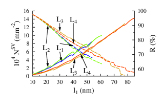
Figure 4: [Color online] Number $N^{\rm SV}$ of photon pairs emitted in both volume and surface SPDC (full curves) and ratio $R$ of photon-pair number arising in surface SPDC and that coming from volume SPDC (dashed curves) as they depend on GaN layers’ length $l_{1}$. The quantities are drawn for curves $L_{1}$ (blue curves), $L_{2}$ (green), $L_{3}$ (yellow) and $L_{4}$ (red) defined in Fig. 3.

Contrary to the overall number $N^{\rm SV}$ of emitted photon pairs, the ratio $R$ of photon-pair number $N^{\rm S}$ emitted at the surfaces and number $N^{\rm V}$ of photon pairs created in the volume decreases with the increasing length $l_{1}$ of GaN layers. This is so as the number $N^{\rm S}$ of photon pairs emitted at surfaces decreases with the increasing length $l_{1}$ and, simultaneously, the number $N^{\rm V}$ of photon pairs generated in the volume raises as the length $l_{1}$ increases. Decrease in the ratio $R$ is faster for curves $L_{1}$ and $L_{2}$ as the number $N^{\rm V}$ of photon pairs plotted as a function of length $l_{1}$ raises faster.

For detailed analysis, we have chosen a structure composed of 10 GaN layers $l_{1}=60$ nm long and 10 AlN layers $l_{2}=13$ nm long. Its joint signal-idler spectral photon-number density $n^{\rm SV}$ for the whole SPDC process is drawn in Fig. 5(a). Photon-pair emission occurs in the broad frequency range. Three main peaks can be found in the spectral density $n^{\rm SV}$ of both signal and idler fields shown in Fig. 5(b). The main peaks are found at the central frequencies $2\omega_{\rm s}/\omega_{\rm p}^{0}=2\omega_{\rm i}/\omega_{\rm p}^{0}=1$ where $n^{\rm SV}=4.97\times 10^{-33}$. On the other hand, the profile of photon-number density $n^{\rm SV}$ plotted as a function of the difference $\omega_{\rm s}-\omega_{\rm i}$ of the signal and idler frequencies is narrow as its spread is dominantly given by the pump-field spectral width.

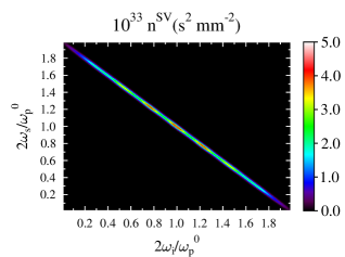
(a)

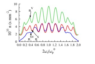
(b)

Figure 5: [Color online] (a) Joint signal-idler spectral photon-number density $n^{\rm SV}$ of complete SPDC and (b) profiles of joint signal-idler spectral photon-number densities $n^{\rm S}$ (red curve), $n^{\rm V}$ (green) and $n^{\rm SV}$ (blue) arising in turn in surface, volume and complete SPDC along the line $\omega_{\rm s}+\omega_{\rm i}=\omega_{\rm p}^{0}$ as they depend on normalized signal frequency $\omega_{\rm s}/\omega_{\rm p}^{0}$; $N=20$, $l_{1}=60$ nm, $l_{2}=13$ nm, $\lambda_{\rm p}^{0}=400$ nm.

To get insight into the origin of photon pairs generated in SPDC, we compare in parallel the contribution of volume SPDC and surface SPCD to the complete SPDC process. These contributions are compared in Fig. 5(b) where the profiles of the corresponding joint signal-idler spectral photon-number densities $n$ taken along the line $\omega_{\rm s}+\omega_{\rm i}=\omega_{\rm p}^{0}$ are plotted. There occur nine resonant peaks in the profiles $n^{\rm S}$ and $n^{\rm V}$ belonging to volume and surface SPDC, respectively. Contrary to this, only five well-recognized peaks are observed in the profile $n^{\rm SV}$ characterizing the complete SPDC process. This points out at strong interference between the amplitudes describing volume and surface SPDC processes. Indeed, this interference suppresses two outermost peaks at both sides of the spectral profiles $n^{\rm S}$ and $n^{\rm V}$. The comparison of profiles in Fig. 5(b) for the densities $n^{\rm SV}$ and $n^{\rm V}$ identities volume SPDC as being roughly twice intense compared to the complete SPDC process. This means that surface SPDC has to be sufficiently strong to cause the reduction of spectral photon-pair densities to roughly one half via destructive interference. The profile of density $n^{\rm S}$ created by surface SPDC and plotted in Fig. 5(b) confirms this reasoning. We note that the profiles of all three densities $n^{\rm V}$, $n^{\rm S}$ and $n^{\rm SV}$ cut along the line $\omega_{\rm s}=\omega_{\rm i}$ have comparable shapes resembling that of the pump-field intensity spectrum.

The relative contributions of surface and volume SPDC processes are compared in Fig. 6 where the signal spectral photon-number density $n_{\rm s}^{\rm V}$ of volume SPDC and the ratio $\eta_{\rm s}$ of the signal surface and volume spectral photon-number densities are drawn. Volume SPDC is efficient in the broad spectral range $\omega_{\rm s}\in(0.1,0.9)\omega_{\rm p}^{0}$. The smallest values of ratio $\eta_{s}$ are reached in the center of the emission interval ($\eta_{\rm s}\approx 0.5$) where one surface photon pair is created together with about two volume photon pairs. On the other hand, the values of ratio $\eta_{\rm s}$ approach 1 at the edges of the spectral profile $n_{\rm s}^{\rm V}$. This means that the volume and surface SPDC processes are comparably strong in this region and the numbers of emitted surface and volume photon pairs are comparable.

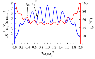
Figure 6: [Color online] Signal spectral photon-number density $n_{\rm s}^{\rm V}$ of volume SPDC (blue curve) and ratio $\eta_{\rm s}$ of the signal surface and volume photon-number densities (red curve) for the structure described in the caption to Fig. 5.

In time domain, the joint signal-idler probability densities $p^{\rm V}$, $p^{\rm S}$ and $p^{\rm SV}$ of detecting a signal photon at time $t_{\rm s}$ and its idler twin at time $t_{\rm i}$ attain typical cigar shapes in their topo graphs in the $t_{\rm s}-t_{\rm i}$ plane (for the probability density $p^{\rm SV}$, see Fig. 7). The joint photon-number probability densities $p^{\rm V}$ of volume SPDC and $p^{\rm S}$ of surface SPDC have similar profiles. Maximum of the probability density $p^{\rm V}$ ($p^{\rm S}$) is reached at $t\equiv t_{\rm s}=t_{\rm i}=10.3$ fs ($t=10.1$ fs). On the other hand, maximum of the probability density $p^{\rm SV}$ is observed earlier, at $t=9.5$ fs. This is the consequence of strong destructive interference between the volume and surface contributions to SPDC process. We note that this time gives relative average delay that a signal (as well as an idler) photon needs to leave the structure after being born ’inside’ the propagating pump pulse.

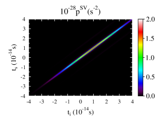
Figure 7: [Color online] Joint signal-idler probability density $p^{\rm SV}$ of the complete SPDC process as it depends on the signal- ($t_{\rm s}$) and idler-photon ($t_{\rm i}$) detection times.

The profiles of conditional probabilities $p^{\rm S}$, $p^{\rm V}$ and $p^{\rm SV}$ of detecting a signal photon at time $t_{\rm s}$ provided that its idler twin was detected at time $t_{\rm i}$ are close to each other. They are drawn for the analyzed structure in Fig. 8 for $t_{\rm i}=10$ fs, where their widths equal 1.4 fs (FWHM).

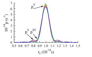
Figure 8: [Color online] Conditional probability densities $p^{\rm SV}$ (complete SPDC, blue curve), $p^{\rm V}$ (volume SPDC, green) and $p^{\rm S}$ (surface SPDC, red) of detecting a signal photon at time $t_{\rm s}$ provided that its idler photon was detected at time $t_{\rm i}=10$ fs.

Also the signal-field photon fluxes $p_{s}^{\rm S}$, $p_{s}^{\rm V}$ and $p_{s}^{\rm SV}$ are close to each other, as documented in Fig. 9. Their roughly Gaussian temporal profiles are 35.8 fs wide (FWHM), which is comparable to the pump-beam temporal width.

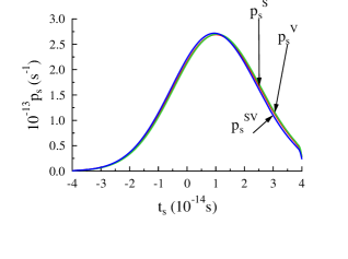
Figure 9: [Color online] Signal-field photon fluxes $p_{\rm s}^{\rm SV}$ (complete SPDC, blue curve), $p_{\rm s}^{\rm V}$ (volume SPDC, green) and $p_{\rm s}^{\rm S}$ (surface SPDC, red).

In the analyzed structure, photons comprising the generated photon pairs may leave the structure in both forward and backward directions and also in different polarization combinations. The total number $N^{\rm SV}$ of photon pairs leaving the structure at both directions is $2.9\times 10^{-3}$ mm^-2 per pulse. Whereas the volume SPDC process would alone provide $N^{\rm V}=6.9\times 10^{-3}$ mm^-2 photon pairs per pulse, the surface SPDC process alone would generate $N^{\rm S}=4.1\times 10^{-3}$ mm^-2 photon pairs per pulse. This means that the efficiency of surface SPDC reaches around 60 % of that of volume SPDC. We note that the absolute photon-pair generation rates reached in the analyzed structure are comparable in the magnitude with those characterizing a perfectly phase-matched structure containing the same amount of nonlinear GaN material as the analyzed structure (for more details, see Peřina Jr. (2011)).

V Conclusion

The model of complete spontaneous parametric down-conversion comprising both its volume and surface contributions has been developed for 1D nonlinear layered structures considering simultaneously the solution of Heisenberg equations in individual layers and continuity requirements of the field’s amplitudes at the layers’ boundaries. The analysis of fields’ propagation around the boundaries has allowed to clearly separate the volume and surface contributions to the nonlinear process. Strong destructive interference of the fields’ amplitudes arising in the volume and surface nonlinear processes has been observed. Owing to this interference, the photon-pair generation rates equal around one half of those that would be generated in the only volume nonlinear process. The surface nonlinear process is in general weaker than that in the volume, but both of them are comparably strong in the spectral regions with lower efficiencies of photon-pair generation.

VI Acknowledgements

The authors acknowledge project no. 15-08971S of GAČR and project no. LO1305 of MŠMT ČR for support.

References

- Louisell et al. (1961) W. H. Louisell, A. Yariv, and A. E. Siegman, “Quantum fluctuations and noise in parametric processes. I.” Phys. Rev. 124, 1646–1654 (1961).
- Harris et al. (1967) S. E. Harris, M. K. Oshman, and R. L. Byer, “Observation of tunable optical parametric fluorescence,” Phys. Rev. Lett. 18, 732–734 (1967).
- Magde and Mahr (1967) D. Magde and H. Mahr, “Study in ammonium dihydrogen phosphate of spontaneous parametric interaction tunable from 4400 to 16 000 A,” Phys. Rev. Lett. 18, 905–907 (1967).
- Keller and Rubin (1997) T. E. Keller and M. H. Rubin, “Theory of two-photon entanglement for spontaneous parametric down-conversion driven by a narrow pump pulse,” Phys. Rev. A 56, 1534–1541 (1997).
- Svozilík et al. (2012) J. Svozilík, J. Peřina Jr., and J. P. Torres, “High spatial entanglement via chirped quasi-phase-matched optical parametric down-conversion,” Phys. Rev. A 86, 052318 (2012).
- Grice et al. (2008) W. P. Grice, R. S. Bennink, Z. Zhao, K. Meyer, W. Whitten, and R. Shaw, “Spectral and spatial effects in spontaneous parametric down-conversion with a focused pump,” in Quantum Communications and Quantum Imaging VI, SPIE Conference Series, Vol. 7092, edited by R. E. Meyers, Y. Shih, and K. S. Deacon (SPIE, Bellingham, 2008) p. 70920Q.
- Javůrek et al. (2014) D. Javůrek, J. Svozilík, and J. Peřina, “Emission of orbital-angular-momentum-entangled photon pairs in a nonlinear ring fiber utilizing spontaneous parametric down-conversion,” Phys. Rev. A 90, 043844 (2014).
- Peřina Jr. et al. (2009a) J. Peřina Jr., A. Lukš, O. Haderka, and M. Scalora, “Surface spontaneous parametric down-conversion,” Phys. Rev. Lett. 103, 063902 (2009a).
- Peřina Jr. (2014) J. Peřina Jr., “Spontaneous parametric down-conversion in nonlinear layered media,” in Progress in Optics, Vol. 59, edited by E. Wolf (Elsevier, Amsterdam, 2014) pp. 89–158.
- Boyd (2003) R. W. Boyd, Nonlinear Optics, 2nd edition (Academic Press, New York, 2003).
- Dmitriev et al. (1999) V. G. Dmitriev, G. G. Gurzadyan, and D. N. Nikogosyan, Handbook of Nonlinear Optical Crystals (Springer-Verlag, Berlin Heidelberg, 1999).
- Peřina Jr. et al. (2006) J. Peřina Jr., M. Centini, C. Sibilia, M. Bertolotti, and M. Scalora, “Properties of entangled photon pairs generated in one-dimensional nonlinear photonic-band-gap structures,” Phys. Rev. A 73, 033823 (2006).
- Peřina Jr. et al. (2009b) J. Peřina Jr., M. Centini, C. Sibilia, and M. Bertolotti, “Photon-pair generation in random nonlinear layered structures,” Phys. Rev. A 80, 033844 (2009b).
- Peřina Jr. (2011) J. Peřina Jr., “Spatial properties of entangled photon pairs generated in nonlinear layered structures,” Phys. Rev. A 84, 053840 (2011).
- Javurek et al. (2012) D. Javurek, J. Svozilík, and J. Peřina Jr., “Entangled photon-pair generation in metallo-dielectric photonic bandgap structures,” in Wave and Quantum Aspects of Contemporary Optics, SPIE Conference proceedings, Vol. 8697, edited by J. Peřina Jr., L. Nožka, M. Hrabovský, D. Senderáková, W. Urbanczyk, and O. Haderka (SPIE, Bellingham, 2012).
- Javurek et al. (2014) D. Javurek, J. Svozilík, and J. Peřina Jr., “Spontaneous parametric down conversion in nonlinear metal-dielectric layered media,” in Wave and Quantum Aspects of Contemporary Optics, SPIE Conference proceedings, Vol. 9441, edited by A. Popio³ek-Masajada and W. Urbańczyk (SPIE, Bellingham, 2014) p. 94410V.
- Zhu et al. (2012) E. Y. Zhu, Z. Tang, L. Qian, L. G. Helt, M. Liscidini, J. E. Sipe, C. Corbari, A. Canagasabey, M. Ibsen, and P. G. Kazansky, “Direct generation of polarization-entangled photon pairs in a poled fiber,” Phys. Rev. Lett. 108, 213902 (2012).
- Javůrek et al. (2014a) D. Javůrek, J. Svozilík, and J. Peřina Jr., “Proposal for the generation of photon pairs with nonzero orbital angular momentum in a ring fiber,” Opt. Express 22, 23743–23748 (2014a).
- Eckstein et al. (2011) A. Eckstein, A. Christ, P. J. Mosley, and C. Silberhorn, “Highly efficient single-pass source of pulsed single-mode twin beams of light,” Phys. Rev. Lett. 106, 013603 (2011).
- Jachura et al. (2014) M. Jachura, M. Karpinski, C. Radzewicz, and K. Banaszek, “High-visibility nonclassical interference of photon pairs generated in a multimode nonlinear waveguide,” Opt. Express 22, 8624—8632 (2014).
- Machulka et al. (2013) R. Machulka, J. Svozilík, J. Soubusta, J. Peřina Jr., and O. Haderka, “Spatial and spectral properties of the pulsed second-harmonic generation in a PP-KTP waveguide,” Phys. Rev. A 87, 013836 (2013).
- Clausen et al. (2014) C. Clausen, F. Bussieres, A. Tiranov, H. Herrmann, C. Silberhorn, W. Sohler, M. Afzelius, and N. Gisin, “A source of polarization-entangled photon pairs interfacing quantum memories with telecom photons,” N. J. Phys. 16 (2014).
- Chen et al. (2014) L. Chen, P. Xu, Y. F. Bai, X. W. Luo, M. L. Zhong, M. Dai, M. H. Lu, and S. N. Zhu, “Concurrent optical parametric down-conversion in nonlinear photonic crystals,” Opt. Express 22, 13164–13169 (2014).
- Hayata and Koshiba (1991) K Hayata and M Koshiba, “Quasi-phase-matched multiwave mixing in a periodically poled ferroelectric crystal,” Opt. Lett. 16, 560–562 (1991).
- Lim et al. (1989) E. J. Lim, M. M. Fejer, and R. L. Byer, “2nd-harmonic generation of green light in periodically poled planar lithium-niobate wave-guide,” Electron. Lett. 25, 174–175 (1989).
- Shinozaki et al. (1992) K. Shinozaki, T. Fukunaga, K. Watanabe, and T. Kamijoh, “Automatic quasiphase matching for 2nd-harmonic generation in a periodically poled LiNbO3 wave-guide,” J. Appl. Phys. 71, 22–27 (1992).
- Kashyap (1991) R. Kashyap, “Phase-matched 2nd-harmonic generation in periodically poled optical fibers,” Appl. Phys. Lett. 58, 1233–1235 (1991).
- Chmela (1991) P. Chmela, “Preparation of optical fibers for effective 2nd-harmonic generation by the poling technique,” Opt. Lett. 16, 443–445 (1991).
- Harris (2007) S. E. Harris, “Chirp and compress: Toward single-cycle biphotons,” Phys. Rev. Lett. 98, 063602 (2007).
- Brida et al. (2009) G. Brida, M. V. Chekhova, I. P. Degiovanni, M. Genovese, G. Kh. Kitaeva, A. Meda, and O. A. Shumilkina, “Chirped biphotons and their compression in optical fibers,” Phys. Rev. Lett. 103, 193602 (2009).
- Svozilík and Peřina Jr. (2009) J. Svozilík and J. Peřina Jr., “Properties of entangled photon pairs generated in periodically poled nonlinear crystals,” Phys. Rev. A 80, 023819 (2009).
- Svozilík and Peřina Jr. (2011) J. Svozilík and J. Peřina Jr., “Intense ultra-broadband down-conversion from randomly poled nonlinear crystals,” in Nonlinear Optics and Applications V, SPIE Conference proceedings, Vol. 8071, edited by M. Bertolotti (SPIE, Bellingham, 2011) p. 807105.
- Bloembergen and Pershan (1962) N. Bloembergen and P. S. Pershan, “Light waves at the boundary of nonlinear media,” Phys. Rev. 128, 606–622 (1962).
- Bloembergen et al. (1969) N. Bloembergen, H. J. Simon, and C. H. Lee, “Total reflection phenomena in second-harmonic generation of light,” Phys. Rev. 181, 1261–1271 (1969).
- Mlejnek et al. (1999) M. Mlejnek, E. M. Wright, J. V. Moloney, and N. Bloembergen, “Second harmonic generation of femtosecond pulses at the boundary of a nonlinear dielectric,” Phys. Rev. Lett. 83, 2934–2937 (1999).
- Centini et al. (2008) M. Centini, V. Roppo, E. Fazio, F. Pettazzi, C. Sibilia, J. W. Haus, J. V. Foreman, N. Akozbek, M. J. Bloemer, and M. Scalora, “Inhibition of linear absorption in opaque materials using phase-locked harmonic generation,” Phys. Rev. Lett. 101, 113905 (2008).
- Peřina Jr. et al. (2009c) J. Peřina Jr., A. Lukš, and O. Haderka, “Emission of photon pairs at discontinuities of nonlinearity,” Phys. Rev. A 80, 043837 (2009c).
- Javůrek et al. (2014b) D. Javůrek, J. Svozilík, and J. Peřina, “Photon-pair generation in nonlinear metal-dielectric one-dimensional photonic structures,” Phys. Rev. A 90, 053813 (2014b).
- Huttner et al. (1990) B. Huttner, S. Serulnik, and Y. Ben-Aryeh, “Quantum analysis of light propagation in a parametric amplifier,” Phys. Rev. A 42, 5594—5600 (1990).
- Ben-Aryeh and Serulnik (1991) Y. Ben-Aryeh and S. Serulnik, “The quantum treatment of propagation in non-linear optical media by the use of temporal modes,” Phys. Lett. A 155, 473 – 479 (1991).
- Lukš et al. (2012) A. Lukš, V. Peřinová, and J. Křepelka, “Surface effect on spontaneous parametric down-conversion,” in Wave and Quantum Aspects of Contemporary Optics, SPIE Conference proceedings, Vol. 8697, edited by J. Peřina Jr., L. Nožka, M. Hrabovský, D. Senderáková, and W. Urbańczyk (SPIE, Bellingham, 2012) p. UNSP 869726.
- Peřinová et al. (2013) V. Peřinová, A. Lukš, and J. Peřina Jr., “Quantization of radiation emitted at discontinuities of nonlinearity,” Phys. Scr. T153, 014050 (2013).
- Yeh (1988) P. Yeh, Optical Waves in Layered Media (Wiley, New York, 1988).