Predicting Patient State-of-Health using Sliding Window and Recurrent Classifiers
Abstract
Bedside monitors in Intensive Care Units (ICUs) frequently sound incorrectly, slowing response times and desensitising nurses to alarms (Chambrin, 2001), causing true alarms to be missed (Hug et al., 2011). We compare sliding window predictors with recurrent predictors to classify patient state-of-health from ICU multivariate time series; we report slightly improved performance for the RNN for three out of four targets.
1 Introduction
Intensive Care Units (ICUs) hold patients who need constant critical care, so it is essential that doctors are notified quickly of any change in the state of the patient through bedside monitoring. Imhoff and Fried (2009) found that only 23% of bedside alarms in ICU are clinically relevant, representing minimal improvement from a much earlier study (Lawless, 1994).
Georgatzis and Williams (2015), henceforth G&W (2015), proposed a model which accurately classifies a number of clinical interventions which obscure patient vital signs. They discriminatively model these interventions using a Random Forest which takes sliding windows over the vital signs as input. This is a classification task for multiple binary targets, with a classifier for each modelled factor. They incorporate this classification into a Linear Dynamical System to infer the unobscured vital signs of the patient by maintaining a continuous state.
We compare sliding window predictors such as Random Forests or Multilayer Perceptrons (MLPs) with recurrent predictors such as Recurrent Neural Networks (RNNs). The aim is to not only compare how they perform, but also to understand how they approach the problem by investigating the solutions that they have learned. Sliding window predictors and recurrent predictors work in fundamentally different ways. Sliding window predictors make an independence assumption between each window, whereas recurrent predictors maintain dependence between the current timestep and all previous timesteps, prioritising more recent input. Gated RNN cells such as Long Short-Term Memory (LSTMs) (Hochreiter and Schmidhuber, 1997) and Gated Recurrent Unit (GRUs) (Chung et al., 2014) relax this independence assumption by learning to forget. They are effectively taking a sliding window over the data which they learn to adapt in length and structure in response to the input they receive. In this way, they may be able to capture longer-term dependencies than a sliding window predictor. We will show that the relaxation of the independence assumption is beneficial for the classification of ICU time series.
The sequence lengths for the recurrent predictor are unusually large at up to 153,678 timesteps. Related work from Lipton et al. (2015) uses sequences of up to around length 5,000 and Che et al. (2016) use sequences of up to length 150. In the broader RNN literature, Pouget-Abadie et al. (2014) report issues with sequences of over length 100 for neural machine translation and Le et al. (2015) report difficulty with sequences of length greater than 300. They rely on capturing the entirety of the dynamics of the input sequence in the hidden state, which limits the length of the sequences that can be processed. Additionally, gated RNN cells mitigate the vanishing gradient problem (Bengio et al., 1994) by learning to forget. We take a different approach, more akin to Zaremba et al. (2015), where we output the classification at each timestep.
To the best of our knowledge this is the first example of using RNNs to classify ICU multivariate time series at every timestep. Other related work (e.g. Lipton et al., 2015; Che et al., 2016) generates a single label to represent the entire sequence once the whole input sequenced has been processed.
2 Experiments
Data
The dataset for these experiments is as used by Lal et al. (2015). It incorporates twenty-seven adults admitted to the Neuro ICU at the Southern General Hospital in Glasgow. Information from four different channels was collected: electrocardiogram (ECG), systolic and diastolic arterial blood pressure (ABP), and systolic intracranial pressure (ICP). Lal et al. (2015) downsampled the readings to 1Hz, as this was shown by Quinn et al. (2009) to be sufficient for ICU time series classification. The explicitly modelled factors are stable periods (lack of annotations), blood samples (BS), endotracheal suctioning (SC), and damped traces (DT). All other annotations were grouped into an ‘X factor’. The dataset is discussed in more detail by Lal et al. (2015).
Sliding window predictor
For the sliding window predictor, we trained an MLP. We followed G&W (2015) by extracting a number of clinically-inspired features: least squared fits of a line of segments of the traces, an exponentially weighted moving average, the difference between the systolic and diastolic blood pressure channels (pulse pressure), and the first order differences of the sequences.The pulse pressure is important for detecting the damped trace event. We therefore normalised the blood pressure channels together by taking the mean and standard deviations for both channels combined. We then subtracted this overall mean from both channels and divided both channels by the overall standard deviation. This meant that systolic ABP was generally positive and diastolic ABP was generally negative. The heart rate (HR) and ICP channels were normalised individually using the same process. We supplied only the ABP channels to the blood sample and damped trace predictors, and all channels in other cases.
We included a layer with linear activation functions and initially set the weights to extract the G&W features (see McCarthy (2016) for weights after backpropagation). To operate on segments of the input sequence, connections were removed as necessary. This fed into a number of Rectified Linear Unit (ReLU) layers and finally, a sigmoid output layer trained to output , where is the modelled factor at time and is a sliding window over the input, where is the amount of past context and is the amount of future context.
Recurrent predictor
The recurrent predictor was composed of GRU hidden cells connected to a single sigmoid output unit. We used GRU cells instead of LSTMs as their simpler structure made them easier to analyse. Chung et al. (2014) demonstrated their performance was comparable over a range of problems. We trained using Truncated Backpropagation-Through-Time (Graves, 2013), with a length of 256 timesteps to make computation tractable. To investigate whether a recurrent predictor could learn long term correlations in the input, we directly supplied the input channels instead of extracting features. The Diastolic ABP was supplied to both the blood pressure and damped trace factors. For the blood sample factor we supplied the Systolic ABP and for the damped trace factor we supplied the pulse pressure. We did not supply the Systolic ABP to the damped trace factor in order to avoid multicollinearity. For the remaining factors, we supplied all channels.
We found with the MLP that including future context, , of up to 10 seconds improved classification, in keeping with G&W (2015). We therefore delayed the targets by 10 seconds during training to mirror this. Because gated RNN cells learn to forget, they are effectively learning a sliding window, but unlike sliding window predictors they adapt the size and structure of the sliding window based on the input they receive. Hyperparameter selection can learn an optimal sliding window length for a sliding window predictor, but it cannot adapt the sliding window structure to the extent that a gated RNN cell can.
Methodology
We trained both models using nested cross-validation (Varma and Simon, 2006) to compare their overall performance. In our case, this involves performing 3-fold cross-validation in an outer loop and then performing leave-one-patient-out cross-validation on each fold as an inner loop. We perform hyperparameter selection in this inner loop and then assess performance with the optimal hyperparameters on the test set from the outer loop. This ensures that hyperparameter selection and performance assessment occurs on different data. Varma and Simon (2006) found that cross-validation optimistically biases reported accuracy, whereas nested cross-validation reduces this bias. We evaluate the models by plotting Receiver Operating Characteristic curves on the concatenation of predictions in the three test sets and then compute the area under the curve.
We performed Early Stopping in all of the experiments. Every five epochs we calculated the cost on the validation set and compared with the cost five epochs prior. If the validation cost worsened on two successive occasions, we restored the weights which produced the minimum validation cost and terminated training. We did not use other regularisation techniques such as Dropout (Srivastava et al., 2014) because applications of Dropout to RNNs (e.g Zaremba et al., 2015; Krueger and Memisevic, 2016) are relatively novel and less well understood. We used the Adam optimisation routine of Kingma and Ba (2015) in all cases.
The input sequences were sparse, with only a small proportion of timesteps containing annotations. This class imbalance would make training difficult, so we used the annotated events as input sequences. However, we ensured that events from the same patient were never in the training and test set. These produced an even distribution of classes, including stable periods. We included context information of length equal to the event on either side, under the assumption that this would contain stable periods.
Hyperparameter selection
These predictors have a number of hyperparameters which need to be set in order to create the optimal model. For the sliding window predictor, these were the number of hidden layers in , the number of hidden units (), the length of the segments and , and the learning rate (). The number of hidden units was equal for all hidden layers. For the recurrent predictor, we optimised the number of hidden cells in each layer () and the learning rate (). We include optimal hyperparameters in Appendix A.
G&W (2015) performed a grid search over hyperparameters, but neural networks contain many more hyperparameters than random forests. Instead, we used Bayesian optimisation by fitting a Gaussian Process prior over our observations and generating new hyperparameters using an acquisition function which computes the expected improvement (Snoek et al., 2012, 2014; Gelbart et al., 2014). This improved the selection time considerably.
3 Results
In this section we will first report overall performance and then investigate the solutions learned by the models in order to interpret how they have learned.
| AUC | BS | DT | SC | X |
|---|---|---|---|---|
| DSLDS (Lal et al., 2015) | ||||
| MLP | ||||
| RNN |
Performance
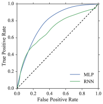
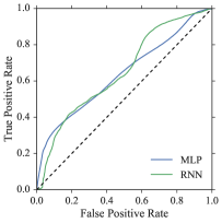
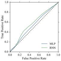
AUC scores for the MLP and RNN on the Adult ICU Dataset from Lal et al. (2015) are shown in Table 1 and ROC curves are included in Figure 1. The MLP and the random forest used by Lal et al. (2015) show very similar performance. The RNN achieved slightly improved results for the Blood Sample, Suction Event and X Factors.
The RNN could not match the performance of the MLP on damped traces and we have a number of hypotheses to explain this. The first is that the largest RNN we could run on one GPU had 128 hidden cells, whereas the largest MLP has 2048 hidden units. Whilst this is fine for temporal correlations, as the RNN hidden states are maintained through each timestep which gives it significantly more parameters, only the candidate activation can capture the pulse pressure at each timestep. Additionally, much of this information is lost when it passes through the update gate. Another possibility is that the damped trace sequences, at 153,678 timesteps long (42 hours), are too long for the RNN to fully capture their dynamics. They may vary through the period due to factors such as medical interventions or circadian rhythm. In comparison, the longest sequences for the Blood Sample, Endotracheal Suction and X factor sequences were 1,149 timesteps (19 mins), 13,176 timesteps (3.65 hrs), and 49,740 timesteps (13.81 hrs) respectively. Finally, we postulate in Section 4 that the RNNs are better at adapting to the baseline physiology of the patient. This can cause them to not classify some timesteps as damped traces, even if the annotations indicate that that they are.
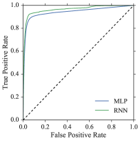
a) Blood Sample
b) Damped Trace
c) Suction Event
d) X
4 Discussion
To investigate how the predictors learned, we plotted the predictions, saliency maps between the input and the output (Mørch et al., 1995), and saliency maps between the activations (Erhan et al., 2009). Empirically, we made the following observations, which could warrant further study (see McCarthy (2016) sections 4 and 5 for further details).
Adapting to baseline physiology
Sliding window predictors incorrectly classify low pulse pressures as damped traces, whereas recurrent predictors wait for a reduction in pulse pressure before making a classification. This is important in ICU due to high vital sign variability between patients.
Classifying long-term events
Events are often obscured by other pathology. RNNs can maintain state through these disturbances, whereas sliding window predictors will often only classify the beginning and end of long events. However, this state maintenance can cause RNN hidden states to decay too slowly when events finish if they are not well delineated.
Noisy input sequences
The RNN was better at handling very volatile input because the hidden state causes the predictions to effectively be smoothed, in comparison to the MLP which produces very volatile predictions in response to this volatility.
Computational complexity
RNNs are much more computationally expensive to train. It is necessary to zero pad the sequences to the length of the longest sequence if one wishes to use a BLAS library with a batch size greater than one. Time spent processing zeros is wasted and their activations consume GPU RAM, limiting the size of models which can be trained. Solutions to this include using a smaller batch size, sacrificing parallelism, or multiplying sparse matrices which is slow. Sequences could also be segmented, improving parallelism at the cost of not capturing long-term dependencies.
5 Conclusion
In this report we have trained MLP and RNNs to compare sliding window and recurrent predictors in the classification of ICU time series. G&W (2015) built an ensemble of two sliding window predictors: the FSLDS and DSLDS, which improved performance compared to the individual models. Adding a recurrent predictor to this mixture may improve these results further.
We hope that the insight into how the models learn to approach the problem gained in this report will help the construction of better bedside alarms for the ICU in the future. Ideally any follow up to Lawless (1994) and Imhoff and Fried (2009) will find that the wolves are no longer crying.
Acknowledgements: The work of CW is supported in part by EPSRC grant EP/N510129/1.
References
- Bengio et al. (1994) Y. Bengio, P. Simard, and P. Frasconi. Learning Long-Term Dependencies with Gradient Descent is Difficult. IEEE Transactions on Neural Networks, 5(2):157–166, 1994. ISSN 19410093. doi: 10.1109/72.279181.
- Chambrin (2001) M. C. Chambrin. Alarms in the intensive care unit: how can the number of false alarms be reduced? Critical Care, 5(4):184–188, 2001. ISSN 1364-8535. doi: 10.1186/cc1021.
- Che et al. (2016) Z. Che, S. Purushotham, K. Cho, D. Sontag, and Y. Liu. Recurrent Neural Networks for Multivariate Time Series with Missing Values. arXiv:1606.01865, 2016.
- Chung et al. (2014) J. Chung, C. Gulcehre, K. Cho, and Y. Bengio. Empirical Evaluation of Gated Recurrent Neural Networks on Sequence Modeling. arXiv:1412.3555v1, pages 1–9, 2014.
- Erhan et al. (2009) D. Erhan, A. Courville, Y. Bengio, and P. Vincent. Visualizing Higher Layer Features of a Deep Network. Technical Report 1341, DIRO, Universite de Montreal, 2009.
- Gelbart et al. (2014) M. A. Gelbart, J. Snoek, and R. P. Adams. Bayesian Optimization with Unknown Constraints. arXiv:1403.5607v1, pages 1–14, 2014. ISSN 1098-6596. doi: 10.1017/CBO9781107415324.004.
- Georgatzis and Williams (2015) K. Georgatzis and C. K. I. Williams. Discriminative Switching Linear Dynamical Systems applied to Physiological Condition Monitoring. Proceedings of Uncertainty in AI, 2015.
- Graves (2013) A. Graves. Generating sequences with recurrent neural networks. arXiv:1308.0850, pages 1–43, 2013. ISSN 18792782. doi: 10.1145/2661829.2661935.
- Hochreiter and Schmidhuber (1997) S. Hochreiter and J. Schmidhuber. Long Short-Term Memory. Neural Computation, 9(8):1735–1780, 1997. ISSN 0899-7667. doi: 10.1162/neco.1997.9.8.1735.
- Hug et al. (2011) C. W. Hug, G. D. Clifford, and A. T. Reisner. Clinician blood pressure documentation of stable intensive care patients: an intelligent archiving agent has a higher association with future hypotension. Critical Care Medicine, 39(5):1006–14, 2011. doi: 10.1097/CCM.0b013e31820eab8e.
- Imhoff and Fried (2009) M. Imhoff and R. Fried. The crying wolf: Still crying? Anesthesia and Analgesia, 108(5):1382–1383, 2009. ISSN 00032999. doi: 10.1213/ane.0b013e31819ed484.
- Kingma and Ba (2015) D. Kingma and J. Ba. Adam: A Method for Stochastic Optimization. In International Conference on Learning Representations, pages 1–13, 2015.
- Krueger and Memisevic (2016) D. Krueger and R. Memisevic. Regularizing RNNs by Stabilizing Activations. ICLR, pages 1–8, 2016.
- Lal et al. (2015) P. Lal, C. K. I. Williams, G. Konstantinos, P. Hawthorne, C. McMonagle, I. Piper, and M. Shaw. Detecting Artifactual Events in Vital Signs Monitoring Data. Technical report, University of Edinburgh and University of Glasgow, 2015.
- Lawless (1994) S. T. Lawless. Crying wolf: false alarms in a pediatric intensive care unit., 1994. ISSN 0090-3493.
- Le et al. (2015) Q. V. Le, N. Jaitly, and G. E. Hinton. A Simple Way to Initialize Recurrent Networks of Rectified Linear Units. arXiv:1504.00941, 2015.
- Lipton et al. (2015) Z. C. Lipton, D. C. Kale, C. Elkan, and R. Wetzell. Learning to Diagnose with LSTM Recurrent Neural Networks. In ICLR, pages 1–18, 2015.
- McCarthy (2016) A. McCarthy. An Evaluation of Sliding Window and Recurrent Predictors for the Classification of ICU Time Series. MSc dissertation. University of Edinburgh. 2016.
- Mørch et al. (1995) N. J. S. Mørch, U. Kjems, L. K. Hansen, C. Svarer, I. Law, B. Lautrup, S. C. Strother, and K. Rehm. Visualization of Neural Networks Using Saliency Maps. In Proceedings of 1995 IEEE International Conference on Neural Networks, volume 4, pages 2085–2090, 1995. ISBN 0-7803-2768-3. doi: 10.1109/ICNN.1995.488997.
- Pouget-Abadie et al. (2014) J. Pouget-Abadie, D. Bahdanau, B. van Merrienboer, K. Cho, and Y. Bengio. Overcoming the Curse of Sentence Length for Neural Machine Translation using Automatic Segmentation. arXiv:1409.1257, 2014.
- Quinn et al. (2009) J. A. Quinn, C. K. Williams, and N. McIntosh. Factorial Switching Linear Dynamical Systems Applied to Physiological Condition Monitoring. IEEE Transactions on Pattern Analysis and Machine Intelligence, 31(9):1537–1551, 2009. ISSN 0162-8828. doi: 10.1109/TPAMI.2008.191.
- Snoek et al. (2012) J. Snoek, H. Larochelle, and R. P. Adams. Practical Bayesian Optimization of Machine Learning Algorithms. In F. Pereira, C. J. C. Burges, L. Bottou, and K. Q. Weinberger, editors, Advances in Neural Information Processing Systems 25, pages 2951–2959. Curran Associates, Inc., 2012.
- Snoek et al. (2014) J. Snoek, K. Swersky, R. S. Zemel, and R. P. Adams. Input Warping for Bayesian Optimization of Non-Stationary Functions. In ICML, pages 1674–1682, 2014.
- Srivastava et al. (2014) N. Srivastava, G. E. Hinton, A. Krizhevsky, I. Sutskever, and R. Salakhutdinov. Dropout : A Simple Way to Prevent Neural Networks from Overfitting. Journal of Machine Learning Research (JMLR), 15:1929–1958, 2014. ISSN 15337928. doi: 10.1214/12-AOS1000.
- Varma and Simon (2006) S. Varma and R. Simon. Bias in Error Estimation when using Cross-Validation for Model Selection. BMC Bioinformatics, 7:91, 2006. ISSN 1471-2105. doi: 10.1186/1471-2105-7-91.
- Zaremba et al. (2015) W. Zaremba, I. Sutskever, and O. Vinyals. Recurrent Neural Network Regularization. ICLR, pages 1–8, 2015.
Appendix A Optimal hyperparameters
| Factor | Outer Fold | ||
|---|---|---|---|
| 1 | |||
| BS | 2 | ||
| 3 | |||
| 1 | |||
| DT | 2 | ||
| 3 | |||
| 1 | |||
| SC | 2 | ||
| 3 | |||
| 1 | |||
| X | 2 | ||
| 3 |
| Factor | Outer Fold | ||||
|---|---|---|---|---|---|
| 1 | |||||
| BS | 2 | ||||
| 3 | |||||
| 1 | |||||
| DT | 2 | ||||
| 3 | |||||
| 1 | |||||
| SC | 2 | ||||
| 3 | |||||
| 1 | |||||
| X | 2 | ||||
| 3 |