A Stable and High-Order Accurate Discontinuous Galerkin Based Splitting Method for the Incompressible Navier-Stokes Equations

Abstract

In this paper we consider discontinuous Galerkin (DG) methods for the incompressible Navier-Stokes equations in the framework of projection methods. In particular we employ symmetric interior penalty DG methods within the second-order rotational incremental pressure correction scheme. The major focus of the paper is threefold: i) We propose a modified upwind scheme based on the Vijayasundaram numerical flux that has favourable properties in the context of DG. ii) We present a novel postprocessing technique in the Helmholtz projection step based on $H(\text{div})$ reconstruction of the pressure correction that is computed locally, is a projection in the discrete setting and ensures that the projected velocity satisfies the discrete continuity equation exactly. As a consequence it also provides local mass conservation of the projected velocity. iii) Numerical results demonstrate the properties of the scheme for different polynomial degrees applied to two-dimensional problems with known solution as well as large-scale three-dimensional problems. In particular we address second-order convergence in time of the splitting scheme as well as its long-time stability.

todoenv[1][]

1 Introduction

The application of discontinuous Galerkin (DG) methods to the Navier-Stokes equations is popular due to their potentially high order of convergence, the inf-sup stability and local mass conservation property [1, 2, 3]. The latter is generally not fulfilled for conforming finite element discretizations. In addition to the $2\times 2$ block structure arising from the saddle point system discontinuous Galerkin methods offer a further block structure when the unknowns associated with one cell of the mesh are grouped together. This data structure is essential for high-performance implementations of the discontinuous Galerkin method [4, 5] as it avoids costly memory gather and scatter operations when compared to conforming finite element methods.

Operator splitting methods for solving the instationary Navier-Stokes equations has been subject to detailed investigations for the recent decades. One possibility in the splitting methods is to split between the convective term and the saddle point structure which is realized in Glowinski’s $\Theta$-scheme, [6, 7]. Another possibility is to split between incompressibility and dynamics which has been independently developed by Chorin [8] and Témam [9] and is referred to as Chorin’s projection method. The latter splitting schemes have the appealing feature that at each time step, instead of solving a saddle point system, one only has to solve a vector-valued heat equation for the velocity (in the Stokes case) and a Poisson equation for the pressure. The choice of artificial boundary conditions on the pressure Poisson equation is a delicate issue in projection methods of this class [10, 11, 12]. Several higher-order extensions of Chorin’s first order method have been suggested in the literature [13, 14, 15, 16, 17, 18]. Here we concentrate on the classic incremental pressure-correction scheme (IPCS) [19] and the rotational incremental pressure-correction scheme (RIPCS) [14].

The use of a DG spatial discretization within splitting schemes is a current subject of active research. A naive computation of the divergence free velocity by subtraction of the rotation free part is reported to be unstable when the spatial mesh is coarse and the time step is small, see [20, 21, 4], where several local postprocessing techniques are discussed to overcome this difficulty. In this paper we propose a new postprocessing technique based on $H(\text{div})$ reconstruction of the discrete pressure gradient which is popular in porous media flow computations [22, 23]. The new approach provides a discrete velocity that satisfies the discrete continuity equation exactly and in consequence is locally mass conservative and defines a projection. These properties are not satisfied by the postprocessing schemes available in the literature.

The structure of the paper is organized as follows: In section 2 we recapitulate the discontinuous Galerkin discretization by the interior penalty method as presented in [2, 1]. In section 3 we discuss the Helmholtz decomposition, prove our main result and present the projection methods In section 4 we elaborate on numerical experiments for the discontinuous Galerkin discretization based on the reference problems by [15, 16, 24, 18] and assess the properties of the new postprocessing scheme.

2 Discontinuous Galerkin discretization of the incompressible Navier-Stokes equations

In this section we present the spatial discretization of the Navier-Stokes system with an interior penalty DG method taken from [2]. The convective term is discretized using the Vijayasundaram flux.

The instationary incompressible Navier-Stokes equations in an open and bounded domain $\Omega\subset\mathbb{R}^{d}$ ($d=2,3$) determining the velocity $v$ and pressure $p$ for a right-hand side $f$, constant viscosity $\mu$ and density $\rho$ are given by

$$\rho\partial_{t}v-\mu\Delta v+\rho(v\cdot\nabla)v+\nabla p =f \textup{in}\;\Omega\times(0,T]$$ (1a)

$$\nabla\cdot v =0 \textup{in}\;\Omega\times(0,T]$$ (1b)

$$v =v_{0} \textup{for}\;t=0$$ (1c)

and either Dirichlet boundary condition for the velocity:

$$v =g \textup{on}\;\Gamma_{D}=\partial\Omega,t\in(0,T]$$ (1d)

together with

$$\int_{\Omega}p\mathrm{d}x =0 \textup{for all}\;t\in(0,T]$$ (1e)

or mixed boundary conditions:

$$v =g \textup{on}\;\Gamma_{D}\neq\{\partial\Omega,\emptyset\}$$ (1f)

$$\mu\nabla vn-pn =0 \textup{on}\;\Gamma_{N}=\partial\Omega\setminus\Gamma_{D}$$ (1g)

with $(0,T]$ being the time interval of interest. For pure Dirichlet boundary conditions $g$ is required to satisfy the compatibility condition $\int_{\partial\Omega}g\cdot n\mathrm{d}x=0$. In the numerical examples below we will also consider periodic boundary conditions in addition. Under appropriate assumptions the Navier-Stokes problem in weak form has a solution $(v,p)$ in $(H^{1}(\Omega))^{d}\times L^{2}(\Omega)$ for $t\in(0,T]$, [25, 26]. In case of pure Dirichlet boundary conditions the pressure is only determined up to a constant and is in the space $L^{2}_{0}(\Omega)=\{q\in L^{2}(\Omega)\mid\int_{\Omega}q\mathrm{d}x=0\}$.

For the discretization let $\mathcal{E}_{h}$ be an affine cubic mesh (the restriction to affine meshes is only needed when the Raviart-Thomas reconstruction is used) with maximum diameter $h$. We denote by $\Gamma_{h}^{\mathrm{int}}$ the set of all interior faces, by $\Gamma_{h}^{D}$ the set of all faces intersecting with the Dirichlet boundary $\Gamma_{D}$ and by $\Gamma_{h}^{N}$ the set of all faces intersecting with the mixed boundary $\Gamma_{N}$. We set $\Gamma_{h}=\Gamma_{h}^{\mathrm{int}}\cup\Gamma_{h}^{D}\cup\Gamma_{h}^{N}$. To an interior face $e\in\Gamma_{h}^{\mathrm{int}}$ shared by elements $E_{e}^{1}$ and $E_{e}^{2}$ we define an orientation through its unit normal vector $n_{e}$ pointing from $E_{e}^{1}$ to $E_{e}^{2}$. The jump and average of a scalar-valued function $\phi$ on a face is then defined by

$$[\phi] =\phi\mid_{E_{e}^{1}}-\phi\mid_{E_{e}^{2}}\quad\;=\phi^{\mathrm{int}}-\phi^{\mathrm{ext}},$$ (2)

$$\{\phi\} =\frac{1}{2}\phi\mid_{E_{e}^{1}}+\frac{1}{2}\phi\mid_{E_{e}^{2}}=\frac{1}{2}\phi^{\mathrm{int}}+\frac{1}{2}\phi^{\mathrm{ext}}\;.$$

Note that the definition of jump and average can be extended in a natural way to vector and matrix-valued functions. If $e\in\partial\Omega$ then $n_{e}$ corresponds to the outer normal vector $n$. Below we make heavy use of the identities and notation, respectively:

$$[uv] =[u]\{v\}+\{u\}[v]\;, (u,v)_{0,\omega} =\int_{\omega}uv\,dx\;, u,v$$ ( scalar-valued) (3)

$$[u\cdot v] =[u]\cdot\{v\}+\{u\}\cdot[v]\;, (u,v)_{0,\omega} =\int_{\omega}u\cdot v\,dx\;, u,v$$ ( vector-valued)

$$[u:v] =[u]:\{v\}+\{u\}:[v]\;, (u,v)_{0,\omega} =\int_{\omega}u:v\,dx\;, \text{($u,v$ matrix-valued)}.$$

The DG discretization on cuboid meshes is based on the non-conforming finite element space of polynomial degree $p$

$$Q_{h}^{p}=\{v\in L^{2}(\Omega)\mid v|_{E}=q\circ\mu_{E}^{-1},q\in\mathbb{Q}_{p,d},E\in\mathcal{E}_{h}\}$$ (4)

where $\mu_{E}:\hat{E}\to E$ is the transformation from the reference cube $\hat{E}$ to $E$ and $\mathbb{Q}_{p,d}$ is the set of polynomials of maximum degree $p$ in $d$ variables. The approximation spaces for velocity and pressure are then

$$X^{p}_{h}\times M_{h}^{p-1} =(Q_{h}^{p})^{d}\times(Q_{h}^{p-1}\cap L^{2}_{0}(\Omega)) \text{(Dirichlet b. c.)},$$ (5a)

$$X^{p}_{h}\times M_{h}^{p-1} =(Q_{h}^{p})^{d}\times Q_{h}^{p-1} \text{(mixed b. c.)}.$$ (5b)

We make use of the following mesh-dependent forms defined on $X_{h}^{p}\times X_{h}^{p}$, $X_{h}^{p}\times M_{h}^{p-1}$ and $M_{h}^{p-1}$, respectively:

$$a(u,v) =d(u,v)+J_{0}(u,v),\ \text{where}$$ (6a)

$$d(u,v) =\sum_{E\in\mathcal{E}_{h}}(\nabla u,\nabla v)_{0,E}-\sum_{e\in\Gamma_{h}^{\mathrm{int}}}(\{\nabla u\}n_{e},[v])_{0,e}-\sum_{e\in\Gamma_{h}^{D}}(\nabla u^{\mathrm{int}}n_{e},v^{\mathrm{int}})_{0,e},$$ (6b)

$$J_{0}(u,v) =\epsilon\sum_{e\in\Gamma_{h}^{\mathrm{int}}}(\{\nabla v\}n_{e},[u])_{0,e}+\epsilon\sum_{e\in\Gamma_{h}^{D}}(\nabla v^{\mathrm{int}}n_{e},u^{\mathrm{int}})_{0,e}$$

$$\quad+\sum_{e\in\Gamma_{h}^{\mathrm{int}}}\frac{\sigma}{h_{e}}([u],[v])_{0,e}+\sum_{e\in\Gamma_{h}^{D}}\frac{\sigma}{h_{e}}(u^{\mathrm{int}},v^{\mathrm{int}})_{0,e},$$ (6c)

$$b(v,q) =-\sum_{E\in\mathcal{E}_{h}}(\nabla\cdot v,q)_{0,E}+\sum_{e\in\Gamma_{h}^{\mathrm{int}}}([v]\cdot n_{e},\{q\})_{0,e}+\sum_{e\in\Gamma_{h}^{D}}(v^{\mathrm{int}}\cdot n,q^{\mathrm{int}})_{0,e},$$ (6d)

$$l(v;t) =\sum_{E\in\mathcal{E}_{h}}(f(t),v)_{0,E}+\epsilon\sum_{e\in\Gamma_{h}^{D}}(\nabla v^{\mathrm{int}}n_{e},g(t))_{0,e}+\sum_{e\in\Gamma_{D}}\frac{\sigma}{h_{e}}(g(t),v^{\mathrm{int}})_{0,e},$$ (6e)

$$r(q;t) =\sum_{e\in\Gamma_{h}^{D}}(g(t)\cdot n,q^{\mathrm{int}})_{0,e}\;.$$ (6f)

Here we made the time dependence of the right hand side functionals explicit. For ease of writing this will be omitted mostly below. In the interior penalty parameter $\sigma/h_{e}$, the denominator accounts for the mesh dependence. The formula for $h_{e}$,

$$h_{e}=\begin{cases}\frac{\min\left(\left|E^{\mathrm{int}}(e)\right|,\left|E^{\mathrm{ext}}(e)\right|\right)}{\left|e\right|}&,E^{\mathrm{int}}(e)\cap E^{\mathrm{ext}}(e)=e\\ \frac{\left|E^{\mathrm{int}}(e)\right|}{\left|e\right|}&,E^{\mathrm{int}}(e)\cap\Gamma_{D}=e\end{cases}\;,$$

has been stated in [27] where it was proven that this choice ensures coercivity of the bilinear form for anisotropic meshes. For $\sigma$ we choose $\sigma=\alpha p(p+d-1)$ as in [28] with $\alpha$ a user-defined parameter. In $J_{0}$ the Symmetric Interior Penalty Galerkin (SIPG) ($\epsilon=-1$) method is preferred since the matrix of the linear system in absence of the convection term is then symmetric. Other choices are the NIPG ($\epsilon=1$) or IIPG ($\epsilon=0$) method.

A first discretization of the nonlinear term in the Navier-Stokes equations is the standard (or centered) discretization,

$$c(u;z,\theta)=\sum_{E\in\mathcal{E}_{h}}((u\cdot\nabla)z,\theta)_{0,E},$$ (7)

that lets us define the discrete in space, continuous in time formulation of the Navier-Stokes problem (1). Find $v_{h}(t):(0,T]\to X_{h}^{p}$, $p_{h}(t):(0,T]\to M_{h}^{p-1}$:

$$\rho(\partial_{t}v_{h},\varphi)_{0,\Omega}+\mu a(v_{h},\varphi)+\rho c(v_{h};v_{h},\varphi)+b(\varphi,p_{h}) =l(\varphi;t),$$ (8a)

$$b(v_{h},q) =r(q;t),$$ (8b)

for all $(\varphi,q)\in X_{h}^{p}\times M_{h}^{p-1}$. This formulation for the variational form $c$ is only applicable for small Reynolds numbers. Therefore we present for higher Reynolds numbers an upwind discretization in Section 2.1. The following observation will be used in several circumstances below.

Remark 1.

The bilinear form $b(v,q)$ has the equivalent representation

$$b(v,q)=\sum_{E\in\mathcal{E}_{h}}(v,\nabla q)_{0,E}-\sum_{e\in\Gamma_{h}^{\text{int}}}(\{v\}\cdot n_{e},[q])_{0,e}-\sum_{e\in\Gamma_{h}^{N}}(v\cdot n,q)_{0,e}.$$ (9)

This holds true for Dirichlet and mixed boundary conditions (in the former case just set $\Gamma_{h}^{N}=\emptyset$).

Proof.

Follows from integration by parts and (3). ∎

As a corollary we obtain the following local mass conservation property by testing (8b) with $q=\chi_{E}$, the characteristic function of element $E$, and using Remark 1:

$$\sum_{e\in\Gamma_{h}^{\text{int}}\cap\partial E}(\{v\}\cdot n_{e},1)_{0,e}+\sum_{e\in\Gamma_{h}^{N}\cap\partial E}(v\cdot n_{e},1)_{0,e}+\sum_{e\in\Gamma_{h}^{D}\cap\partial E}(g\cdot n,1)_{0,e}=0.$$ (10)

2.1 Upwind discretization of the convective part

For higher Reynolds numbers we employ a suitable upwind discretization based on the Vijayasundaram numerical flux adapted from DG methods for inviscid compressible flow [29, 30].

Note that due to $\nabla\cdot v=0$ the convective term in the momentum equations can be written equivalently as $(v\cdot\nabla)v=\nabla\cdot(v\otimes v)$ where

$$F(v)=v\otimes v=[v_{1}v,\ldots,v_{d}v]=[F_{1}(v),\ldots,F_{d}(v)]$$

is the convective flux matrix with columns $F_{k}(v)=v_{k}v$ and $\nabla_{v}F_{k}(v)=(v_{k}I+v\otimes e_{k})$. $I$ denotes the identity matrix and $(e_{k})_{i}=\delta_{ik}$ are the coordinate unit vectors. In order to derive the upwinding we consider the first order system

$$\partial_{t}v+\nabla\cdot F(v)=0$$

which is said to be hyperbolic if the matrix

$$P(v,n)=\sum_{k=1}^{d}n_{k}\nabla_{v}F_{k}(v)=(v\cdot n)I+v\otimes n$$

is real diagonalizable for all $v,n\in\mathbb{R}^{d}$ with $\|n\|=1$ [31]. This is indeed the case for $v\cdot n\neq 0$. When $v\cdot n=0$, $P(v,n)=v\otimes n$ has $d$ eigenvalues zero with a corresponding eigenspace $W_{n}^{\perp}=\{w:w\cdot n=0\}$ of dimension $d-1$.

When discretizing the conservative form of the convective terms with DG one uses element-wise integration by parts to arrive at

$$\begin{split}c(v;v,\varphi)&=(\nabla\cdot F(v),\varphi)_{0,\Omega}=\sum_{E\in\mathcal{E}_{h}}(\nabla\cdot F(v),\varphi)_{0,E}=-\sum_{E\in\mathcal{E}_{h}}(F(v),\nabla\varphi)_{0,E}+\sum_{E\in\mathcal{E}_{h}}(F(v)n,\varphi)_{0,\partial E}\\ &=-\sum_{E\in\mathcal{E}_{h}}(F(v),\nabla\varphi)_{0,E}+\sum_{e\in\Gamma_{h}^{\text{int}}}([F(v)n_{e}\cdot\varphi],1)_{0,e}+\sum_{e\in\Gamma_{h}^{D}\cup\Gamma_{h}^{N}}(F(v)n,\varphi)_{0,e}\end{split}$$

Now the flux in face normal direction $F(v)n_{e}$ needs to be replaced by a consistent and conservative numerical flux function $\hat{F}(v,n_{e})$ which we now derive. Since $F_{k}(v)=v_{k}v$ is homogeneous of degree 2 (i.e. $F_{k}(\alpha v)=\alpha^{2}F_{k}(v)$ for $\alpha$ a real number) it admits a representation

$$F_{k}(v)=\frac{1}{2}\nabla_{v}F_{k}(v)v$$

and therefore

$$F(v)n=\frac{1}{2}P(v,n)v=\frac{1}{2}[(v\cdot n)I+v\otimes n]v=:B_{\frac{1}{2}}(v)v\;.$$

Using the identity $(v\cdot n)v=(v\otimes n)v$ we see

$$F(v)n=B_{\beta}(v)v:=[(1-\beta)(v\cdot n)+\beta v\otimes n]v$$

for any $\beta\in[0,1]$. For $v\cdot n\neq 0$, $B_{\beta}(v,n)$ is real diagonalizable with eigenvalues $\lambda_{\beta,i}\in\mathbb{R}$ and a full set of right eigenvectors $r_{i}$, $\text{span}\{r_{1},\ldots,r_{d-1}\}=W_{n}^{\perp}$, $r_{d}=v$, admitting the decomposition

$$B_{\beta}(v,n)=B_{\beta}^{+}(v,n)+B_{\beta}^{-}(v,n),$$

where $B_{\beta}^{\pm}(v,n)=TD_{\beta}^{\pm}T^{-1}$, $T=[r_{1},\ldots,r_{d}]$, $D_{\beta}^{\pm}$ are diagonal matrices with $(D_{\beta}^{+})_{ii}=\max(0,\lambda_{\beta,i})$ and $(D_{\beta}^{-})_{ii}=\min(0,\lambda_{\beta,i})$ (all eigenvectors and eigenvalues depending on $v$ and $n$).

Following [30], in the DG scheme we employ the Vijayasundaram numerical flux given by

$$\hat{F}_{\beta}(v,n_{e})=B^{+}_{\beta}(\{v\},n_{e})v^{\text{int}}+B^{-}_{\beta}(\{v\},n_{e})v^{\text{ext}}\;.$$ (11)

Here the matrices $B_{\beta}^{\pm}(\{v\},n_{e})$ are not applied to $\{v\}$ and therefore $(\{v\}\cdot n)I$ and $\{v\}\otimes n$ act differently. The effect is shown by the following

Observation 1.

Assume $\{v\}\cdot n\neq 0$. Then the numerical flux (11) satisfies

$$\begin{split}\hat{F}_{\beta}(v,n_{e})&=(1-\beta)\left[\max(0,\{v\}\cdot n_{e})v^{\text{int}}+\min(0,\{v\}\cdot n_{e})v^{\text{ext}}\right]\\ &\quad+\beta[H(\{v\}\cdot n_{e})(v^{\text{int}}\cdot n_{e})+H(-\{v\}\cdot n_{e})(v^{\text{ext}}\cdot n_{e})]\{v\}\;.\end{split}$$

where $H(x)$ is the Heaviside function.

Proof.

We consider the interior part. The eigenvectors of $B_{\beta}(\{v\},n_{e})$ are $d-1$ vectors spanning $W_{n}^{\perp}$ and $\{v\}$ independent of $\beta\in[0,1]$. We can uniquely decompose

$$v^{\text{int}}=\left(v^{\text{int}}-\frac{v^{\text{int}}\cdot n_{e}}{\{v\}\cdot n_{e}}\{v\}\right)+\frac{v^{\text{int}}\cdot n_{e}}{\{v\}\cdot n_{e}}\{v\}=w+\alpha\{v\}$$

where $w\in W_{n}^{\perp}$. Now

$$\begin{split}B^{+}_{\beta}&(\{v\},n_{e})v^{\text{int}}=B^{+}_{\beta}(\{v\},n_{e})(w+\alpha\{v\})\\ &=(1-\beta)\max(0,\{v\}\cdot n_{e})w+\max(0,\{v\}\cdot n_{e})\alpha\{v\}\\ &=(1-\beta)\max(0,\{v\}\cdot n_{e})(v^{\text{int}}-\alpha\{v\})+\max(0,\{v\}\cdot n_{e})\alpha\{v\}\\ &=(1-\beta)\max(0,\{v\}\cdot n_{e})v^{\text{int}}+\beta\frac{\max(0,\{v\}\cdot n_{e})(v^{\text{int}}\cdot n_{e})}{\{v\}\cdot n_{e}}\{v\}\;.\end{split}$$

$B^{-}_{\beta}(\{v\},n_{e})v^{\text{ext}}$ can be treated in the same way. ∎

The observation shows that for $\beta>0$ the $v\otimes n_{e}$ part gives a contribution in the flux in the direction of $\{v\}$, i.e. a central flux which moreover might have the wrong sign since the signs of $\{v\}\cdot n_{e}$ and $v^{\text{int}}\cdot n_{e}$ or $v^{\text{ext}}\cdot n_{e}$ might differ since the DG velocity is not in $H(\text{div};\Omega)$. (Note, however, that the new projection scheme to be described below improves significantly on this point). Also note that the upwind decision is based on the average velocity which is locally mass conservative due to (10).

For these reasons we propose to employ $\beta=0$ in the numerical flux function, leading to the simple form:

$$\hat{F}_{e}(v,n_{e})=\left\{\begin{array}[]{ll}\max(0,\{v\}\cdot n_{e})v^{\text{int}}+\min(0,\{v\}\cdot n_{e})v^{\text{ext}}&e\in\Gamma_{h}^{\text{int}}\\ \max(0,v^{\text{int}}\cdot n_{e})v^{\text{int}}+\min(0,v^{\text{int}}\cdot n_{e})g&e\in\Gamma_{h}^{D}\\ \max(0,v^{\text{int}}\cdot n_{e})v^{\text{int}}&e\in\Gamma_{h}^{N}\end{array}\right.\;$$

and the upwind DG discretization of the convective term

$$\begin{split}\hat{c}(v;v,\varphi)&=-\sum_{E\in\mathcal{E}_{h}}(F(v),\nabla\varphi)_{0,E}+\sum_{e\in\Gamma_{h}^{\text{int}}}(\hat{F}_{e}(v,n_{e}),[\varphi])_{0,e}+\sum_{e\in\Gamma_{h}^{D}\cup\Gamma_{h}^{N}}(\hat{F}_{e}(v,n_{e}),\varphi)_{0,e}\;.\end{split}$$ (12)

In the following computations we will use this variational form $\hat{c}$ in solving equation (8a).

3 Projection methods

3.1 Continuous Helmholtz decomposition

The Helmholtz decomposition takes a fundamental role in the construction of splitting methods for incompressible flows. It states that any vector field in $L^{2}(\Omega)^{d}$ can be decomposed into a divergence-free contribution and an irrotational contribution, see e.g. [8, 17, 32, 33, 34]. In order to define the decomposition boundary conditions on the pressure need to be enforced which are not part of the underlying Navier-Stokes equations. The choice and consequence of these boundary conditions is a delicate issue in projection methods [10, 11, 12]. Before turning to the Helmholtz decomposition in the discrete setting of DG methods we recall the Helmholtz decomposition in the weak continuous setting.

First consider Dirichlet boundary conditions (1d), (1e). Let us denote the space of weakly divergence free functions by

$$H(\Omega):=\{v\in L^{2}(\Omega)^{d}\mid(v,\nabla f)_{0,\Omega}-(g\cdot n,f)_{0,\Gamma_{D}}=0\;\forall f\in H^{1}(\Omega)\}$$ (13)

where $\Gamma_{D}=\partial\Omega$. This definition is motivated by the identity $(\nabla\cdot v,f)_{0,\Omega}=-(v,\nabla f)_{0,\Omega}+(g\cdot n,f)_{0,\Gamma_{D}}=0$ which holds true for $v\in H(\text{div};\Omega)=\{u\in L^{2}(\Omega)^{d}\mid\nabla\cdot u\in L^{2}(\Omega)\}$. In that case the normal component of $v$ can be prescribed on the boundary. In addition, we employ the pressure space

$$\Psi_{D}(\Omega):=\{q\in H^{1}(\Omega)\mid(q,1)_{0,\Omega}=0\}.$$ (14)

in the following decomposition.

Theorem 1 (Helmholtz decomposition, Dirichlet boundary conditions).

For any $w\in L^{2}(\Omega)^{d}$ there are unique functions $v\in H(\Omega)$ and $\psi\in\Psi_{D}(\Omega)$ such that

$$w=v+\nabla\psi.$$

Proof.

Define $\psi\in\Psi_{D}(\Omega)$ by

$$(\nabla\psi,\nabla q)_{0,\Omega}=(w,\nabla q)_{0,\Omega}-(g\cdot n,q)_{0,\Gamma_{D}}\qquad\forall q\in\Psi_{D}(\Omega).$$ (15)

According to the Lax-Milgram theorem this problem has a unique solution. Since any $f\in H^{1}(\Omega)$ can be written as $f=q+c$ with $q\in\Psi_{D}(\Omega)$ and $c$ a constant function, equation (15) holds also true for all test functions in $H^{1}(\Omega)$ (Note the compatibility condition on $g$). Now set $v=w-\nabla\psi$ and verify that $(v,\nabla f)_{0,\Omega}-(g\cdot n,f)_{0,\Gamma_{D}}=0$ for all $f\in H^{1}(\Omega)$. ∎

Remark 2.

1. Note that equation (15) is the weak formulation of a Poisson equation with homogeneous Neumann boundary conditions.

2. The map $\mathcal{P}:L^{2}(\Omega)^{d}\to H(\Omega)$ given by $\mathcal{P}w=w-\nabla\psi$ is a projection since the right hand side of (15) is zero for $w\in H(\Omega)$. $\mathcal{P}$ is called the continuous Helmholtz projection.

3. The construction above can be equivalently written as

   $$(v,\varphi)_{0,\Omega}+(\nabla\psi,\varphi)_{0,\Omega} =(w,\varphi)_{0,\Omega} \forall\varphi\in L^{2}(\Omega)^{d}$$ (16a)

   $$(v,\nabla q)_{0,\Omega} =(g\cdot n,q)_{0,\Gamma_{D}} \forall q\in\Psi_{D}(\Omega)$$ (16b)

   since from the first equation we get $v=w-\nabla\psi$ and inserting in the second equation yields (15).

4. In Chorin’s classical projection scheme [8] the (divergence-free) velocity $v^{k+1}$ and pressure $p^{k+1}$ at time $t^{k+1}$ are computed from a tentative velocity $w^{k+1}$ by the system

   $$\frac{v^{k+1}-w^{k+1}}{\Delta t}+\nabla p^{k+1} =0$$

   $$\nabla\cdot v^{k+1} =0$$

   in strong form. Setting $\psi^{k+1}=\Delta tp^{k+1}$ this is equivalent to

   $$v^{k+1}+\nabla\psi^{k+1} =w^{k+1}$$

   $$\nabla\cdot v^{k+1} =0$$

   which is the strong form of (16). Thus, $\psi/\Delta t$ from the Helmholtz decomposition is the new pressure from Chorin’s projection scheme. $\square$

In the case of mixed boundary conditions (1f), (1g) the space $\Psi_{D}(\Omega)$ is replaced by

$$\Psi_{M}(\Omega):=\{q\in H^{1}(\Omega)\mid q=0\text{ a.e. on $\Gamma_{N}$}\}$$ (17)

employing homogeneous Dirichlet boundary conditions on $\Gamma_{N}$. This can be understood from (1g) which implies $p\approx 0$ for small $\mu$, i.e. large Reynolds number. The irrotational part is defined as in (15) with $\Psi_{D}(\Omega)$ replaced by $\Psi_{M}(\Omega)$, meaning that $\psi$ satisfies homogeneous Neumann conditions on $\Gamma_{D}$ and homogeneous Dirichlet conditions on $\Gamma_{N}$. Again, $v\in H(\Omega)$ is uniquely defined (observe that now $\Gamma_{D}\subset\partial\Omega$ in $H(\Omega)$).

3.2 Discrete Helmholtz decomposition

We now seek discrete versions $\mathcal{P}_{h}:X_{h}^{p}\to X_{h}^{p}$ of the Helmholtz projection operator $\mathcal{P}$. A direct reconstruction of the weakly divergence free velocity as $v=w-\nabla\psi$ in DG splitting schemes is reported to be unstable when the spatial mesh is coarse and the time step is small [20, 21, 4] and several local postprocessing techniques are discussed in the literature. Here we propose a new postprocessing technique based on $H(\text{div})$ reconstruction which is popular in porous media flows [22, 23]. These reconstructions are element-local, easy to compute and provide a locally mass conservative projected velocity, a property not shared by the reconstructions in [20, 4]. [21] takes into account inter-element continuity in a regularized least-squares sense but does not provide a projection. The construction presented here is easier to compute, provides exact local mass conservation, satisfies the discrete continuity equation exactly and provides a projection.

3.2.1 Standard projection

For any given tentative velocity $w_{h}\in X_{h}^{p}$ the straightforward translation of the Helmholtz decomposition (16) in the DG setting reads

$$(v_{h},\varphi)_{0,\Omega}+(\nabla_{h}\psi_{h},\varphi)_{0,\Omega} =(w_{h},\varphi)_{0,\Omega} \forall\varphi\in X_{h}^{p},$$ (18a)

$$b(v_{h},q) =r(q) \forall q\in M_{h}^{p-1}.$$ (18b)

Note that the second equation requires the projected velocity to satisfy the discrete form of the continuity equation (8b) at fixed time (hence silently dropping the time dependence from now). From the first condition (18a) we get $v_{h}+\nabla_{h}\psi_{h}=w_{h}\Leftrightarrow v_{h}=w_{h}-\nabla_{h}\psi_{h}$ since all involved functions are in $X_{h}^{p}$. Inserting this into (18b) yields an equation for $\psi_{h}$:

$$b(\nabla\psi_{h},q)=b(w_{h},q)-r(q)\quad\forall q\in M_{h}^{p-1}.$$

Using Remark 1 on the left hand side we get

$$b(\nabla\psi_{h},q)=\sum_{E\in\mathcal{E}_{h}}(\nabla\psi_{h},\nabla q)_{0,E}-\sum_{e\in\Gamma_{h}^{\text{int}}}(\{\nabla\psi_{h}\}\cdot n_{e},[q])_{0,e}-\sum_{e\in\Gamma_{h}^{N}}(\nabla\psi_{h}\cdot n_{e},q)_{0,e}.$$ (19)

This is part of the standard SIPG formulation of Poisson’s equation with homogeneous Neumann boundary conditions on $\Gamma^{D}$ with the stabilization terms missing. In order to stabilize, we define

$$\begin{split}j_{0}(\psi_{h},q)&=-\sum_{e\in\Gamma_{h}^{\text{int}}}(\{\nabla q\}\cdot n_{e},[\psi_{h}])_{0,e}+\sum_{e\in\Gamma_{h}^{\text{int}}}\frac{\sigma}{h_{e}}([q],[\psi_{h}])_{0,e}-\sum_{e\in\Gamma_{h}^{N}}(\nabla q\cdot n_{e},\psi_{h})_{0,e}+\sum_{e\in\Gamma_{h}^{N}}\frac{\sigma}{h_{e}}(q,\psi_{h})_{0,e}.\end{split}$$ (20)

and solve the stabilized version

$$\psi_{h}\in M_{h}^{p-1}:\quad\alpha(\psi_{h},q)=b(w_{h},q)-r(q)\quad\forall q\in M_{h}^{p-1}$$ (21)

where

$$\alpha(\psi_{h},q)=b(\nabla\psi_{h},q)+j_{0}(\psi_{h},q).$$

Note that this system naturally corresponds to homogeneous Neumann conditions on $\Gamma_{D}$ and homogeneous Dirichlet conditions on $\Gamma_{N}$ (which might be empty). Now we may define the first projection scheme.

Algorithm 1.

The standard projection $\mathcal{P}_{h}^{\text{std}}$ is given by the following algorithm:

1. For any tentative velocity $w_{h}\in X_{h}^{p}$ solve

   $$\psi_{h}\in M_{h}^{p-1}:\quad\alpha(\psi_{h},q)=b(w_{h},q)-r(q)\quad\forall q\in M_{h}^{p-1}.$$ (22)

2. Set $\mathcal{P}_{h}^{\text{std}}w_{h}=v_{h}$ where $v_{h}$ solves

   $$(v_{h},\varphi)_{0,\Omega}=(w_{h},\varphi)_{0,\Omega}-(\nabla\psi_{h},\varphi)_{0,\Omega}\quad\forall\varphi\in X_{h}^{p}.$$ (23)

   This requires the solution of a mass matrix which is block-diagonal. Choosing an orthogonal basis it can even be diagonal and thus the computation is cheap. Note also that this implies $v_{h}=w_{h}-\nabla_{h}\psi_{h}$ since $\nabla_{h}\psi_{h}\in X_{h}^{p}$.

Unfortunately, this projection is reported to be unstable in the small time step limit [20] and we also observed this behaviour. Part of the problem is that $\mathcal{P}_{h}^{\text{std}}$ is actually not a projection, i.e. $(\mathcal{P}_{h}^{\text{std}})^{2}\neq\mathcal{P}_{h}^{\text{std}}$.

3.2.2 Div-div projection

In order to overcome the stability problem the authors in [4] suggested to stabilize the projection by an additional term in (23):

Algorithm 2.

The div-div projection $\mathcal{P}_{h}^{\text{div-div}}$ is given by the following algorithm:

1. For any tentative velocity $w_{h}\in X_{h}^{p}$ solve (same as before)

   $$\psi_{h}\in M_{h}^{p-1}:\quad\alpha(\psi_{h},q)=b(w_{h},q)-r(q)\quad\forall q\in M_{h}^{p-1}.$$

2. Set $\mathcal{P}_{h}^{\text{div-div}}w_{h}=v_{h}$ where $v_{h}$ solves

   $$(v_{h},\varphi)_{0,\Omega}+\tau_{D}(\nabla\cdot v_{h},\nabla\cdot\varphi)_{0,\Omega}=(w_{h},\varphi)_{0,\Omega}-(\nabla\psi_{h},\varphi)_{0,\Omega}\quad\forall\varphi\in X_{h}^{p}$$ (24)

   where $\tau_{D}$ is a user-supplied constant.

Again this requires the solution of an element-local system which is not diagonal. As reported in [4] and the examples below this gives good results with quite small point-wise divergence. However, the projected velocity does not satisfy a local mass conservation property and $(\mathcal{P}_{h}^{\text{div-div}})^{2}\neq\mathcal{P}_{h}^{\text{div-div}}$

3.2.3 Raviart-Thomas projection

The aim of this subsection is to reconstruct $-\nabla\psi_{h}$ in the Raviart-Thomas space of degree $k$ [35] on affine cuboid meshes given by

$$\textup{RT}_{h}^{k}=\{v\in H(\text{div};\Omega)\mid v|_{E}\in\textup{RT}_{E}^{k}\,\forall E\in\mathcal{E}_{h}\}$$ (25)

with the Raviart-Thomas space on element $E$ given by

$$\textup{RT}_{E}^{k}=\{v\in H(\text{div};E)\mid v=T_{E}(\hat{v}),(\hat{v})_{i}=\sum_{\{\alpha\mid 0\leq\alpha_{j}\leq k+\delta_{ij}\}}c_{i,\alpha}\hat{x}^{\alpha}\}$$ (26)

where we made use of the Piola transformation of the affine element $E\in\mathcal{E}_{h}$, i.e. $\mu_{E}(\hat{x})=B_{E}\hat{x}+b_{E}$, defined as

$$T_{E}(\hat{v})=\frac{1}{|\det B_{E}|}B_{E}\hat{v}.$$

For $k>0$ the construction needs also the space

$$\Psi_{E}^{k}=\{v\in H(\text{div};E)\mid v=T_{E}(\hat{v}),(\hat{v})_{i}=\sum_{\{\alpha\mid 0\leq\alpha_{j}\leq k-\delta_{ij}\}}c_{i,\alpha}\hat{x}^{\alpha}\}.$$ (27)

Note that in contrast to (26) the polynomial degree in direction $i$ in component $i$ is decreased instead of increased.

Assume that $\psi_{h}\in M_{h}^{p-1}$ solves (21) as before. Following [23] we now compute $\gamma_{h}=G_{h}\psi_{h}\in\textup{RT}_{h}^{k}$, $k=p-1$, as reconstruction of $-\nabla\psi_{h}$ as follows. On element $E\in\mathcal{E}_{h}$ with faces $e\in\partial E$ define

$$(\gamma_{h}\cdot n_{e},q)_{0,e} =(-\{\nabla\psi_{h}\}\cdot n_{e}+\frac{\sigma}{h_{e}}[\psi_{h}],q)_{0,e} e\in\Gamma_{h}^{\text{int}},q\in Q^{k}_{e},$$ (28a)

$$(\gamma_{h}\cdot n_{e},q)_{0,e} =(-\nabla\psi_{h}\cdot n_{e}+\frac{\sigma}{h_{e}}\psi_{h},q)_{0,e} e\in\Gamma_{h}^{N},q\in Q^{k}_{e},$$ (28b)

$$(\gamma_{h}\cdot n_{e},q)_{0,e} =0 e\in\Gamma_{h}^{D},q\in Q^{k}_{e},$$ (28c)

and for $$k>0$$ define in addition

$$\begin{split}(\gamma_{h},r)_{0,E}&=-(\nabla\psi_{h},r)_{0,E}+\frac{1}{2}\sum_{e\in\partial E\cap\Gamma_{h}^{\text{int}}}(r\cdot n_{e},[\psi_{h}])_{0,e}+\sum_{e\in\partial E\cap\Gamma_{h}^{N}}(r\cdot n_{e},\psi_{h})_{0,e},\qquad\forall r\in\Psi_{E}^{k}.\end{split}$$ (28d)

With this we can define our final projection method:

Algorithm 3.

The RT projection $\mathcal{P}_{h}^{\text{RT}}$ is given by the following algorithm:

1. For any tentative velocity $w_{h}\in X_{h}^{p}$ solve

   $$\psi_{h}\in M_{h}^{p-1}:\quad\alpha(\psi_{h},q)=b(w_{h},q)-r(q)\quad\forall q\in M_{h}^{p-1}.$$

2. Reconstruct $\gamma_{h}=G_{h}\psi_{h}\in\textup{RT}_{h}^{p-1}$.

3. Set $\mathcal{P}_{h}^{\text{RT}}w_{h}=v_{h}$ where $v_{h}$ solves

   $$(v_{h},\varphi)_{0,\Omega}=(w_{h},\varphi)_{0,\Omega}+(G_{h}\psi_{h},\varphi)_{0,\Omega}\quad\forall\varphi\in X_{h}^{p}.$$

   This requires the solution of a (block-) diagonal system.

The reconstruction $G_{h}$ defined above satisfies the following important property.

Lemma 1.

Let $\psi_{h}\in M_{h}^{p-1}$ solve $\alpha(\psi_{h},q)=l(q)$ for all $q\in M_{h}^{p-1}$ and any linear right hand side functional $l$. Let furthermore $\gamma_{h}=G_{h}\psi_{h}\in\textup{RT}_{h}^{p-1}$ be the reconstruction defined above. Then for every $q\in Q_{h}^{p-1}$ and $\chi_{E}$ the characteristic function of element $E\in\mathcal{E}_{h}$ we have

$$(\nabla\cdot\gamma_{h},q\chi_{E})_{0,E}=l(q\chi_{E}).$$ (29)

Proof.

Straightforward extension of Theorem 3.1 in [23] from simplicial to affine cuboid elements. Essential ingredients are that for any $q\in Q_{h}^{p-1}\Rightarrow\nabla q|_{E}\in\Psi_{E}^{p-1}$ and the special definition of the right hand side in (28d). ∎

And with this lemma we can prove the following theorem.

Theorem 2.

The projected velocity $\mathcal{P}_{h}^{\text{RT}}w_{h}$ satisfies the discrete continuity equation exactly, i.e.

$$b(\mathcal{P}_{h}^{\text{RT}}w_{h},q)=r(q)\qquad\forall q\in M_{h}^{p-1}.$$ (30)

Proof.

The characteristic functions form a partition of unity, i.e. for any $q\in Q_{h}^{p-1}$ we have $q=\sum_{E\in\mathcal{E}_{h}}q\chi_{E}$. Inserting into the definition of $b$, observing that $[\gamma_{h}]\cdot n_{e}=0$ since $\gamma_{h}\in H(\text{div};\Omega)$ as well as $\gamma_{h}\cdot n_{e}=0$ due to (28c) and using Lemma 1 gives:

$$\begin{split}b(\mathcal{P}_{h}^{\text{RT}}w_{h},q)&=b(w_{h},q)+b(G_{h}\psi_{h},q)\\ &=b(w_{h},q)-\sum_{E\in\mathcal{E}_{h}}(\nabla\cdot\gamma_{h},q\chi_{E})_{0,E}+\sum_{e\in\Gamma_{h}^{\text{int}}}([\gamma_{h}]\cdot n_{e},\{q\})_{0,e}+\sum_{e\in\Gamma_{h}^{D}}(\gamma_{h}\cdot n_{e},q)_{0,e}\\ &=b(w_{h},q)-\sum_{E\in\mathcal{E}_{h}}l(q\chi_{E})=b(w_{h},q)-\sum_{E\in\mathcal{E}_{h}}[b(w_{h},q\chi_{E})-r(q\chi_{E})]\\ &=b(w_{h},q)-b(w_{h},q)+r(q)=r(q)\end{split}$$ (31)

∎

Remark 3.

As corollaries we have

1. The projected velocity $v_{h}=\mathcal{P}_{h}^{\text{RT}}w_{h}$ satisfies the discrete conservation property (10) (use the fact $\chi_{E}\in M_{h}^{p-1}$ and Theorem 2). Note that this discrete conservation property can be achieved with reconstruction in Raviart-Thomas space with degree $k\leq p-1$.

2. $(\mathcal{P}_{h}^{\text{RT}})^{2}=\mathcal{P}_{h}^{\text{RT}}$ follows from Theorem 2 and the fact that $l(q)=b(\mathcal{P}_{h}^{\text{RT}}w_{h},q)-r(q)=0,q\in M_{h}^{p-1},$ is the right-hand side in step i) of Algorithm 3. Therefore when applying $\mathcal{P}_{h}^{\text{RT}}$ twice a zero correction is produced in the second application.

The discrete continuity equation does not imply that the divergence of the projected velocity vanishes point-wise. The following Lemma shows that the divergence in the interior of elements is controlled in an integral sense only by the jumps of the tentative velocity:

Lemma 2.

The projected velocity $v_{h}=\mathcal{P}_{h}^{\text{RT}}w_{h}$ satisfies for all $q\in M_{h}^{p-1}$, $E\in\mathcal{E}_{h}$ and $q_{E}=q\chi_{E}$:

$$(\nabla\cdot v_{h},q_{E})_{0,E}=\frac{1}{2}\sum_{e\in\Gamma_{h}^{\text{int}}\cap\partial E}([w_{h}]\cdot n_{e},q_{E})_{0,e}+\sum_{e\in\Gamma_{h}^{D}\cap\partial E}((w_{h}-g)\cdot n_{e},q_{E})_{0,e}.$$ (32)

Proof.

Using Lemma 1 we get

$$\begin{split}(\nabla\cdot v_{h},q_{E})_{0,E}&=(\nabla\cdot w_{h},q_{E})_{0,E}+(\nabla\cdot\gamma_{h},q_{E})_{0,E}=(\nabla\cdot w_{h},q_{E})_{0,E}+l(q_{E})\\ &=(\nabla\cdot w_{h},q_{E})_{0,E}+b_{h}(w_{h},q_{E})-r(q_{E})\\ &=(\nabla\cdot w_{h},q_{E})_{0,E}-(\nabla\cdot w_{h},q_{E})_{0,E}+\frac{1}{2}\sum_{e\in\Gamma_{h}^{\text{int}}\cap\partial E}([w_{h}]\cdot n_{e},q_{E})_{0,e}+\sum_{e\in\Gamma_{h}^{D}\cap\partial E}((w_{h}-g)\cdot n_{e},q_{E})_{0,e}.\end{split}$$ (33)

∎

3.3 Pressure-correction schemes

Since the nonlinear term in the Navier-Stokes equations does not play an essential role in the derivation of the projection methods we hereafter consider the instationary Stokes equations. The equations in the subproblems arise from the method of lines discretization.

3.3.1 Incremental pressure-correction scheme (IPCS)

The IPCS is a straightforward way to split between incompressibility and dynamics. In the viscous substep the pressure is made explicit that we denote by $p_{h}^{\bigstar,k+1}$. In the second substep a pressure correction is computed to accordingly correct the velocity. The particular choice of the time discretization is not important. It is possible to use the implicit Euler time stepping or second order time stepping methods such as BDF2 or Alexander’s second order strongly S-stable scheme [36]. The semi-discretized in space splitting scheme then reads as follows:

1. Tentative velocity step, compute $\tilde{v}_{h}^{k+1}$:

   $$\rho(\partial_{t}v_{h},\varphi_{h})+\mu a(v_{h},\varphi_{h})+b(\varphi_{h},p_{h}^{\bigstar,k+1})=l(\varphi_{h};t)\quad\forall\varphi_{h}\in X_{h}^{p}$$

2. Projection step: Compute $\delta p_{h}^{k+1}=1/\Delta t^{k+1}\psi_{h}$ and $v_{h}^{k+1}=\mathcal{P}_{h}\tilde{v}_{h}^{k+1}$ by choosing one of the projectors given by Algorithm 1, 2 or 3.

3. Pressure update:

   $$p_{h}^{k+1}=p_{h}^{\bigstar,k+1}+\delta p_{h}^{k+1}.$$

The choice $p_{h}^{\bigstar,k+1}=0$, implicit Euler as time stepping yields to Chorin’s projection method. Constant extrapolation $p_{h}^{\bigstar,k+1}=p_{h}^{k}$ gives the IPCS. The IPCS introduces the artificial boundary conditions for the pressure correction which lead to the series of equalities

$$\left.\partial_{n}p_{h}^{k+1}\right|_{\Gamma_{D}} =\ldots=\left.\partial_{n}p_{h}^{1}\right|_{\Gamma_{D}}=\left.\partial_{n}p_{h}^{0}\right|_{\Gamma_{D}}$$ (34)

$$\left.p_{h}^{k+1}\right|_{\Gamma_{N}} =\ldots=\left.p_{h}^{1}\right|_{\Gamma_{N}}=\left.p_{h}^{0}\right|_{\Gamma_{N}}$$ (35)

for the pressure itself over time. In the purely Dirichlet case, i.e. $\Gamma_{N}=\emptyset$, the scheme is fully first-order accurate even if the implicit Euler time stepping is used. But when $\Gamma_{N}\neq\emptyset$ the order of approximation of the velocity in the $H_{0}^{1}$-norm and of the pressure in the $L^{2}$-norm is degraded due to the homogeneous Dirichlet boundary conditions for the pressure.

There is little improvement regarding the order of the scheme when a second order time stepping method is used. In the purely Dirichlet case the scheme is fully second order on the velocity in the $L^{2}$-norm but it stays first order on the velocity in the $H_{0}^{1}$-norm and on the pressure in the $L^{2}$-norm. For $\Gamma_{N}\neq\emptyset$ the approximation order even stays the same.

The constant extrapolation for the explicit pressure in the momentum equation implies that the scheme has an irreducible splitting error of $\mathcal{O}(\Delta t^{2})$. Hence using a higher than second order time discretization does not improve the overall accuracy.

3.3.2 Rotational incremental pressure-correction scheme (RIPCS)

One reason for the above scheme to have poor convergence properties especially when outflow boundary conditions are present is that the pressure boundary conditions stay constant over time. To overcome this difficulty it was first introduced by Timmermans, Minev and Van De Vosse [14] to use the rotational form of the Laplacian, namely

$$-\Delta v=\nabla\times(\nabla\times v)-\nabla(\nabla\cdot v).$$ (36)

To understand why this modification performs better we consider for simplicity the momentum equation in classical form and insert the rotational form of the Laplacian:

$$\frac{\tilde{v}_{h}^{k+1}-v_{h}^{k}}{\Delta t^{k+1}}+\mu\nabla\times(\nabla\times\tilde{v}_{h}^{k+1})+\nabla(p_{h}^{\bigstar,k+1}-\mu\nabla\cdot\tilde{v}_{h}^{k+1})=f(t^{k+1})$$ (37)

where $p_{h}^{\bigstar,k+1}$ is as before an approximation of $p(t^{k+1})$. Eliminating the tentative velocity $\tilde{v}_{h}^{k+1}=v_{h}^{k+1}+\Delta t^{k+1}\nabla\delta p_{h}^{k+1}$ with the Helmholtz decomposition gives

$$\frac{v_{h}^{k+1}-v_{h}^{k}}{\Delta t^{k+1}}+\mu\nabla\times(\nabla\times\tilde{v}_{h}^{k+1})+\nabla(\delta p_{h}^{k+1}+p_{h}^{\bigstar,k+1}-\mu\nabla\cdot\tilde{v}_{h}^{k+1})=f(t^{k+1})\;.$$ (38)

Thus the quantity $\delta p_{h}^{k+1}+p_{h}^{\bigstar,k+1}-\mu\nabla\cdot\tilde{v}_{h}^{k+1}$ can be interpreted as an approximation of the pressure. Hence retaining the time step with the momentum equation the tables can be turned to obtain the incremental pressure-correction scheme in rotational form:

1. Tentative velocity step, compute $\tilde{v}_{h}^{k+1}$:

   $$\rho(\partial_{t}v_{h},\varphi_{h})+\mu a(v_{h},\varphi_{h})+b(\varphi_{h},p_{h}^{\bigstar,k+1})=l(\varphi_{h};t)\quad\forall\varphi_{h}\in X_{h}^{p}$$

2. Projection step: Compute $\delta p_{h}^{k+1}=1/\Delta t^{k+1}\psi_{h}$ and $v_{h}^{k+1}=\mathcal{P}_{h}\tilde{v}_{h}^{k+1}$ by choosing one of the projectors given by Algorithm 1, 2 or 3.

3. Pressure update with scaling factor $\omega$:

   $$(p_{h}^{k+1},q_{h})=(\omega\delta p_{h}^{k+1}+p_{h}^{\bigstar,k+1},q_{h})+\mu(b(\tilde{v}_{h}^{k+1},q_{h})-r(q_{h};t^{k+1}))\quad\forall q_{h}\in M_{h}^{p-1}\;.$$

The scaling factor is usually set to $\omega=1$ for first order time stepping schemes and to $\omega=\frac{3}{2}$ for second order time stepping schemes.

The contribution $\nabla\cdot\tilde{v}_{h}^{k+1}$ improves the accuracy of the scheme such that it is first order accurate for both Dirichlet and outflow boundary conditions. The use of a second order time stepping scheme improves the convergence rate on the velocity in the $H_{0}^{1}$-norm and on the pressure in the $L^{2}$-norm to $\frac{3}{2}$ when $\Gamma_{N}=\emptyset$. In the presence of outflow boundary conditions the convergence rate $\frac{3}{2}$ for the velocity in the $L^{2}$-norm is likely to be the best possible whereas the convergence rate in the $H_{0}^{1}$-norm for the velocity and in the $L^{2}$-norm for the pressure is limited to 1. As in the IPCS higher than second order time stepping schemes do not improve the overall accuracy.

4 Numerical experiments

We start the numerical experiments by cross-comparing the pointwise divergence and local mass conservation for the div-div projection and the $H(\text{div})$ reconstruction. Then we illustrate the convergence properties of the IPCS and RIPCS for global Dirichlet boundary conditions 4.3, mixed boundary conditions 4.4, periodic boundary conditions 4.5 and also in 3D using the Beltrami flow problem 4.6. Both schemes are tested in their second order formulation. Temporal convergence is analyzed for the Taylor-Hood-like DG-spaces $\mathcal{Q}_{2}/\mathcal{Q}_{1}$, $\mathcal{Q}_{3}/\mathcal{Q}_{2}$, $\mathcal{Q}_{4}/\mathcal{Q}_{3}$ and also local mass conservation - given as the left-hand side of (10) - is investigated.

4.1 Solvers and Implementation

The parallel solver has been implemented in a high-performance C++ code based on the DUNE discretization framework [37, 38]. The assembly of residuals and jacobians uses spectral discontinuous Galerkin methods. Sum-factorization technique for tensor product bases is employed that reduce the computational complexity significantly. Every velocity component underlies the same ansatz space. Therefore sum-factorization applied to the scalar convection-diffusion equation as described in [39] can be expanded in a straightforward way to the subproblems in the splitting schemes. The viscous substep is solved with a matrix-free Newton method with a single block SOR preconditioner in GMRes as a linear solver. The pressure Poisson equation is solved with hybrid AMG-DG preconditioner where the correction in the conforming $\mathcal{Q}_{1}$ subspace is rediscretized, [28] and the matrix on the DG level is not required for this purpose. Thus it is possible to do either matrix-free or matrix-based operator application and smoothing on the DG level.

4.2 Local mass conservation

We consider the Navier-Stokes equations on the domain $\Omega=(-1,1)^{2}$ and take the two dimensional Taylor-Green vortex which has been studied before by [40, 8, 41]. In two dimensions the Taylor-Green vortex possesses the exact solution

$$v_{1}(x,y,t) =-e^{-2\,\pi^{2}\,\nu\,t}\,\cos\left(\pi\,x\right)\,\sin\left(\pi\,y\right)$$

$$v_{2}(x,y,t) =e^{-2\,\pi^{2}\,\nu\,t}\,\sin\left(\pi\,x\right)\,\cos\left(\pi\,y\right)$$

$$p(x,y,t) =-0.25\,\rho\,e^{-4\,\pi^{2}\,\nu\,t}\,\left(\cos\left(2\,\pi\,y\right)+\cos\left(2\,\pi\,x\right)\right)\;.$$ (39)

The source term is given by $f=0$. We set $\rho=1$, $\mu=1/100$ and $\nu=\mu/\rho$. Periodic boundary conditions are imposed in both the $x$ and $y$ directions. We do the computations on a $160\times 160$ rectangular mesh. The discussion on the temporal convergence rates is postponed to Section 4.5.

We start the discussion on the choice of order in the Raviart-Thomas space. We have shown in Theorem 2 that for $\textup{RT}_{h}^{p-1}$ it holds: (I) $(\mathcal{P}_{h}^{\text{RT}})^{2}=\mathcal{P}_{h}^{\text{RT}}$, (II) the reconstructed velocity satisfies the continuity equation and (III) is locally mass conservative. However a naive approach by looking at the dimension of the local function space of $\nabla_{h}M_{h}^{p-1}$ also accounts to possibly choose $\textup{RT}_{h}^{p-2}$. As stated in Remark 3 local mass conservation can still be achieved with reconstruction in Raviart-Thomas space of degree $p-2$. This is demonstrated on the right of figure 2 and notably we get the same distribution with $\textup{RT}_{h}^{p-1}$. Moreover numerical experiments with the power iteration applied to the operator $\mathcal{P}_{h}^{\text{RT}}$ have shown that $(\mathcal{P}_{h}^{\text{RT}})^{2}\tilde{v}_{h}^{k+1}=\mathcal{P}_{h}^{\text{RT}}\tilde{v}_{h}^{k+1}$ also for $\textup{RT}_{h}^{p-2}$. Table 2 - 3 compare the temporal accuracy between the discretizations $\mathcal{Q}_{2}/\mathcal{Q}_{1}$ with reconstruction in $\textup{RT}_{h}^{0}$ or $\textup{RT}_{h}^{1}$. It can be seen that there is no significant difference on the error at final time. Reconstruction in the $\textup{RT}_{h}^{p-2}$ space provides thus to be a sufficient alternative in the splitting algorithm.

Next we want to cross-compare the temporal accuracy for the spatial discretizations $\mathcal{Q}_{2}/\mathcal{Q}_{1}$, $\mathcal{Q}_{3}/\mathcal{Q}_{2}$ with the div-div projection and $\mathcal{Q}_{2}/\mathcal{Q}_{1}$ with reconstruction in $\textup{RT}_{h}^{0}$, $\mathcal{Q}_{3}/\mathcal{Q}_{2}$ with reconstruction in $\textup{RT}_{h}^{1}$. Table 1 - 2 show the errors for the RIPCS $\mathcal{Q}_{2}/\mathcal{Q}_{1}$ with div-div projection and the RIPCS $\mathcal{Q}_{2}/\mathcal{Q}_{1}$ with reconstruction in $\textup{RT}_{h}^{0}$ and table 4 - 5 the errors for the RIPCS $\mathcal{Q}_{3}/\mathcal{Q}_{2}$ with div-div projection and the RIPCS $\mathcal{Q}_{3}/\mathcal{Q}_{2}$ with reconstruction in $\textup{RT}_{h}^{1}$, respectively. There is no significant difference in the temporal behaviour for both pairs, a logarithmic plot of the errors would lead to indistinguishable curves. Thus for the upcoming investigation on the convergence properties we will use the div-div projection technique because it is an inexpensive alternative to the $H(\text{div})$ reconstruction which is at the time only implemented up to order one. Note that the errors in the tables 1, 4 are also contained in the figures of 5.

dt	$L^{2}$ error $v$	$H_{0}^{1}$ error $v$	$L^{2}$ error $p$
2.000e-01	3.89336e-02	3.12769e-01	2.24301e-02
1.000e-01	1.00536e-02	7.86088e-02	6.49292e-03
5.000e-02	2.54833e-03	1.96963e-02	2.07180e-03
2.500e-02	6.40802e-04	5.00184e-03	7.85322e-04
1.250e-02	1.60275e-04	1.93785e-03	3.74214e-04
6.250e-03	3.99586e-05	1.67405e-03	2.24884e-04

Table 1: Errors for the Taylor-Green vortex at final time T=2 obtained by RIPCS and $\mathcal{Q}_{2}/\mathcal{Q}_{1}$ with div-div projection

dt	$L^{2}$ error $v$	$H_{0}^{1}$ error $v$	$L^{2}$ error $p$
2.000e-01	3.89026e-02	3.06282e-01	2.24215e-02
1.000e-01	1.00444e-02	7.72283e-02	6.49243e-03
5.000e-02	2.54548e-03	1.96643e-02	2.07260e-03
2.500e-02	6.39597e-04	5.44801e-03	7.86167e-04
1.250e-02	1.59573e-04	2.63178e-03	3.75384e-04
6.250e-03	3.97373e-05	2.33037e-03	2.27288e-04

Table 2: Errors for the Taylor-Green vortex at final time T=2 obtained by RIPCS and $\mathcal{Q}_{2}/\mathcal{Q}_{1}$ with reconstruction in $\textup{RT}_{h}^{0}$

dt	$L^{2}$ error $v$	$H_{0}^{1}$ error $v$	$L^{2}$ error $p$
2.000e-01	3.88824e-02	3.03453e-01	2.24163e-02
1.000e-01	1.00387e-02	7.71449e-02	6.49254e-03
5.000e-02	2.54417e-03	1.96504e-02	2.07356e-03
2.500e-02	6.39432e-04	5.44560e-03	7.86989e-04
1.250e-02	1.59699e-04	2.63182e-03	3.75972e-04
6.250e-03	3.99134e-05	2.33056e-03	2.27698e-04

Table 3: Errors for the Taylor-Green vortex at final time T=2 obtained by RIPCS and $\mathcal{Q}_{2}/\mathcal{Q}_{1}$ with reconstruction in $\textup{RT}_{h}^{1}$

dt	$L^{2}$ error $v$	$H_{0}^{1}$ error $v$	$L^{2}$ error $p$
2.000e-01	3.88929e-02	3.03675e-01	2.23165e-02
1.000e-01	1.00411e-02	7.70569e-02	6.38400e-03
5.000e-02	2.54558e-03	1.94734e-02	1.96199e-03
2.500e-02	6.40610e-04	4.89254e-03	6.72911e-04
1.250e-02	1.60670e-04	1.22611e-03	2.60387e-04
6.250e-03	4.02320e-05	3.06909e-04	1.11552e-04

Table 4: Errors for the Taylor-Green vortex at final time T=2 obtained by RIPCS and $\mathcal{Q}_{3}/\mathcal{Q}_{2}$ with div-div projection

dt	$L^{2}$ error $v$	$H_{0}^{1}$ error $v$	$L^{2}$ error $p$
2.000e-01	3.88969e-02	3.03581e-01	2.23175e-02
1.000e-01	1.00423e-02	7.70650e-02	6.38402e-03
5.000e-02	2.54588e-03	1.94755e-02	1.96185e-03
2.500e-02	6.40684e-04	4.89306e-03	6.72797e-04
1.250e-02	1.60689e-04	1.22624e-03	2.60320e-04
6.250e-03	4.02364e-05	3.06934e-04	1.11516e-04

Table 5: Errors for the Taylor-Green vortex at final time T=2 obtained by RIPCS and $\mathcal{Q}_{3}/\mathcal{Q}_{2}$ with reconstruction in $\textup{RT}_{h}^{1}$

In figure 1 the pointwise divergence for $p=2$ on each mesh element is presented. The element-local div-div projection leads to smaller pointwise divergence than obtained with the $H(\text{div})$ reconstruction. But it does not really cure the error on the local mass conservation. Compared to the standard $L^{2}$-projection the div-div projection reduces the values of the pointwise divergence and local mass conservation. The magnitude of the pointwise divergence from the $H(\text{div})$ reconstruction is in between the magnitudes from the standard $L^{2}$-projection and the stabilized variant, it is not identically zero as predicted by Lemma 2. The distribution of the divergence error with $\mathcal{Q}_{2}/\mathcal{Q}_{1}$ and reconstruction in $\textup{RT}_{h}^{1}$ is similar and has the same maximum.

Figure 2 shows the error on local mass conservation for $p=2$. According to our discussion at the beginning of 4.2 this appealing conservation property is perfectly fulfilled for the $\textup{RT}_{h}^{p-1}$ and $\textup{RT}_{h}^{p-2}$ reconstructions of the Helmholtz correction.

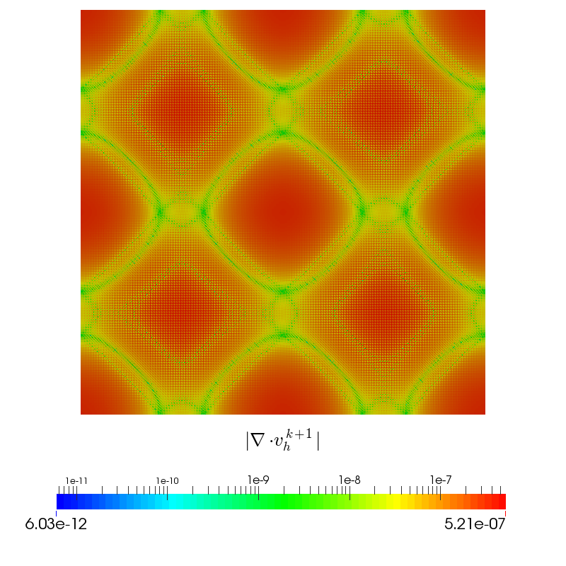
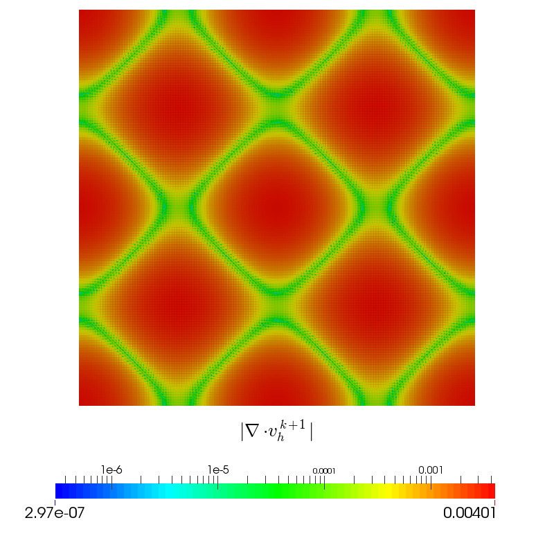
Figure 1: Pointwise divergence of the Taylor-Green vortex solution at time 1 with $\Delta t=0.025$ obtained by the RIPCS.
Left part shows $\mathcal{Q}_{2}/\mathcal{Q}_{1}$ with div-div projection. Right part shows $\mathcal{Q}_{2}/\mathcal{Q}_{1}$ with reconstruction in $\textup{RT}_{h}^{0}$.

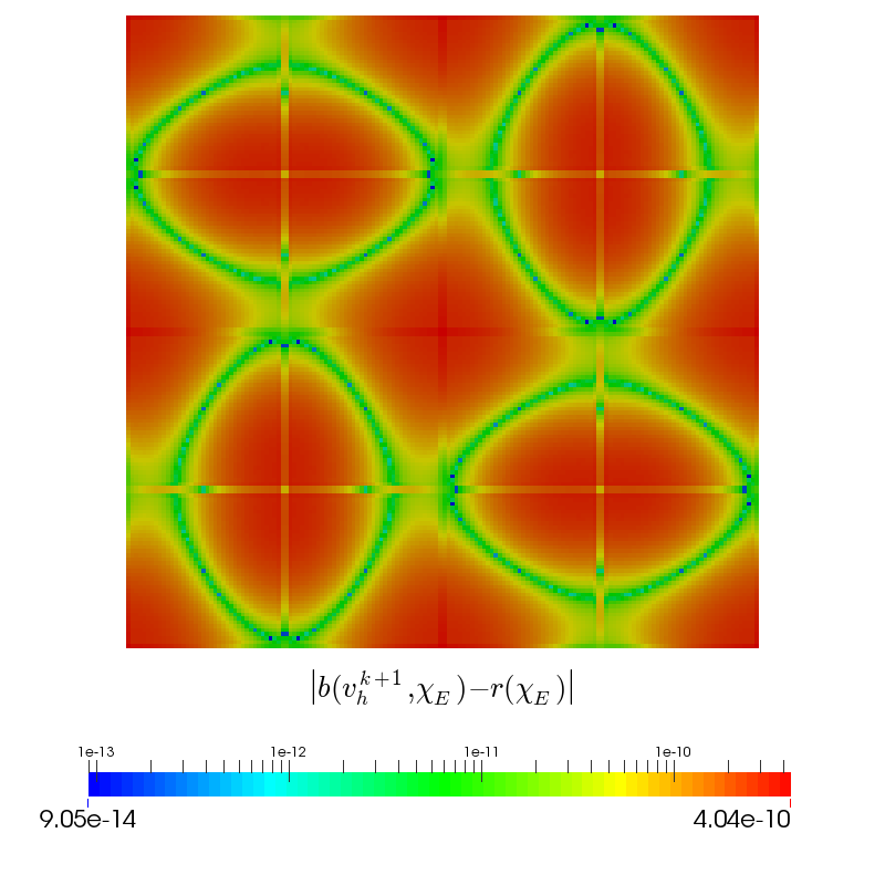
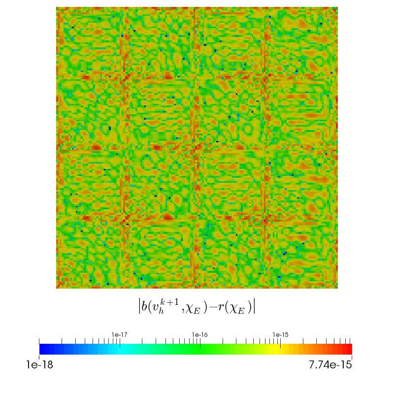
Figure 2: Local mass conservation of the Taylor-Green vortex solution at time 1 with $\Delta t=0.025$ obtained by the RIPCS.
Left part shows $\mathcal{Q}_{2}/\mathcal{Q}_{1}$ with div-div projection. Right part shows $\mathcal{Q}_{2}/\mathcal{Q}_{1}$ with reconstruction $\textup{RT}_{h}^{0}$, identical to reconstruction in $\textup{RT}_{h}^{1}$.

4.3 Global Dirichlet boundary conditions

We consider the Stokes equations on the domain $\Omega=(0,1)^{2}$ and take the exact solution to be

$$v_{1}(x,y,t) =\sin\left(x+t\right)\,\sin\left(y+t\right)$$

$$v_{2}(x,y,t) =\cos\left(x+t\right)\,\cos\left(y+t\right)$$

$$p(x,y,t) =\sin\left(x-y+t\right)\;.$$ (40)

The source term is given by $f=\partial_{t}v-\Delta v+\nabla p$. The density and viscosity are both set to $\rho=\mu=1$. Computations were done on a $160\times 160$ rectangular mesh.

Figure 3 shows the error and the convergence rates as function of $\Delta t$ for the IPCS and RIPCS. The green curves show the $L^{2}$-error for the velocity, the red curves the $H_{0}^{1}$-error for the velocity and the blue curves the $L^{2}$-error for the pressure obtained by the polynomial degrees $p=2,3,4$. The curves grouped by the same color are almost identical meaning that the splitting error is dominant in the measured range of $\Delta t$. Therefore we have left out the curves with $p=4$ on the right for the sake of clarity. A transition towards smaller time steps causes earlier flattening out of the error curves the lower the spatial order is. This emerges at first for the $H_{0}^{1}$-error for the velocity and $L^{2}$-error for the pressure. This is demonstrated for the Taylor-Green vortex solution in section 4.5, c.f. right of figure 5.

Theory states that the solution of the second order IPCS satisfies the following error estimates: (I) $L^{2}$-velocity: $\mathcal{O}(\Delta t^{2})$ (II) $H_{0}^{1}$-velocity, $L^{2}$-pressure: $\mathcal{O}(\Delta t)$. On the left of figure 3 it is observed that the velocity error in the $L^{2}$-norm is second order accurate, in the other two error measures the rate is 1.5 which is better than the prediction. Now the solution of the RIPCS satisfies the following error estimates: (I) $L^{2}$-velocity: $\mathcal{O}(\Delta t^{2})$ (II) $H_{0}^{1}$-velocity, $L^{2}$-pressure: $\mathcal{O}(\Delta t^{\frac{3}{2}})$. The convergence rates on the right of figure 3 are consistent with the error estimates. Note that the $L^{2}$-errors on the velocity and pressure are almost identical to the results presented in [16]. The reason for the slight difference is likely to be the usage of BDF2 in [16] as time stepping.

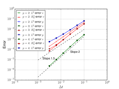
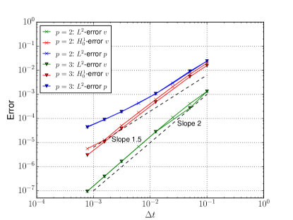
Figure 3: Errors and convergence rates at final time T=1 for the global Dirichlet problem and spatial discretizations $\mathcal{Q}_{2}/\mathcal{Q}_{1}$, $\mathcal{Q}_{3}/\mathcal{Q}_{2}$, $\mathcal{Q}_{4}/\mathcal{Q}_{3}$. Left part shows the IPCS. Right part shows the RIPCS.

A consideration of local mass conservation shows that it is well satisfied in the interior of the domain for the div-div projection. However the largest values $\sim 10^{-9}$ are located in the cells that share an edge with the boundary. This is due to the artificial boundary conditions on the pressure.

The situation is different for the $H(\text{div})$ reconstruction. In that case the distribution is similar to the right in figure 2 with $\max_{E}|b(v_{h}^{k+1},\chi_{E})-r(\chi_{E})|\sim 5\cdot 10^{-14}$.

4.4 Mixed boundary conditions

We consider again the Stokes equations on the domain $\Omega=(0,1)^{2}$ and take the exact solution to be

$$v_{1}(x,y,t) =\sin x\,\sin\left(y+t\right)$$

$$v_{2}(x,y,t) =\cos x\,\cos\left(y+t\right)$$

$$p(x,y,t) =\cos x\,\sin\left(y+t\right)\;.$$ (41)

The source term is again given by $f=\partial_{t}v-\Delta v+\nabla p$. The density and viscosity are both set to $\rho=\mu=1$. The outflow boundary is located at $\Gamma_{N}=\{(x,y)\in\partial\Omega\mid x=0\}$. Computations were done on $160\times 160$ rectangular mesh.

Figure 4 shows the error and the convergence rates as function of $\Delta t$ for the IPCS and RIPCS. The green curves show the $L^{2}$-error for the velocity, the red curves the $H_{0}^{1}$-error for the velocity and the blue curves the $L^{2}$-error for the pressure obtained by the polynomial degrees $p=2,3,4$. The curves grouped by the same color are almost identical meaning that the splitting error is dominant in the measured range of $\Delta t$. Therefore we have left out the curves with $p=3$ on the left and $p=4$ on the right for the sake of clarity. A transition towards smaller time steps causes earlier flattening out of the error curves the lower the spatial order is. This emerges at first for the $H_{0}^{1}$-error for the velocity and $L^{2}$-error for the pressure. This is demonstrated for the Taylor-Green vortex solution in section 4.5, c.f. right of figure 5.

The solution of the IPCS satisfies the following error estimates: (I) $L^{2}$-velocity: $\mathcal{O}(\Delta t)$ (II) $H_{0}^{1}$-velocity, $L^{2}$-pressure: $\mathcal{O}(\Delta t^{\frac{1}{2}})$ which are identical to the first order IPCS. The results on the left of figure 4 indeed show that the pressure approximation is poor due to the homogeneous Dirichlet boundary condition imposed on $\Gamma_{N}$. The RIPCS delivers improved error estimates in presence of mixed boundary conditions: (I) $L^{2}$-velocity: $\mathcal{O}(\Delta t^{\frac{3}{2}})$ (II) $H_{0}^{1}$-velocity, $L^{2}$-pressure: $\mathcal{O}(\Delta t)$. The convergence rates on right of figure 4 are consistent with those estimates. Furthermore the error on the velocity in the $L^{2}$-norm behaves like $\mathcal{O}(\Delta t^{\frac{5}{3}})$ which is also observed in Guermond, Minev and Shen [18, 24]. The error in the $H_{0}^{1}$-norm is close to $\mathcal{O}(\Delta t^{\frac{5}{4}})$ which is higher than the rate $\mathcal{O}(\Delta t)$ predicted by theory. Note that [18, 24] have used BDF2 as time stepping for this problem and therefore the error curves are almost identical.

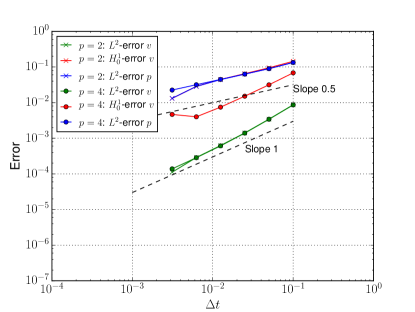
Figure 4: Errors and convergence rates at final time T=1 for the mixed boundary condition problem and spatial discretizations $\mathcal{Q}_{2}/\mathcal{Q}_{1}$, $\mathcal{Q}_{3}/\mathcal{Q}_{2}$, $\mathcal{Q}_{4}/\mathcal{Q}_{3}$. Left part shows the IPCS. Right part shows the RIPCS.

Another consideration of local mass conservation shows that it is well satisfied in the interior of the domain. But due to the homogeneous Dirichlet boundary conditions for the pressure imposed on $\Gamma_{N}$, the largest errors $\sim 10^{-7}$ are located in the cells next to outflow boundary.

With the $H(\text{div})$ reconstruction we have $\max_{E}|b(v_{h}^{k+1},\chi_{E})-r(\chi_{E})|\sim 5\cdot 10^{-14}$ whereat the maximum also occurs in the boundary cells.

4.5 Periodic boundary conditions

We continue with the configuration and test problem presented in 4.2. Figure 5 shows the error and convergence rates as a function of $\Delta t$ for the IPCS and RIPCS. The green curves show the $L^{2}$-error for the velocity, the red curves the $H_{0}^{1}$-error for the velocity and the blue curves the $L^{2}$-error for the pressure obtained by the polynomial degrees $p=2,3$. The results for $p=4$ are almost identical to $p=3$, therefore it has been omitted for the sake of clarity. For the IPCS the curves grouped by the same color are almost identical meaning that the splitting error is dominant in the measured range of $\Delta t$. Note however that for $p=2$ in the RIPCS the spatial error is already not negligible in this range and becomes all-dominant for additionally smaller time steps taken. It can be seen on the right that the $H_{0}^{1}$-error on the velocity and $L^{2}$-error on the pressure flattens out whereas the errors from spatial order three continue decreasing with the same rate. That puts in favour higher polynomial degrees since the error on the same spatial mesh for moderate time step sizes is minimized.

There is no rigorous error analysis of the projection methods for purely periodic boundary conditions. But since in the periodic case no artificial boundary conditions are imposed on the pressure, both the standard and rotational formulation are expected to be fully second order accurate. This is validated for the pressure-correction schemes in figure 5. The error of the RIPCS is slightly lower than the error of the IPCS, but both schemes have the same convergence rate. It is close to $\mathcal{O}(\Delta t^{2})$ in the $L^{2}$-norm on the pressure while the rates of the velocity in the $L^{2}$-norm and $H_{0}^{1}$-norm are perfectly of second order.

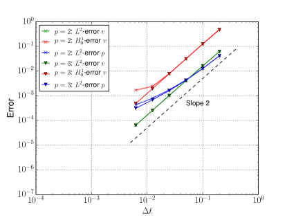
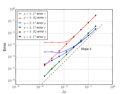
Figure 5: Errors and convergence rates at final time T=2 for the periodic boundary condition problem and spatial discretizations $\mathcal{Q}_{2}/\mathcal{Q}_{1}$, $\mathcal{Q}_{3}/\mathcal{Q}_{2}$, $\mathcal{Q}_{4}/\mathcal{Q}_{3}$. Left part shows the IPCS. Right part shows the RIPCS.

The absence of artificial boundary conditions also implies that the error on local mass conservation is distributed over the interior on the domain. This was shown before in figure 2.

4.6 Beltrami flow

The Beltrami flow is one of the rare test problems where an exact fully three-dimensional solution of the Navier-Stokes equations is derived. It has its origin from [42] and has been later studied by [43]. The domain is $\Omega=(-1,1)^{3}$ and global Dirichlet boundary conditions are imposed by the exact solution

$$\begin{split}v_{1}(x,y,z,t)&=-a\,e^{-d^{2}\,t}\,\left(e^{a\,x}\,\sin\left(d\,z+a\,y\right)+\cos\left(d\,y+a\,x\right)\,e^{a\,z}\right)\\ v_{2}(x,y,z,t)&=-a\,e^{-d^{2}\,t}\,\left(e^{a\,x}\,\cos\left(d\,z+a\,y\right)+e^{a\,y}\,\sin\left(a\,z+d\,x\right)\right)\\ v_{3}(x,y,z,t)&=-a\,e^{-d^{2}\,t}\,\left(e^{a\,y}\,\cos\left(a\,z+d\,x\right)+\sin\left(d\,y+a\,x\right)\,e^{a\,z}\right)\\ p(x,y,z,t)&=-0.5\,a^{2}\,\rho\,e^{-d^{2}\,t}\,(2\,\cos\left(d\,y+a\,x\right)\,e^{a\,\left(z+x\right)}\,\sin\left(d\,z+a\,y\right)\\ &\quad+2\,e^{a\,\left(y+x\right)}\,\sin\left(a\,z+d\,x\right)\,\cos\left(d\,z+a\,y\right)\\ &\quad+2\,\sin\left(d\,y+a\,x\right)\,e^{a\,\left(z+y\right)}\,\cos\left(a\,z+d\,x\right)+e^{2\,a\,z}+e^{2\,a\,y}+e^{2\,a\,x})\;.\end{split}$$ (42)

The Beltrami flow has the property that the velocity and vorticity vectors are aligned, namely $d\;v-\nabla\times v=0$ The source term is given by $f=0$, the density, viscosity are set to $\rho=\mu=1$. The constants $a$ and $d$ may be chosen arbitrarily and have been set to $a=\pi/4$, $d=\pi/2$ as in [42]. Computations were done on a $50\times 50\times 50$ cubic mesh.

Figure 6 shows the error and convergence rates as a function of $\Delta t$ for the RIPCS. The green curves show the $L^{2}$-error for the velocity and the red curves the $H_{0}^{1}$-error for the velocity obtained by the polynomial degrees $p=2,3$. The curves grouped by the same color are almost identical meaning that the splitting error is dominant in the measured range of $\Delta t$. It can be concluded from the figure that error is fully second order convergent in both norms.

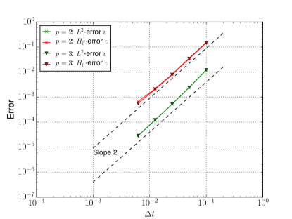
Figure 6: Errors and convergence rates at final time T=0.5 for the Beltrami test problem using the RIPCS with the spatial discretizations $\mathcal{Q}_{2}/\mathcal{Q}_{1}$, $\mathcal{Q}_{3}/\mathcal{Q}_{2}$.

4.7 3D DNS of turbulent flows

We test the applicability of the code to direct numerical simulations (DNS) with two examples.

4.7.1 3D Driven Cavity

The driven cavity flow is a commonly used benchmark problem due to its simple geometry. We take the configuration based on [44]. We shift the domain to $\Omega=(0,1)^{3}$ instead, set $\rho=1$ and $\textup{Re}=1/\mu=10000$. The driving velocity at $y=1$ has a continuous ramp profile in time given by $v=(\min(t,1),0,0)^{T}$. The simulation is computed on a $50\times 50\times 50$ grid using the $\mathcal{Q}_{3}/\mathcal{Q}_{2}$ discretization with reconstruction in $\textup{RT}_{h}^{1}$. The temporal interval starts from $t_{0}=0$ up to 50, Alexander’s second order strongly S-stable scheme is used with time step size $\Delta t=0.005$.

The flow transitions to a chaotic behaviour at $t\sim 12$. Figure 7 shows two snapshots of the flow in the driven cavity. The left part of the figure shows $\left\|v\right\|_{2}$ together with streamlines of $v_{\parallel}$ on the plane $x=0.5$. The characteristic corner vortices on this cut through the domain are clearly visible as well as the appearance of the Taylor-Görtler vortices close to $z=0.5$. The right part of the figure shows the z-component of the vorticity $\nabla\times v$ on the plane $z=0.5$ after the main initial vortex has decayed into several small eddies.

The figure demonstrates in general long time stability of the spatial discretization $\mathcal{Q}_{3}/\mathcal{Q}_{2}$ and reconstruction in $\textup{RT}_{h}^{1}$ with $10^{4}$ time steps taken.

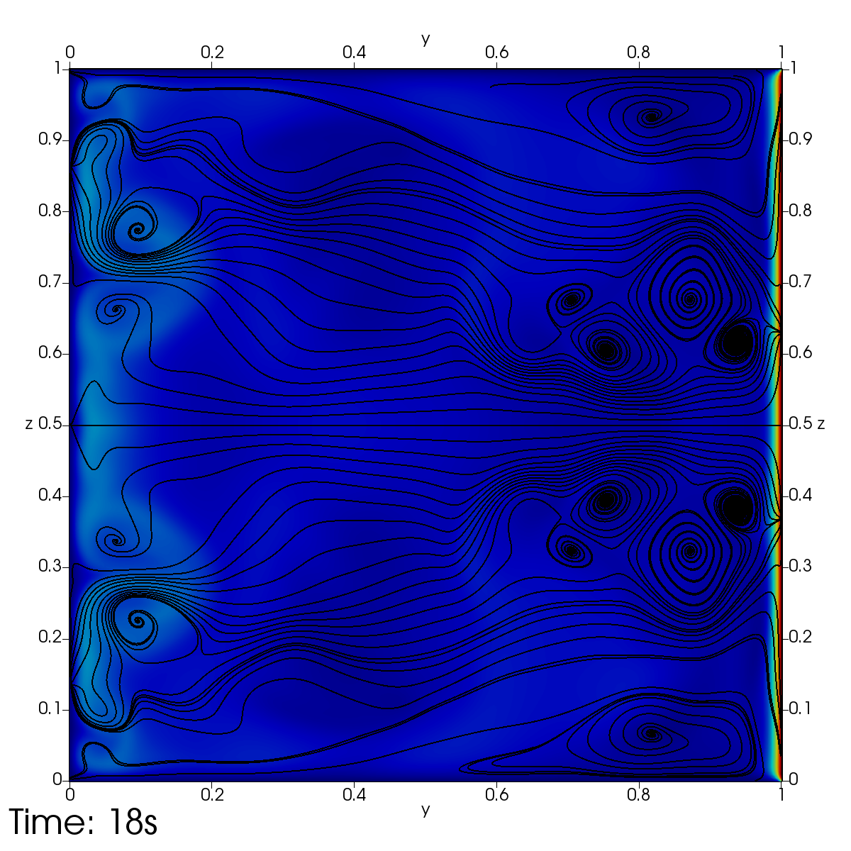
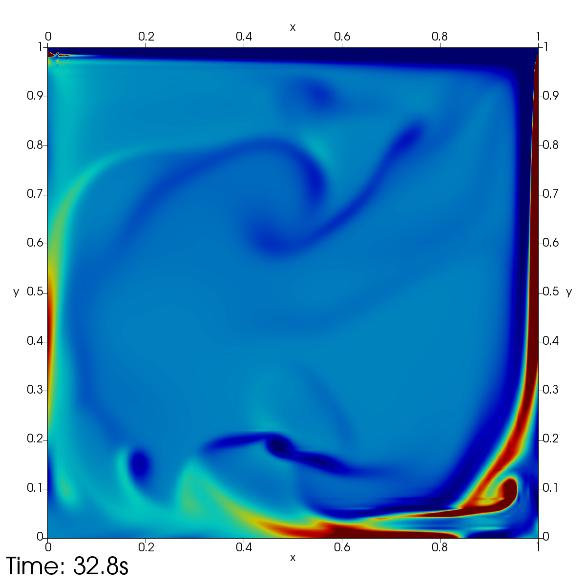
Figure 7: Time-snapshot of $\left\|v\right\|_{2}$ and streamlines of $v_{\parallel}$ on plane $x=0.5$ (left). Time-snapshot of z-component of the vorticity $\nabla\times v$ on plane $z=0.5$ (right).

4.7.2 3D Taylor-Green vortex

The Taylor-Green vortex has been studied in great detail in [45], C3.5. It aims at testing the accuracy and the performance of high-order methods in the DNS. The initial flow field is given by

$$v_{1}(x,y,z,t) =V_{0}\sin\left(\frac{x}{L}\right)\cos\left(\frac{y}{L}\right)\cos\left(\frac{z}{L}\right)$$

$$v_{2}(x,y,z,t) =-V_{0}\cos\left(\frac{x}{L}\right)\sin\left(\frac{y}{L}\right)\cos\left(\frac{z}{L}\right)$$

$$v_{3}(x,y,z,t) =0$$

$$p(x,y,z,t) =p_{0}+\frac{\rho_{0}V_{0}^{2}}{16}\left(\cos\left(\frac{2x}{L}\right)+\cos\left(\frac{2y}{L}\right)\right)\left(\cos\left(\frac{2z}{L}\right)+2\right)$$ (43)

with periodic boundary conditions in all directions. The general extension of the domain is $\Omega=(-\pi L,\pi L)^{3}$ and the Reynolds number is given by $\textup{Re}=\frac{\rho_{0}V_{0}L}{\mu}$. As in the references [43, 45] we set $L=1,\;V_{0}=1,\;\rho_{0}=1,\;p_{0}=0,\;\textup{Re}=1600$. In three dimensions the flow transitions to turbulence with development of small scale structures. The simulation is computed on a $105\times 105\times 105$ grid using the $\mathcal{Q}_{3}/\mathcal{Q}_{2}$ discretization with reconstruction in $\textup{RT}_{h}^{1}$ which leads to about $2\cdot 10^{8}$ degrees of freedom. The temporal interval starts from $t_{0}=0$ up to 20, Alexander’s second order strongly S-stable scheme is used with time step size $\Delta t=0.005$.

Figure 8 shows the contour surfaces of the z-component of the vorticity for the values 0.5 in red and -0.5 in blue, respectively, at initial and final condition.

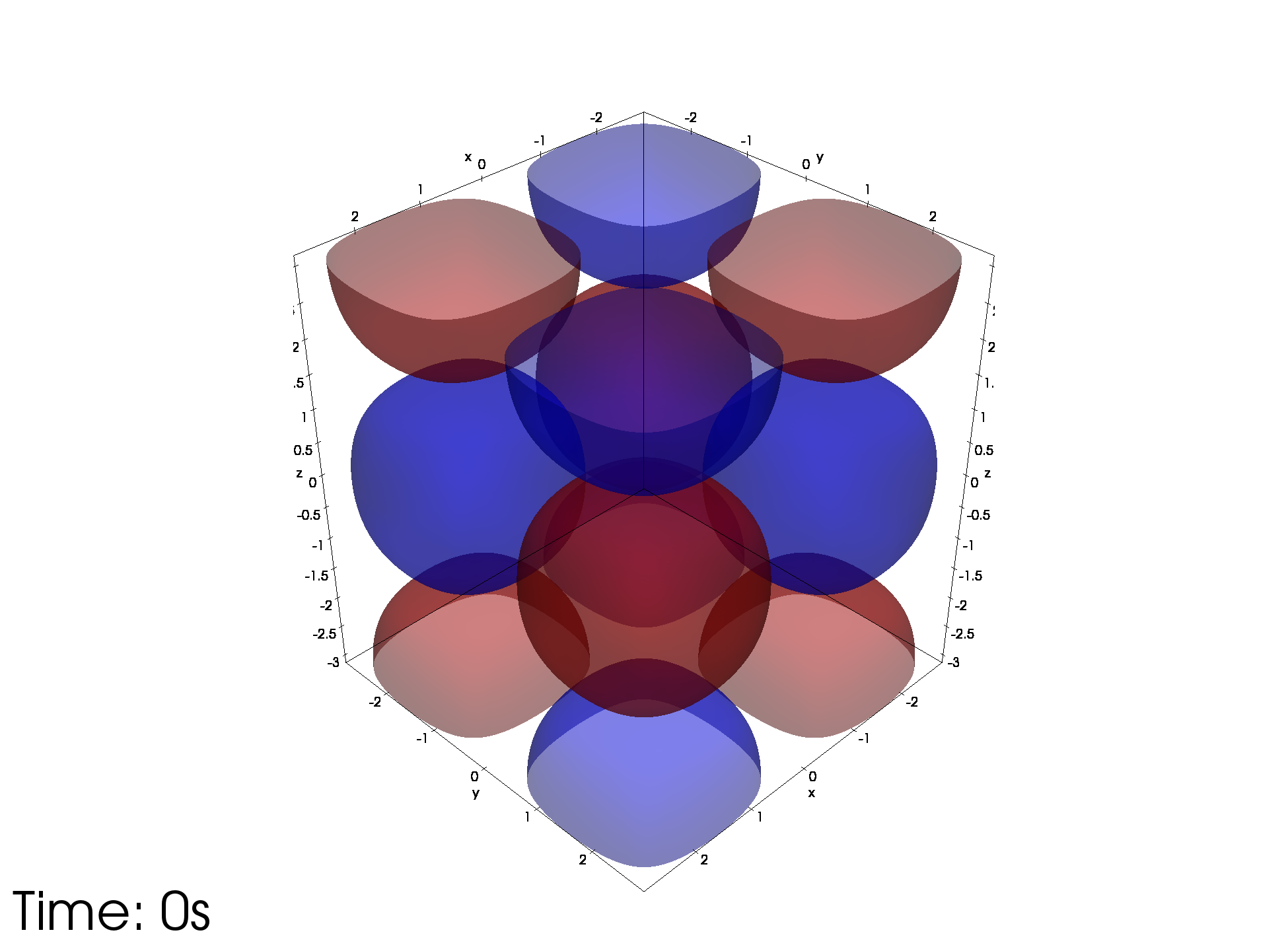
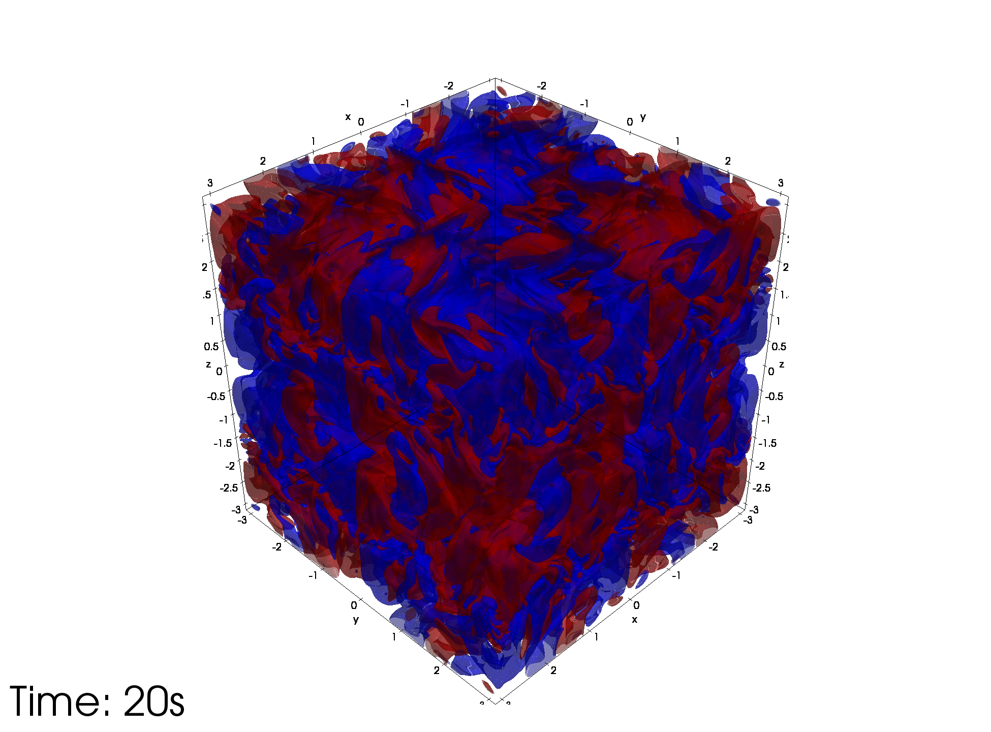
Figure 8: Vorticity visualization for the Taylor-Green vortex problem. The red contours show the levels of the vorticity z-component with 25 percent of the instantaneous peak. The blue contours show the corresponding negative level.

We now compare our results to the reference values given for this problem that contain the temporal evolution of

• the kinetic energy, $E_{k}=\frac{1}{\rho\left|\Omega\right|}\frac{1}{2}(v,v)_{0,\Omega}$,

• the dissipation rate, $\epsilon=\frac{\nu}{\left|\Omega\right|}(\nabla v,\nabla v)_{0,\Omega}$,

• the enstrophy, $\qquad\;\mathcal{E}=\frac{1}{\rho\left|\Omega\right|}\frac{1}{2}(\nabla\times v,\nabla\times v)_{0,\Omega}\;.$

The reference solution was obtained with a dealiased pseudo-spectral code run on a $512^{3}$ grid, time integration was performed with a low-storage three-step Runge-Kutta scheme and a time step of $\Delta t=10^{-3}$. The comparison of these three reference quantities is presented in figure 9. Our enstrophy curve is extremely close to the reference curve, furthermore the curves for the kinetic energy and the dissipation rate are indistinguishable with respect to the reference curves.

It can be concluded that the spatial discretization $\mathcal{Q}_{3}/\mathcal{Q}_{2}$ and reconstruction in $\textup{RT}_{h}^{1}$ together with the upwind scheme based on the Vijayasundaram flux exhibits long time stability - as in the three-dimensional driven cavity problem - and is good at capturing turbulence accurately.

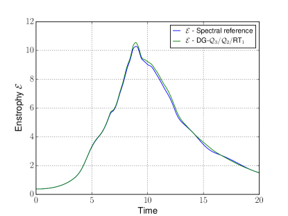
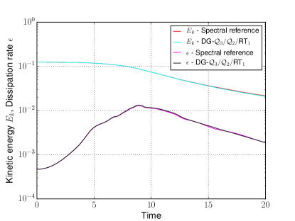
Figure 9: Evolution of the kinetic energy, dissipation rate and enstrophy for the $\mathcal{Q}_{3}/\mathcal{Q}_{2}$ discretization with reconstruction in $\textup{RT}_{h}^{1}$ and comparison with the reference values from the spectral code.

5 Conclusion and Outlook

In this paper we considered splitting methods, in particular the incremental and rotational incremental pressure correction schemes in combination with a high-order discontinuous Galerkin discretization in space. The momentum equation is solved fully-implicitly with a matrix-free Newton method and sum-factorized element computations to achieve reduced computational complexity at high floating-point performance. The upwind discretization of the convective term in the momentum equation uses a modified Vijayasundaram numerical flux function that takes into account that the discrete velocity field is not in $H(\text{div})$. In the Helmholtz projection step we employ an $H(\text{div})$ postprocessing of the velocity correction which ensures that the projected velocity satisfies the discrete continuity equation. Numerical results confirm that RIPCS is second-order convergent in time for Dirichlet and periodic boundary conditions and has convergence order 1.5 for mixed boundary conditions. Three-dimensional computations with up to $2\cdot 10^{8}$ degrees of freedom and about $10^{4}$ time steps show that the scheme is stable for long time computations.

The $H(\text{div})$ postprocessing in $RT_{k}$ spaces is restricted to parallelepiped elements due to the Piola transformation. It remains an open problem how to extend the postprocessing scheme to more general element transformations. In a forthcoming publication we will focus on the performance characteristics and scalability of the parallel implementation.

References

-
[1]
B. Rivière, V. Girault,
Discontinuous
finite element methods for incompressible flows on subdomains with
non-matching interfaces, Computer Methods in Applied Mechanics and
Engineering 195 (25–28) (2006) 3274 – 3292, discontinuous Galerkin
Methods.
doi:http://dx.doi.org/10.1016/j.cma.2005.06.014.
URL http://www.sciencedirect.com/science/article/pii/S0045782505002690 - [2] V. Girault, B. Rivière, Mary, F. Wheeler, A discontinuous galerkin method with nonoverlapping domain decomposition for the stokes and navier-stokes problems, Math. Comp (2004) 53–84.
-
[3]
E. Ferrer, R. Willden,
A
high order discontinuous galerkin finite element solver for the
incompressible navier–stokes equations, Computers & Fluids 46 (1) (2011)
224 – 230, 10th {ICFD} Conference Series on Numerical Methods for Fluid
Dynamics (ICFD 2010).
doi:http://dx.doi.org/10.1016/j.compfluid.2010.10.018.
URL http://www.sciencedirect.com/science/article/pii/S0045793010002860 - [4] B. Krank, N. Fehn, W. A. Wall, M. Kronbichler, A high-order semi-explicit discontinuous Galerkin solver for 3D incompressible flow with application to DNS and LES of turbulent channel flow, ArXiv e-printsarXiv:1607.01323.
- [5] S. Müthing, M. Piatkowski, P. Bastian, High-performance implementation of matrix-free spectral discontinuous galerkin methods, In preparation.
-
[6]
E. J. Dean, R. Glowinski,
On some finite element
methods for the numerical simulation of incompressible viscous flow, in:
M. D. Gunzburger, R. A. Nicolaides (Eds.), Incompressible Computational Fluid
Dynamics, Cambridge University Press, 1993, pp. 17–66, cambridge Books
Online.
URL http://dx.doi.org/10.1017/CBO9780511574856.003 - [7] H. C. Elman, D. J. Silvester, A. J. Wathen, Finite elements and fast iterative solvers: with applications in incompressible fluid dynamics, Oxford University Press, 2014, second edition.
-
[8]
A. J. Chorin, Numerical solution of
the navier-stokes equations, Mathematics of Computation 22 (104) (1968)
745–762.
URL http://www.jstor.org/stable/2004575 -
[9]
R. Témam, Sur l’approximation de
la solution des équations de navier-stokes par la méthode des pas
fractionnaires (ii), Archive for Rational Mechanics and Analysis 33 (5)
(1969) 377–385.
doi:10.1007/BF00247696.
URL http://dx.doi.org/10.1007/BF00247696 -
[10]
R. Rannacher, On chorin’s
projection method for the incompressible navier-stokes equations, Springer
Berlin Heidelberg, Berlin, Heidelberg, 1992, pp. 167–183.
doi:10.1007/BFb0090341.
URL http://dx.doi.org/10.1007/BFb0090341 - [11] W. E, J.-G. Liu, Projection method i: Convergence and numerical boundary layers, SIAM Journal on Numerical Analysis 32 (4) (1995) 1017–1057. doi:10.1137/0732047.
- [12] W. E, J.-G. Liu, Projection method ii: Godunov–ryabenki analysis, SIAM Journal on Numerical Analysis 33 (4) (1996) 1597–1621. doi:10.1137/S003614299426450X.
-
[13]
G. E. Karniadakis, M. Israeli, S. A. Orszag,
High-order
splitting methods for the incompressible navier-stokes equations, Journal of
Computational Physics 97 (2) (1991) 414 – 443.
doi:http://dx.doi.org/10.1016/0021-9991(91)90007-8.
URL http://www.sciencedirect.com/science/article/pii/0021999191900078 - [14] L. J. P. Timmermans, P. D. Minev, F. N. Van De Vosse, An approximate projection scheme for incompressible flow using spectral elements, International Journal for Numerical Methods in Fluids 22 (7) (1996) 673–688.
- [15] J. L. Guermond, J. Shen, A new class of truly consistent splitting schemes for incompressible flows, J. Comput. Phys. 192 (2003) 262–276.
- [16] J. L. Guermond, J. Shen, On the error estimates of rotational pressure-correction projection methods, Math. Comp 73 (2004) 1719–1737.
- [17] G. Karniadakis, S. Sherwin, Spectral/hp Element Methods for Computational Fluid Dynamics, Oxford University Press, 2005.
- [18] J. L. Guermond, P. Minev, J. Shen, An overview of projection methods for incompressible flows, Computer Methods in Applied Mechanics and Engineering 195 (2006) 6011–6045.
-
[19]
K. Goda,
A
multistep technique with implicit difference schemes for calculating two- or
three-dimensional cavity flows, Journal of Computational Physics 30 (1)
(1979) 76 – 95.
doi:http://dx.doi.org/10.1016/0021-9991(79)90088-3.
URL http://www.sciencedirect.com/science/article/pii/0021999179900883 -
[20]
D. Steinmoeller, M. Stastna, K. Lamb,
A
short note on the discontinuous galerkin discretization of the pressure
projection operator in incompressible flow, Journal of Computational Physics
251 (2013) 480 – 486.
doi:http://dx.doi.org/10.1016/j.jcp.2013.05.036.
URL http://www.sciencedirect.com/science/article/pii/S0021999113004026 -
[21]
S. M. Joshi, P. J. Diamessis, D. T. Steinmoeller, M. Stastna, G. N. Thomsen,
A
post-processing technique for stabilizing the discontinuous pressure
projection operator in marginally-resolved incompressible inviscid flow,
Computers & Fluids 139 (2016) 120 – 129, 13th {USNCCM} International
Symposium of High-Order Methods for Computational Fluid Dynamics - A special
issue dedicated to the 60th birthday of Professor David Kopriva.
doi:http://dx.doi.org/10.1016/j.compfluid.2016.04.021.
URL http://www.sciencedirect.com/science/article/pii/S0045793016301311 -
[22]
P. Bastian, B. Rivière,
Superconvergence and h(div)
projection for discontinuous galerkin methods, International Journal for
Numerical Methods in Fluids 42 (10) (2003) 1043–1057.
doi:10.1002/fld.562.
URL http://dx.doi.org/10.1002/fld.562 -
[23]
A. Ern, S. Nicaise, M. Vohralík,
An
accurate H(div) flux reconstruction for discontinuous Galerkin
approximations of elliptic problems, Comptes Rendus Mathematique 345 (12)
(2007) 709 – 712.
doi:http://dx.doi.org/10.1016/j.crma.2007.10.036.
URL http://www.sciencedirect.com/science/article/pii/S1631073X07004360 -
[24]
J. L. Guermond, P. Minev, J. Shen,
Error analysis of
pressure-correction schemes for the time-dependent stokes equations with open
boundary conditions, SIAM Journal on Numerical Analysis 43 (1) (2005)
239–258.
arXiv:http://dx.doi.org/10.1137/040604418, doi:10.1137/040604418.
URL http://dx.doi.org/10.1137/040604418 - [25] V. Girault, P. Raviart, Finite Element Methods for the Navier-Stokes Equations, Springer, 1986.
- [26] R. Témam, Navier-Stokes Equations. Theory and numerical analysis, North Holland, Amsterdam, 1987.
- [27] P. Houston, R. Hartmann, An optimal order interior penalty discontinuous Galerkin discretization of the compressible Navier-Stokes equations, J. Comp. Phys. 227 (2008) 9670–9685.
- [28] P. Bastian, M. Blatt, R. Scheichl, Algebraic multigrid for discontinuous Galerkin discretizations, Numer. Linear Algebra Appl. 19 (2) (2012) 367–388. doi:10.1002/nla.1816.
- [29] M. Feistauer, J. Felcman, I. Straskraba, Mathematical and Computational Methods for Compressible Flow, Clarendon Press, 2003.
-
[30]
V. Dolejší, M. Feistauer,
A
semi-implicit discontinuous galerkin finite element method for the numerical
solution of inviscid compressible flow, Journal of Computational Physics
198 (2) (2004) 727 – 746.
doi:http://dx.doi.org/10.1016/j.jcp.2004.01.023.
URL http://www.sciencedirect.com/science/article/pii/S0021999104000609 - [31] L. Evans, Partial Differential Equations, 2nd Edition, American Mathematical Society, 2010.
- [32] J.-L. G. a. Alexandre Ern, Theory and Practice of Finite Elements, 1st Edition, Applied Mathematical Sciences 159, Springer-Verlag New York, 2004.
- [33] B. Schweizer, Partielle Differentialgleichungen, Eine anwendungsorientierte Einführung, Springer-Verlag, 2013.
-
[34]
H. Bhatia, G. Norgard, V. Pascucci, P.-T. Bremer,
The helmholtz-hodge
decomposition—a survey, IEEE Transactions on Visualization and
Computer Graphics 19 (8) (2013) 1386–1404.
doi:10.1109/TVCG.2012.316.
URL http://dx.doi.org/10.1109/TVCG.2012.316 - [35] F. Brezzi, M. Fortin, Mixed and Hybrid Finite Element Methods, Springer-Verlag, 1991.
- [36] R. Alexander, Diagonally implicit Runge–Kutta methods for stiff O.D.E.’s, SIAM Journal on Numerical Analysis 14 (6) (1977) 1006–1021.
- [37] P. Bastian, M. Blatt, A. Dedner, C. Engwer, R. Klöfkorn, M. Ohlberger, O. Sander, A generic grid interface for parallel and adaptive scientific computing. Part I: Abstract framework, Computing 82 (2–3) (2008) 103–119. doi:10.1007/s00607-008-0003-x.
-
[38]
P. Bastian, C. Engwer, J. Fahlke, M. Geveler, D. Göddeke, O. Iliev,
O. Ippisch, R. Milk, J. Mohring, S. Müthing, M. Ohlberger, D. Ribbrock,
S. Turek,
Hardware-Based
Efficiency Advances in the EXA-DUNE Project, Springer International
Publishing, Cham, 2016, p. 3–23.
doi:10.1007/978-3-319-40528-5_1.
URL http://dx.doi.org/10.1007/978-3-319-40528-5_1 - [39] M. Kronbichler, K. Kormann, A generic interface for parallel cell-based finite element operator application, Computers & Fluids 63 (2012) 135–147.
-
[40]
G. I. Taylor, A. E. Green, Mechanism
of the production of small eddies from large ones, Proceedings of the Royal
Society of London. Series A, Mathematical and Physical Sciences 158 (895)
(1937) 499–521.
URL http://www.jstor.org/stable/96892 - [41] P. Rabenold, E. Balaras, Parallel adaptive mesh refinement for the incompressible navier-stokes equations.
- [42] C. R. Ethier, D. A. Steinmann, Exact fully 3D Navier–Stokes solution for benchmarking, Internat. J. Numer. Methods Fluids 19 (1994) 369 – 375.
-
[43]
A. Logg, K.-A. Mardal, G. N. Wells (Eds.),
Automated Solution of
Differential Equations by the Finite Element Method, Vol. 84 of Lecture
Notes in Computational Science and Engineering, Springer, 2012.
doi:10.1007/978-3-642-23099-8.
URL http://dx.doi.org/10.1007/978-3-642-23099-8 -
[44]
R. Iwatsu, K. Ishii, T. Kawamura, K. Kuwahara, J. M. Hyun,
Numerical simulation of
three-dimensional flow structure in a driven cavity, Fluid Dynamics
Research 5 (3) (1989) 173.
URL http://stacks.iop.org/1873-7005/5/i=3/a=A03 -
[45]
2nd international workshop on high-order cfd
methods, cologne, germany (May 2013).
URL http://www.dlr.de/as/hiocfd