Spontaneous symmetry breaking induced by complex fermion determinant — yet another success of the complex Langevin method

Abstract:

In many interesting systems, the fermion determinant becomes complex and its phase plays a crucial role in the determination of the vacuum. For instance, in finite density QCD at low temperature and high density, exotic fermion condensates are conjectured to form due to such effects. When one applies the complex Langevin method to such a complex action system naively, one cannot obtain the correct results because of the singular-drift problem associated with the appearance of small eigenvalues of the Dirac operator. Here we propose to avoid this problem by adding a fermion bilinear term to the action and extrapolating its coefficient to zero. We test this idea in an SO(4)-invariant matrix model with a Gaussian action and a complex fermion determinant, whose phase is expected to induce the spontaneous breaking of the SO(4) symmetry. Our results agree well with the previous results obtained by the Gaussian expansion method.

1 Introduction

Monte Carlo methods are difficult to apply to a system with a complex action $S$ because of a notorious technical problem known as the sign problem. The importance sampling cannot be applied since the integrand $\exp\left(-S\right)$ of the partition function cannot be regarded as the probability distribution. The complex Langevin method (CLM) [1, 2] is a promising approach to such complex-action systems. It may be regarded as an extension of the stochastic quantization based on the Langevin equation, where the dynamical variables of the original system are complexified and the observables as well as the drift term are extended holomorphically by analytic continuation.

An important remaining problem of the CLM is that the method gives wrong results when the determinant that appears from integrating out fermions takes values close to zero during the complex Langevin simulation [3]. A theoretical understanding of this problem has been given recently [4], where it was recognized that the probability distribution of the complexified variables has to fall off fast enough near the singularities of the drift term in order to justify the CLM along the line of the argument [5]. See also ref. [6] for the proposal of a new criterion for justification based on a refined argument.

In many systems with a complex fermion determinant, its phase is expected to play a crucial role in the determination of the vacuum. For instance, in finite density QCD at low temperature and high density, the phase is conjectured to induce the formation of various exotic fermion condensates. Also in the Euclidean version of the type IIB matrix model [7] for 10d superstring theory, the phase is conjectured to induce the SSB of the SO(10) rotational symmetry.

When one applies the CLM to these systems, the singular-drift problem occurs because of the appearance of eigenvalues of the Dirac operator close to zero. Here we propose to avoid this problem by deforming the action with a fermion bilinear term and extrapolating its coefficient to zero. The fermion bilinear term has to be chosen carefully in such a way that the nearly zero eigenvalues of the Dirac operator are avoided and yet the vacuum of the system is minimally affected.

We test this idea in an SO(4)-symmetric matrix model with a Gaussian action and a complex fermion determinant, in which the SSB of SO(4) symmetry is expected to occur due to the phase of the determinant [8]. When one applies the CLM to this system, the singular-drift problem is actually severe because the fermionic part of the model is essentially “massless”. Using the idea described above, we find that the SO(4) symmetry of the original matrix model is broken spontaneously down to SO(2). Moreover, the order parameters thus obtained turn out to be consistent with the prediction obtained by the Gaussian expansion method (GEM) [9]. Note that we are able to determine the true vacuum directly without having to compare the free energy for each vacuum preserving different amount of rotational symmetry unlike the case with the GEM. For more details, we refer the readers to our paper [10].

The rest of this article is organized as follows. In section 2, we define the SO(4)-symmetric matrix model. In section 3, we explain how we apply the CLM to the SO(4)-symmetric matrix model. In particular, we deform the action with a fermion bilinear term, which enables us to investigate the SSB without suffering from the singular-drift problem. In section 4, we present the results of our analysis. In particular, we extrapolate the deformation parameter to zero, and confirm that the SSB from SO(4) to SO(2) indeed occurs in this model. Section 5 is devoted to a summary and discussions.

2 Brief review of the SO(4)-symmetric matrix model

The SO(4)-symmetric matrix model we study is defined by the partition function [8]

$$Z=\int dX\,\left(\det D\right)^{N_{\mathrm{f}}}e^{-S_{{\rm b}}}\ ,$$ (1)

where the bosonic part of the action is given as

$$S_{{\rm b}} = \frac{1}{2}N\sum_{\mu=1}^{4}{\rm tr}\,(X_{\mu})^{2}\ .$$ (2)

Here we have introduced $N\times N$ Hermitian matrices $X_{\mu}$ $(\mu=1,\ldots,4)$. The Dirac operator $D$ in (1) is represented by a $2N\times 2N$ matrix

$$D_{i\alpha,j\beta}=\sum_{\mu=1}^{4}(\Gamma_{\mu})_{\alpha\beta}(X_{\mu})_{ij}\;\;\text{with }\ \Gamma_{\mu}=\begin{cases}i\,\sigma_{i}&\text{for}\;\mu=i=1,2,3\ ,\\ \mathbf{1}_{2}&\text{for~{}}\mu=4\ ,\end{cases}$$ (3)

where the $2\times 2$ matrices $\Gamma_{\mu}$ are the gamma matrices in 4d Euclidean space after Weyl projection, which are defined by using the Pauli matrices $\sigma_{i}$ ($i=1,2,3$). The model has an SO(4) symmetry, under which $X_{\mu}$ transforms as a vector. The fermion determinant $\det D$ is complex in general.

The SO(4) rotational symmetry of the model is speculated to be spontaneously broken in the large-$N$ limit with fixed $r=N_{{\rm f}}/N>0$ due to the effect of the phase of the determinant [8]. In the phase-quenched model, which is defined by omitting the phase of the fermion determinant, the SSB was shown not to occur by Monte Carlo simulation [11]. We may therefore say that the SSB should be induced by the phase of the fermion determinant. Below we restrict ourselves to the $r=1$ case, which corresponds to $N_{{\rm f}}=N$.

In order to probe the SSB, we introduce an infinitesimal SO(4)-breaking mass term

$$\Delta S_{{\rm b}}=\frac{N}{2}\varepsilon\sum_{\mu=1}^{4}m_{\mu}{\rm tr}\,(X_{\mu})^{2}$$ (4)

in the action, where

$$m_{1}<m_{2}<m_{3}<m_{4}\ ,$$ (5)

and define the order parameters for the SSB by the expectation values of

$$\lambda_{\mu}=\frac{1}{N}{\rm tr}\,(X_{\mu})^{2}\ ,$$ (6)

where no sum over $\mu$ is taken. Due to the ordering (5), the expectation values obey

$$\langle\lambda_{1}\rangle>\langle\lambda_{2}\rangle>\langle\lambda_{3}\rangle>\langle\lambda_{4}\rangle$$ (7)

at finite $\varepsilon$. If the expectation values $\langle\lambda_{\mu}\rangle$ ($\mu=1,\cdots,4$) does not approach the same value in the $\varepsilon\rightarrow 0$ limit after taking the large-$N$ limit, we can conclude that the SSB occurs.

This issue has been studied in ref. [9], where explicit calculations based on the GEM were carried out assuming that the SO(4) symmetry is broken down either to SO(2) or to SO(3). For $r=1$, the order parameters turn out be

$$\left\langle\lambda_{1}\right\rangle=\left\langle\lambda_{2}\right\rangle\sim 2.1\ ,\quad\left\langle\lambda_{3}\right\rangle\sim 1.0\ ,\quad\left\langle\lambda_{4}\right\rangle\sim 0.8\quad\quad \mbox{for the ${\rm SO(2)}$ vacuum}\ ,$$ (8)

$$\left\langle\lambda_{1}\right\rangle=\left\langle\lambda_{2}\right\rangle=\left\langle\lambda_{3}\right\rangle\sim 1.75\ ,\quad\left\langle\lambda_{4}\right\rangle\sim 0.75\quad\quad \mbox{for the ${\rm SO(3)}$ vacuum}\ .$$ (9)

The free energy was calculated in each vacuum, and the SO(2)-symmetric vacuum was found to have a lower value.

3 Application of the CLM to the SO(4)-symmetric matrix model

In this section, we describe how we apply the CLM to the SO(4)-symmetric matrix model (1). Let us rewrite the partition function as

$$Z =\int dX\,w(X)\ ,\quad\quad w(X)=\left(\det D\right)^{N_{{\rm f}}}e^{-(S_{{\rm b}}+\Delta S_{{\rm b}})}\ ,$$ (10)

including the symmetry breaking term (4). Then, the drift term that appears in the Langevin equation is given by

$$(v_{\mu})_{ij} =\frac{\partial\ln w(X)}{\partial(X_{\mu})_{ji}}=-N\,\left(1+\varepsilon m_{\mu}\right)(X_{\mu})_{ij}+N_{{\rm f}}\,(D^{-1})_{i\alpha,j\beta}(\Gamma_{\mu})_{\beta\alpha}\ ,$$ (11)

as a function of the Hermitian matrices $X_{\mu}$. Note that the second term in (11) is not Hermitian in general corresponding to the fact that the fermion determinant is complex. Accordingly, the definition of $X_{\mu}$ and the drift term (11) are extended to general complex matrices .

Hereafter, the parameters $m_{\mu}$ in the SO(4)-breaking term (4) are chosen as

$$(m_{1},m_{2},m_{3},m_{4})=(1,2,4,8)\ ,$$ (12)

and the Langevin step-size is chosen as $\Delta t=2.0\times 10^{-4}$.

Let us now discuss the singular-drift problem, which is associated with the eigenvalues of the Dirac operator $D$ close to zero. In Fig. 1 (Left), we plot the eigenvalue distribution of the Dirac operator obtained during the complex Langevin simulation for $\varepsilon=0.1$ with $N=32$. We find that there are many eigenvalues close to zero, which suggests that the singular-drift problem occurs. This problem actually occurs for $\varepsilon\leq 0.5$, which makes the extrapolation to $\varepsilon=0$ difficult.

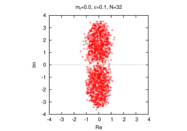
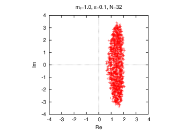
Figure 1: The scatter plot for the eigenvalues of the Dirac operator obtained during the complex Langevin simulation of the undeformed model (10) for $\varepsilon=0.1$ with $N=32$ (Left) and that of the deformed model defined by (13) and (14) for $\varepsilon=0.1$ with $m_{{\rm f}}=1.0$ and $N=32$ (Right).

In order to avoid this problem, we add a fermion bilinear term which deforms the Dirac operator (3), so that the partition function of the deformed model is defined as

$$\tilde{Z}=\int dX\,\tilde{w}(X)\ ,\quad\quad\tilde{w}(X)=\left(\det\tilde{D}\right)^{N_{{\rm f}}}e^{-(S_{{\rm b}}+\Delta S_{{\rm b}})}\ ,$$

$$\tilde{D}_{i\alpha,j\beta}=\sum_{\mu=1}^{4}(\Gamma_{\mu})_{\alpha\beta}\Big{(}(X_{\mu})_{ij}+M_{\mu}\delta_{ij}\Big{)}\ .$$ (13)

Note that the deformation explicitly breaks the SO(4) symmetry of the original model (1). Here we choose the parameters $M_{\mu}$ in such a way that the SO(4) symmetry is broken minimally. Taking account of the ordering (7), we can preserve an SO(3) symmetry at $\varepsilon=0$ by choosing

$$M_{\mu}=\left(0,0,0,m_{{\rm f}}\right)\ .$$ (14)

We can then ask whether the SO(3) symmetry of this deformed model is spontaneously broken in the large-$N$ limit.

In Fig. 1 (Right), we plot the eigenvalue distribution of the Dirac operator (13) obtained during the complex Langevin simulation of the deformed model for $\varepsilon=0.1$ with $m_{{\rm f}}=1.0$ and $N=32$. We find that the distribution is shifted in the real direction, which is understandable since, at large $m_{{\rm f}}$, the eigenvalue distribution of the Dirac operator would be distributed around $m_{{\rm f}}$. As a result, the distribution avoids the singularity even for $\varepsilon=0.1$ in contrast to the undeformed ($m_{{\rm f}}=0$) case. Therefore, we can extrapolate $\varepsilon$ to zero using data obtained with smaller $\varepsilon$ for finite $m_{{\rm f}}$. Eventually, we extrapolate the deformation parameter $m_{{\rm f}}$ to zero, and compare the results with the prediction (8) obtained by the GEM for the original model.

4 Results of our analysis

Let us recall that we have introduced an O($\varepsilon$) mass term (4) for the bosonic matrices, which breaks the SO(4) symmetry explicitly. In order to probe the SSB, we need to take the large-$N$ limit with fixed $\varepsilon$, and then make an extrapolation to $\varepsilon=0$ afterwards. In what follows, we present our results after taking the large-$N$ limit.

When we extrapolate $\varepsilon$ to zero, it is convenient to consider the ratio

$$\rho_{\mu}(\varepsilon,m_{{\rm f}})=\frac{\langle\lambda_{\mu}\rangle_{\varepsilon,m_{{\rm f}}}}{\sum_{\nu=1}^{4}\langle\lambda_{\nu}\rangle_{\varepsilon,m_{{\rm f}}}}\ .$$ (15)

This is motivated from the fact that the mass term (4) tends to make all the expectation values $\langle\lambda_{\mu}\rangle_{\varepsilon,m_{{\rm f}}}$ smaller than the value to be obtained in the $\varepsilon\rightarrow 0$ limit. By taking the ratio (15), the finite $\varepsilon$ effects are canceled by the denominator, and the extrapolation to $\varepsilon=0$ becomes easier.

In Fig. 2 (Left), we plot the ratio (15) against $\varepsilon$ for $m_{{\rm f}}=1.0$. Using the criterion proposed in ref. [6], we can decide which data points in the small $\epsilon$ region suffer from the singular drift problem and hence should be excluded from the extrapolation to $\epsilon=0$. We find that the fitting curves for $\rho_{1}(\varepsilon,m_{{\rm f}})$ and $\rho_{2}(\varepsilon,m_{{\rm f}})$ approach the same value at $\epsilon=0$, while the others approach smaller values. This implies that the SSB from SO(3) to SO(2) occurs in the deformed model.

Figure 2: (Left) The ratios $\rho_{\mu}(\varepsilon,m_{{\rm f}})$ obtained after taking the large-$N$ limit for the deformed model defined by (13) and (14) are plotted against $\varepsilon$ for $m_{{\rm f}}=1.0$. The lines represent fits to the quadratic form $a+b\varepsilon+c\varepsilon^{2}$. (Right) The extrapolated values $\lim_{\varepsilon\rightarrow 0}\rho_{\mu}(\varepsilon,m_{{\rm f}})$ for the deformed model defined by (13) and (14) are plotted against $m_{{\rm f}}^{2}$. The lines represent fits to the quadratic form $a+bx+cx^{2}$ with $x=m_{{\rm f}}^{2}$ using the data within the region $0.4\leq m_{{\rm f}}\leq 1.0$.

In Fig. 2 (Right), we plot the extrapolated values $\lim_{\varepsilon\rightarrow 0}\rho_{\mu}(\varepsilon,m_{{\rm f}})$ thus obtained against $m_{{\rm f}}^{2}$. We find that our results within $0.4\leq m_{{\rm f}}\leq 1.0$ can be nicely fitted to the quadratic behavior, which is motivated by a power series expansion of the expectation values $\langle\lambda_{\mu}\rangle_{\varepsilon,m_{{\rm f}}}$ with respect to $m_{{\rm f}}$. Extrapolating $m_{{\rm f}}$ to zero, we obtain $\lim_{m_{{\rm f}}\rightarrow 0}\lim_{\varepsilon\rightarrow 0}\rho_{\mu}(\varepsilon,m_{{\rm f}})=0.328(4),$ 0.326(2), 0.208(2), 0.133(2) for $\mu=1,2,3,4$, which shows that the SO(4) symmetry of the undeformed model ($m_{{\rm f}}=0$) is spontaneously broken down to SO(2). Moreover, using an exact result $\sum_{\mu=1}^{4}\langle\lambda_{\mu}\rangle=4+2r=6$ [8] for the present $r=1$ case, we obtain

$$\left\langle\lambda_{1}\right\rangle=1.97(2)\ ,\quad\left\langle\lambda_{2}\right\rangle=1.96(1)\ ,\quad\left\langle\lambda_{3}\right\rangle=1.25(1)\ ,\quad\left\langle\lambda_{4}\right\rangle=0.80(1)\ ,$$ (16)

which agree well with the results (8) obtained by the GEM. Here we emphasize that in the GEM, the true vacuum was determined by comparing the free energy obtained for the SO($2$) vacuum and the SO($3$) vacuum. In contrast, the CLM enables us to determine the true vacuum directly without having to compare the free energy for different vacua.

5 Summary and discussion

We have shown that the CLM can be successfully applied to a matrix model, in which the SSB of SO(4) is expected to occur due to the phase of the complex fermion determinant. For this success, it was crucial to overcome the singular-drift problem associated with the appearance of nearly zero eigenvalues of the Dirac operator. Our strategy was to deform the Dirac operator in such a way that the singular-drift problem is avoided while maintaining the qualitative feature of the vacuum as much as possible. Extrapolating the deformation parameter, we were able to obtain the order parameters, which turned out to be consistent with the prediction by the GEM.

The CLM with the proposed strategy can be directly applied to the type IIB matrix model, which is conjectured to be a nonperturbative formulation of type IIB superstring theory in ten dimensions [7]. While the SO(10) symmetry of the model is expected to be spontaneously broken down to SO(4) for consistency with our 4d space-time, the GEM predicts that it is spontaneously broken down to SO(3) rather than SO(4). It would be interesting to investigate this issue using the CLM extending the present work.

We consider that the same strategy would enable the application of the CLM to finite density QCD at low temperature and high density, where various exotic condensates are speculated to form due to the complex fermion determinant. We can try to find some deformations which allow us to extrapolate the deformation parameter to zero within the region of validity. Here the new criterion [6] for justifying the CLM should be useful, as it is the case in the present work [10].

References

- [1] G. Parisi, On complex probabilities, Phys. Lett. B 131 (1983) 393.
- [2] J. R. Klauder, Coherent state Langevin equations for canonical quantum systems with applications to the quantized Hall effect, Phys. Rev. A 29 (1984) 2036.
- [3] A. Mollgaard and K. Splittorff, Complex Langevin dynamics for chiral Random Matrix Theory, Phys. Rev. D 88 (2013) no.11, 116007 [arXiv:1309.4335 [hep-lat]].
- [4] J. Nishimura and S. Shimasaki, New insights into the problem with a singular drift term in the complex Langevin method, Phys. Rev. D 92 (2015) no.1, 011501 [arXiv:1504.08359 [hep-lat]].
- [5] G. Aarts, F. A. James, E. Seiler and I. O. Stamatescu, Complex Langevin: etiology and diagnostics of its main problem, Eur. Phys. J. C 71 (2011) 1756 [arXiv:1101.3270 [hep-lat]].
- [6] K. Nagata, J. Nishimura and S. Shimasaki, The argument for justification of the complex Langevin method and the condition for correct convergence, arXiv:1606.07627 [hep-lat].
- [7] N. Ishibashi, H. Kawai, Y. Kitazawa and A. Tsuchiya, A large N reduced model as superstring, Nucl. Phys. B 498 (1997) 467 [hep-th/9612115].
- [8] J. Nishimura, Exactly solvable matrix models for the dynamical generation of space-time in superstring theory, Phys. Rev. D 65 (2002) 105012 [hep-th/0108070].
- [9] J. Nishimura, T. Okubo and F. Sugino, Gaussian expansion analysis of a matrix model with the spontaneous breakdown of rotational symmetry, Prog. Theor. Phys. 114 (2005) 487 [hep-th/0412194].
- [10] Y. Ito and J. Nishimura, The complex Langevin analysis of spontaneous symmetry breaking induced by complex fermion determinant, arXiv:1609.04501 [hep-lat].
- [11] K. N. Anagnostopoulos, T. Azuma and J. Nishimura, A practical solution to the sign problem in a matrix model for dynamical compactification, JHEP 1110 (2011) 126. [arXiv:1108.1534 [hep-lat]].
- [12] E. Seiler, D. Sexty and I. O. Stamatescu, Gauge cooling in complex Langevin for QCD with heavy quarks, Phys. Lett. B 723 (2013) 213 [arXiv:1211.3709 [hep-lat]].