Equilibrium and dynamic pleating of a crystalline bonded network

Abstract

We describe a phase transition that gives rise to structurally non-trivial states in a two-dimensional ordered network of particles connected by harmonic bonds. Monte Carlo simulations reveal that the network supports, apart from the homogeneous phase, a number of heterogeneous “pleated” phases, which can be stabilised by an external field. This field is conjugate to a global collective variable quantifying “non-affineness”, i.e. the deviation of local particle displacements from local affine deformation. In the pleated phase, stress is localised in ordered rows of pleats and eliminated from the rest of the lattice. The kinetics of the phase transition is unobservably slow in molecular dynamics simulation near coexistence, due to very large free energy barriers. When the external field is increased further to lower these barriers, the network exhibits rich dynamic behaviour: it transforms into a metastable phase with the stress now localised in a disordered arrangement of pleats. The pattern of pleats shows ageing dynamics and slow relaxation to equilibrium. Our predictions may be checked by experiments on tethered colloidal solids in dynamic laser traps.

I Introduction

Fabricating complex shapes by folding or pleating a two-dimensional elastic manifold has recently emerged as a viable technological paradigm, applicable over a large range of length scales, from microns to nanometers origami1 ; origami2 ; origami3 ; irvine . A number of these innovative ideas are equally applicable for atomic crystals or for larger assemblies involving functionalized colloidal particles joined together using polymer tethers carpets or micron-sized lipid droplets bayley ; shape . To make such attempts feasible, one needs efficient ways to control local structural properties, preferably in a reversible way. Thus, microscopic understanding of the underlying thermodynamics and kinetics of these or similar local shape changes would be valuable.

In this paper, we study in detail equilibrium and dynamic aspects of a transition in a tethered network of colloidal particles – from a homogeneous to a heterogeneous phase containing an ordered arrangement of pleats. Within these pleats, the network penetrates itself, with parallel rows of vertices folding back to completely or nearly overlapping adjacent rows. These complex structures arise here spontaneously as a result of an underlying, equilibrium “first-order” phase transformation CL .

We show that pleating excitations are induced and controlled by a novel external field conjugate to a collective variable falk defined as follows. In earlier work, it was demonstrated that local displacements of particles in a crystal away from their ideal positions may be decomposed into affine and non-affine components sas1 ; sas2 ; sas3 . External stress couples to the affine part of the displacements. In analogy, one imagines an external field, which is conjugate to a global collective coordinate $X$, measuring non-affineness, to be defined explicitly later. This “non-affine” field, $h_{X}$, is realisable experimentally for colloidal solids using dynamic laser traps sas2 ; HOT . For small $h_{X}>0$, non-affine displacements, and consequently $X$, are enhanced in a controlled manner computable within a linear response framework. In a non-bonded conventional crystal, this leads to the creation of defects sas2 . The present paper is devoted to an analysis of the consequences of large positive $h_{X}$ in a connected network much beyond the linear response regime.

We consider a periodic lattice of point vertices in two dimensions (2d) that are connected to their nearest neighbours by harmonic springs. Crystalline 2d networks have been studied extensively in the past network ; pleats1 ; pleats2 , partly because of their biological significance (e.g. as a simple model for the spectrin network in red blood corpuscles) spectrin ; spectrin1 . Note that such a network has non-trivial properties, such as the presence of pleats, only when the bond length is random or exceeds the nearest neighbour distance set by the density pleats2 by a critical amount. In this case the network suffers an instability and catastrophic collapse. This is in stark contrast to the equilibrium first order transition CL in the presence of $h_{X}$ (and zero external stress) to an ordered pleated state that we describe, we believe for the first time, in the present work. For this transition, we obtain the relative free energies of the pleated phases as well as individual free energy barriers in quantitative detail – a first but essential step towards efficient control over their formation.

We use two distinct particle-based simulation techniques for this study. Monte Carlo (MC) simulations binder in combination with sequential umbrella sampling (SUS) SUS are used to compute the free energy landscape as a function of $X$ at various values of $h_{X}$. We show that SUS-MC simulations are able to detect metastable phases which are inaccessible by conventional MC. Free energies of interfacial structures between pleated and un-pleated regions of the lattice can also be investigated and energy barriers for the formation of the product phase determined. This advanced sampling method (SUS-MC) allows us to not only identify this as a first order phase transition but also to characterise the properties of the coexisting states separated by interfaces. This latter point is remarkable because we obtain explicitly an interface between an inhomogeneous state (i.e. the pleated state) and the normal crystal. Locating this interface is nontrivial and requires the computation of local stresses.

We use molecular dynamics (MD) simulations allen ; frenkel at constant particle number, total area and temperature (NAT) to reveal the kinetic aspects of this transition. In the MD simulation, the transformation shows features that are different from the thermodynamic first-order transition, as seen in SUS-MC. The transformation occurs at a larger value of $h_{X}$ and leads to a metastable phase. We show, in this work, the strong interplay between kinetics and thermodynamic phase behaviour. The equilibrium pleated states are heterogeneous phases which are quite difficult to realise via a kinetic pathway. Conversely, the nature of the metastable states obtained in the kinetic transition can only be understood if one is able to identify the underlying phase transition through SUS-MC.

We have carried out the simulations for both the pure, non-self avoiding network as well as a model where the vertices of the network are decorated with finite-sized colloidal particles. On a qualitative level, the findings for both models are similar.

The rest of the paper is organised as follows. Section II introduces the local and global non-affine parameters, $\chi({\bf R})$ and $X$, as well as the field $h_{X}$ conjugate to the latter. Moreover, the details of the model solids and simulation methodology are presented here. Then, in Sec. III, a comprehensive exposition of our results for the network solid is given. We report results for analytic calculations for small $h_{X}$, ground states and finite temperature phases and the dynamical transition in this model. We end the paper with a summary and conclusions as well as an outlook for future work.

II Models, Formalism and Simulation Details

In this section, we commence our discussion by first introducing the non-affine field $h_{X}$ and the model Hamiltonians followed by a description of the simulation methodologies used.

II.1 The model Hamiltonian with the non-affine field

Consider a reference configuration of $N$ particles where the particle with index $i$ ($i=1,...,N$) is located at position ${\bf R}_{i}$. A displacement of particle $i$ from its position on the reference lattice is given by ${\bf u}_{i}={\bf r}_{i}-{\bf R}_{i}$, with ${\bf r}_{i}$ the instantaneous position of the particle. Now within a neighborhood $\Omega$ around particle $i$, we define relative atomic displacements ${\bf\Delta}_{j}={\bf u}_{j}-{\bf u}_{i}$ with particle $j\neq i\in\Omega$. The “best fit” falk local affine deformation ${\mathsf{D}}$ is the one that minimizes $\sum_{j}[{\bf\Delta}_{j}-{\mathsf{D}}({\bf R}_{j}-{\bf R}_{i})]^{2}$ with the non-affinity parameter $\chi({\bf R}_{i})>0$ being the minimum value of this quantity. The minimisation procedure amounts to projecting sas1 ${\bf\Delta}_{i}$ onto a non-affine subspace defined by a projection operator ${\mathsf{P}}$ such that $\chi({\bf R}_{i})={\bf\Delta}^{\rm T}{\mathsf{P}}{\bf\Delta}$ where $\Delta$ is the column vector constructed out of the ${\bf\Delta}_{i}$. In the projector ${\mathsf{P}}={\mathsf{I}}-{\mathsf{R}}({\mathsf{R}}^{\rm T}{\mathsf{R}})^{-1}{\mathsf{R}}^{\rm T}$, the $Nd\times d^{2}$ elements of ${\mathsf{R}}$ are given by ${\mathsf{R}}_{j\alpha,\gamma\gamma^{\prime}}=\delta_{\alpha\gamma}R_{j\gamma^{\prime}}$ (here, the central particle $i$ is taken to be at the origin). This projection formalism is perfectly general and can be carried through for any lattice in any dimension.

Once the dynamical matrix ${\mathcal{D}}({\bf q})=v_{BZ}^{-1}\langle{\bf u}_{\bf q}{\bf u}_{\bf-q}\rangle$ is obtained ($v_{BZ}$ is the volume of the Brillouin zone), we can calculate the ensemble average of the non-affine parameter $\langle\chi\rangle$ using a coarse graining procedure outlined in sas1 ; sas2 . We include this in brief here for completeness.

We define the coarse grained correlations, $C_{i\alpha,j\beta}=\langle\Delta_{i\alpha}\Delta_{j\beta}\rangle$ where as before the Roman indices denote particles and the Greek ones denote coordinates. The particles $i,j$ both belong inside the neighborhood $\Omega$ of particle $0$. Substituting the definition of the displacement differences $\Delta_{i\alpha}=u_{i}^{\alpha}-u_{0}^{\alpha}$ we obtain sas1 ,

$$C_{i\alpha,j\gamma}=\int\frac{d{\bf q}}{v_{BZ}}\,{\mathcal{D}}^{-1}_{\alpha\gamma}({\bf q})(e^{i{\bf q}\cdot{\bf R}_{j}}-e^{i{\bf q}\cdot{\bf R}_{0}})(e^{-i{\bf q}\cdot{\bf R}_{i}}-e^{-i{\bf q}\cdot{\bf R}_{0}})$$

The ensemble average of $\langle\chi\rangle$ is then given by ${\rm Tr}~{}{\mathsf{P}}{\mathsf{C}}{\mathsf{P}}$, where ${\mathsf{P}}$ is the projection operator. The non-trivial eigenvalues $\sigma_{\mu}$ of ${\mathsf{P}}{\mathsf{C}}{\mathsf{P}}$ and their corresponding eigenvectors are the non-affine modes of the lattice. For example, in the triangular lattice there are $8$ such modes when $\Omega$ corresponds to the nearest neighbour shell. The orthogonal subspace, i.e. the affine displacements, are spanned by the non-trivial eigenvectors of $(1-{\mathsf{P}}){\mathsf{C}}(1-{\mathsf{P}})$ and correspond to the usual volumetric, uniaxial and shear strains together with local rotations. The non-affine field does not affect the statistics of the affine part of the displacements to linear order in $h_{X}$. Space-time correlation functions of both affine and non-affine variables can also be obtained using a similar procedure sas1 ; sas2 .

In order to selectively excite lattice distortions that enhance non-affine displacements, we introduce an extended microscopic Hamiltonian sas2 involving the thermodynamic conjugate variables $h_{X}$ and $X$, with $X=N^{-1}\sum^{N}_{i}\chi({\bf R}_{i})$. In analogy to conjugate variables like stress-strain or pressure-volume, we add the product of $h_{X}$ and $X$ to the Hamiltonian:

$${\cal H} = {\cal H}_{0}-Nh_{X}X$$

$$= {\cal H}_{0}-h_{X}\sum_{i}^{N}\sum_{jk\in\Omega}({\bf u}_{j}-{\bf u}_{i})^{\rm T}{\bf P}_{j-i,k-i}({\bf u}_{k}-{\bf u}_{i}).$$

Here, ${\cal H}_{0}$ represents the Hamiltonian of any standard solid.

The second term in Eq. (LABEL:hamil_gen), $-Nh_{X}X$, involves appropriate Cartesian components ${\bf P}_{ij}$ of the projection operator ${\mathsf{P}}$ that couple to the relevant displacement differences. Note that the ${\bf P}_{ij}$ are constant parameters that only depend on the position vectors of the reference configuration, ${\bf R}_{i}$. The size of the coarse-graining volume $\Omega$ surrounding particle $i$ is set by the range of the interaction. In the rest of this paper, we take $\Omega$ as the nearest neighbour shell. A positive value of the non-affine field $h_{X}$ enhances non-affine distortions of the lattice sas1 ; sas2 , namely, fluctuations in particle positions projected onto a subspace spanned by those eigen-distortions of $\Omega$ that cannot be represented as combination of affine deformations.

We describe below our network model. The reference lattice structure $\{{\bf R}_{i}\}_{i=1,...,N}$ is an ideal triangular lattice. The Hamiltonian of this model is that of a standard network of point non self-avoiding vertices connected by harmonic bonds network ,

$${\cal H}_{0} = \sum^{N}_{i=1}\frac{{\bf p}_{i}^{2}}{2m}+\frac{K}{2}\sum_{i=1}^{N}\sum_{j\in\Omega,i<j}(|{\bf r}_{j}-{\bf r}_{i}|-|{\bf R}_{j}-{\bf R}_{i}|)^{2}$$

with ${\bf p}_{i}$ the momentum, $m$ the mass, ${\bf r}_{i}$ the instantaneous position, and ${\bf R}_{i}$ the reference position of vertex $i$ as before. The length scale is set by the lattice parameter $l$, the energy scale by $Kl^{2}$, and the time scale by $\sqrt{m/K}$. We use those as our units in the following, effectively setting $l=m=K=1$. A dimensionless inverse temperature is given by $\beta=Kl^{2}/k_{B}T$, with $k_{B}$ the Boltzmann constant.

For some of the calculations reported here, we attach finite sized repulsive particles with every vertex. The Hamiltonian is therefore augmented to ${\cal H}_{0}^{\prime}={\cal H}_{0}+{\cal H}_{WCA}$ with

$${\cal H}_{WCA} = \sum_{i=1}^{N-1}\sum_{j>i}v_{\rm WCA}(r_{ij})$$ (2)

The interaction potential for a pair of particles, separated by a distance $r$, is

$$v_{\rm WCA}=4\phi\left[\left(\frac{r_{0}}{r}\right)^{12}-\left(\frac{r_{0}}{r_{c}}\right)^{12}-\left(\frac{r_{0}}{r}\right)^{6}+\left(\frac{r_{0}}{r_{c}}\right)^{6}\right]$$ (3)

for $r\leqslant r_{c}=2^{\frac{1}{6}}r_{0}$ and $v_{\rm WCA}=0$ for $r>r_{c}$. We use $\phi=1$ and $r_{0}=0.6l$, respectively.

II.2 Simulation Details

We perform molecular dynamics simulations as well as Monte Carlo in combination with sequential umbrella sampling of the regions of configuration space that are otherwise inaccessible using simple MC or MD simulation techniques.

Molecular Dynamics.

MD simulations in the canonical ensemble, i.e. at constant number $N$ of vertices, area $A$ and temperature $T$, were done using a leapfrog algorithm, coupling the system to a Brown and Clarke thermostat allen ; frenkel . The size of the systems ranges from $N=100$ to $N=40000$ vertices. Typically, unless otherwise stated, we used an MD time step of $\delta t=0.002$ and inverse temperature $\beta=200$. These parameters are the same even when repulsive, WCA particles are attached to the vertices. Typically, the solid was held for $5\times 10^{5}$ MD steps followed by the collection of data for further $5\times 10^{5}$ MD steps at an interval of $1000$ steps.

Sequential Umbrella Sampling.

Standard Metropolis Monte Carlo frenkel ; binder is inefficient in sampling systems with free energy barriers separating different regions in configuration space. SUS is an advanced sampling technique SUS ; frenkel ; binder that ensures good sampling of the entire range of pertinent states. Our implementation of SUS-MC in the $NAT$ ensemble involves dividing the range of the relevant order parameter, $X$, into small windows to be sampled successively starting at $X=0$. Histograms denoted by $H(n)$ keep track of how often each value of $X$ within the $n$th window is realized, with $H(n)_{L}$ and $H(n)_{R}$ representing the left and right boundaries of the $n$th histogram. Now, a predetermined number of MC moves are attempted per window. MC moves resulting in $X$ within the chosen window are accepted or rejected using the conventional Metropolis criterion and the relevant histograms are modified accordingly. Any moves leading to values of $X$ outside the chosen window are rejected with appropriate modification of the histograms at the boundaries to ensure detailed balance SUS . Finally, the un-normalized relative probability distribution of $X$ can be computed using,

$$\frac{P(X_{n})}{P(X_{0})}=\frac{H(0)_{R}}{H(0)_{L}}\cdot\frac{H(1)_{R}}{H(1)_{L}}\cdots\frac{H(n)_{R}}{H(n)_{L}}.$$

The SUS-MC runs, for the network model, were done for systems with $N=900$ at $\beta=200$ and density $\rho=1.1547$ (which corresponds to our choice $l=1$ for the lattice parameter). For systems with $N=900$, we considered the range between $X=0.0$ and $X=1.0$ and divided this into $500$ sampling windows with $8\times 10^{7}$ MC moves attempted in each window. In each MC move, maximal particle displacements of $0.2\,l$ along the $x$ and $y$ directions are allowed. Apart from simulations with $N=900$ vertices, systems with $N=100$ and $N=400$ were studied using SUS-MC. As the variance of the parameter $X$ is proportional to inverse of the system size sas2 , the range of $X$ for sampling was chosen accordingly, viz. $0.0\leq X\leq 3.0$ for $N=100$, $0.0\leq X\leq 1.5$ for $N=400$, and $0.0\leq X\leq 1.0$ for $N=900$. Also for $N=100$ and $N=400$, the range of $X$ was divided into 500 sampling windows with $8\times 10^{7}$ MC trial moves in each window.

III Results

III.1 Crystal properties in the presence of small $h_{X}$

We first study the properties of our model solid in the low temperature limit, where a harmonic approximation becomes exact even in the presence of the non-affine field $h_{X}$. Indeed, the complete low-$T$ statistical mechanics of the system can be obtained as long as the periodic crystalline phase is stable. Therefore we begin by first presenting analytic results for finite values of $h_{X}$ sas1 ; sas2 ; sas3 in the ideal crystal. These calculations provide an estimate of the critical value, $h_{X}^{0}$, at which the crystal becomes unstable under the application of the non-affine field.

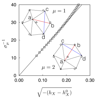
Figure 1: Plots of inverse eigenvalues $\sigma_{1}^{-1}$ and $\sigma_{2}^{-1}$ as a function of $h_{X}$, corresponding to the two degenerate non-affine modes at the lowest energy (filled squares). The solid curve is a linear fit through the last three data points. The lattice distortions corresponding to these modes are illustrated in the inserted sketches. Note that in each case nearest neighbours $a,b$ (red lines) move apart while next nearest neighbours, $c,d$ (blue lines) come closer (see text).

In order to understand how crystal properties are affected by the non-affine field, $h_{X}$, we calculate the eigenvalues of the dynamical matrix born ; harmdyn and the corresponding eigenvectors. The dynamical matrix is obtained from the Fourier transform of the Hessian ${\cal D}({\bf R},{\bf R}^{\prime})=\partial^{2}{\cal H}/\partial{\bf u}({\bf R})\partial{\bf u}({\bf R}^{\prime})$. The full expression for ${\cal D}$ in the presence of a non-affine field $h_{X}$ can be worked out in a straightforward manner and one obtains,

$$\mathcal{D}=K\left(\begin{array}[]{cc}3-2\mathcal{A}_{1}-\mathcal{A}_{2}-\frac{2h_{X}}{K}\mathcal{A}_{X}&\sqrt{3}\mathcal{A}_{3}\\ \sqrt{3}\mathcal{A}_{3}&3-3\mathcal{A}_{2}-\frac{2h_{X}}{K}\mathcal{A}_{X}\end{array}\right),$$

with

$$\mathcal{A}_{1} = \cos(q_{x}),$$

$$\mathcal{A}_{2} = \cos(\frac{1}{2}q_{x})\cos(\frac{\surd 3}{2}q_{y}),$$

$$\mathcal{A}_{3} = \sqrt{3}\sin(\frac{1}{2}q_{x})\sin(\frac{\surd 3}{2}q_{y}),$$

$$\mathcal{A}_{X} = \frac{1}{6}\Bigg{\{}\left[60-28\cos(q_{x}l)-56\cos\Big{(}\frac{q_{x}l}{2}\Big{)}\cos\Big{(}\frac{q_{y}\sqrt{3}l}{2}\Big{)}\right]$$

$$+\left[4\cos(2q_{x}l)+8\cos(q_{x}l)\cos(q_{y}\sqrt{3}l)\right]$$

$$+\left[8\cos\Big{(}\frac{q_{x}3l}{2}\Big{)}\cos\Big{(}\frac{q_{y}\sqrt{3}l}{2}\Big{)}+4\cos(q_{y}\sqrt{3}l)\right]\Bigg{\}}.$$

Note that the leading order term in $\mathcal{A}_{X}(q)$ is of order ${\mathcal{O}}(q^{4})$, so that $h_{X}$ does not contribute to the speed of sound or to elastic constants.

Increasing $h_{X}$ enhances $\langle\chi\rangle$ locally, which is associated with a softening of certain phonon modes. At small ${\bf q}$, the transverse phonon modes are softened showing that the solid becomes nearly unstable to large wavelength shear modes. We find that most of this contribution comes from the two softest non-affine modes, i.e. the eigenvectors of ${\mathsf{P}}{\mathsf{C}}{\mathsf{P}}$ with the smallest eigenvalues $\sigma_{\mu}$ ($\mu=1,2$). These two eigenvalues are identical and the corresponding modes are illustrated in the sketches of Fig. 1: distortions with respect to the reference configuration (open circles) are generated where nearest neighbours $a,b$ move away from each other while next-nearest neighbours $c,d$ come closer tending to nucleate a dislocation dipole sas2 . Note that any linear combinations of these modes are also degenerate and so the direction of the modulation wavenumber, with magnitude $\chi^{-1/2}$, varies in space pointing randomly in all directions consistent with crystal symmetry.

In Fig. 1, we plot the reciprocal of the largest non-affine eigenvalue ($\sigma_{\mu}$ with $\mu=1,2$) as a function of $h_{X}$. As $h_{X}$ increases, this eigenvalue vanishes as $\sqrt{h_{X}-h_{X}^{0}}$ pointing to an underlying saddle-node bifurcation point beyond which a crystalline solid cannot exist sas1 . Similar behavior is shown by all the eigenvalues (not shown) corresponding to the non-affine modes sas2 . As we can estimate from the plot, the eigenvalues $\sigma_{\mu}$ with $\mu=1,2$ diverge around $h_{X}^{0}=0.072$ – the limit of stability of the crystal in a non-affine field.

III.2 Pleated configurations at $T=0$

Having considered the ideal crystalline ground state of the non-self-avoiding triangular network, we now ask whether additional low-energy configurations exist. Indeed, we show that configurations containing one or more pleats, as illustrated in Fig. 2, are also possible. Within a pleat, two rows of vertices overlap producing a band of twice the local stiffness. Note that the pleated configuration remains two-dimensional. While similar pleated structures have been reported network ; pleats1 ; pleats2 for such networks under compression or with disorder, to the best of our knowledge, the existence of these states for regular crystalline networks has never been commented upon before. As explained in Fig. 2a., in a pleated state no bond is stretched or compressed. A pleated row of vertices does not destroy local crystalline order and can be distinguished only by a high value of local $\chi$, pointing out that a finite non-affine displacement is necessary to produce a pleat. The displacement ${\bf u}$ however becomes a multi-valued function of the coordinates at the location of the pleats with each of the two values corresponding to the two distinct “leaves” of the pleat. Since the lattice is stiffer at the pleats these regions are also regions of enriched stress.

A positive $h_{X}$ encourages the formation of pleats. In a solid of size $L$, internal strains $\varepsilon_{int}\sim 1/L$, however, need to be introduced to fit the the pleated lattice back into the box, making configurations with a large number of pleats energetically unfavourable. Consider, for the moment, only pleats of full rows, all in the same direction, then having $p$ pleats requires a strain of $p/L$ elsewhere, hence elastic energy $\sim L^{2}(p/L)^{2}~{}\sim p^{2}$. However, we gain an energy $\sim h_{X}pL$ from the field term as $\chi$ is increased to ${\mathcal{O}}(1)$ in an area of order $pL$. Equating the two predicts $p\sim h_{X}L$ or $p/L\sim h_{X}$, i.e. a finite fraction of pleats that increases linearly with $h_{X}$. At $h_{X}=0$ one has competition between energy $\sim p^{2}$ and entropy $\sim p\ln L$ and thus expects $p\sim\ln L$, hence $p/L\to 0$ as $L\to\infty$.

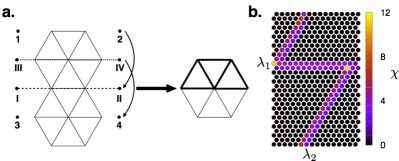
Figure 2: a. Schematic illustration of a pleat in the triangular lattice as an origami fold. A “valley” fold at $\mathsf{I}-\mathsf{II}$ and a “mountain” fold at $\mathsf{III}-\mathsf{IV}$ bring the vertices at $\mathsf{I},\mathsf{II}$ and $1,2$ as well as $\mathsf{III},\mathsf{IV}$ and $3,4$ together to obtain the final two-dimensional configuration shown on the right. Note that the pleated configuration has two layers less and $7$ overlapped bonds together with $5$ overlapped vertices. Such an operation can be continued along a crystalline row of vertices creating a complete pleat. Note further that none of the bonds in the pleat are either stretched or compressed. b. An originally $18\times 32$ lattice with one horizontal and one $60^{\circ}$ pleat of amplitudes $\lambda_{1}=\lambda_{2}=2$ lattice spacings. The vertices are shown as filled circles coloured according to the value of local $\chi$. The pleats do not destroy local crystalline order but have large local $\chi$ values (color bar).

In Fig. 2b, we illustrate this with two pleats, one horizontal and the other tilted at an angle of $60^{\circ}$. We create these configurations by shifting rows of vertices either downwards or to the left by amounts $\lambda_{1}$ and $\lambda_{2}$ respectively. Here $\lambda_{1}=\lambda_{2}=2$ lattice spacings. The local $\chi$ is a quadratic function of both $\lambda_{1}$ and $\lambda_{2}$. Note that internal strains and the term proportional to $h_{X}$ in ${\mathcal{H}}$ determine the relative stability of the pleated configurations. The network responds to $h_{X}$ by either increasing the density of the pleats or by introducing side branches at $60^{\circ}$ (or equivalently $120^{\circ}$) to the horizontal. Large $h_{X}$ favours a large number of pleats and in that regime several configurations may have the same average non-affineness $X$ and, at the same time, be degenerate in energy. In the next section we show that these pleated configurations of the crystalline network survive at non-zero temperatures and lead to interesting phase behaviour.

III.3 The phase transition at $T>0$

In this section we study in detail the phase transition from an un-pleated solid to one with pleats at finite temperatures. This transition can be located by SUS-MC which gives at a given value of $h_{X}$ the probability $P(X)$ to find the system in a state with a certain value of $X$. The logarithm of this probability is directly related to the corresponding free energy, $F(X)=-k_{B}T\ln P(X)+C$ (with $C$ a constant).

Figure 3a displays $-\ln P(X)$ for the system with $N=30\times 30$ lattice sites at different values of $h_{X}$. All the distributions exhibit a first minimum around $X=0.05$ consistent with our results for the ideal network in the harmonic approximation sas2 . A saddle point also appears at $X_{\rm saddle}\approx 0.1$ which is almost independent of $h_{X}$. For $X>X_{\rm saddle}$, the function $-\ln P(X)$ first decreases until a second minimum is reached. At higher values of $X$ more minima and shoulders can be discerned in the distributions; at high values of $h_{X}$ these lie below the first two minima and thus correspond to the stable states in this regime.

In Fig. 3b, $P(X)$ at $h_{X}=0.025$ for various system sizes $N$ is plotted. In a conventional first-order phase transition CL , $P(X)$ sharpens with increasing system size such that $-N^{-1}\ln(P(X,N))$ approaches its thermodynamic limit. In our system, while $P(X)$ does become narrower with increasing $N$, detailed features of $P(X)$ depend non-trivially on the system size. Indeed for larger system sizes, additional minima appear that correspond to domain configurations not possible for smaller sizes. One of the great advantages of the SUS-MC method is that configurations that contribute to $P(X)$ in each range are directly available.

Snapshots for different values of $X$ at $h_{X}=0.030$ (as marked in Fig. 3a by black dots) are displayed in Fig. 3c. Here each vertex is represented as a filled circle and coloured according to the local value of $\log_{10}\chi$. While the configuration corresponding to the first minimum in $-\ln(P(X))$ is a homogeneous crystal, the one corresponding to the second minimum is an inhomogeneous phase where a band of vertices with a high positive $\chi$ value percolates through the crystal. The latter band does not simply consist of two lattice rows, as the snapshot may suggest. While the two rows fit perfectly into the hexagonal structure, each of the two rows consist of a pair of overlapping rows, i.e. a pleat. At higher values of $X$, in addition to the horizontal pleat, side branches form at an angle of $60^{\circ}$ with a geometry similar to that used in the $T=0$ calculation. On further increasing $X$, the side branches cross the main band such that they also percolate through the system.

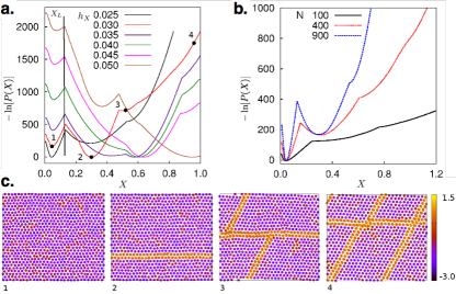
Figure 3: a. $-\ln(P(X))$ obtained from sequential umbrella sampling of a $30\times 30$ lattice at various values of $h_{X}$. The first minimum always corresponds to the ideal triangular lattice. As $h_{X}$ increases, the crystalline solid is destabilised with respect to other minima at larger $X$. The vertical black line marks the position of the first saddle point showing that it is approximately independent of $h_{X}$. b. $-\ln(P(X))$ obtained from sequential umbrella sampling of $10\times 10$, $20\times 20$, $30\times 30$ and $50\times 50$ lattices at $h_{X}=0.025$ showing that the $P(X)$ becomes sharper with increasing system size. c. Particle configurations at specific points of $-\ln(P(X))$ for the $30\times 30$ solid as indicated by dots in a. The colours represent the local values of $\log_{10}\chi$.

Is there a finite temperature phase transition from a homogeneous crystalline phase to an inhomogeneous phase with a pleat of “non-affine” vertices? At such a transition, the probability distribution $P(X)$ would exhibit two peaks with the area under both peaks being equal binder . As one can infer from Fig. 3a, this happens for a value of $h_{X}$ between 0.025 and 0.030. To obtain an estimate of the coexistence value for $h_{X}$, one can use histogram reweighting and deduce from a reference distribution at $h_{X}^{(1)}$, $P(X,h_{X}^{(1)})$, the distribution at $h_{X}^{(2)}$ via

$$-\ln P(X,h_{X}^{(2)})=-\ln P(X,h_{X}^{(1)})+\beta\left[h_{X}^{(2)}-h_{X}^{(1)}\right]NX\,.$$ (4)

Eq. (4) may now be used to determine the distribution $P(X,h_{X}^{\rm coex})$ for which the area under the peaks corresponding to the coexisting phases is equal. We accomplish this using an iterative procedure where successive refinements of $h_{X}^{\rm coex}$ are obtained from SUS-MC simulations at a previously estimated values of $h_{X}^{\rm coex}$. From this procedure we find $h_{X}^{\rm coex}=0.027$. We check that the final $P(X,h_{X}^{\rm coex})$ shows two peaks with equal area under them as required for co-existence (see Fig. 4a). States in the two-phase region (e.g. those points marked as C1, C2, and C3 in the figure) are also visible. Here, the two phases are at coexistence and separated from each other by an interfacial region. As the snapshots for the states C1, C2, and C3 show the pleat does not percolate through the system in the two-phase region and remains as a droplet terminated at two opposite vertices by the presence of the homogeneous crystal phase. Local $\chi$ is a convenient collective variable useful for characterising pleats. However, the thermodynamic variable which ought to show the interface between the homogeneous crystal and the inhomogeneous pleated phase is the space dependent, complex amplitude of the appropriate vertex density modulation. This is computationally difficult to obtain. Fortunately, as we show below, the local (uniaxial) stress distribution works just as well.

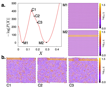
Figure 4: a. $-\ln P(X)$ is plotted as a function of $X$ at $h_{X}=0.027$, where the crystal and the inhomogeneous phase with a non-affine stripe of particles are at coexistence. b. Configuration snapshots with $\log_{10}\chi$ colormap corresponding to the states indicated in a. While the snapshots C1, C2, C3 represent instantaneous configurations, the snapshots M1 and M2 were obtained from a time average over $10^{4}$ subsequent configurations.

In Fig. 5 we demonstrate that the two phases at coexistence (Fig. 4) differ from each other with respect to the distribution of local stresses frenkel at coexistence, $P(\sigma)$, where $\sigma=\sigma_{xx}-\sigma_{yy}$, the deviatoric or uniaxial stress component. The distribution for the inhomogeneous phase (M2) has its maximum at the negative value $\sigma=-4\times 10^{-5}$ and is asymmetric, with a pronounced excess contribution at positive values of $\sigma$. The latter asymmetry reflects the localization of stresses in the pleat with a high value of $\log_{10}\chi$ (see snapshot corresponding to M2 in Fig. 4). In contrast, the distribution corresponding to M1 is symmetric and its maximum is at the positive value $\sigma=2\times 10^{-5}$. The corresponding snapshot indicates a homogeneous distribution of stresses. Thus, the two phases at M1 and M2 differ with respect to the average stress value and the localization of stress. In the M2 phase, the average stress value in the pleated region where the stress is localized is similar to that of the homogeneous M1 phase. All this is reflected in the snapshots corresponding to the two-phase region (C1, C2, and C3). Now the interfaces between the coexisting phases are clearly visible (dashed red lines in the plot of configuration C1, C2 and C3). While in the M1 phase stress is distributed throughout the crystal, in the M2 phase, it is eliminated from the un-pleated part and concentrated mostly at the pleat. There are two interfaces due to periodic boundary conditions and the amount of the two phases at a given state is controlled by the lever rule. Consequently, the free energy decreases linearly from state C1 to C3 (see Fig. 4), although the total area of the interfaces is constant for these three states. In the periodically repeated system, the M2 phase becomes a vertical stripe of undistorted network punctuated by a parallel array of horizontal pleats at regular intervals. Thermal undulations along the interfaces are also visible. In summary, Fig. 5 demonstrates that the order parameter of the transition from the homogeneous crystal to one with stress localisation within pleats can be connected to distribution of local stresses. We end this section with a comment on $P(\sigma)$ from our simulations. Fig.5 suggests that the $\sigma\to-\sigma$ symmetry is broken at $\varepsilon=0$. To obtain a complete description one would need to sample all degenerate, globally rotated copies of the crystal and also evaluate the full stress tensor $\sigma_{ij}$. This is however not necessary for our purpose here.

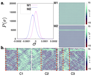
Figure 5: Distribution of local stresses $P(\sigma)$ corresponding to the minima M1 and M2, indicated in Fig. 4. The snapshots correspond to those in Fig. 4 but now the colormap represents the local stresses.

III.4 Dynamical transition and plastic deformation

In the last section we studied the properties of the pleated configurations showing that they form the stable equilibrium phase beyond a first order transition from an un-pleated to a pleated phase, which occurs in our network solid at $h_{X}=h_{X}^{\rm coex}\approx 0.027$ when $\beta=200$. How can such configurations form dynamically? We turn now to study this kinetic transition.

We have mentioned before that pleated configurations imply a multi-valued displacement field. Obviously, such a configuration cannot be represented as a linear combination of hydrodynamic phonon fluctuations of the network. Pleated configurations therefore need to form by the nucleation and growth of non-hydrodynamic, localized droplets. Incomplete pleated regions surrounded by a strained network have been observed and described in detail in the last subsection (see for example the C1 configuration in Fig. 4). For values of $h_{X}$ at which pleated states become globally stable, such droplet configurations, which lie in the saddle region in-between minima corresponding to un-pleated and pleated states cost extremely high free energy. Such high barriers prevent the equilibrium transition from occurring in MD simulations.

A dynamical transition at $T>0$ to a pleated configuration is possible only when $h_{X}$ becomes sufficiently large so that the lattice is close to being (but not quite!) locally unstable and the free energy barrier is substantially reduced. In Fig. 6b, we have plotted $h_{X}$ against $\langle X\rangle$ obtained from SUS-MC. The $\langle X\rangle$ values were obtained by a histogram reweighting method. Together with these results, we have also plotted results from MD simulations of the same network where $\langle X\rangle$ now represents an average over the MD simulation time. The MD and the SUS-MC results both show a jump in $\langle X\rangle$ at the pleating transition. However, the transition in MD occurs at a much larger value of $h_{X}$ showing that for a large range of $h_{X}$, the un-pleated state remains metastable. Note also that the value of $\langle X\rangle$ in the un-pleated state just before the dynamical transition is roughly equal to the value at the saddle point as shown in Fig. 3. A Lindemann like criterion linde ; CL viz. $X=X_{L}=X_{\rm saddle}$ just below the transition in the crystal phase is thus operative at this kinetic transition. Finite size effects in the MD simulations roughly follow those in the MC consistent with the shift of the position of the saddle point to smaller $X$ values (see Fig. 3b) with increasing $N$.

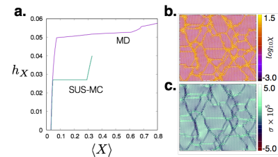
Figure 6: a. $h_{X}$ as function of $\langle X\rangle$ for both SUS-MC and MD simulations. b. and c. Configurations with vertices coloured according to $\log_{10}\chi$ and $\sigma\times 10^{5}$ obtained after the dynamical transition at $h_{X}=0.06$.

Configurations obtained just after the transition, at $h_{X}=0.06$, are plotted in Fig. 6b as both local $\chi$ and $\sigma$ maps. While pleated regions of higher local stress similar to the SUS-MC results are also seen here, the arrangement of the pleats is disordered. Close examination of the configurations also suggests that some of the pleated regions are amorphous. This may be understood as follows. As soon as the thermal energy required to cross the free energy barrier is available, the solid begins to form local pleats. Since many equivalent pleated states are equally stable at these high values of $h_{X}$ deep within the equilibrium phase boundary, the solid locally chooses between the several degenerate pleated states and relaxes, typically, to the nearest metastable free energy minimum. Further relaxation to the true equilibrium ground state, however, now needs large scale rearrangements of the network. As a consequence, the pleated solid shows ageing dynamics.

To show this, we compute the overlap function $Q(t)=N^{-1}\sum_{i}^{N}w(|{\bf r}_{i}(t)-{\bf r}_{i}(t_{w})|)$ for all vertices with local $\chi\geq\chi_{cut}=1$. The weight function $w(x)$ is zero or $1$ depending on whether $x>a$ or $x\leq a$, with $a$ being some predetermined length, smaller than the lattice spacing $l$; we choose $a=0.1l$. For a fixed value of $h_{X}=0.06$, starting from an initial crystalline structure, the system is allowed to relax for a “waiting” time $t_{w}$, before $Q(t)$ is computed. To obtain good statistics, $Q(t)$ is averaged over many independent runs.

In Fig. 7a, we plot $Q(t)$ for five values of $t_{w}$ spanning three orders of magnitude. In each case $Q(t)$ shows an initial rapid decrease to a plateau value, then slow relaxation in the plateau followed by an eventual escape away from the plateau at large times. $Q(t)$ depends on both $t$ and the waiting time $t_{w}$ implying that the system shows ageing behaviour. For a process where the system relaxes quickly to a steady state configuration, $Q(t)$ at long times always has a non-zero limiting value. To illustrate this, we plot in Fig. 7a $Q(t)$ for all the vertices in the crystalline network at a lower $h_{X}=0.02$. The long time behaviour of $Q(t)$ in this case is very different, saturating to a constant value. On the other hand, for a system showing complex dynamics requiring long range (and time consuming) particle rearrangements $Q(t)$ relaxes to a plateau first but then eventually decays to zero, on a timescale that grows with $t_{w}$. To distinguish between these behaviours, we plot $Q(t)$ against the scaled time $t^{*}=(t-t_{w})/t_{w}$ in Fig. 7b. The data collected over all three decades of $t_{w}$ collapse on a single curve which decays to zero at large values of $t^{*}$ showing that the phase transition kinetics bears strong resemblance to relaxation in a complex landscape.

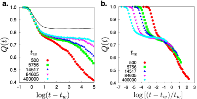
Figure 7: a. Ageing plot for the overlap function, $Q(t)$ as a function of $\ln t$ for several waiting times $t_{w}$ (see text). The black curve shows $Q(t)$ for a crystalline lattice i.e. at a lower value of $h_{X}=0.02$ b. Scaling collapse of the overlap function. The data is from MD simulations of a $20\times 20$ lattice at $h_{X}=0.06$, averaged over $60$ independent realizations.

All the results described so far correspond to the pleating transition in a non-self avoiding, 2d triangular crystalline network. If one thinks of the vertices as colloidal particles, then one might construct such a system experimentally and apply the non-affine field $h_{X}$ using dynamic laser traps in the fashion described in detail in Ref. sas2 Of course, colloidal particles are self-avoiding and will have an excluded volume. This should alter the properties of the pleats. Does it also suppress the pleating transition completely? We now show that while the detailed configuration of the pleats are affected because particles cannot overlap, this does not change any of the equilibrium or dynamic results substantially. While a complete overlap is impossible, particles occupy positions determined by a compromise between the bonding and the non-bonding, hard-core repulsion.

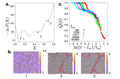
Figure 8: a. $-\log P(X)$ at $h_{X}=0.054$, obtained using SUS-MC simulations of a $30\times 30$ lattice with vertices occupied by particles interacting via an additional hard core WCA repulsion. b. Configurations from the SUS-MC simulations at three different values of $X$ shown in a. by black dots. Note that the nature of the pleated regions is similar to Fig. 3 despite the presence of the hard core repulsion. c. Ageing plot for the collapsed overlap function $Q(t)$ from MD simulations of a $20\times 20$ lattice with the same interactions as in a. The value of $h_{X}=0.06$ and the plots were obtained by averaging over $40$ realisations.

We summarise these results in Fig.8 a.-c. The vertices of the network now have, in addition to the harmonic bonded interaction, a non-bonding interaction, which we modelled using the purely repulsive WCA potential in (2).

In Fig. 8a, we plot the probability distribution $P(X)$ for a single value of $h_{X}=0.054$, close to but lower than the value at the equilibrium transition. The nature of this curve is very similar to its counterpart for the non-self avoiding lattice (see Fig. 3). However, the pleated states are now somewhat destabilised with respect to the homogeneous lattice. This is only to be expected because the hard core repulsion that prevents particle overlaps now makes pleated states with no bond stretching impossible. This is clear from plots of configurations in Fig. 8b where particles are seen to come close to one another without overlaps. In general, then, the position of the equilibrium transition is shifted to higher values of $h_{X}$. On the other hand, the position of the saddle point $X_{\rm saddle}$ is virtually unchanged. As a consequence, the location of the dynamical transition does not shift too much so that the equilibrium and dynamical transition points are now closer to each other.

The qualitative nature of the dynamics is similar and the dynamical transition for the same system size occurs again for slightly larger values of $h_{X}\approx 0.06$. In Fig. 8 we plot the overlap function $Q(t)$ for this system at a value of $h_{X}$ after the transition. Similar ageing dynamics as seen in the network with point vertices is obtained.

IV Discussion and conclusions

In this paper we study a crystalline network consisting of a lattice of particles (with and without hard core repulsion) permanently connected to their nearest neighbours by harmonic springs. We show that this undergoes a phase transition from a homogeneous to a pleated phase provided that non-affine displacements are artificially enhanced using an external field. It is interesting to note that the pleating transition in the network, where a homogeneous phase with a uniform stress distribution gives rise to an inhomogeneous phase consisting of an ordered arrangement of pleats where stress is concentrated, has an analogy in the physics of Type II superconductors tinkham . Here stress plays the rôle of the magnetic field and the elimination of stress from the un-pleated parts of the network is a manifestation of a “stress Meissner effect”. The possibility of such an effect had been described in the past for crystals which have irregular modulations toledano . In these crystals, the order parameter is modulated with a space dependent amplitude and phase producing a disordered structure. The non-affine modes discussed in Section IIIA (see Fig. 1) do produce a similar modulation. However, remarkably, the product state is ordered, contrary to the predictions of Ref. toledano . Strong correlation effects between the order parameter modulations sas2 may be responsible for this departure. Nevertheless, this ordered pleated state should be viewed as a classical version of the Abrikosov vortex lattice. The arrangement of pleats now performs the same function as the vortices.

There are several ways in which the calculations described here may be extended. Firstly, we believe that external stress would have significant effects on the transition observed ere. Specifically, compressive stress, should decrease the value of $h_{X}^{\rm coex}$, perhaps even to $h_{X}^{\rm coex}=0$, where the equilibrium transition occurs before the network becomes locally unstable pleats2 . A similar decrease of $h_{X}^{\rm coex}$ is possible for uniaxial or shear stresses. Such stresses should also introduce anisotropy making it possible to design specific pleating morphologies. Pleating of networks may also have some implications for plastic deformation in these systems. Preliminary investigations by us do point to such a possibility and these results will be published elsewhere.

We have confined ourselves, in this paper, to 2d models where experiments can be performed to check all our predictions with available technology sas2 . As detailed in Ref. sas2 , a feedback-loop may be set up where local particle configurations in a colloidal crystal may be used to compute non-affine forces which are then administered using laser traps positioned on-the-fly HOT . We expect such experiments to yield metastable structures. The enumeration of equilibrium pleated configurations together with their relative free energies and individual barriers and transition states as obtained using techniques elaborated in this paper would, we believe, be useful to analyse the results of these future experiments.

In principle all our calculations can also be extended in a straightforward fashion to higher dimensions as pointed out in  sas1 , though experiments on colloids then become more difficult. Irrespective of this, the analogs of the pleated phase in higher dimensions should certainly be interesting.

- (1) L. Mahadevan and S. Rica, Science 307, 1740 (2005).
- (2) D. M. Sussman, Y. Cho, T. Castle, X. Gong, E. Jung, S. Yang, and R. D. Kamien, Proc. Natl. Acad. Sci. USA 112, 7449 (2015).
- (3) T. Castle,Y. Cho, X. Gong, E. Jung, D. M. Sussman, S. Yang, and R. D. Kamien, Phys. Rev. Lett. 113, 245502 (2014).
- (4) W. T. M. Irvine, V. Vitelli, and P. M. Chaikin, Nature 468, 947 (2010).
- (5) N. Geerts and E. Eiser, Soft Matter 6, 4647 (2010).
- (6) M. A. Holden, D. Needham, and H. Bayley, J. Am. Chem. Soc. 129, 8650 (2007).
- (7) T. Zhang, D. Wan, J. M. Schwarz, and M. J. Bowick, Phys. Rev. Lett. 116, 108301 (2016).
- (8) P. Chaikin and T. Lubensky, Principles of Condensed Matter Physics (Cambridge Press, Cambridge, 1995).
- (9) M. L. Falk and J. S. Langer, Phys. Rev. E57, 7192 (1998).
- (10) S. Ganguly, S. Sengupta, P. Sollich, and M. Rao, Phys. Rev. E 87, 042801 (2013).
- (11) S. Ganguly, S. Sengupta, and P. Sollich, Soft Matter 11, 4517 (2015).
- (12) A. Mitra, S. Ganguly, S. Sengupta, and P. Sollich, JSTAT, P06025 (2015).
- (13) G. C. Spalding, J. Courtial, and R. D. Leonardo, in D. L. Andrews Ed., Structured Light and its Applications (Elsevier, Oxford 2008).
- (14) D. E. Discher, D. H. Boal, and S. K. Boey, Phys. Rev. E 55, 4762 (1997).
- (15) M. F. Thorpe and E. J. Garboczi, Phys. Rev. B, 42, 8405 (1990).
- (16) D. H. Boal, U. Seifert, and J. C. Shillcock, Phys. Rev. E, 48, 4274 (1993).
- (17) D. H. Boal, U. Seifert, and A. Zilker, Phys. Rev. Lett. 69, 3405 (1992).
- (18) H. Li and G. Lykotrafitis, Biophys. J. 102, 75 (2012).
- (19) K. Binder and D. Heermann, Monte Carlo Simulation in Statistical Physics: An Introduction, 5th Ed. (Springer, Berlin, 2010).
- (20) P. Virnau and M. Müller, J. Chem. Phys. 120, 10925 (2004).
- (21) M. P. Allen and D. J. Tildesley, Computer Simulation of Liquids (Oxford University Press, Oxford, 1987).
- (22) D. Frenkel and B. Smit, Understanding Molecular Simulations (Academic Press, San Diego, 2002).
- (23) M. Born and K. Huang, The dynamical theory of crystal lattices (Clarendon Press, Gloucestershire, 1998).
- (24) E. J. Garboczi and M. F. Thorpe, Phys. Rev. B 32, 4513 (1985).
- (25) F. Lindemann, Z. Phys. 11, 609, (1910)
- (26) M. Tinkham, Introduction to Superconductivity, 2nd Ed. (Dover Publications, New York, 2004).
- (27) P. Toledano, Europhys. Lett. 78, 46003 (2007).