Zero-Shot Learning posed as a Missing Data Problem

Abstract

This paper presents a method of zero-shot learning (ZSL) which poses ZSL as the missing data problem, rather than the missing label problem. Specifically, most existing ZSL methods focus on learning mapping functions from the image feature space to the label embedding space. Whereas, the proposed method explores a simple yet effective transductive framework in the reverse way – our method estimates data distribution of unseen classes in the image feature space by transferring knowledge from the label embedding space. In experiments, our method outperforms the state-of-the-art on two popular datasets.

1 Introduction

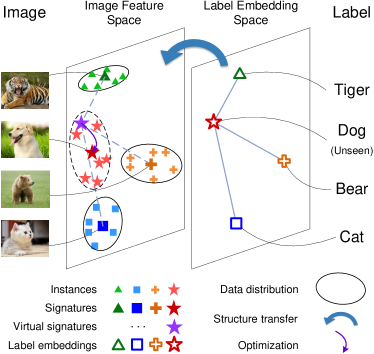
Figure 1: Illustration of the proposed method. The manifold structure (the straight lines) in the label embedding space is transferred to the image feature space for synthesizing the virtual signature (the purple star) of an unseen class. The purple arrow points to a refined signature, which demonstrates that the synthesized virtual signature is optimized after running the Expectation-Maximization algorithm so that unseen data are assigned to labels according to the data distribution.

The recent success of deep learning heavily relies on a large amount of labeled training data. For some classes, e.g., rare wildlife and unusual diseases, it is expensive even impossible to collect thousands of samples. Traditional supervised learning frameworks cannot work well in this situation. Zero-shot learning (ZSL) that aims to recognize instances of an unseen class is considered to be a promising solution.

In ZSL, data are (datum, label) pairs and these data pairs are split into labeled seen classes (source domain) and unlabeled unseen classes (target domain where labels are missing). The seen classes and unseen classes are disjointed. Therefore, “auxiliary information” is introduced to enable knowledge transfer from seen classes to unseen ones so that given a datum from the unseen classes, its label can be predicted. Often used auxiliary information includes attributesLampert et al. (2014), textual descriptionLei Ba et al. (2015) and word vectors of labelsSocher et al. (2013)), etc. In most practice, labels are embedded in “label embedding space”. Data (e.g., images) are embedded in (e.g., image) feature space (using hand-craft or deep learning feature extractors). In the following of this paper, we introduce ZSL in the context of image recognition.

One popular type of ZSL is implemented in an inductive way, i.e. models are trained on seen classes then applied to unseen classes directly. Usually, inductive ZSL includes three steps: i) embedding images and labels in the image feature space and label embedding space respectively; ii) learning the mapping function from the image feature space to the label embedding space (F$\rightarrow$E); iii) mapping an unseen image to the label embedding space using the learned mapping function and predicting its label. In this way, ZSL is posed as a missing label problem. Many existing methods of this type (e.g., Socher et al. (2013)Al-Halah et al. (2016)Qiao et al. (2016)) assume a global linear mapping F$\rightarrow$E between the two spaces. Romera-Paredes and Torr (2015) present a very simple ZSL approach using this assumption, and extend the approach to a kernel version. However, the global linear mapping assumption can be over-simplified. Wang et al. (2016) propose to utilize local relational knowledge to synthesize virtual unseen image data so as to simulate the manifold structure of unseen classes, but then back to the global linear assumption to learn the mapping F$\rightarrow$E using both the seen data and synthesised unseen data. We observe that the synthesized manifold structure of unseen classes is not accurate, in addition, back to the global linear mapping assumption further damage the ZSL performance. Hence adaptation should be introduced to adjust the synthesized manifold structure according to the real unseen data.

Accordingly, many transductive ZSL approaches are proposed for alleviating the domain adaptation problemFu et al. (2015). In transductive ZSL, (unlabeled) real unseen data are utilized for refining the trained model, e.g., the label embedding space and mapping function F$\rightarrow$E. Li et al. (2015) propose a semi-supervised method to learn new label embeddings using prior knowledge of the original ones. In Kodirov et al. (2015), a dictionary for the target domain (unseen classes) is learned using regularised sparse coding, and the dictionary learned on the source domain (seen classes) serves as the regularizer. In Zhang and Saligrama (2016b), a structured prediction approach is proposed. Several clusters on unseen data are generated using K-means, then a bipartite graph matching between these clusters and labels is optimized based on the learned similarity matrix on seen data.

Most aforementioned methods aim at learning a potentially complex mapping from F$\rightarrow$E. Under circumstances such as the number of classes is large and there exists polysemy in text labels, such many-to-one “clean mapping” can be hard to learn. In this paper, we study a novel transductive zero-shot learning method (shown in Figure.1), which transfers the manifold structure in the label embedding space to the image feature space (E$\rightarrow$F), and adapts the transferred structure according to the underlying data distribution of both seen and unseen data in the image feature space. As the proposed method associates data to the label, we categorize it as a missing data method in contrast to the conventional missing label methods.

Our method is based on two assumptions, i) data of each class in the image feature space follow a Gaussian distribution, ii) the local manifold structure of label embeddings are approximate to that of “the signatures” in the image feature space. In previous works, the signatureRomera-Paredes and Torr (2015) or prototypeFu et al. (2015) is used to denote the authentic distribution of data of each class in the label embedding space. While, in our reverse mapping, we use the “signature” to denote the authentic distribution of data of each class in the image feature space. Data distributions are modeled by Gaussians, and “the signatures” are defined as the model parameters of Gaussians. Our method consists of three main steps:

i) The signature of each seen class is estimated in the image feature space.

ii) The manifold structure is estimated in the labeling embedding space, and is transferred to the image feature space so as to synthesize virtual signatures of the unseen classes in the image feature space.

iii) The virtual signatures are refined, at the same time, each unseen instance is associated to an unseen label (label prediction) by the Expectation-Maximization (EM) algorithm.

Experiments show that the proposed method achieves the state-of-the-art performance on two popular datasets, namely, the Animals with Attributes and the Caltech-UCSD Birds-200-2011. It outperforms the runner-up by nearly 5% and 10% on default and random splits, respectively.

2 The Proposed Method

$N^{s}$ seen classes data are denoted as $(\bm{X}^{s},\bm{Y}^{s})=\{(\bm{x}^{s}_{1},{y}^{s}_{1}),...,(\bm{x}^{s}_{N^{s}},{y}^{s}_{N^{s}})\}$, and $N^{u}$ unseen classes data are denoted as $(\bm{X}^{u},\bm{Y}^{u})=\{(\bm{x}^{u}_{1},{y}^{u}_{1}),...,(\bm{x}^{u}_{N^{u}},{y}^{u}_{N^{u}})\}$. Each datum $\bm{x}^{s}_{i}$ or $\bm{x}^{u}_{i}$ $\in\Re^{d\times 1}$ is a $d$-dimensional feature vector in the image feature space. ${y}^{s}_{i}$ or ${y}^{u}_{i}$ denotes the labels. The label sets of the seen and unseen classes are disjointed, i.e. $\bm{Y}^{s}\cap\bm{Y}^{u}=\emptyset$. The “auxiliary information” from corpus (e.g. word vectors) or/and annotations (e.g. attributes) are label embeddings denoted as $\bm{E}^{s}=\{\bm{e}^{s}_{1},...,\bm{e}^{s}_{K^{s}}\}$ and $\bm{E}^{u}=\{\bm{e}^{u}_{1},...,\bm{e}^{u}_{K^{u}}\}$ for seen and unseen classes respectively. $\bm{e}^{s}_{i}$ and $\bm{e}^{u}_{i}$ $\in\Re^{d^{\prime}\times 1}$. Using the seen data pairs $(\bm{x}^{s}_{i},{y}^{s}_{i})$, ZSL aims to predict labels ${y}^{u}_{i}$ for each unseen instance $\bm{x}^{u}_{i}$ by leveraging the “auxiliary information” $\bm{E}^{s}$ and $\bm{E}^{u}$ for knowledge transfer.

2.1 Estimation of Seen Classes Signatures

By dimensionality reduction (using t-SNEMaaten and Hinton (2008)), it is observed that data of each class form a tight cluster (shown in Figure.2) in the image feature space. Hence, we assume that

Assumption 1

Data of each class follow a Gaussian distribution $\bm{X}\sim{\cal N}(\bm{\mu},\bm{\Sigma})$ in the image feature space.

It is worth noting that in the literature people used Nearest-Neighbor classifiers to assign labels to unseen data, e.g., Palatucci et al. (2009) Fu and Sigal (2016), the underlying assumption is that the distribution of the data is isotropic Gaussian. Here we estimate the parameters of the Gaussians.

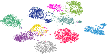
Figure 2: Visualization of the default 10 unseen classes in Animals with Attributes dataset using t-SNE. Instances within each class form a tight cluster.

2.1.1 Estimation of the Signatures

Similar to Romera-Paredes and Torr (2015), we use “signature”, denoted as $\bm{S}=\{\bm{s}_{1},...,\bm{s}_{K}\}$, to represent the data distribution of each class in the image feature space. The signature is the sufficient statistics of the data, and using it the distribution of the data can be recovered. Here, for a Gaussian model, the signature is $\bm{s}_{k}=(\bm{\mu}_{k},\bm{\Sigma}_{k})$, i.e. the mean and covariance. As the labels of seen classes data are provided, we can estimate signatures of seen classes directly, denoted as $\bm{S}^{s}$.

2.2 Synthesis of Virtual Signatures

One of the key challenges in ZSL is to explore the relationship between the image feature space and the label embedding space. The label embedding is either pre-designed (e.g. by the annotated attribute vectors) or pre-trained on a large corpus (e.g. by word vectors). Although there may not be an accurate global linear mapping from the image feature space to the label embedding space, local manifold structures may be similar of the two. In this paper we focus on exploiting the local manifold structure rather than the global one. Hence we assume that

Assumption 2

The local manifold structure of label embeddings is approximate to that of the signatures in the image feature space and can be transferred for synthesizing the virtual signatures of the unseen classes.

This is formulated as

$$\bm{E}^{u}=R\left(\bm{E}^{s}\right)\Rightarrow\widehat{\bm{S}^{u}}=R\left(\bm{S}^{s}\right),$$ (1)

where $\widehat{\bm{S}^{u}}=\{\widehat{\bm{s}^{u}_{1}},...,\widehat{\bm{s}^{u}_{K^{u}}}\}$ denotes the synthesized virtual signatures of the unseen classes. There are many choices of the synthesis function $R(\cdot)$ that can approximate the manifold structure of the label embeddings, such as Sparse Coding, K-Nearest Neighbors and so on.

In the literature, many works assume the two spaces observe a global linear transformation so that the structure of the image features can be transferred to the label embeddings via a global linear mapping, e.g., Al-Halah et al. (2016)Qiao et al. (2016). We observe that such an assumption is over-simplified. There are works assuming that a global non-linear mapping may exist between the two spacesRomera-Paredes and Torr (2015), e.g., using kernel methods. However, it is prone to get overfitting on the seen data and obtain bad performance on the unseen data. In contrast, our manifold preserving assumption works well empirically in the experiments.

2.2.1 Synthesis via Sparse Coding

We choose Sparse CodingOlshausen and Field (1997) (inspired by Wang et al. (2016)) to approximate the manifold structures of the image features and label embeddings. In our implementation, label embeddings of the seen classes serve as the dictionary. Then we compute the sparse linear reconstruction coefficients of the bases for unseen label embeddings. According to the Sparse Coding theory, we minimize the following loss function to obtain the coefficients $\bm{\alpha}$.

$$\min_{\bm{\alpha}}\left\|\bm{e}^{u}_{k}-\bm{E}^{s}\bm{\alpha}\right\|^{2}+\lambda|\bm{\alpha}|_{1},$$ (2)

where $\bm{\alpha}={[\alpha_{1},...,\alpha_{K^{s}}]}^{T}$. This loss function is convex and easy to optimize.

Then, we transfer such local structure from the label embedding space to the image feature space and synthesize the virtual signature of each unseen class using the same set of coefficients, i.e. $\widehat{\bm{s}^{u}_{k}}=\bm{S}^{s}\bm{\alpha}$, where the components in $\bm{E}^{s}$ and $\bm{S}^{s}$ correspond to each other. This transferring is valid because that the distribution of an unseen class in the image space is assumed to be a Gaussian and the components either in $\bm{E}^{s}$ or $\bm{S}^{s}$ are assumed to be independent.

After synthesizing all unseen signatures (say $K^{u}$ of them), the distribution of the unseen instances $\{\bm{x}^{u}_{n}\}$ in the image feature space is a Gaussian Mixture Model (GMM),

$$p\left({\bm{x}^{u}_{n}}\right)=\sum\limits_{k=1}^{K^{u}}{{\pi_{k}}{\cal N}\left({\bm{x}^{u}_{n}|{\bm{\mu}_{k}},{\bm{\Sigma}_{k}}}\right)}$$ (3)

$\pi_{k}$ denotes the $k$th mixing coefficient and its initial value is assumed to be $1/K^{u}$. The initial value of $(\bm{\mu}_{k},\bm{\Sigma}_{k})=\widehat{\bm{s}^{u}_{k}}$. $\bm{x}^{u}_{n}$ denotes the $n$th image in $\bm{X}^{u}$.

The synthesized virtual signatures approximate the distribution of the unseen data in the image feature space. However, they may not be accurate. Next, we optimize/refine the signatures, at the same time, associate each unseen image to an unseen label. This is the reason we pose our ZSL as a missing data problem.

2.3 Solving the Missing Data Problem

We impute unseen image labels and update the GMM parameters using the Expectation-Maximization (EM) algorithm.

The objective function is defined as the log of the likelihood function,

$$\ln{p\left({{\bm{X}^{u}}|{\bm{\pi},\bm{\mu}},\bm{\Sigma}}\right)}=\sum_{n=1}^{N^{u}}{\ln{}}\sum\limits_{k=1}^{K^{u}}{{\pi_{k}}{\cal N}\left({{\bm{x}^{u}_{n}}|{\bm{\mu}_{k}},{\bm{\Sigma}_{k}}}\right)}$$ (4)

In the Expectation step, the conditional probability of the latent variable $y^{u}_{n}=k$ given $\bm{x}^{u}_{n}$ under the current parameter is

$$p(y^{u}_{n}=k|\bm{x}^{u}_{n})=\frac{{\pi_{k}}{\cal N}\left({{\bm{x}^{u}_{n}}|{\bm{\mu}_{k}},{\bm{\Sigma}_{k}}}\right)}{\sum_{j=1}^{K^{u}}{{\pi_{j}}{\cal N}\left({{\bm{x}^{u}_{n}}|{\bm{\mu}_{j}},{\bm{\Sigma}_{j}}}\right)}}.$$ (5)

This is the posterior probability of an unseen image $\bm{x}^{u}_{n}$ belonging to label $k$.

In the Maximization step, the model updates the parameters using the posterior probability.

$$\bm{\mu}_{k}^{new}=\frac{1}{N^{u}}\sum_{n=1}^{N^{u}}{p(y^{u}_{n}=k|\bm{x}^{u}_{n})\bm{x}^{u}_{n}}$$ (6)

$$\bm{\Sigma}_{k}^{new}=\frac{1}{N^{u}}\sum_{n=1}^{N^{u}}{p(y^{u}_{n}=k|\bm{x}^{u}_{n})(\bm{x}^{u}_{n}-\bm{\mu}_{k}^{new})^{T}(\bm{x}^{u}_{n}-\bm{\mu}_{k}^{new})}$$ (7)

$$\pi^{new}_{k}=\frac{N^{u}_{k}}{N^{u}}$$ (8)

where

$$N^{u}_{k}=\sum_{n=1}^{N^{u}}{p(y^{u}_{n}=k|\bm{x}^{u}_{n})}$$ (9)

$K^{u}$ and $N^{u}$ denote the number of all unseen classes and instances respectively. We iterate the E-step and M-step until convergence. After the convergence, the parameters of the data distribution are refined and the unseen instances are assigned with labels.

2.3.1 Regularization

During the EM process when estimating the GMM, each covariance matrix $\bm{\Sigma}_{k}$ should be nonsingular, i.e. invertible. For a reliable computation, empirically, the number of data in each class $N_{k}$ should be greater than the square of feature dimension, i.e. $\forall_{k},N_{k}\geq\lambda d^{2},s.t.\;\lambda\geq 1$. $\lambda$ is a coefficient. However, this may not be satisfied in some situations when feature dimension is high but only a small number of data are provided per class.

We employ two tricks to solve this problem, namely, dimensionality reduction and regularization of $\bm{\Sigma}_{k}$. For dimensionality reduction, we choose to use linear dimension reduction methods, e.g. principal components analysis (PCA), to reduce the image feature representation to $d$ dimensional, which is much smaller than the original one.

If we only choose to stabilize the computation by reducing the image feature dimension, the label prediction accuracy will degrade quickly. Hence, we also resort to another solution, i.e., regularizing $\bm{\Sigma}_{k}$. Here, we present two regularization methods of $\bm{\Sigma}_{k}$, namely, diagonal $\bm{\Sigma}_{k}$, $s.t.\;N_{k}\geq\lambda d$ and unit $\bm{\Sigma}_{k}$, $s.t.\;N_{k}\geq 1$. Diagonal $\bm{\Sigma}_{k}$ means that $\bm{\Sigma}_{k}$ is assumed to be a diagonal matrix. Unit $\bm{\Sigma}_{k}$ means that $\bm{\Sigma}_{k}$ is an identity matrix. These two regularization methods simplify $\bm{\Sigma}_{k}$ in an increasing order. We choose to use a simpler one if the number of the data is smaller.

3 Experiments

3.1 Datasets & Settings

In this section, we evaluate the proposed method by conducting experiments on two popular datasets, i.e., the Animals with Attributes (AwA) Lampert et al. (2009) and the Caltech-UCSD Birds-200-2011 (CUB) Wah et al. (2011).

AwA contains 50 classes and 85 manual attributes (both binary and continuous). The average number of the images of each class is 610, and the minimum number is 92. Ten classes serve as the unseen classes and the remaining forty are utilized as the seen classes. Lampert et al. (2014) provided a fixed default split, which is used as the default split in many works.

CUB is a fine-grained image dataset which contains 200 species of birds annotated with 312 binary attributes. The mean and minimum numbers of bird images of each class are 60 and 41 respectively. Commonly, 50 species are chosen as the unseen classes, and the rest are the seen classes. The fixed default split used in this paper follows that in Wang et al. (2016).

For AwA, we use i) 4096-dimensional VGG features (VGG-fc7) provided along with the dataset, ii) 1024-dimensional GoogLeNet features, iii) 1000-dimensional ResNet features. For CUB, we use iv) 1024-dimensional GoogLeNet features, v) 1000-dimensional VGG features (VGG-fc8) and vi) 2048-dimensional ResNet features extracted on the Pooling-5 layer. ii, iii, iv, v) are provided by Wang et al. (2016). The label embeddings (attributes and word vectors) used in this paper are the same as Wang et al. (2016).

Most previous works presented their experimental results using a fixed default split or a few random splits of the seen/unseen classes on different datasets. We argue that the evaluation based on the fixed default split or only a few random splits may not be comprehensive/stable enough, especially on small-scale datasets. For a fair comparison, we evaluate our method on both “many random splits” and the fixed default split. “Many random splits” means that we conduct all experiments with 300 random splits.

3.2 Analysis of Data Distribution

First, we examine if Assumption 1 is a reasonable assumption, i.e. the data of each class approximately subject to a Gaussian distribution in the image feature space. The idea is to show that under this assumption the upper bound of the proposed ZSL performance exceeds that of the state-of-the-art methods by a considerable margin.

To obtain the upper bound performance of the proposed method under Assumption 1, we conduct a upper-bound experiment, in which the labels of all data (both seen and unseen) are given. Hence, we can estimate the Gaussian distribution for each class according to the data labels. Then the label of each datum is predicted as the one with the maximum likelihood of the Gaussians/classes. The mean classification accuracy consequently can be computed.

Table.1 shows the upper-bound classification performances of the proposed method based on Assumption 1 in different image feature spaces. All-50 means that we estimate Gaussian distributions on all 50 classes of AwA and report the overall classification accuracy. Unseen-10 means we estimate Gaussians on 10 randomly selected classes as unseen classes and the classification accuracy is the average over 300 such random trials. All-200 and Unseen-50 have the similar meanings for CUB dataset.

For all classes of AwA, modeling data with Gaussian achieves 84.55% classification accuracy in VGG-fc7 feature space. For all classes of CUB, the classification accuracy is 73.81% in GoogLeNet+ResNet feature space.

The experimental upper bound performance under Assumption 1 on AwA Unseen-10 and CUB Unseen-50 are 92.10% and 85.03% using VGG-fc7 and GoogLeNet + ResNet features respectively. According to Table.3, the proposed upper-bound performance is much larger than the corresponding state-of-the-art performance – 68.05% (RKT) and 61.69% (RKT) on AwA and CUB respectively. Therefore, the Gaussian assumption of the distribution of data is reasonably good currently when comparing the proposed method with the other state-of-the-arts.

It is worth noting that it is reasonable for CUB to have a lower upper-bound than that of AwA, as CUB is a fine-grained bird species dataset, hence the classification is harder.

	Image Feature	Setting	Acc. %
AwA	VGG-fc7	All-50	84.55
		Unseen-10	92.10
	GoogLeNet	All-50	81.44
	ResNet	All-50	73.51
CUB	GoogLeNet + ResNet	All-200	73.81
		Unseen-50	85.03
	GoogLeNet	All-200	67.48
	GoogLeNet + VGG-fc8	All-200	60.43

Table 1: Analysis of data distribution assumption. All-50 and Unseen-10 means that we estimate the GMM on all 50 classes and random 10 unseen classes of AwA respectively. All-200 and Unseen-50 have the similar meanings for CUB. The high classification accuracies explain that Assumption 1 is effective in different feature spaces and datasets.

3.3 Effectiveness of Virtual Signatures

To justify Assumption 2, we evaluate the classification performance using synthesized virtual signatures directly. This strategy can be viewed as inductive ZSL. We run 300 random trials on AwA and CUB respectively. Features extracted from VGG-fc7 (4096-dim) for AwA and GoogLeNet+ResNet (3072-dim) for CUB are utilized. We use the same label embeddings as those in Wang et al. (2016). According to our analysis in Sec.2.3.1, the image feature dimension is reduced to 80-dim on AwA. Because the minimum number of images of each class is 92. We also reduce the feature dimension of CUB data to 400-dim for speeding up the computation. Three types of label embedding are tested, namely, attributes(A), word vectors(W) and attributes with word vectors(A+W). Results using different settings are shown in Table.2.

As shown in Table.2, the classification accuracies using synthesized signatures without EM step are 72.11% on AwA and 59.94% on CUB (using A+W label embeddings), which is comparable to the sate-of-the-art (see Table.3 and Table.4). These results show that the synthesized signatures are reasonably good and so is Assumption 2.

We find that the performance using word vectors (60.99%) as label embedding is better than that using attributes (58.73%) on AwA. However, this phenomenon reverses on CUB (i.e. 47.31% using word vectors and 56.21% using attributes). A possible reason is that the general training corpus for the word vector model is not specific to fine-grained bird species. So word vectors of fine-grained species names do not work well as those of the general animal names.

3.4 Evaluation of the EM Optimization

Here, we evaluate the gain brought by the EM optimization (shown in Table.2). All data (features, label embeddings, random splits) are consistent with those in the previous subsection. GMM with diagonal $\bm{\Sigma}_{k}$ (GMM-EM-Diagonal) and unit $\bm{\Sigma}_{k}$ (GMM-EM-Unit) are tested. For AwA, GMM-EM-Unit brings about 17% improvement of classification accuracy using the three label embeddings on average. Using GMM-EM-Diagonal increases nearly 1% classification accuracy over the GMM-EM-Unit. For CUB, nearly 6% improvement is brought by using GMM-EM-Unit. The experiment using GMM-EM-Diagonal on CUB is not reported due to the lack of training data (about 60 data in each class, which is explained in Sec.2.3.1). These results show that the EM optimization improves classification performances in different settings.

We also implement a baseline algorithm to show the effectiveness of using synthesized signatures as the initialization of the EM optimization as shown in Table.2. In Baseline-Random-Init.-EM, we randomly pick a set of unseen datapoints to initialize the mean of the GMM components, then execute the EM optimization. The resulted classification accuracies are 9.46% on AwA and 2.00% on CUB respectively, which are at chance level.

	Label Embedding	Acc. % of Syn.-Sig	Acc. % of GMM-EM-Unit	Acc. % of GMM-EM-Diagonal	Baseline Random-Init.-EM
AwA	A	58.73	82.44	83.39	9.46
	W	60.99	75.31	76.31
	A+W	72.11	86.39	87.38
CUB	A	56.21	61.27	-	2.00
	W	47.31	55.62
	A+W	59.94	63.37

Table 2: Evaluate the synthesized virtual signatures with and without the EM optimization algorithm under the 300 random split setting. Syn.-Sig. denotes classification directly using the synthesized virtual signatures. GMM-EM-Diagonal and GMM-EM-Unit are two regularization methods that use diagonal $\bf{\Sigma}_{k}$ and unit $\bf{\Sigma}_{k}$ in the EM algorithm to estimate the GMM. Using GMM-EM with unit $\bm{\Sigma}_{k}$ brings about 17% and 6% improvement on AwA and CUB respectively. On AwA, using GMM-EM with diagonal $\bm{\Sigma}_{k}$ increases nearly 1% classification accuracy over the one using the unit $\bm{\Sigma}_{k}$. The last column shows that if we initialize the GMM component using random datapoints, the classification accuracy is at chance level.

3.5 Comparison to the State-of-the-Art

First, we compare our method to two popular methods, namely ESZSL Romera-Paredes and Torr (2015) and RKT Wang et al. (2016), using provided codes. We repeat these experiments using the same setting (including image features, label embeddings, the default split and 300 random splits ) as the aforementioned in Sec.3.3. Although we have to reduce image feature dimensions in our method, we use the original image features for other methods.

From Table.3, it can be seen that on AwA the average classification accuracy of our method is 87.38%, which outperforms that of the runner-up (RKT) 68.05% by 19.33% on the random splits. On CUB, the performance of our method is 63.37%, which also exceeds that of the runner-up (RKT) 61.69% by 1.68% on the random splits. This superiority is also observed on the default split setting on two datasets. We use the same set of model parameters for both the default and random split settings, rather than using different parameters on different settings. The inductive version of our method (Ours_I) achieves comparable results on the two split settings on two datasets.

From Figure.3 we find that the variance of the random split classification accuracies is large for all the three methods on AwA. By contrast, the classification accuracies of the default split (marked as stars in the figure) are all in good positions in the performance bars. This supports our argument that the experiments on large number of random splits are necessary for reliable results and comparison.

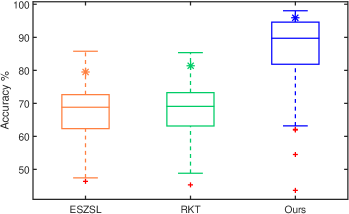
Figure 3: Box plots of results of different methods on AwA. The three box plots illustrate the classification accuracy statistics of the ESZSL, RKT and our method on 300 random splits. On each box, the central mark is the median, the edges of the box are the 25th and 75th percentiles. It is shown that the variance of random split results is large. The stars represent results of the three methods on the default split.

Table 3: Comparison to popular methods using the same setting. Ours_I is our method using the synthesized virtual signatures directly for classification without the EM optimization.

	Method	Image Feature	Accuracy %
			Default	Random
AwA	ESZSL	VGG-fc7	79.53	67.75
	RKT		81.41	68.05
	Ours_I		82.07	72.11
	Ours		95.99	87.38
CUB	ESZSL	GoogLeNet + ResNet	51.90	57.62
	RKT		55.59	61.69
	Ours_I		57.31	59.94
	Ours		60.24	63.37

We also compare with the results reported in recent papers, namely DAP/IAP Lampert et al. (2014), ESZSL Romera-Paredes and Torr (2015), SJE Akata et al. (2015), SC_struct Changpinyo et al. (2016), SS-Voc Fu and Sigal (2016), JLSE Zhang and Saligrama (2016a), Mul-Cue Akata et al. (2016), TMV-HLP Fu et al. (2014), RKT Wang et al. (2016), SP-ZSR Zhang and Saligrama (2016b) and LatEm Xian et al. (2016). From Table.4, it can be seen that our method achieves the best performance on the both datasets.

From Table.4, it can be seen that on AwA our method achieves the best accuracy on the default split, i.e. 95.99%, which is 3.91% improvement compared to the runner-up method, i.e. 92.08% of SP-ZSR. There are few works, namely LatEm, SC_struct and DAP/IAP, evaluated on random splits, but only on a few random trials. We evaluate our method on 300 random trials and achieve 87.38% classification accuracy on AwA. Our result is almost 11.28% higher than that of the runner-up, LatEm.

From Table.4, it can be seen that the average performance on CUB is not as good as that on AwA. This is also observed in the previous experiments. Our method achieves 60.24% classification accuracy on the default split, which outperforms the runner-up (SP-ZSR) by 4.90%. Notice that the classification accuracy of 56.5% achieved by Mul-Cue requires manual annotation for the bird part locations of the test images. So, it is not fair to compare with this result directly. Our method receives 63.37% mean accuracy on the 300 random splits. This result is 8.67% higher than the runner-up (SC_struct). Overall, our method achieves nearly 5% and 10% improvement on the default and random splits respectively compared to reported results on the both datasets.

	Methods	Split	AwA	CUB
Default	DAP/IAP		41.4/42.2	-
	ESZSL	Default	49.30	-
	SJE		66.7	50.1
	SC_struct		72.9	-
	SS-Voc		78.3	-
	JLSE		80.46	42.11
	Mul-Cue		-	56.5*
				43.3
	TMV-HLP		80.5	47.9
	RKT		82.43	46.24
	SP-ZSR		92.08	55.34
	Ours		95.99	60.24
Random	DAP/IAP	5 trials	37.1/34.1	-
	LatEm	1 default + 4 trials	76.1	47.4
	SC_struct	4 trials	-	54.7
	Ours	300 trials	87.38	63.37

Table 4: Comparison to the state-of-the-art. * means extra information is used. On AwA, our method outperforms the runner-ups by 3.91% and 11.28% on the default and random splits respectively. On CUB, our method outperforms the runner-ups by 4.90% and 8.67% on the default and random splits respectively.

4 Conclusion

In this paper, we propose a transductive zero-shot learning method based on the estimation of data distribution by posing ZSL as a missing data problem. Different from others, we focus on exploiting the local manifold structure in two spaces rather than the global mapping. Testing data are classified in the image feature space based on the estimated data distribution. Experiments show that the proposed method outperforms the state-of-the-art methods on two popular datasets.

References

- Akata et al. [2015] Zeynep Akata, Scott Reed, Daniel Walter, Honglak Lee, and Bernt Schiele. Evaluation of output embeddings for fine-grained image classification. In Proceedings of the IEEE Conference on Computer Vision and Pattern Recognition, pages 2927–2936, 2015.
- Akata et al. [2016] Zeynep Akata, Mateusz Malinowski, Mario Fritz, and Bernt Schiele. Multi-cue zero-shot learning with strong supervision. In Proceedings of the IEEE Conference on Computer Vision and Pattern Recognition, pages 59–68, 2016.
- Al-Halah et al. [2016] Ziad Al-Halah, Makarand Tapaswi, and Rainer Stiefelhagen. Recovering the missing link: Predicting class-attribute associations for unsupervised zero-shot learning. In Proceedings of the IEEE Conference on Computer Vision and Pattern Recognition, pages 5975–5984, 2016.
- Changpinyo et al. [2016] Soravit Changpinyo, Wei-Lun Chao, Boqing Gong, and Fei Sha. Synthesized classifiers for zero-shot learning. In Proceedings of the IEEE Conference on Computer Vision and Pattern Recognition, pages 5327–5336, 2016.
- Fu and Sigal [2016] Yanwei Fu and Leonid Sigal. Semi-supervised vocabulary-informed learning. In Proceedings of the IEEE Conference on Computer Vision and Pattern Recognition, pages 5337–5346, 2016.
- Fu et al. [2014] Yanwei Fu, Timothy M Hospedales, Tao Xiang, Zhenyong Fu, and Shaogang Gong. Transductive multi-view embedding for zero-shot recognition and annotation. In European Conference on Computer Vision, pages 584–599. Springer, 2014.
- Fu et al. [2015] Yanwei Fu, Timothy M Hospedales, Tao Xiang, and Shaogang Gong. Transductive multi-view zero-shot learning. IEEE transactions on pattern analysis and machine intelligence, 37(11):2332–2345, 2015.
- Kodirov et al. [2015] Elyor Kodirov, Tao Xiang, Zhenyong Fu, and Shaogang Gong. Unsupervised domain adaptation for zero-shot learning. In Proceedings of the IEEE International Conference on Computer Vision, pages 2452–2460, 2015.
- Lampert et al. [2009] Christoph H Lampert, Hannes Nickisch, and Stefan Harmeling. Learning to detect unseen object classes by between-class attribute transfer. In Computer Vision and Pattern Recognition, 2009. CVPR 2009. IEEE Conference on, pages 951–958. IEEE, 2009.
- Lampert et al. [2014] Christoph H Lampert, Hannes Nickisch, and Stefan Harmeling. Attribute-based classification for zero-shot visual object categorization. IEEE Transactions on Pattern Analysis and Machine Intelligence, 36(3):453–465, 2014.
- Lei Ba et al. [2015] Jimmy Lei Ba, Kevin Swersky, Sanja Fidler, et al. Predicting deep zero-shot convolutional neural networks using textual descriptions. In Proceedings of the IEEE International Conference on Computer Vision, pages 4247–4255, 2015.
- Li et al. [2015] Xin Li, Yuhong Guo, and Dale Schuurmans. Semi-supervised zero-shot classification with label representation learning. In Proceedings of the IEEE International Conference on Computer Vision, pages 4211–4219, 2015.
- Maaten and Hinton [2008] Laurens van der Maaten and Geoffrey Hinton. Visualizing data using t-sne. Journal of Machine Learning Research, 9(Nov):2579–2605, 2008.
- Olshausen and Field [1997] Bruno A Olshausen and David J Field. Sparse coding with an overcomplete basis set: A strategy employed by v1? Vision research, 37(23):3311–3325, 1997.
- Palatucci et al. [2009] Mark Palatucci, Dean Pomerleau, Geoffrey E Hinton, and Tom M Mitchell. Zero-shot learning with semantic output codes. In Advances in neural information processing systems, pages 1410–1418, 2009.
- Qiao et al. [2016] Ruizhi Qiao, Lingqiao Liu, Chunhua Shen, and Anton van den Hengel. Less is more: zero-shot learning from online textual documents with noise suppression. In Proceedings of the IEEE Conference on Computer Vision and Pattern Recognition, pages 2249–2257, 2016.
- Romera-Paredes and Torr [2015] Bernardino Romera-Paredes and PHS Torr. An embarrassingly simple approach to zero-shot learning. In Proceedings of The 32nd International Conference on Machine Learning, pages 2152–2161, 2015.
- Socher et al. [2013] Richard Socher, Milind Ganjoo, Christopher D Manning, and Andrew Ng. Zero-shot learning through cross-modal transfer. In Advances in neural information processing systems, pages 935–943, 2013.
- Wah et al. [2011] C. Wah, S. Branson, P. Welinder, P. Perona, and S. Belongie. The Caltech-UCSD Birds-200-2011 Dataset. Technical Report CNS-TR-2011-001, California Institute of Technology, 2011.
- Wang et al. [2016] Donghui Wang, Yanan Li, Yuetan Lin, and Yueting Zhuang. Relational knowledge transfer for zero-shot learning. In Thirtieth AAAI Conference on Artificial Intelligence, 2016.
- Xian et al. [2016] Yongqin Xian, Zeynep Akata, Gaurav Sharma, Quynh Nguyen, Matthias Hein, and Bernt Schiele. Latent embeddings for zero-shot classification. In Proceedings of the IEEE Conference on Computer Vision and Pattern Recognition, pages 69–77, 2016.
- Zhang and Saligrama [2016a] Ziming Zhang and Venkatesh Saligrama. Zero-shot learning via joint latent similarity embedding. In Proceedings of the IEEE Conference on Computer Vision and Pattern Recognition, pages 6034–6042, 2016.
- Zhang and Saligrama [2016b] Ziming Zhang and Venkatesh Saligrama. Zero-shot recognition via structured prediction. In European Conference on Computer Vision, pages 533–548. Springer, 2016.