Gradient Descent Finds the Cubic-Regularized Non-Convex Newton Step

Abstract

We consider the minimization of non-convex quadratic forms regularized by a cubic term, which exhibit multiple saddle points and poor local minima. Nonetheless, we prove that, under mild assumptions, gradient descent approximates the global minimum to within $\varepsilon$ accuracy in $O(\varepsilon^{-1}\log(1/\varepsilon))$ steps for large $\varepsilon$ and $O(\log(1/\varepsilon))$ steps for small $\varepsilon$ (compared to a condition number we define), with at most logarithmic dependence on the problem dimension. When we use gradient descent to approximate the cubic-regularized Newton step, our result implies a rate of convergence to second-order stationary points of general smooth non-convex functions.

1 Introduction

We study the optimization problem

$$\mathop{\rm minimize}_{x\in\mathbb{R}^{d}}~{}f\left(x\right)\triangleq\frac{1}{2}x^{T}Ax+b^{T}x+\frac{\rho}{3}\left\|x\right\|^{3},$$ (1)

where the matrix $A$ is symmetric and possibly indefinite. The problem (1) arises in Newton’s method with cubic regularization, for (approximately) minimizing a general smooth function $g$. The method consists of the iterative procedure

$$y_{t+1}=y_{t}+\mathop{\rm argmin}_{x\in\mathbb{R}^{d}}\left\{\nabla g(y_{t})^{T}x+\frac{1}{2}x^{T}\nabla^{2}g(y_{t})x+\frac{\rho_{t}}{3}\left\|{x}\right\|^{3}\right\},$$ (2)

where every iteration requires solution of a problem of the form (1) and choice of the parameter $\rho_{t}$. Griewank [15] first proposed the scheme (2) (in a more general setting), and then Nesterov and Polyak [25] and Weiser et al. [33] independently rediscovered it. Cubic regularization methods, as well as the closely related trust-region methods, are among the most practically successful and theoretically sound approaches to non-convex optimization [9, 25, 7]. Indeed, Nesterov and Polyak [25] establish that $O(\epsilon^{-3/2})$ iterations of the form (2) suffice to find an $\epsilon$-second-order-stationary point of $g$, meaning a point $y_{\epsilon}$ such that $\left\|{\nabla g(y_{\epsilon})}\right\|\leq\epsilon$ and $\lambda_{\min}(\nabla^{2}g(y_{\epsilon}))\gtrsim-\sqrt{\epsilon}$. However, this complexity guarantee does not account for the computational cost of solving subproblems of the form (1).

In this work, we study what is perhaps the simplest algorithm for approximately solving the problem (1): gradient descent. Each iteration of gradient descent consists of the transformation $x\mapsto x-\eta\nabla f(x)=x-\eta(Ax+b+\rho\left\|{x}\right\|x)$ for a step-size $\eta\in\mathbb{R}$. Thus, the computational cost of a gradient descent iteration is essentially that of multiplying the matrix $A$ with a vector. Iterative methods requiring only matrix-vector products are called matrix-free, and are especially appealing in the setting when $d$ is large and $A$ has structure, such as sparsity (cf. [32]), which enables efficient computation of $Ax$. Notably, when $A$ is a Hessian as in (2), it is often possible to compute $Ax$ in time linear in $d$ [27, 29], comparable to the time to evaluate a gradient.

We do not claim that gradient descent is the most efficient method for solving problem (1). Indeed, popular matrix-free Krylov subspace solvers [7] provide faster convergence by definition, as the first $k$ iterates of gradient descent lie in the Krylov subspace of order $k$, $\mathrm{span}\{b,Ab,\ldots,A^{k-1}b\}$. Moreover, two-term recursions such as the heavy-ball method [28] and Nesterov’s accelerated gradient descent [22] outperform gradient descent in convex problems, with results extending to several non-convex scenarios [5]. Yet we believe gradient descent—as a workhorse for numerous large-scale problems—is a valuable object of study, for the following reasons.

1. By proving concrete upper bounds on the number of gradient steps required to achieve an $\varepsilon$-accurate solution to the problem (1), we obtain a benchmark for more sophisticated algorithms, such as Krylov subspace methods, and providing dimension-independent guarantees on the number of matrix-vector products such methods require to solve (1) to $\varepsilon$ accuracy (see further discussion in §1.2 below).

2. Analysis of optimization methods operating on convex quadratic objectives provides important insight about the performance of these methods for general nonlinear objectives close to a local minimum. Analogously, we believe that analyzing gradient descent on the simple structured non-convex objective (1) will provide useful intuition about the way gradient descent generally navigates saddle points. We show that saddle points may cause gradient descent to stall, but that the overall effect of this stalling on the rate of convergence is bounded, and that the presence of non-convexity slows convergence by at most a logarithmic factor. We expect a similar qualitative picture to emerge for other non-convex problems.

3. Unlike more sophisticated methods, gradient descent (with properly chosen step sizes) is often effective in the stochastic setting where only a noisy estimate of the gradient is available. This effectiveness is well-understood for convex objectives [10, 4], and it extends to several non-convex problems (notably neural network training), for reasons we do not fully understand [18]. Analyzing gradient descent on the non-stochastic problem (1) is a first step towards understanding stochastic gradient descent methods beyond convex problems, which may prove useful for stochastic variants of the cubic-regularized Newton’s method (2) as well a broader theory of non-convex optimization with stochastic gradient methods.

1.1 Outline of our contribution

We begin our development in Section 2 with a number of definitions and results, specifying our assumptions, characterizing the solution to problem (1), and proving that gradient descent converges to the global minimum of $f$. Additionally, we show that gradient descent produces iterates with monotonically increasing norm. This property is essential to our results, and we use it extensively throughout the paper.

In Section 3.1 we provide non-asymptotic rates of convergence for gradient descent, which are our main results: gradient descent finds a point $x$ such that $f(x)\leq\inf_{x_{\star}\in\mathbb{R}^{d}}f(x_{\star})+\varepsilon$, in a number of steps that scales as $\log\frac{1}{\varepsilon}$ for well-conditioned problems and $\frac{1}{\varepsilon}\log\frac{1}{\varepsilon}$ for poorly-condition problems (for a condition number we define explicitly). We outline our proofs in Section 4, deferring technical arguments to appendices as necessary. Our first convergence guarantee includes the term $\log(1/|v_{1}^{T}b|)$, where $v_{1}$ is the eigenvector corresponding to the smallest eigenvalue of $A$. When $v_{1}^{T}b=0$—as happens in the so-called “hard case” for non-convex quadratic problems [9]—this term becomes infinite. Nevertheless, by applying gradient descent on a slightly perturbed problem we achieve convergence rates scaling no worse than logarithmically in problem dimension, for any value of $v_{1}^{T}b$. Our results have close connections with the convergence rates of gradient descent on smooth convex functions and of the power method, which we discuss in Section 7.

We illustrate our results with a number of experiments, which we report in Section 3.2. We explore the trajectory of gradient descent on non-convex problem instances, demonstrating its dependence on problem conditioning and the presence of saddle points. We then illustrate our convergence rate guarantees by running gradient descent over an ensemble of random problem instances. This experiment suggests the sharpness of our theoretical analysis.

In Section 5 we extend our scope to step sizes chosen by exact line search. If the search is unconstrained, the method may fail to converge to the global minimum, but success is guaranteed for a guarded variation of exact line search. Unfortunately, we have thus far been unable to give rates of convergence for this scheme, though its empirical behavior is at least as strong as standard gradient descent.

As our initial motivation for solving problem (1) is the regularized Newton’s method (2), in Section 6 we consider a method for minimizing a general non-convex function $g$, which approximates the iterations (2) via gradient descent. In keeping with the theoretical focus of this work, the method is not designed to be efficient in practice, but rather to showcase how our analysis applies in the context of subproblem solutions. When $g$ has $2\rho$-Lipschitz continuous Hessian, we show that this method finds a point $y_{\epsilon}$ such that $\left\|{\nabla g(y_{\epsilon})}\right\|\leq\epsilon$ and $\lambda_{\min}(\nabla^{2}g(y_{\epsilon}))\geq-\sqrt{\rho\epsilon}$, in $\epsilon^{-2}$ gradient and Hessian-vector product evaluations (ignoring constant and logarithmic terms), which is the rate for gradient descent applied directly on $g$ [23, Ex. 1.2.3]. However, unlike gradient descent, we provide the additional second-order guarantee $\lambda_{\min}(\nabla^{2}g(y_{\epsilon}))\geq-\sqrt{\rho\epsilon}$, and thus give a first-order method with non-asymptotic convergence guarantees to second-order stationary points at essentially no additional cost over gradient descent. We remark that concurrent works [1, 5] give algorithms attaining such second-order stationary guarantee with an improved first-order complexity scaling roughly as $\epsilon^{-7/4}$.

1.2 Related work

Despite its non-convexity, the problem (1) can be solved to machine precision by means of iterative solution to linear systems of the form $(A+\lambda I)x=-b$ [7]. However, the cost of this approach generally grows rapidly with the problem dimension $d$. To address this, several researchers propose matrix-free solvers that allow trading between solution accuracy and computational cost. Griewank [15] and Weiser et al. [33] propose variants of the conjugate gradient method, Weiser et al. [33] and Cartis et al. [7] propose Krylov subspace solvers based on the Lanczos method, and Bianconcini et al. [3] propose a variant of steepest descent. For generic (i.e. “easy case”) problems and assuming infinite precision arithmetic, Krylov subspace methods solve (1) exactly in $d$ iterations [7], but such guarantees provide limited insight for high-dimensional problems, where the number of iterations is typically $\ll d$. Ideally, a matrix-free solver should provide an $\varepsilon$-accurate solution to (1) in a number of iterations (matrix-vector products) independent of the problem dimension $d$, growing instead as the desired tolerance $\varepsilon$ decreases, as is the case for first-order methods in convex optimization. The above-mentioned works empirically demonstrate strong performance and scaling to high-dimensional problems, but do not provide such dimension-free convergence guarantees. Our main result shows that gradient descent solves (1) to $\varepsilon$ accuracy in $O(\log(d/\varepsilon)/\varepsilon)$ steps, giving a (nearly) dimension-free convergence guarantee. Krylov subspace methods provide solutions at least as accurate as those of gradient descent running the same number of iterations, and therefore our results imply the same convergence guarantee for them as well.

The iterative solvers proposed in [15, 33, 7, 3] approximate subproblem solutions in the cubic regularization scheme (2). It is therefore interesting to understand the total computational cost (in terms of gradient and Hessian-vector product evaluations) of finding an $\epsilon$-second-order-stationary point for the function $g$ using these approximate solvers. Cartis et al. [6] show that solving the subproblem with a single subspace iteration (known as the Cauchy point) is sufficient for the overall method to converge to an $\epsilon$-stationary point of $g$ in $O(\epsilon^{-2})$ outer iterations. However, second-order stationarity is not guaranteed, and the Nesterov-Polyak rate of $O(\epsilon^{-3/2})$ outer iterations is lost. One naturally asks how many more iterations of the subproblem solver are needed to restore these guarantees. In a follow-up work, Cartis et al. [8] address this question by providing conditions on the quality of subproblem approximations which suffice to guarantee $\epsilon$-second-order-stationarity after $O(\epsilon^{-3/2})$ outer iterations. It is unclear how to meet these conditions with a matrix-free method, and in Section 6 we show that solving the subproblems with at most $\widetilde{O}(\epsilon^{-1/2})$ gradient descent steps guarantees $\epsilon$-second-order-stationarity after $O(\epsilon^{-3/2})$ outer iterations.

Work on the cubic-regularized problem (1) parallels and draws from the literature on the quadratic trust region problem [9, 13, 14, 11], where one replaces the regularizer $(\rho/3)\left\|{x}\right\|^{3}$ with the constraint $\left\|{x}\right\|\leq R$. Here too, exact solutions are available but scale poorly with dimension, and leading matrix-free solvers include the Steihaug-Toint truncated conjugate gradient method and GLTR, a Lanczos-based subspace method [13]. Tao and An [31] give an analysis of projected gradient descent with a restart scheme that guarantees convergence to the global minimum; however, the number of restarts may be proportional to problem dimension, suggesting potential difficulties for large-scale problems. Beck and Vaisbourd [2] show convergence to the global minimum for a family of simple first-order methods that includes projected gradient descent. None of these works provides a dimension-free bound on the number of iterations required to solve the subproblem to $\varepsilon$ accuracy.

Hazan and Koren [16] address this issue, giving a first-order method that solves the trust-region problem with an accelerated, nearly dimension-free rate. They find an $\varepsilon$-suboptimal point for the trust region problem in $\widetilde{O}(1/\sqrt{\varepsilon})$ matrix-vector multiplies by reducing the trust-region problem to a sequence of approximate eigenvector problems. Ho-NguyenKi16 provide a different perspective, showing how a single eigenvector calculation can be used to reformulate the non-convex quadratic trust region problem into a convex QCQP, efficiently solvable with first-order methods.

Concurrent to this work, Agarwal et al. [1] show the same accelerated rate of convergence for the cubic problem (1) via reductions to fast approximate matrix inversion and eigenvector computations. Their rates of convergence are better than those we achieve when $\varepsilon$ is large relative to problem conditioning. However, while these works indicate that solving (1) is never harder than approximating the smallest eigenvector of $A$, the regime of linear convergence we identify shows that it is sometimes much easier. In work published during the preparation of this paper, Zhang et al. [34] demonstrate that Krylov subspace methods indeed achieve (accelerated) linear rates of convergence for trust-region problems, suggesting that such results may be possible for the cubic-regularized problem (1) as well.

Another related line of work is the study of the behavior of gradient descent around saddle-points and its ability to escape them [12, 19, 20]. A common theme in these works is an “exponential growth” mechanism that pushes the gradient descent iterates away from critical points with negative curvature. This mechanism plays a prominent role in our analysis as well, highlighting the implications of negative curvature for the dynamics of gradient descent.

2 Preliminaries and basic convergence guarantees

We begin by defining some (mostly standard) notation. Our problem (1) is to solve

$$\mathop{\rm minimize}_{x\in\mathbb{R}^{d}}~{}f\left(x\right)\triangleq\frac{1}{2}x^{T}Ax+b^{T}x+\frac{\rho}{3}\left\|{x}\right\|^{3},$$

where $\rho>0$, $b\in\mathbb{R}^{d}$ and $A\in\mathbb{R}^{d\times d}$ is a symmetric (possibly indefinite) matrix, and $\left\|{\cdot}\right\|$ denotes the Euclidean norm. The eigenvalues of the matrix $A$ are $\lambda^{\left({1}\right)}(A)\leq\lambda^{\left({2}\right)}(A)\leq\cdots\leq\lambda^{\left({d}\right)}(A)$, where any of the $\lambda^{\left({i}\right)}(A)$ may be negative. We define the eigengap of $A$ by $\mathsf{gap}\triangleq\lambda^{\left({k}\right)}(A)-\lambda^{\left({1}\right)}(A)$ where $k$ is the first eigenvalue of $A$ strictly larger than $\lambda^{\left({1}\right)}(A)$. Fix $v_{1},\ldots,v_{d}$ to be orthonormal eigenvectors of $A$ such that $Av_{i}=\lambda^{\left({i}\right)}(A)v_{i}$, and $A=\sum_{i=1}^{d}\lambda^{\left({i}\right)}(A)v_{i}v_{i}^{T}$. Importantly, throughout the paper we work in the eigenbasis of $A$, and for any vector $w\in\mathbb{R}^{d}$ we let

$$w^{\left({i}\right)}=v_{i}^{T}w~{}\mbox{denote the $i$th coordinate of $w$ in the eigenbasis of $A$.}$$ (3)

We let $\left\|{\cdot}\right\|_{2}$ be the $\ell_{2}$-operator norm, so $\left\|{A}\right\|_{2}=\max_{u:\left\|{u}\right\|=1}\left\|{Au}\right\|$, and define

$$\gamma\triangleq-\lambda^{\left({1}\right)}(A)~{}~{}\mbox{and}~{}~{}\beta\triangleq\left\|{A}\right\|_{2}=\max\{|\lambda^{\left({1}\right)}(A)|,|\lambda^{\left({d}\right)}(A)|\},$$

so that the function $f$ is non-convex if and only if $\gamma>0$. Our results also hold when $\beta\geq\left\|{A}\right\|_{2}$ rather than its exact value. We say a function $g$ is $L$-smooth on a convex set $X$ if $\left\|{\nabla g(x)-\nabla g(y)}\right\|\leq L\left\|{x-y}\right\|$ for all $x,y\in X$; this is equivalent to $\left\|{\nabla^{2}g(x)}\right\|_{2}\leq L$ for Lebesgue almost every $x\in X$ and is equivalent to the bound $|g(x)-g(y)-\nabla g(y)^{T}(x-y)|\leq\frac{L}{2}\left\|{x-y}\right\|^{2}$ for $x,y\in X$.

2.1 Characterization of $f$ and its global minimizers

Throughout the paper, we let $x_{\star}$ denote a solution to problem (1), i.e. a global minimizer of $f$, and define the matrix

$$A_{\star}\triangleq A+\rho\left\|{x_{\star}}\right\|I,$$

where $I$ is the $d\times d$ identity matrix. We have the following characterization for $x_{\star}$,

Proposition 2.1 (cf. [7, Theorem 3.1]).

A solution $x_{\star}$ of problem (1) satisfies

$$\nabla f(x_{\star})=A_{\star}x_{\star}+b=0~{}~{}\mbox{and}~{}~{}\rho\left\|{x_{\star}}\right\|\geq\gamma,$$ (4)

and $x_{\star}$ is unique whenever $\rho\left\|{x_{\star}}\right\|>\gamma$.

We may write the gradient and Hessian of $f$ as

$$\nabla f\left(x\right)=A_{\star}(x-x_{\star})-\rho(\left\|{x_{\star}}\right\|-\left\|{x}\right\|)x~{}\mbox{and}~{}\nabla^{2}f(x)=A+\rho\left\|{x}\right\|I+\rho\frac{xx^{T}}{\left\|{x}\right\|}.$$

The globally minimal value of $$f$$ admits the expression and bound

$$f\left(x_{\star}\right)=\frac{1}{2}x_{\star}^{T}As+b^{T}x_{\star}+\frac{\rho\|x_{\star}\|^{3}}{3}=-\frac{1}{2}x_{\star}^{T}A_{\star}x_{\star}-\frac{\rho\|x_{\star}\|^{3}}{6}\leq-\frac{\rho\|x_{\star}\|^{3}}{6},$$ (5a)

and, using the fact that $$x_{\star}^{T}A_{\star}x_{\star}=-b^{T}x_{\star}\leq\|b\|\|x_{\star}\|$$, we derive the lower bound

$$f\left(x_{\star}\right)\geq-\frac{1}{2}\|b\|\|x_{\star}\|-\frac{\rho\left\|{x_{\star}}\right\|^{3}}{6}.$$ (5b)

Algebraic manipulation also shows that

$$f\left(x\right)=f\left(x_{\star}\right)+\frac{1}{2}(x-x_{\star})^{T}A_{\star}(x-x_{\star})+\frac{\rho}{6}\left(\|x_{\star}\|-\|x\|\right)^{2}\left(\|x_{\star}\|+2\|x\|\right),$$ (6)

which makes it clear that $x_{\star}$ is indeed the global minimum, as both of the $x$-dependent terms are non-negative and minimized at $x=x_{\star}$, and the minimum is unique whenever $\left\|{x_{\star}}\right\|>\gamma/\rho$, because $A_{\star}\succ 0$ in this case.

The global minimizer admits the following equivalent characterization whenever the vector $b$ is not orthogonal to the eigenspace associated with $\lambda^{\left({1}\right)}(A)$.

Proposition 2.2.

If $b^{(1)}\neq 0$, $x_{\star}$ is the unique solution to the system defined by

$$\nabla f(s)=0~{}~{}\mbox{and}~{}~{}b^{(1)}s^{(1)}\leq 0.$$

Proof.    Let $x_{\star}^{\prime}$ satisfy $\nabla f(x_{\star}^{\prime})=0$ and $b^{(1)}x_{\star}^{\prime(1)}\leq 0$. Focusing on the first (eigen)coordinate, we have $0=[\nabla f(x_{\star}^{\prime})]^{(1)}=(-\gamma+\rho\|x_{\star}^{\prime}\|)x_{\star}^{\prime(1)}+b^{(1)}$. Therefore, $b^{(1)}\neq 0$ implies both $x_{\star}^{\prime(1)}\neq 0$ and $-\gamma+\rho\|x_{\star}^{\prime}\|\neq 0$. This strengthens the inequality $b^{(1)}x_{\star}^{\prime(1)}\leq 0$ to $b^{(1)}x_{\star}^{\prime(1)}<0$. Hence $-\gamma+\rho\|x_{\star}^{\prime}\|=-b^{(1)}x_{\star}^{\prime(1)}/[x_{\star}^{\prime(1)}]^{2}>0$; by Proposition 2.1, if a critical point satisfies $\rho\left\|{x_{\star}^{\prime}}\right\|>\gamma$ it is the unique global minimum. ∎

The norm of $x_{\star}$ plays an important role in our analysis, so we provide a number of bounds on it.

First, observe that $$\left\|{b}\right\|=\|{A_{\star}x_{\star}}\|\geq(-\gamma+\rho\left\|{x_{\star}}\right\|)\left\|{x_{\star}}\right\| \|x_{\star}\|$$. Solving for gives the upper bound

$$\|x_{\star}\|\leq\frac{\gamma}{2\rho}+\sqrt{\left(\frac{\gamma}{2\rho}\right)^{2}+\frac{\|b\|}{\rho}}\leq\frac{\beta}{2\rho}+\sqrt{\left(\frac{\beta}{2\rho}\right)^{2}+\frac{\|b\|}{\rho}}\triangleq R$$ (7a)

where we recall that $$\beta=\left\|{A}\right\|_{2}\geq|\gamma| \left\|{x_{\star}}\right\| \left\|{x_{\star}}\right\|\geq\gamma/\rho b^{\left({1}\right)}\neq 0 \|x_{\star}\|=\|A_{\star}^{-1}b\|\geq|b^{(1)}|/(-\gamma+\rho\|x_{\star}\|)$$. An analogous lower bound on is available: we have , and if , then implies

$$\|x_{\star}\|\geq\frac{\gamma}{2\rho}+\sqrt{\left(\frac{\gamma}{2\rho}\right)^{2}+\frac{|b^{(1)}|}{\rho}}\geq-\frac{\beta}{2\rho}+\sqrt{\left(\frac{\beta}{2\rho}\right)^{2}+\frac{|b^{(1)}|}{\rho}}=R-\frac{\beta}{\rho}.$$ (7b)

We can also prove a different lower bound with the similar form

$$\|x_{\star}\|\geq R_{c}\triangleq\frac{-b^{T}Ab}{2\rho\|b\|^{2}}+\sqrt{\left(\frac{b^{T}Ab}{2\rho\|b\|^{2}}\right)^{2}+\frac{\|b\|}{\rho}}\geq-\frac{\beta}{2\rho}+\sqrt{\left(\frac{\beta}{2\rho}\right)^{2}+\frac{\|b\|}{\rho}}.$$ (8)

The quantity $R_{c}$ is the Cauchy radius [9]—the magnitude of the (global) minimizer of $f$ in the subspace spanned by $b$: $R_{c}=\mathop{\rm argmin}_{\zeta\in\mathbb{R}}f(-\zeta b/\|b\|)$. To see the claimed lower bound (8), set $x_{c}=-R_{c}b/\|b\|$ (the Cauchy point) and note that $f(x_{c})=-(1/2)\|b\|R_{c}-(\rho/6)R_{c}^{3}$. Therefore, $0\leq f(x_{c})-f(x_{\star})\leq\frac{1}{2}\|b\|(\|x_{\star}\|-R_{c})+\frac{1}{6}\rho(\|x_{\star}\|^{3}-R_{c}^{3})$, which implies $\|x_{\star}\|\geq R_{c}$.

For matrices $A$ with distinct eigenvalues, $f$ may have a single suboptimal local minimizer, a single local maximizer and up to $2(d-1)$ saddle points [15, Section 3]; see Figure 1 for an example with $d=2$.

2.2 Properties and convergence of gradient descent

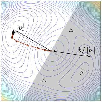
Figure 1: Contour plot of a two-dimensional instance of (1), featuring a local maximum ($\square$), saddle points ($\triangle$), and local minima ($\lozenge$). The line of circles indicates the path of gradient descent initialized at the origin, and the grey area is the half-plane $(v_{1}^{T}b)(v^{T}x)=b^{\left({1}\right)}x^{\left({1}\right)}>0$. Note that the global minimum is the only critical point outside this half-plane (Proposition 2.2). The gradient descent iterates have increasing norm (Lemma 2.3), lie outside the half-plane (Lemma 2.4), and converge to $x_{\star}$ (Proposition 2.5).

The gradient descent method begins at some initialization $x_{0}\in\mathbb{R}^{d}$ and generates iterates via

$$x_{t+1}=x_{t}-\eta\nabla f(x_{t})=(I-\eta A-\rho\eta\left\|{x_{t}}\right\|I)x_{t}-\eta b,$$ (9)

where $\eta$ is a fixed step size. Recalling the definitions (7a) and (8) of $R$ and $R_{c}$ as well as $\left\|{A}\right\|_{2}=\beta$, throughout our analysis we make the following assumptions.

Assumption A.

The step size $\eta$ in (9) satisfies $0<\eta\leq\frac{1}{4(\beta+\rho R)}$.

Assumption B.

The initialization of (9) satisfies $x_{0}=-r\frac{b}{\left\|{b}\right\|}$, with $0\leq r\leq R_{c}$.

To select a step size $\eta$ satisfying Assumption A, only a rough upper bound on $\left\|{A}\right\|_{2}$ is necessary. One way to obtain such a bound (with high probability) is to apply a few power iterations on $A$. Alternatively, we may perform line search, as in Section 5.

We begin our treatment of the convergence of gradient descent by establishing that $\|x_{t}\|$ is monotonic and bounded (see Appendix A for a proof).

Lemma 2.3.

Let Assumptions A and B hold. Then the iterates (9) of gradient descent satisfy $x_{t}^{T}\nabla f(x_{t})\leq 0$, the norms $\left\|{x_{t}}\right\|$ are non-decreasing, and $\left\|{x_{t}}\right\|\leq R$.

This lemma is the key to our analysis throughout the paper. The next lemma shows that $x_{t}$ and $b$ have opposite signs at all coordinates in the eigenbasis of $A$.

Lemma 2.4.

Let Assumptions A and B hold. For all $t\geq 0$ and $i\in\{1,...,d\}$

$$x_{t}^{(i)}b^{(i)}\leq 0,~{}b^{(i)}x_{\star}^{(i)}\leq 0,~{}\text{and}~{}x_{t}^{(i)}x_{\star}^{(i)}\geq 0.$$

Consequently, $x_{t}^{T}b\leq 0$ and $x_{t}^{T}x_{\star}\geq 0$ for every $t$, and $x_{\star}^{T}b\leq 0$.

Proof.    We first show that $x_{t}^{(i)}b^{(i)}\leq 0$. Writing the gradient descent recursion in the eigenbasis of $A$, we have

$$x_{t}^{(i)}=\left(1-\eta\lambda^{(i)}(A)-\eta\rho\|x_{t-1}\|\right)x_{t-1}^{(i)}-\eta b^{(i)}.$$ (10)

Assumption A and Lemma 2.3 imply $1-\eta\lambda^{(i)}(A)-\eta\rho\|x_{t-1}\|\geq 1-\eta(\beta+\rho R)>0$ for all $t,i$. Therefore, $x_{t}^{(i)}b^{(i)}\leq 0$ if $x_{0}^{(i)}b^{(i)}\leq 0$; the initialization in Assumption B guarantees this. To show $b^{(i)}x_{\star}^{(i)}\leq 0$, we use the fact that $b=-A_{\star}x_{\star}$ to write

$$b^{(i)}x_{\star}^{(i)}=-\left(\lambda^{(i)}(A)+\rho\|x_{\star}\|\right)[x_{\star}^{(i)}]^{2}\leq 0$$

as $\lambda^{(i)}(A)+\rho\|x_{\star}\|\geq 0$ for every $i$ by the condition (4) defining $x_{\star}$.

Multiplying $x_{t}^{(i)}b^{(i)}\leq 0$ and $b^{(i)}x_{\star}^{(i)}\leq 0$ yields $x_{t}^{(i)}x_{\star}^{(i)}[b^{(i)}]^{2}\geq 0$. The coordinate-wise update (10) and Assumption B show that $b^{(i)}=0$ implies $x_{t}^{(i)}=0$ for every $t$, and therefore $x_{t}^{(i)}x_{\star}^{(i)}\geq 0$. ∎

Lemmas 2.3, 2.4, and Proposition 2.2 immediately lead to the following guarantee.

Proposition 2.5.

Let Assumptions A and B hold, and assume that $b^{\left({1}\right)}\neq 0$. Then $x_{t}\to x_{\star}$ and $f(x_{t})\downarrow f(x_{\star})$ as $t\to\infty$.

Proof.    By Lemma 2.3, the iterates satisfy $\|x_{t}\|\leq R$ for all $t$. Since $\left\|{\nabla^{2}f(x)}\right\|_{2}\leq\beta+2\rho\left\|{x}\right\|$, the function $f$ is $\beta+2\rho R$-smooth on the set $\{x\in\mathbb{R}^{d}:\left\|{x}\right\|\leq R\}$ containing all the iterates $x_{t}$. Therefore, by the definition of smoothness and the gradient step,

$$f(x_{t+1})\leq f(x_{t})-\eta\|\nabla f(x_{t})\|^{2}+\frac{\eta^{2}}{2}(\beta+2\rho R)\|\nabla f(x_{t})\|^{2}\leq f(x_{t})-\frac{\eta}{2}\|\nabla f(x_{t})\|^{2}\ ,$$

where final inequality used Assumption A that $\eta\leq\frac{1}{4(\beta+\rho R)}$. Consequently, $f(x_{t})$ is decreasing and for every $t>0$,

$$\frac{\eta}{2}\sum_{\tau=0}^{t-1}\|\nabla f(x_{\tau})\|^{2}\leq f(x_{0})-f(x_{t})\leq f(x_{0})-f(x_{\star}).$$ (11)

Let $x_{\star}^{\prime}$ be any limit point of the sequence $x_{t}$ (there must be at least one, as the sequence $x_{t}$ is bounded). Inequality (11) implies $\nabla f(x_{t})\to 0$ and therefore $\nabla f(x_{\star}^{\prime})=0$ by continuity. By Lemma 2.4, $x_{t}^{(1)}b^{(1)}\leq 0$ for every $t$, so ${x_{\star}^{\prime}}^{\left({1}\right)}b^{\left({1}\right)}\leq 0$. Proposition 2.2 thus implies that $x_{\star}^{\prime}$ is the unique global minimizer $x_{\star}$. We conclude that $x_{\star}$ is the only limit point of the sequence $x_{t}$. ∎

To handle the case $b^{(1)}=0$, let $k\geq 1$ be the first index for which $b^{(k)}\neq 0$ (if no such $k$ exists then $b=0$ and $x_{t}=0$ for all $t$). Consider a modified problem instance, with $b,\rho$ unchanged but $A$ replaced with $\tilde{A}=\beta\sum_{i=1}^{k-1}v_{i}v_{i}^{T}+\lambda^{\left({i}\right)}(A)v_{i}v_{i}^{T}$, i.e. we replace the $k-1$ smallest eigenvalues with $\beta\geq\lambda^{\left({d}\right)}(A)$. Note that gradient descent produces the same iterates on the modified and original problems. Additionally, note that Lemma 2.3 and Proposition 2.5 apply to the modified problem, as the inner product between $b$ and the eigenvector of $\tilde{A}$ corresponding to its smallest eigenvalue is non-zero. Applying these results, we have $\left\|{x_{t}}\right\|\uparrow\left\|{\hat{x}_{\star}}\right\|$, where $\hat{x}_{\star}$ is the unique solution of the modified problem. Finally, we have $\left\|{\hat{x}_{\star}}\right\|\leq\left\|{x_{\star}}\right\|$, since $\hat{x}_{\star}\neq x_{\star}$ only if $\rho\left\|{\hat{x}_{\star}}\right\|\leq\gamma$ [7, Sec. 6.1]. Thus, we obtain the following lemma, to which we will refer throughout the sequel.

Lemma 2.6.

Let Assumptions A and B hold. For all $t\geq 0$, the iterates (9) of gradient descent satisfy $x_{t}^{T}\nabla f(x_{t})\leq 0$, the norms $\left\|{x_{t}}\right\|$ are non-decreasing and satisfy $\left\|{x_{t}}\right\|\leq\left\|{x_{\star}}\right\|$, and $f$ is ($\beta+2\rho\left\|{x_{\star}}\right\|$)-smooth on a ball containing the iterates $x_{t}$.

Figure 1 provides a graphical representation of these results, showing gradient descent’s iterates on an instance of problem (1) exhibiting numerous stationary points.

3 Non-asymptotic convergence rates

Proposition 2.5 shows the convergence of gradient descent for the cubic-regularized (non-convex) quadratic problem (1). We now present stronger non-asymptotic guarantees, including a randomized scheme solving (1) in all cases. We follow with simulations illustrating our theoretical results.

3.1 Theoretical results

Our primary result, Theorem 3.1, gives a convergence rate for gradient descent in the case that $b^{\left({1}\right)}\neq 0$. (Recall our convention (3), that parenthesized superscripts denote components in the eigenbasis of $A$). Further recalling that $\gamma=-\lambda^{\left({1}\right)}(A)$, $\beta=\left\|{A}\right\|_{2}$, $\mathsf{gap}$ is the eigengap of $A$, we define the shorthand

$$\gamma_{+}\triangleq\max\{\gamma,0\}~{}~{}\mbox{and}~{}~{}\mathsf{gap}^{\prime}\triangleq\min\{\mathsf{gap},\rho\left\|{x_{\star}}\right\|\}.$$

With this notation in hand, we state our result as follows.

Theorem 3.1.

Let Assumptions A and B hold, $b^{\left({1}\right)}\neq 0$, and $\varepsilon>0$. Then $f(x_{t})\leq f(x_{\star})+\varepsilon$ for all

$$t\geq T_{\varepsilon}\triangleq\frac{\tau_{\mathrm{grow}}(b^{(1)})+\tau_{\mathrm{conv}}\left(\varepsilon\right)}{\eta}\begin{cases}\frac{1}{\rho\left\|{x_{\star}}\right\|-\gamma}&\frac{1}{\rho\left\|{x_{\star}}\right\|-\gamma}\leq\frac{10\left\|{x_{\star}}\right\|^{2}}{\varepsilon}\vspace{5pt}\\ \sqrt{\frac{10\left\|{x_{\star}}\right\|^{2}}{\varepsilon}\cdot\frac{1}{\mathsf{gap}^{\prime}}}&\frac{1}{\mathsf{gap}^{\prime}}\leq\frac{10\left\|{x_{\star}}\right\|^{2}}{\varepsilon}\leq\frac{1}{\rho\left\|{x_{\star}}\right\|-\gamma}\vspace{5pt}\\ \frac{10\left\|{x_{\star}}\right\|^{2}}{\varepsilon}&\textnormal{otherwise}\end{cases}$$ (12)

where

$$\tau_{\mathrm{grow}}(b^{\left({1}\right)})=6\log\left(1+\frac{\gamma_{+}^{2}}{4\rho|b^{\left({1}\right)}|}\right)~{}\mbox{and}~{}\tau_{\mathrm{conv}}(\varepsilon)=6\log\left(\frac{(\beta+2\rho\left\|{x_{\star}}\right\|)\left\|{x_{\star}}\right\|^{2}}{\varepsilon}\right).$$

See Section 4.1 for a proof.

Theorem 3.1 shows that the rate of convergence changes from roughly $O(1/\varepsilon)$ to $O(\log(1/\varepsilon))$ as $\varepsilon$ decreases, with an intermediate gap-dependent rate of $O(1/\sqrt{\varepsilon})$. The terms $\tau_{\mathrm{grow}}$ and $\tau_{\mathrm{conv}}$ correspond to a period ($\tau_{\mathrm{grow}}$) in which $\left\|{x_{t}}\right\|$ grows exponentially in $t$ until reaching the basin of attraction to the global minimum and a period ($\tau_{\mathrm{conv}}$) of linear convergence to $x_{\star}$. Exponential growth occurs only in non-convex problem instances, as $\tau_{\mathrm{grow}}=0$ when the problem is convex.

The dependence of our result on $|b^{\left({1}\right)}|$ (the magnitude of $b$ in along the direction of the smallest eigenvector of $A$) is unavoidable: if $b^{\left({1}\right)}=0$, then gradient descent always remains in a subspace orthogonal to the smallest eigenvector of $A$, while $x_{\star}^{\left({1}\right)}$ might be non-zero; this is the “hard case” of non-convex quadratic problems [9, 7]. We use a small random perturbation to guarantee $|b^{\left({1}\right)}|\neq 0$ except with negligible probability, which yields the following high probability guarantee, whose proof we provide in Section 4.2.

Theorem 3.2.

Let Assumptions A and B hold, $\varepsilon,\delta>0$, and let $q$ be uniformly distributed on the unit sphere in $\mathbb{R}^{d}$. Let $\tilde{x}_{t}$ be generated by the gradient descent iteration (9) with $\tilde{b}=b+\sigma q$ replacing $b$, where

$$\sigma=\frac{\rho\varepsilon^{2}}{200(\beta+2\rho\left\|{x_{\star}}\right\|)^{2}\left\|{x_{\star}}\right\|^{2}}\cdot\overline{\sigma}~{}\mbox{with}~{}\overline{\sigma}\leq 1.$$

Then with probability at least $1-\delta$, we have $f(\tilde{x}_{t})\leq f(x_{\star})+(1+\overline{\sigma})\varepsilon$ for all

$$t\geq T_{\varepsilon}\triangleq\frac{\tilde{\tau}_{\mathrm{grow}}(d,\delta,\overline{\sigma})+\tilde{\tau}_{\mathrm{conv}}\left(\varepsilon\right)}{(1+\sqrt{\overline{\sigma}})^{-2}\eta}\begin{cases}\frac{1}{\rho\left\|{x_{\star}}\right\|-\gamma}&\frac{1}{\rho\left\|{x_{\star}}\right\|-\gamma}\leq\frac{10\left\|{x_{\star}}\right\|^{2}}{\varepsilon}\vspace{5pt}\\ \sqrt{\frac{10\left\|{x_{\star}}\right\|^{2}}{\varepsilon}\cdot\frac{1}{\mathsf{gap}^{\prime}}}&\frac{1}{\mathsf{gap}^{\prime}}\leq\frac{10\left\|{x_{\star}}\right\|^{2}}{\varepsilon}\leq\frac{1-2\sqrt{\overline{\sigma}}/3}{\rho\left\|{x_{\star}}\right\|-\gamma}\vspace{5pt}\\ \frac{10\left\|{x_{\star}}\right\|^{2}}{\varepsilon}&\textnormal{otherwise}\end{cases}$$ (13)

where

$$\tilde{\tau}_{\mathrm{grow}}(d,\delta,\overline{\sigma})\triangleq 6\log\left(1+\mathbb{I}_{\{\gamma>0\}}\frac{50\sqrt{d}}{\overline{\sigma}\delta}\right)~{}\mbox{and}~{}\tilde{\tau}_{\mathrm{conv}}(\varepsilon)\triangleq 20\log\left(\frac{(\beta+2\rho\left\|{x_{\star}}\right\|)\left\|{x_{\star}}\right\|^{2}}{\varepsilon}\right)\!\!.$$

To facilitate later discussion, we define $L_{\star}\triangleq\beta+2\rho\left\|{x_{\star}}\right\|$; then $f$ is $L_{\star}$-smooth on the Euclidean ball of radius $\left\|{x_{\star}}\right\|$. The bound (7b) implies $\rho R\leq\beta+\rho\left\|{x_{\star}}\right\|$, and therefore the step size choice $\eta=\frac{1}{4(\beta+\rho R)}$ satisfies $\frac{1}{\eta}\leq 8\beta+4\rho\left\|{x_{\star}}\right\|\leq 8L_{\star}$. Combining this upper bound with Theorem 3.2, we have the following corollary.

Corollary 3.3.

Let the conditions of Theorem 3.2 hold, $\eta=\frac{1}{4(\beta+\rho R)}$ and $\overline{\sigma}=1$. Then with probability at least $1-\delta$, we have $f(\tilde{x}_{t})\leq f(x_{\star})+\varepsilon$ for all

$$t\geq\tilde{T}_{\varepsilon}=O(1)\cdot\min\left\{\frac{L_{\star}}{\rho\left\|{x_{\star}}\right\|-\gamma},\frac{L_{\star}\left\|{x_{\star}}\right\|^{2}}{\varepsilon}\right\}\log\left[\left(1+\mathbb{I}_{\{\gamma>0\}}\frac{d}{\delta}\right)\frac{L_{\star}\left\|{x_{\star}}\right\|^{2}}{\varepsilon}\right].$$

We conclude the presentation of our main results with a few brief remarks.

1. Corollary 3.3 highlights parallels between our guarantees and those for gradient descent on smooth convex functions [23]. In our case, $L_{\star}/(\rho\left\|{x_{\star}}\right\|-\gamma)\geq 1$ is a condition number, while $L_{\star}$ and $\left\|{x_{\star}}\right\|$ bound the smoothness of $f$ and iterate radius $\sup_{t}\left\|{x_{t}}\right\|$, respectively. We defer further comparison to Section 7.

2. We readily obtain relative accuracy guarantees by using the bound (5a); setting $\varepsilon=\rho\left\|{x_{\star}}\right\|^{3}\varepsilon^{\prime}/12$, we have $f(\tilde{x}_{t})-f(x_{\star})\leq-\varepsilon^{\prime}f(x_{\star})=\varepsilon^{\prime}(f(0)-f(x_{\star}))$, or $f(\tilde{x}_{t})\leq(1-\varepsilon^{\prime})f(x_{\star})$, for any $t\geq\tilde{T}_{\varepsilon}$, where $\tilde{T}_{\varepsilon}$ is defined in (13).

3. Evaluating $\tilde{T}_{\varepsilon}$ for given $A$, $b$ and $\rho$ is not straightforward, as $\left\|{x_{\star}}\right\|$ is generally unknown. Using $\left\|{x_{\star}}\right\|\leq R$ gives an easily computable upper bound on $\tilde{T}_{\varepsilon}$, and in Section 6, we demonstrate how to apply our results when $\left\|{x_{\star}}\right\|$ is unknown.

3.2 Illustration of results

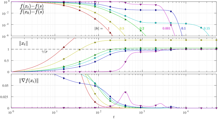
Figure 2: Trajectories of gradient descent with $\lambda^{(1)}(A)=-\gamma=-0.2$ and $\lambda^{(2)}(A),...,\lambda^{(d)}(A)$ equally spaced between $-0.18$ and $\beta=1$, and different vectors $b$ proportional to $[0.01,1,1,1,\ldots]$ in the eigenbasis of $A$. The rest of the parameters are $d=10^{3}$, $\eta=0.1$, $\rho=0.2$ and $x_{0}=0$.

We present two experiments that investigate the behavior of gradient descent on problem (1). For the first experiment, we examine the behavior of gradient descent on single problem instances, looking at convergence behavior as we vary the vector $b$ (to effect conditioning of the problem) by scaling its norm $\left\|{b}\right\|$. The selected norm values $\left\|{b}\right\|\in\{1,0.5,0.2,0.15,0.1,0.001\}$ correspond to condition numbers $(\beta+\rho\left\|{x_{\star}}\right\|)/(-\gamma+\rho\left\|{x_{\star}}\right\|)\in\{7.6,16,120,5.5\cdot 10^{3},2.9\cdot 10^{4},3.8\cdot 10^{6}\}$; the problem conditioning becomes worse as $\left\|{b}\right\|$ decreases. Figure 2 summarizes our results and describes the settings of the other parameters in the experiment.

The plots show two behaviors of gradient descent. The problem is well-conditioned when $\|b\|\geq 0.2$, and in these cases gradient descent behaves as though the problem was strongly convex, with $x_{t}$ converging linearly to $x_{\star}$. For $\|b\|\leq 0.15$ the problem becomes ill-conditioned and gradient descent stalls around saddle points. Indeed, the third plot of Figure 2 shows that for the ill-conditioned problems, we have $\left\|{\nabla f(x_{t})}\right\|$ increasing over some iterations, which does not occur in convex quadratic problems. The length of the stall does not depend only on the condition number; for $\left\|{b}\right\|=10^{-3}$ the stall is shorter than for $\left\|{b}\right\|\in\{0.1,0.15\}$. Instead, it appears to depend on the norm of the saddle point which causes it, which we observe from the value of $\left\|{x_{t}}\right\|$ at the time of the stall; we see that the closer the norm is to $\gamma/\rho$, the longer the stall takes. This is explained by observing that $\nabla^{2}f(x)\succeq(\rho\left\|{x}\right\|-\gamma)I$, which means that every saddle point with norm close to $\gamma/\rho$ must have only small negative curvature, and therefore harder to escape (see also Lemma 4.3 in the sequel). Fortunately, as we see in Fig. 2, saddle points with large norm have near-optimal objective value—this is the intuition behind our proof of the sub-linear convergence rates.

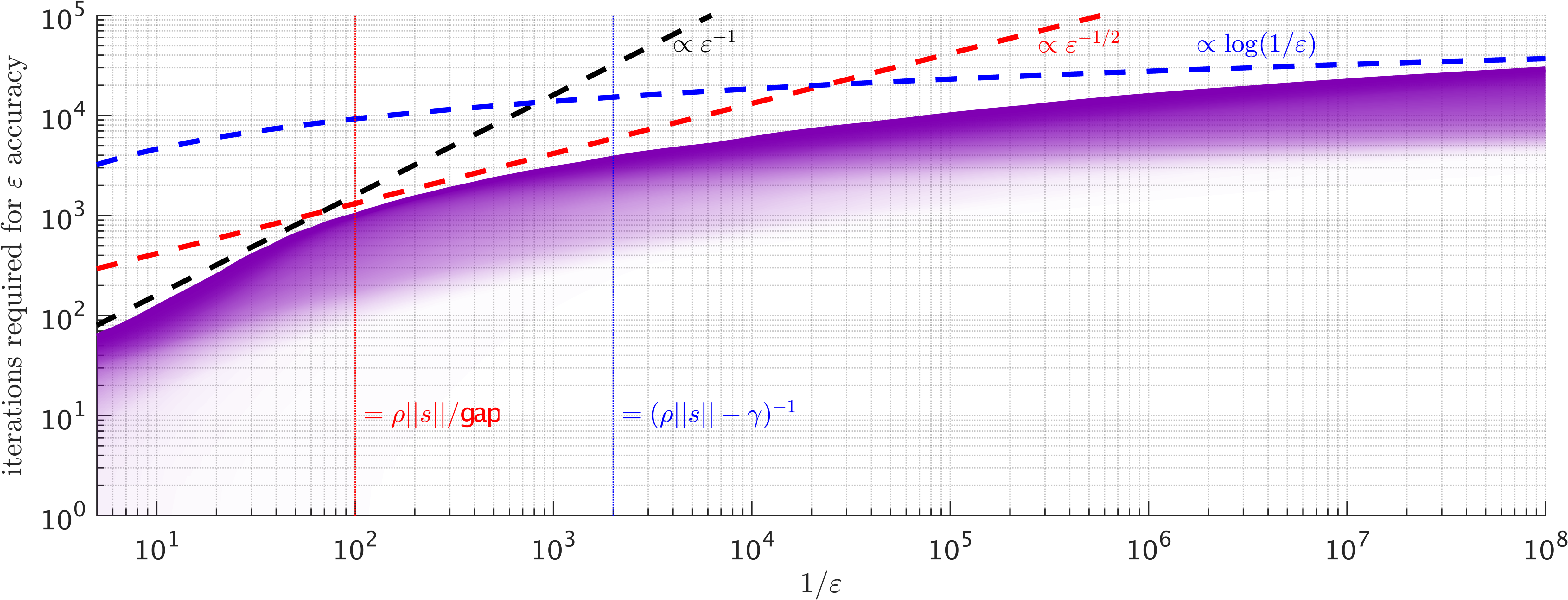
Figure 3: The purple curve is shaded according to the cdf of the number of iterations required to reach relative accuracy $\varepsilon$, computed over $2{,}500$ random problem instances each with $d=10^{4}$, $\beta=\rho=1$, $\gamma=0.5$, $\mathsf{gap}=5\cdot 10^{-3}$ and $\rho\left\|{x_{\star}}\right\|-\gamma=5\cdot 10^{-4}$. We use $x_{0}=-R_{c}b/\|b\|$ and $\eta=0.25$. The black, red and blue dashed curves indicate the three convergence regimes Theorem 3.1 identifies.

In our second experiment, we test our rate guarantees by considering the performance of gradient descent over an ensemble of random instances. We generate random instances with a fixed value of $\gamma$, $\beta$, $\rho$, $\left\|{x_{\star}}\right\|$ and $\mathsf{gap}$ as follows. We set $A=\mathop{\rm diag}([-\gamma;-\gamma+\mathsf{gap};u])$ with $u$ uniformly random in $[-\gamma+\mathsf{gap},\beta]^{d-2}$. We draw $\check{x_{\star}}=(A+\rho\left\|{x_{\star}}\right\|)^{-\zeta}\nu$, where $\nu\sim\mathcal{N}(0;I)$ and $\log_{2}\zeta$ is uniform on $[-1,1]$. We then set $x_{\star}=(\left\|{x_{\star}}\right\|/\left\|{\check{x_{\star}}}\right\|)\check{x_{\star}}$ and $b=-(A+\rho\left\|{x_{\star}}\right\|)x_{\star}$, so that $x_{\star}$ is the global minimizer of problem instance $(A,b,\rho)$. The choice of $\zeta$ ensures we observe large variety in the values of $\left\|{x_{t}}\right\|$ at which gradient descent stalls, allowing us to find difficult instances for each value of $\varepsilon$. In Figure 3 we depict the cumulative distribution of the number of iterations required to find an $\varepsilon$-relatively-accurate solution versus $1/\varepsilon$. The slopes in the plot agree with our upper bounds, suggesting the sharpness of our theoretical results.

4 Proofs of main results

In this section, we provide proofs of our main results, Theorems 3.1 and 3.2. A number of the steps involve technical lemmas whose proofs we defer to Appendix B. In all lemma statements, we tacitly let Assumptions A and B hold, as in the main theorem statements. Without loss of generality, we assume $\varepsilon\leq\frac{1}{2}\beta\left\|{x_{\star}}\right\|^{2}+\rho\left\|{x_{\star}}\right\|^{3}$, as $f$ is $\beta+2\rho\left\|{x_{\star}}\right\|$ smooth on the set $\{x:\left\|{x}\right\|\leq\left\|{x_{\star}}\right\|\}$ and therefore $f(x_{0})\leq f(x_{\star})+\varepsilon$ for any $\varepsilon\geq\frac{1}{2}\beta\left\|{x_{\star}}\right\|^{2}+\rho\left\|{x_{\star}}\right\|^{3}$.

4.1 Proof of Theorem 3.1

We divide the proof of Theorem 3.1 into two main steps: in Section 4.1.1 we prove the first case in the bound (12) (linear convergence), and in Section 4.1.2 we prove the last two cases in (12) (sublinear convergence).

4.1.1 Linear convergence and exponential growth

We first prove that $f(x_{t})\leq f(x_{\star})+\varepsilon$ for $t\geq\frac{1}{\eta(\rho\left\|{x_{\star}}\right\|-\gamma)}(\tau_{\mathrm{grow}}(b^{\left({1}\right)})+\tau_{\mathrm{conv}}(\varepsilon))$. We begin with two lemmas that provide regimes in which $x_{t}$ converges to the solution $x_{\star}$ linearly.

Lemma 4.1.

For each $t>0$, we have

$$\left\|{x_{t}-x_{\star}}\right\|^{2}\leq\left(1-\eta\left[\rho\left\|{x_{t}}\right\|-\left(\gamma-\frac{\rho\left\|{x_{\star}}\right\|-\gamma}{2}\right)\right]\right)\left\|{x_{t-1}-x_{\star}}\right\|^{2}$$

See Appendix B.1 for a proof of this lemma.

For non-convex problem instances (those with $\gamma>0$), the above recursion is a contraction (implying linear convergence of $x_{t}$ to $x_{\star}$) only when $\rho\left\|{x_{t}}\right\|$ is larger than $\gamma-\frac{1}{2}(\rho\left\|{x_{\star}}\right\|-\gamma)$. Using the fact that $\|x_{t}\|$ is non-decreasing (Lemma 2.6), Lemma 4.1 immediately implies the following result.

Lemma 4.2.

If $\rho\|x_{t}\|\geq\gamma-\frac{1}{2}\left(\rho\left\|{x_{\star}}\right\|-\gamma\right)+\mu$ for some $t\geq 0$, then for all $\tau\geq 0$,

$$\|x_{t+\tau}-x_{\star}\|^{2}\leq\left(1-\eta\mu\right)^{\tau}\|x_{t}-x_{\star}\|^{2}\leq 2\left\|{x_{\star}}\right\|^{2}e^{-\eta\mu\tau}.$$

Proof.    Lemma 4.1 implies that $\left\|{x_{t+\tau}-x_{\star}}\right\|^{2}\leq(1-\eta\mu)\left\|{x_{t+\tau-1}-x_{\star}}\right\|^{2}$ for all $\tau>1$. Using that $\left\|{x_{t}-x_{\star}}\right\|^{2}\leq\left\|{x_{t}}\right\|^{2}+\left\|{x_{\star}}\right\|^{2}\leq 2\left\|{x_{\star}}\right\|^{2}$ by Lemma 2.4, Lemma 2.6, and $1+\alpha\leq e^{\alpha}$ for all $\alpha$ gives the result. ∎

It remains to understand whether the gradient descent iterations satisfy the condition $\rho\|x_{t}\|\geq\gamma-\frac{1}{2}\left(\rho\left\|{x_{\star}}\right\|-\gamma\right)+\mu$. Fortunately, as long as $\rho\|x_{t}\|$ is below $\gamma-\nu$, $|x_{t}^{\left(1\right)}|$ grows faster than $(1+\eta\nu)^{t}$:

Lemma 4.3.

Let $\nu>0$. Then $\rho\|x_{t}\|\geq\gamma-\nu$ for all $t\geq\frac{2}{\eta\nu}\log(1+\frac{\gamma_{+}^{2}}{4\rho|b^{\left(1\right)}|})$.

See Appendix B.2 for a proof of this lemma.

We now combine the lemmas to give the linear convergence regime of Theorem 3.1. Applying Lemma 4.3 with $\nu=\frac{1}{3}(\rho\left\|{x_{\star}}\right\|-\gamma)$ yields $\rho\left\|{x_{t}}\right\|\geq\gamma-\frac{1}{3}\left(\rho\left\|{x_{\star}}\right\|-\gamma\right)$ for

$$t\geq T_{1}\triangleq\frac{6}{\eta\left(\rho\left\|{x_{\star}}\right\|-\gamma\right)}\log\left(1+\frac{\gamma_{+}^{2}}{4\rho|b^{\left(1\right)}|}\right)=\frac{1}{\eta(\rho\left\|{x_{\star}}\right\|-\gamma)}\tau_{\mathrm{grow}}(b^{\left({1}\right)}).$$

Therefore, by Lemma 4.2 with $\mu=\frac{1}{2}(\rho\left\|{x_{\star}}\right\|-\gamma)-\nu=\frac{1}{6}(\rho\left\|{x_{\star}}\right\|-\gamma)$, for any $t$ we have

$$\left\|{x_{T_{1}+t}-x_{\star}}\right\|^{2}\leq 2\left\|{x_{\star}}\right\|^{2}\exp\Big{(}-\frac{1}{6}\eta\left(\rho\left\|{x_{\star}}\right\|-\gamma\right)t\Big{)}.$$ (14)

As a consequence, for all $t\geq 0$ we may use the $(\beta+2\rho\left\|{x_{\star}}\right\|)$-smoothness of $f$ and the fact that $\left\|{x_{t}}\right\|\leq\left\|{x_{\star}}\right\|$ (by Lemma 2.6) to obtain

$$f\left(x_{t}\right)-f\left(x_{\star}\right)\leq\frac{\beta+2\rho\left\|{x_{\star}}\right\|}{2}\left\|{x_{t}-x_{\star}}\right\|^{2}\leq(\beta+2\rho\left\|{x_{\star}}\right\|)\left\|{x_{\star}}\right\|^{2}e^{-\frac{1}{6}\eta(\rho\left\|{x_{\star}}\right\|-\gamma)(t-T_{1})}$$

where we have used that $\nabla f(x_{\star})=0$ and the bound (14). Therefore, if we set

$$T_{2}\triangleq\frac{6}{\eta\left(\rho\left\|{x_{\star}}\right\|-\gamma\right)}\log\frac{(\beta+2\rho\left\|{x_{\star}}\right\|)\left\|{x_{\star}}\right\|^{2}}{\varepsilon}=\frac{1}{\eta(\rho\left\|{x_{\star}}\right\|-\gamma)}\tau_{\mathrm{conv}}(\varepsilon),$$

then $t\geq T_{1}+T_{2}=\frac{1}{\eta(\rho\left\|{x_{\star}}\right\|-\gamma)}(\tau_{\mathrm{grow}}(b^{\left({1}\right)})+\tau_{\mathrm{conv}}(\varepsilon))$ implies $f(x_{t})-f(x_{\star})\leq\varepsilon$.

4.1.2 Sublinear convergence and convergence in subspaces

We now turn to the sublinear convergence regime in Theorem 3.1, which applies when the quantity $\rho\left\|{x_{\star}}\right\|-\gamma$ is sufficiently small.

$$\rho\left\|{x_{\star}}\right\|-\gamma\leq\frac{\varepsilon}{10\left\|{x_{\star}}\right\|^{2}}~{}.$$ (15)

Note that if (15) fails to hold, then (12) is dominated by the $(\rho\left\|{x_{\star}}\right\|-\gamma)^{-1}$ term. Therefore, to complete the proof of Theorem 3.1 it suffices to show that if (15) holds, then $f(x_{t})\leq f(x_{\star})+\varepsilon$ whenever

$$t\geq T^{\rm sub}_{\varepsilon}\triangleq\frac{\tau_{\mathrm{grow}}(b^{\left({1}\right)})+\tau_{\mathrm{conv}}(\varepsilon)}{\eta}\min\left\{\frac{10\left\|{x_{\star}}\right\|^{2}}{\varepsilon},\sqrt{\frac{10\left\|{x_{\star}}\right\|^{2}}{(\min\{\mathsf{gap},\rho\left\|{x_{\star}}\right\|\})\varepsilon}}\right\}.$$ (16)

Roughly, our proof of the result (16) proceeds as follows: when $\rho\left\|{x_{\star}}\right\|-\gamma$ is small, the function $f$ is very smooth along eigenvectors with eigenvalues close to $-\gamma=\lambda^{\left({1}\right)}(A)$. It is therefore sufficient to show convergence in the complementary subspace, which occurs at a linear rate. Appropriately choosing the gap between the eigenvalues in the complementary subspace and $\lambda^{\left({1}\right)}(A)$ to trade between convergence rate and function smoothness yields the rates (16).

The following analogs of Lemmas 4.1 and 4.2 establish subspace convergence.

Lemma 4.4.

Let $\Pi$ be any projection matrix satisfying $\Pi A=A\Pi$ for which $\Pi A_{\star}\succeq\nu\Pi$ for some $\nu>0$. For all $t>0$,

$$\|{\Pi A_{\star}^{1/2}(x_{t}-x_{\star})}\|^{2}\leq\left(1-\eta\nu\right)\|{\Pi A_{\star}^{1/2}(x_{t-1}-x_{\star})}\|^{2}$$

$$\qquad+\sqrt{8}\eta\rho\left(\left\|{x_{\star}}\right\|-\left\|{x_{t-1}}\right\|\right)\left[\rho\left(\left\|{x_{\star}}\right\|-\left\|{x_{t-1}}\right\|\right)\left\|{x_{t-1}}\right\|^{2}+\left\|{(I-\Pi)A_{\star}}\right\|_{2}\left\|{x_{\star}}\right\|^{2}\right].$$

See Appendix B.3 for a proof. Letting $\Pi_{\nu}=\sum_{i:\lambda^{\left({i}\right)}\geq\nu+\lambda^{\left({1}\right)}}v_{i}v_{i}^{T}$ be the projection matrix onto the span of eigenvectors of $A$ with eigenvalues at least $\lambda^{\left({1}\right)}(A)+\nu$, we obtain the following consequence of Lemma 4.4, whose proof we provide in Appendix B.4.

Lemma 4.5.

Let $t\geq 0$, $\nu\geq 0$, and define $\bar{\nu}=\max\{\nu,\mathsf{gap}\}$. If $\rho\left\|{x_{\star}}\right\|\leq\gamma+\sqrt{\nu\bar{\nu}}$ and $\rho\left\|{x_{t}}\right\|\geq\gamma-\frac{1}{3}\sqrt{\nu\bar{\nu}}$, then for any $\tau\geq 0$,

$$\left\|{\Pi_{\nu}A_{\star}^{1/2}\left(x_{t+\tau}-x_{\star}\right)}\right\|^{2} \leq\left(1-\eta\bar{\nu}\right)^{\tau}\left\|{\Pi_{\nu}A_{\star}^{1/2}\left(x_{t}-x_{\star}\right)}\right\|^{2}+13\left\|{x_{\star}}\right\|^{2}\nu$$

$$\leq 2\left(\beta+\rho\left\|{x_{\star}}\right\|\right)\left\|{x_{\star}}\right\|^{2}e^{-\eta\bar{\nu}\tau}+13\left\|{x_{\star}}\right\|^{2}\nu.$$

We use these lemmas to prove the desired bound (16) by appropriate separation of the eigenspaces over which we guarantee convergence. To that end, we define

$$\nu\triangleq\frac{\varepsilon}{10\left\|{x_{\star}}\right\|^{2}}~{}~{},~{}~{}\bar{\nu}\triangleq\max\{\nu,\mathsf{gap}\}~{}~{}\mbox{and}~{}~{}\bar{\nu}^{\prime}\triangleq\max\{{\nu},(\min\{\mathsf{gap},\rho\left\|{x_{\star}}\right\|\})\leq\bar{\nu}\},$$ (17)

and note that the definition of $\mathsf{gap}$ immediately implies $\Pi_{\nu}=\Pi_{\bar{\nu}}$. The growth guranteed by Lemma 4.3 shows that $\rho\left\|{x_{t}}\right\|\geq\gamma-\frac{1}{3}\sqrt{\nu\bar{\nu}^{\prime}}$ for every

$$t\geq T_{1}^{\rm sub}\triangleq\frac{6}{\eta\sqrt{\nu\bar{\nu}^{\prime}}}\log\left(1+\frac{\gamma_{+}^{2}}{4\rho|b^{\left(1\right)}|}\right)=\frac{1}{\eta\sqrt{\nu\bar{\nu}^{\prime}}}\tau_{\mathrm{grow}}(b^{\left({1}\right)}).$$

Additionally, for $t\geq T_{1}^{\rm sub}$ we have $\rho\left\|{x_{t}}\right\|\geq\gamma-\frac{1}{3}\sqrt{\nu\bar{\nu}^{\prime}}\geq\gamma-\frac{1}{3}\sqrt{\nu\bar{\nu}}$ because $\bar{\nu}\geq\bar{\nu}^{\prime}$. Thus, using that $\nu,\bar{\nu}^{\prime}\leq\bar{\nu}$ and that $(\beta+2\rho\left\|{x_{\star}}\right\|\left\|{x_{\star}}\right\|^{2}/\varepsilon\geq 2$ as in the beginning of Sec. 4, we may define

$$T_{2}^{\rm sub}\triangleq\frac{1}{\eta\bar{\nu}}\log\frac{2(\beta+\rho\left\|{x_{\star}}\right\|)}{\nu}\leq\frac{1}{\eta\sqrt{\nu\bar{\nu}^{\prime}}}\log\left(\left[\frac{(\beta+2\rho\left\|{x_{\star}}\right\|)\left\|{x_{\star}}\right\|^{2}}{\varepsilon}\right]^{6}\right)=\frac{\tau_{\mathrm{conv}}(\varepsilon)}{\eta\sqrt{\nu\bar{\nu}^{\prime}}}.$$

Thus $2(\beta+\rho\left\|{x_{\star}}\right\|)\left\|{x_{\star}}\right\|^{2}e^{-\eta\bar{\nu}t}\leq\left\|{x_{\star}}\right\|^{2}\nu$ for every $t\geq T_{2}^{\rm sub}$, and by Lemma 4.5 we have

$$\left\|{\Pi_{\nu}A_{\star}^{1/2}(x_{t}-x_{\star})}\right\|^{2}\leq\left\|{x_{\star}}\right\|^{2}\nu+13\left\|{x_{\star}}\right\|^{2}\nu=14\left\|{x_{\star}}\right\|^{2}\nu,$$ (18)

for every $t\geq T^{\rm sub}=T_{1}^{\rm sub}+T_{2}^{\rm sub}$.

We now translate the guarantee (18) on the distance from $x_{t}$ to $x_{\star}$ in the subspace of “large” eigenvectors of $A$ to a guarantee on the solution quality $f(x_{t})$. Using the expression (6) for $f(x)$, the orthogonality of $I-\Pi_{\nu}$ and $\Pi_{\nu}$ and $\left\|{x_{t}}\right\|\leq\left\|{x_{\star}}\right\|$, we have

$$f(x_{t})\leq f(x_{\star})+\frac{1}{2}\left\|{(I-\Pi_{\nu})A_{\star}^{\frac{1}{2}}(x_{t}-x_{\star})}\right\|^{2}+\frac{1}{2}\left\|{\Pi_{\nu}A_{\star}^{\frac{1}{2}}(x_{t}-x_{\star})}\right\|^{2}+\frac{\rho\left\|{x_{\star}}\right\|}{2}(\left\|{x_{\star}}\right\|-\left\|{x_{t}}\right\|)^{2}.$$

Now we note that

$$\left\|{(I-\Pi_{\nu})A_{\star}}\right\|_{2}=\max_{i:\lambda^{\left({i}\right)}<\lambda^{\left({1}\right)}+\nu}|\lambda^{\left({i}\right)}+\rho\left\|{x_{\star}}\right\||\leq-\gamma+\nu+\rho\left\|{x_{\star}}\right\|\leq 2\nu,$$ (19)

where we have used our assumption (15) that $\rho\left\|{x_{\star}}\right\|-\gamma\leq\frac{\varepsilon}{10\left\|{x_{\star}}\right\|^{2}}=\nu$. Using this gives

$$f(x_{t})\leq f(x_{\star})+\nu\left\|{x_{t}-x_{\star}}\right\|^{2}+7\left\|{x_{\star}}\right\|^{2}\nu+\frac{\rho\left\|{x_{\star}}\right\|}{2}(\left\|{x_{\star}}\right\|-\left\|{x_{t}}\right\|)^{2},$$ (20)

where we use inequality (18). Because $\rho\left\|{x_{t}}\right\|\geq\gamma-\frac{1}{3}\sqrt{\nu\bar{\nu}^{\prime}}$ for $t\geq T_{1}^{\rm sub}$, we obtain

$$0\leq\rho(\left\|{x_{\star}}\right\|-\left\|{x_{t}}\right\|)\leq\rho\left\|{x_{\star}}\right\|-\gamma-(\rho\left\|{x_{t}}\right\|-\gamma)\leq\frac{4}{3}\sqrt{\nu\bar{\nu}^{\prime}}.$$

The above inequality provides an upper bound on $(\left\|{x_{\star}}\right\|-\left\|{x_{t}}\right\|)^{2}$. Alternatively, we may bound $(\left\|{x_{\star}}\right\|-\left\|{x_{t}}\right\|)^{2}\leq\left\|{x_{\star}}\right\|^{2}$ using $\left\|{x_{t}}\right\|\leq\left\|{x_{\star}}\right\|$ (Lemma 2.6). Therefore

$$\frac{\rho\left\|{x_{\star}}\right\|}{2}(\left\|{x_{\star}}\right\|-\left\|{x_{t}}\right\|)^{2}\leq\left\|{x_{\star}}\right\|^{2}\min\left\{\frac{\rho\left\|{x_{\star}}\right\|}{2},\frac{16\bar{\nu}^{\prime}\nu}{18\rho\left\|{x_{\star}}\right\|}\right\}\leq\left\|{x_{\star}}\right\|^{2}\nu,$$ (21)

where the final inequality follows as $\bar{\nu}^{\prime}\leq\max\{\nu,\rho\left\|{x_{\star}}\right\|\}$. Substituting the bound (21) into (20) with $\left\|{x_{\star}-x_{t}}\right\|^{2}\leq 2\left\|{x_{\star}}\right\|^{2}$ (by Lemma 2.4), we find

$$f(x_{t})\leq f(x_{\star})+9\left\|{x_{\star}}\right\|^{2}\nu\leq f(x_{t})+\varepsilon,$$

where we substitute $\nu=\frac{\varepsilon}{10\left\|{x_{\star}}\right\|^{2}}$. Summarizing, if $\rho\left\|{x_{\star}}\right\|-\gamma\leq\nu=\frac{\varepsilon}{10\left\|{x_{\star}}\right\|^{2}}$, the point $x_{t}$ is $\varepsilon$-suboptimal for problem (1) whenever $t\geq\frac{\tau_{\mathrm{grow}}(b^{\left({1}\right)})+\tau_{\mathrm{conv}}(\varepsilon)}{\eta\sqrt{\nu\bar{\nu}^{\prime}}}\geq T_{1}^{\rm sub}+T_{2}^{\rm sub}$, where

$$\sqrt{\nu\bar{\nu}^{\prime}}=\max\left\{\frac{\varepsilon}{10\left\|{x_{\star}}\right\|^{2}},\sqrt{\frac{\varepsilon}{10\left\|{x_{\star}}\right\|^{2}}\min\{\mathsf{gap},\rho\left\|{x_{\star}}\right\|\}}\right\}.$$

4.2 Proof of Theorem 3.2

Theorem 3.2 follows from three basic observations about the effect of adding a small uniform perturbation to $b$, which we summarize in the following lemma (see Section B.5 for a proof).

Lemma 4.6.

Set $\tilde{b}=b+\sigma q$, where $q$ is uniform on the unit sphere in $\mathbb{R}^{d}$ and $\sigma>0$. Let $\tilde{f}\left(x\right)=\frac{1}{2}x^{T}Ax+\tilde{b}^{T}x+\frac{1}{3}\rho\left\|{x}\right\|^{3}$ and let $\tilde{x}_{\star}$ be a global minimizer of $\tilde{f}$. Then, for any $\delta>0$

1. For $d>2$, $\mathbb{P}(|\tilde{b}^{\left({1}\right)}|\leq\sqrt{\pi}\sigma\delta/\sqrt{2d})\leq\delta$

2. $|f(x)-\tilde{f}(x)|\leq\sigma\left\|{x}\right\|$ for all $x\in\mathbb{R}^{d}$

3. $\big{|}\left\|{x_{\star}}\right\|-\left\|{\tilde{x}_{\star}}\right\|\big{|}\leq\sqrt{2\sigma/\rho}$.

With Lemma 4.6 in hand, our proof proceeds in three parts: in the first two, we provide bounds on the iteration complexity of each of the modes of convergence that Theorem 3.1 exhibits in the perturbed problem with vector $\tilde{b}$. The final part shows that the quality of the (approximate) solutions $\tilde{x}_{t}$ and $\tilde{x}_{\star}$ is not much worse than $x_{\star}$.

Let $\tilde{f},\tilde{b}$ and $\tilde{x}_{\star}$ be as defined in Lemma 4.6. By Theorem 3.1, we know that $\tilde{f}(\tilde{x}_{t})\leq\tilde{f}(\tilde{x}_{\star})+\varepsilon$ for all

$$t\geq\frac{6}{\eta}\left(\log\left(1+\frac{\gamma_{+}^{2}/4}{\rho|\tilde{b}^{\left({1}\right)}|}\right)+\log\frac{(\beta+2\rho\left\|{\tilde{x}_{\star}}\right\|)\left\|{\tilde{x}_{\star}}\right\|^{2}}{\varepsilon}\right)\min\left\{\frac{1}{\rho\left\|{\tilde{x}_{\star}}\right\|-\gamma},\frac{10\left\|{\tilde{x}_{\star}}\right\|^{2}}{\varepsilon}\right\},$$ (22a)

and that if $$\rho\left\|{\tilde{x}_{\star}}\right\|-\gamma\leq\frac{\varepsilon}{10\left\|{\tilde{x}_{\star}}\right\|} \tilde{f}(\tilde{x}_{t})\leq\tilde{f}(\tilde{x}_{\star})+\varepsilon$$, then for all

$$t\geq\frac{6}{\eta}\left(\log\left(1+\frac{\gamma_{+}^{2}}{4\rho|\tilde{b}^{\left({1}\right)}|}\right)+\log\frac{(\beta+2\rho\left\|{\tilde{x}_{\star}}\right\|)\left\|{\tilde{x}_{\star}}\right\|^{2}}{\varepsilon}\right)\sqrt{\frac{10\left\|{\tilde{x}_{\star}}\right\|^{2}}{\varepsilon}\frac{1}{\min\{\mathsf{gap},\rho\left\|{\tilde{x}_{\star}}\right\|\}}}.$$ (22b)

We now turn to bounding expressions (22a) and (22b) appropriately: Section 4.2.1 deals with the occurrences of $\left\|{\tilde{x}_{\star}}\right\|$ outside the logarithm, and Section 4.2.2 bounds the terms $\tilde{b}^{\left({1}\right)}$ and $\left\|{\tilde{x}_{\star}}\right\|$ appearing inside the logarithm.

4.2.1 Part 1: upper bounding terms outside the log

Recalling that $\sigma=\frac{\rho\overline{\sigma}\varepsilon^{2}}{2(10\beta+20\rho\left\|{x_{\star}}\right\|)^{2}\left\|{x_{\star}}\right\|^{2}}$ and $\varepsilon\leq(\frac{1}{2}\beta+\rho\left\|{x_{\star}}\right\|)\left\|{x_{\star}}\right\|^{2}$, we have $\sigma\leq{\frac{1}{800}}\overline{\sigma}\rho\left\|{x_{\star}}\right\|^{2}$. Thus, part (iii) of Lemma 4.6 gives

$$|\left\|{x_{\star}}\right\|-\left\|{\tilde{x}_{\star}}\right\||\leq\sqrt{2\sigma/\rho}\leq\sqrt{\overline{\sigma}}\left\|{x_{\star}}\right\|/20,~{}~{}\mbox{so}~{}~{}\left\|{\tilde{x}_{\star}}\right\|\in(1\pm\sqrt{\overline{\sigma}}/20)\left\|{x_{\star}}\right\|.$$

Similarly, we have

$$\big{|}\left\|{x_{\star}}\right\|-\left\|{\tilde{x}_{\star}}\right\|\big{|}\leq\sqrt{\frac{\overline{\sigma}\varepsilon^{2}}{(10\beta+20\rho\left\|{x_{\star}}\right\|)^{2}\left\|{x_{\star}}\right\|^{2}}}\leq\frac{\sqrt{\overline{\sigma}}}{20}\frac{\varepsilon}{\rho\left\|{x_{\star}}\right\|^{2}}~{}.$$ (23)

Now, suppose that $\frac{\varepsilon}{10\left\|{x_{\star}}\right\|^{2}}\leq\rho\left\|{x_{\star}}\right\|-\gamma$. Substituting this into the bound (23) yields $|\left\|{x_{\star}}\right\|-\left\|{\tilde{x}_{\star}}\right\||\leq\frac{\sqrt{\overline{\sigma}}}{2\rho}(\rho\left\|{x_{\star}}\right\|-\gamma)$, and rearranging, we obtain

$$\rho\left\|{\tilde{x}_{\star}}\right\|-\gamma\geq\left(1-0.5\sqrt{\overline{\sigma}}\right)(\rho\left\|{x_{\star}}\right\|-\gamma)\geq\frac{\rho\left\|{x_{\star}}\right\|-\gamma}{1+\sqrt{\overline{\sigma}}}$$

because $\overline{\sigma}\leq 1$. We combine the preceding bounds to obtain

$$\min\left\{\frac{1}{\rho\left\|{\tilde{x}_{\star}}\right\|-\gamma},\frac{10\left\|{\tilde{x}_{\star}}\right\|^{2}}{\varepsilon}\right\}\leq(1+\sqrt{\overline{\sigma}})^{2}\min\left\{\frac{1}{\rho\left\|{{x_{\star}}}\right\|-\gamma},\frac{10\left\|{{x_{\star}}}\right\|^{2}}{\varepsilon}\right\}$$ (24a)

and

$$\sqrt{\frac{10\left\|{\tilde{x}_{\star}}\right\|^{2}}{\varepsilon}\cdot\frac{1}{\min\{\mathsf{gap},\rho\left\|{\tilde{x}_{\star}}\right\|\}}}\leq(1+\sqrt{\overline{\sigma}})\sqrt{\frac{10\left\|{{x_{\star}}}\right\|^{2}}{\varepsilon}\cdot\frac{1}{\min\{\mathsf{gap},\rho\left\|{x_{\star}}\right\|\}}}\ .$$ (24b)

The bound (23) also implies $\rho\left\|{\tilde{x}_{\star}}\right\|-\gamma\leq\rho\left\|{x_{\star}}\right\|-\gamma+\frac{\sqrt{\overline{\sigma}}\varepsilon}{20\left\|{x_{\star}}\right\|^{2}}$. When $\rho\left\|{x_{\star}}\right\|-\gamma\leq(1-2\sqrt{\overline{\sigma}}/3)\frac{\varepsilon}{10\left\|{x_{\star}}\right\|^{2}}$, we thus have

$$\rho\left\|{\tilde{x}_{\star}}\right\|-\gamma\leq\frac{\varepsilon}{10\left\|{x_{\star}}\right\|^{2}}\left({1-\frac{2}{3}\sqrt{\overline{\sigma}}}+\frac{1}{2}\sqrt{\overline{\sigma}}\right)\leq\frac{\varepsilon(1+\sqrt{\overline{\sigma}}/20)^{2}(1-\sqrt{\overline{\sigma}}/6)}{10\left\|{\tilde{x}_{\star}}\right\|^{2}}\leq\frac{\varepsilon}{10\left\|{\tilde{x}_{\star}}\right\|^{2}},$$

where we have used $\left\|{\tilde{x}_{\star}}\right\|\leq(1+\sqrt{\overline{\sigma}}/20)\left\|{x_{\star}}\right\|$ and $\sigma\leq 1$. Therefore, $\tilde{f}(\tilde{x}_{t})\leq\tilde{f}(\tilde{x}_{\star})+\varepsilon$ whenever the conditions $\rho\left\|{x_{\star}}\right\|-\gamma\leq(1-2\overline{\sigma}/3)\frac{\varepsilon}{10\left\|{x_{\star}}\right\|^{2}}$ and (22b) hold.

4.2.2 Part 2: upper bounding terms inside the log

Fix a confidence level $\delta\in(0,1)$. By Lemma 4.6(i), $1/|\tilde{b}^{\left(1\right)}|\leq\sqrt{2d}/(\sqrt{\pi}\sigma\delta)\leq\sqrt{d}/(\sigma\delta)$ with probability at least $1-\delta$, so

$$6\log\left(1+\frac{\gamma_{+}^{2}}{4\rho|\tilde{b}^{\left({1}\right)}|}\right) \leq 6\log\left(1+\frac{\gamma_{+}^{2}\sqrt{d}}{4\rho\sigma\delta}\right)\stackrel{{\scriptstyle(\star)}}{{\leq}}6\log\left(1+\mathbb{I}_{\{\gamma>0\}}\frac{50\sqrt{d}}{\overline{\sigma}\delta}\right)+$$

$$12\log\frac{(\beta+2\rho\left\|{x_{\star}}\right\|)\left\|{x_{\star}}\right\|^{2}}{\varepsilon}=\tilde{\tau}_{\mathrm{grow}}(d,\delta,\overline{\sigma})+\frac{12}{20}\tilde{\tau}_{\mathrm{conv}}(\varepsilon),$$

where inequality $(\star)$ uses that $\rho\left\|{x_{\star}}\right\|\geq\gamma_{+}$ and $\varepsilon\leq(\beta+\frac{1}{2}\rho\left\|{x_{\star}}\right\|)\left\|{x_{\star}}\right\|^{2}$. Using $\left\|{\tilde{x}_{\star}}\right\|\leq(1+\sqrt{\overline{\sigma}}/20)\left\|{x_{\star}}\right\|$ yields the upper bound

$$6\log\frac{(\beta+2\rho\left\|{\tilde{x}_{\star}}\right\|)\left\|{\tilde{x}_{\star}}\right\|^{2}}{\varepsilon}\leq 6\log\frac{(\beta+2\rho\left\|{x_{\star}}\right\|)\left\|{{x_{\star}}}\right\|^{2}}{\varepsilon}+18\log(1+\sqrt{\overline{\sigma}}/20)\leq\frac{8}{20}\tilde{\tau}_{\mathrm{conv}}(\varepsilon),$$

where the second inequality follows as $18\log(1+\sqrt{\overline{\sigma}}/20)<2\log 2\leq 2\log\frac{(\beta+2\rho\left\|{x_{\star}}\right\|)\left\|{{x_{\star}}}\right\|^{2}}{\varepsilon}$.

Substituting the above bounds and the upper bounds (24a) and (24b) into expressions (22a) and (22b), we see that the iteration bounds claimed in Theorem 3.2 hold. To complete the proof we need only bound the quality of the solution $\tilde{x}_{t}$.

4.2.3 Part 3: bounding solution quality

We recall that $\sigma=\frac{\rho\overline{\sigma}\varepsilon^{2}}{2(10\beta+20\rho\left\|{x_{\star}}\right\|)^{2}\left\|{x_{\star}}\right\|^{2}}\leq\frac{\overline{\sigma}\varepsilon}{800\left\|{x_{\star}}\right\|}$ and $\left\|{\tilde{x}_{\star}}\right\|\leq 1+\sqrt{\overline{\sigma}}/20\left\|{x_{\star}}\right\|\leq 2\left\|{x_{\star}}\right\|$, so $\sigma\leq\frac{\overline{\sigma}\varepsilon}{\left\|{x_{\star}}\right\|+\left\|{\tilde{x}_{\star}}\right\|}$. Thus, whenever $\tilde{f}(\tilde{x}_{t})\leq\tilde{f}(\tilde{x}_{\star})+\varepsilon$,

$$f(\tilde{x}_{t}) \overset{\text{(a)}}{\leq}\tilde{f}(\tilde{x}_{t})+\sigma\left\|{\tilde{x}_{t}}\right\|\leq\tilde{f}(\tilde{x}_{\star})+\varepsilon+\sigma\left\|{\tilde{x}_{t}}\right\|\overset{\text{(b)}}{\leq}\tilde{f}(\tilde{x}_{\star})+\varepsilon+\sigma\left\|{\tilde{x}_{\star}}\right\|$$

$$\overset{\text{(c)}}{\leq}\tilde{f}(x_{\star})+\varepsilon+\sigma\left\|{\tilde{x}_{\star}}\right\|\overset{\text{(d)}}{\leq}f(x_{\star})+\sigma(\left\|{\tilde{x}_{\star}}\right\|+\left\|{x_{\star}}\right\|)+\varepsilon\leq f(x_{\star})+(1+\overline{\sigma})\varepsilon,$$

where transitions (a) and (d) follow from part (ii) of Lemma 4.6, transition (b) follows from $\left\|{\tilde{x}_{t}}\right\|\leq\left\|{\tilde{x}_{\star}}\right\|$ (Lemma 2.6), and transition (c) follows from $\tilde{f}(\tilde{x}_{\star})=\min_{z\in\mathbb{R}^{d}}\tilde{f}(z)$.

5 Convergence of a line search method

The maximum step size allowed by Assumption A may be too conservative (as is frequent with gradient descent). With that in mind, in this section we briefly analyze line search schemes of the form

$$x_{t+1}=x_{t}-\eta_{t}\nabla f(x_{t})~{}~{}\mbox{where}~{}~{}\eta_{t}=\mathop{\rm argmin}_{\eta\in C_{t}}f(x_{t}-\eta\nabla f(x_{t}))$$ (25)

and $C_{t}$ is a (possibly time-varying) interval of allowed step sizes. For the problem (1), $\eta_{t}$ is computable for any interval $C_{t}$, as the critical points of the function $h(\eta)=f(x_{t}-\eta\nabla f(x_{t}))$ are roots of a quatric polynomial with coefficients determined by $\left\|{x}\right\|,\left\|{g}\right\|,g^{T}Ag$, and $x^{T}g$, so $\eta_{t}$ must be a root or an edge of the interval $C_{t}$.

The unconstrained choice $C_{t}=\mathbb{R}$ yields the steepest descent method [26]. For steepest descent it is possible that $\eta_{t}<0$ and that convergence to a sub-optimal local minimum of $f$ occurs. Consequently, we propose choosing the updates (25) using the interval

$$C_{t}=\left[0,\left[{\frac{\nabla f(x_{t})^{T}A\nabla f(x_{t})}{\|\nabla f(x_{t})\|^{2}}+\rho\|x_{t}\|}\right]_{+}^{-1}\right].$$ (26)

The scheme (26) converges to the global minimum of $f$ (see Appendix C for proof):

Proposition 5.1.

Let $x_{t}$ be the iterates of gradient descent with step sizes selected by the constrained minimization (26). Let Assumption B hold and assume $b^{(1)}\neq 0$. Then $x_{\star}$ is the unique global minimizer of $f$ and $\lim_{t\to\infty}x_{t}=x_{\star}$.

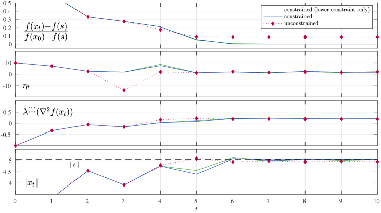
Figure 4: Steepest descent variants applied on $A=\mathop{\rm diag}([-1;-0.8;-0.5])$, $b=[0.04;0.15;0.3]$ and $\rho=0.2$. The red, green, and blue curves correspond to $C_{t}=\mathbb{R}$, $C_{t}=[0,\infty)$ and $C_{t}$ given by (26), respectively.

In Fig. 4, we display the quantities $f(x_{t}),\eta_{t},\lambda^{(1)}(\nabla^{2}f(x_{t}))$, and $\|x_{t}\|$ for the above line-search variants on a $d=3$-dimensional problem instance. The step sizes differ at iteration $t=3$, where the unconstrained gradient step makes almost $50\%$ more progress than steps restricted to be positive. However, it then converges to a sub-optimal local minimum (note $\lambda^{(1)}(\nabla^{2}f(x_{t}))>0$) approximately $9\%$ worse than the global minimum achieved by the guarded sequence (26). The step sizes these methods choose are significantly larger than the $\eta$ Assumption A allows, which is approximately $0.12$. Fig. 4 reveals a difference between fixed step size gradient descent and the line-search schemes—the norm $\left\|{x_{t}}\right\|$ of the line-search-based iterates is non-monotonic and overshoots $\left\|{x_{\star}}\right\|$. Our convergence rate proofs hinge on Lemma 2.6, that $\left\|{x_{t}}\right\|$ is increasing, so extension of our rates to line-search schemes is not straightforward.

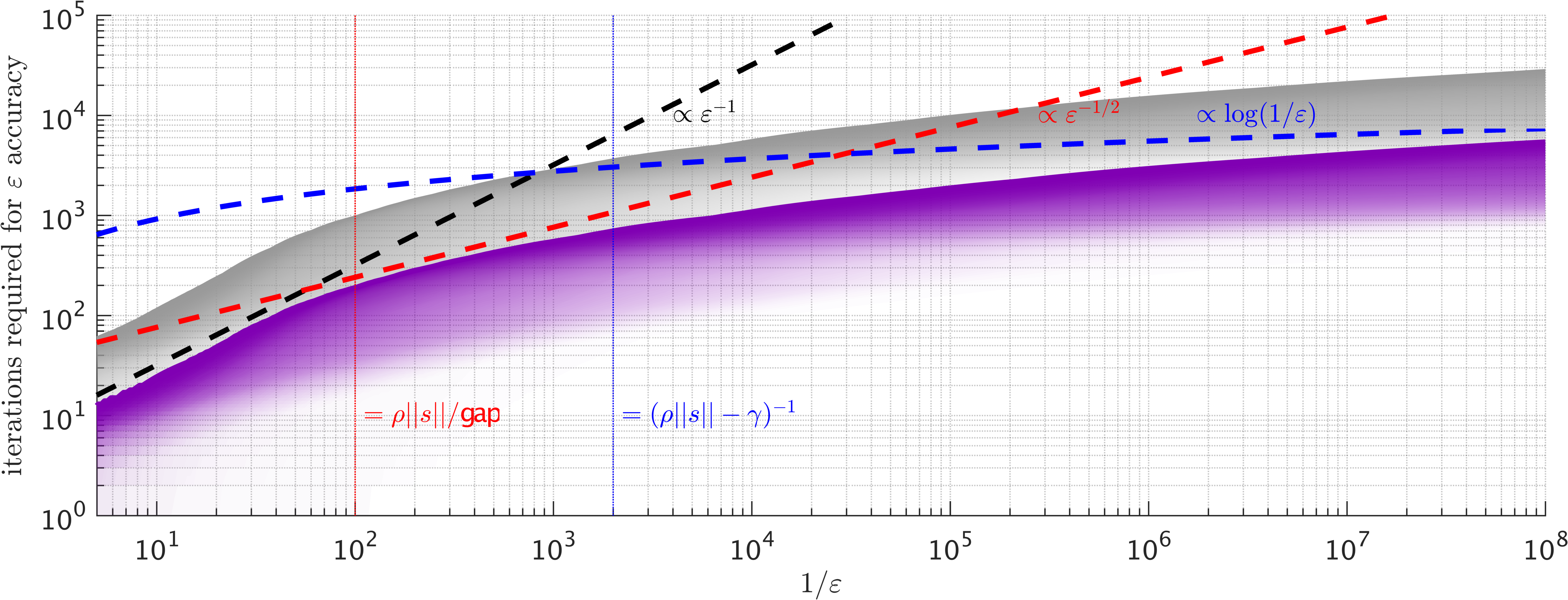
Figure 5: Reproduction of the ensemble experiment reported in Section 3.2 (Figure 3), with the scheme (26) used instead of fixed step size gradient descent. The cdf for fixed step size $\eta=0.25$ is shown in gray for comparison.

We believe that the rate guarantees of Theorem 3.1 apply also to the step size choice (26). To lend credence to this hypothesis, we repeat the ensemble experiment detailed in Section 3.2 (Figure 3), where we use the step size (26) instead of the fixed step size. Figure 5 shows that the rates we prove in Section 3 seem to accurately describe the behavior of guarded steepest descent as well, with constant factors.

We remark that we introduce the upper constraint (26) only because we require it in the proof of Proposition 5.1. Empirically, a scheme with the simpler constraint $C_{t}=[0,\infty)$ appears to converge to the global minimum as well, though we remain unable to prove this. While such step size can differ from the choice (26) (see time $t=4$ in Fig. 4), the variants seem equally practicable. Indeed, we performed the ensemble experiment (Figs. 3 and 5) with $C_{t}=[0,\infty)$ and the results are indistinguishable.

6 Application: A Hessian-free majorization method

In this section we use our main results to analyze a simple optimization scheme that approximates the cubic-regularized Newton steps with gradient descent. We expect more elaborate schemes to be more efficient in practice, as the current procedure is both simplified and uses gradient descent rather than Krylov subspace methods (see the introduction). We believe that our analysis extends to such practical schemes beyond the scope of this paper.

We consider functions $g$ satisfying the following

Assumption C.

The function $g$ satisfies $\inf g\geq\underline{g}>-\infty$, is $\beta$-smooth and has $2\rho$-Lipschitz Hessian, i.e. $\|\nabla^{2}g(y)-\nabla^{2}g(y^{\prime})\|\leq 2\rho\|y-y^{\prime}\|$ for every $y,y^{\prime}\in\mathbb{R}^{d}$.

The first two parts of Assumption C (boundedness and smoothness) are standard. The third implies that $g$ is upper bounded by its cubic-regularized quadratic approximation [25, Lemma 1]: for $y,\Delta\in\mathbb{R}^{d}$ one has

$$g(y+\Delta)\leq g(y)+\nabla g(y)^{T}\Delta+\frac{1}{2}\Delta^{T}\nabla^{2}g(y)\Delta+\frac{\rho}{3}\left\|{\Delta}\right\|^{3}.$$ (27)

For simplicity we assume that the constants $\beta$ and $\rho$ are known. From a theoretical perspective this is a benign assumption, as we may estimate these constants without significantly affecting the complexity bounds [24]. In practice, however, careful adaptive estimation of $\rho$ is crucial for good performance; this is a primary strength of the ARC method [7].

Following  [25, 12], our goal is to find an $\epsilon$-second-order stationary point $y_{\epsilon}$:

$$\left\|{\nabla g(y_{\epsilon})}\right\|\leq\epsilon~{}~{}\textrm{and}~{}~{}\nabla^{2}g(y_{\epsilon})\succeq-\sqrt{\rho\epsilon}I.$$ (28)

Intuitively, $\epsilon$-second-order stationary points provide a finer approximation to local minima than $\epsilon$-stationary points (with only $\left\|{\nabla g(y)}\right\|\leq\epsilon$). Throughout this section, we use $\epsilon$ to denote approximate stationarity in $g$, and continue to use $\varepsilon$ to denote approximate optimality for subproblems of the form (1).

We outline a majorization-minimization strategy [9, 26] for optimization of $g$ in Algorithm 1. At each iteration, the method approximately minimizes a local model of $g$, halting once progress decreasing $g$ falls below a certain threshold. In Algorithm 2, we describe a simple Hessian-free subproblem solver that uses gradient descent with a small perturbation to the linear term and fixed step size (as in Theorem 3.2); we write the method in terms of an input matrix $A=\nabla^{2}g(y)$, noting that it requires only matrix-vector products $Av$ implementable by a first-order oracle for $g$.

The method Solve-subproblem takes as input a problem instance $(A,b,\rho)$, confidence level $\delta$, relative accuracy $\varepsilon^{\prime}$, and a threshold for the magnitude of the global minimizer $x_{\star}$, which we denote by $r$. As an immediate consequence of Theorem 3.2, as long as $\|x_{\star}\|\geq r$ the method is guaranteed to terminate before reaching line 10, and if the gradient is sufficiently large, termination occurs before entering the loop. We formalize this in the following lemma, whose proof we provide in Appendix D.1.

Algorithm 1 A second-order majorization method

1:function Solve-problem($y_{0}$, $g$, $\beta$, $\rho$, $\epsilon$, $\delta$)

2:     Set $K_{\mathrm{prog}}=1/324$ and $\eta=1/(10\beta)$

3:     for $k=1,2,\ldots$ do $\triangleright$ guaranteed to terminate in at most $O(\epsilon^{-3/2})$ iterations

4:         $\Delta_{k}\leftarrow\hyperref@@ii[func:SSP]{\textsc{Solve-subproblem}(\nabla^{2}g(y_{k-1}),\ \nabla g(y_{k-1}),\ \rho,\ \eta,\ \sqrt{\frac{\epsilon}{9\rho}},\ \frac{1}{2},\ \frac{\delta}{2k^{2}})}$

5:         if  $g(y_{k-1}+\Delta_{k})\leq g(y_{k})-K_{\mathrm{prog}}\epsilon^{3/2}\rho^{-1/2}$ then

6:              $y_{k}\leftarrow y_{k-1}+\Delta_{k}$

7:         else

8:              $\Delta_{k}\leftarrow\hyperref@@ii[func:SFSP]{\textsc{Solve-final-subproblem}(\nabla^{2}g(y_{k-1}),\ \nabla g(y_{k-1}),\ \rho,\ \eta,\ \frac{\epsilon}{2})}$

9:              return $y_{k-1}+\Delta_{k}$               

Algorithm 2 A Hessian-free subproblem solver

1:function Solve-subproblem($A$, $b$, $\rho$, $\eta$, $r$, $\varepsilon^{\prime}$, $\delta$)

2:     Set $f(x)=(1/2)x^{T}Ax+b^{T}x+(\rho/3)\|x\|^{3}$ and $x_{0}=\hyperref@@ii[func:CP]{\textsc{Cauchy-point}(A,b,\rho)}$

3:     if $f(x_{0})\leq-(1-\varepsilon^{\prime})\rho r^{3}/6$ then return $x_{0}$      

4:     Set

$$T=\frac{480}{\eta\rho r\varepsilon^{\prime}}\bigg{[}6\log\bigg{(}1+\frac{\sqrt{d}}{\delta}\bigg{)}+44\log\left(\frac{6}{\eta\rho r\varepsilon^{\prime}}\right)\bigg{]}$$

5:     Set $\sigma=\frac{\rho^{3}r^{4}(\varepsilon^{\prime})^{2}}{2(120\beta+240\rho r)^{2}}$, draw $q$ uniformly from the unit sphere, set $\tilde{b}=b+\sigma q$

6:     Set $\tilde{f}(x)=(1/2)x^{T}Ax+\tilde{b}^{T}x+(\rho/3)\|x\|^{3}$ and $\tilde{x}_{0}=\hyperref@@ii[func:CP]{\textsc{Cauchy-point}(A,\tilde{b},\rho)}$

7:     for $t=1,2,\ldots,T$ do

8:         $\tilde{x}_{t}\leftarrow\tilde{x}_{t-1}-\eta\nabla\tilde{f}(\tilde{x}_{t-1})$

9:         if $f(\tilde{x}_{t})\leq-(1-\varepsilon^{\prime})\rho r^{3}/6$ then return $\tilde{x}_{t}$               

10:     return $\tilde{x}_{t}$

1:function Solve-final-subproblem($A$, $b$, $\rho$, $\eta$, $\varepsilon_{\mathrm{g}}$)

2:     Set $f(x)=(1/2)x^{T}Ax+b^{T}x+(\rho/3)\|x\|^{3}$ and $\Delta=\hyperref@@ii[func:CP]{\textsc{Cauchy-point}(A,b,\rho)}$

3:     while $\left\|{\nabla f(\Delta)}\right\|>\varepsilon_{\mathrm{g}}$ do $\Delta\leftarrow\Delta-\eta\nabla f(\Delta)$      

4:     return $\Delta$

1:function Cauchy-point($A$, $b$, $\rho$)

2:     return $-R_{c}b/\left\|{b}\right\|$ where $R_{c}=\frac{-b^{T}Ab}{2\rho\|b\|^{2}}+\sqrt{\left(\frac{b^{T}Ab}{2\rho\|b\|^{2}}\right)^{2}+\frac{\|b\|}{\rho}}$

Lemma 6.1.

Let $A\in\mathbb{R}^{d\times d}$ satisfy $\left\|{A}\right\|_{2}\leq\beta$, $b\in\mathbb{R}^{d}$, $\rho>0,r>0$, $\varepsilon^{\prime}\in(0,1),\delta\in(0,1)$ and $\eta\leq 1/(8\beta+4\rho r)$. With probability at least $1-\delta$, if

$$\|x_{\star}\|\geq r\textrm{ or }\|b\|\geq\max\{\sqrt{\beta\rho}r^{3/2},\rho r^{2}\}$$

then $x=\text{\hyperref@@ii[func:SSP]{{Solve-subproblem}($A$, $b$, $\rho$, $\eta$, $r$, $\varepsilon^{\prime}$, $\delta$)}}$ satisfies $f(x)\leq(1-\varepsilon^{\prime})\rho r^{3}/6$.

Let $\Delta^{\star}_{k}$ be the global minimizer (in $\Delta$) of the model (27) at $y=y_{k}$, the $k$th iterate of Algorithm 1. Lemma 6.1 guarantees that with high probability, if Solve-subproblem fails to meet the progress condition in line 5 at iteration $k$, then $\|\Delta^{\star}_{k}\|\leq\sqrt{\epsilon/(9\rho)}$, and therefore $\lambda^{(1)}(\nabla^{2}g(y_{k}))\geq-\rho\|\Delta^{\star}_{k}\|\geq-\sqrt{\rho\epsilon}$. It is possible, nonetheless, that $\left\|{\nabla g(y_{k})}\right\|>\epsilon$; to address this, we correctively apply gradient descent on the final subproblem (Solve-final-subproblem).

Building off of an argument of Nesterov and Polyak [25, Lemma 5], we obtain the following guarantee for Algorithm 1, whose proof we provide in Appendix D.2.

Proposition 6.2.

Let $g$ satisfy Assumption C, $y_{0}\in\mathbb{R}^{d}$ be arbitrary, and let $\delta\in(0,1]$ and $\epsilon\leq\min\{\beta^{2}/\rho,\rho^{1/3}(g(y_{0})-\underline{g})^{2/3}\}$. With probability at least $1-\delta$, Algorithm 1 finds an $\epsilon$-second-order stationary point (28) in at most

$$O(1)\cdot\frac{\beta(g(y_{0})-\underline{g})}{\epsilon^{2}}\log\left(\frac{d}{\delta}\cdot\frac{\beta(g(y_{0})-\underline{g})}{\epsilon^{2}}\right)$$ (29)

Hessian-vector product evaluations, and at most

$$O(1)\cdot\frac{\sqrt{\rho}(g(y_{0})-\underline{g})}{\epsilon^{3/2}}$$

calls to Solve-subproblem and gradient evaluations.

In Proposition 6.2, the assumption $\epsilon\leq\beta^{2}/\rho$ is no loss of generality, as otherwise the Hessian guarantee (28) is trivial, and we may obtain the gradient guarantee by simply running gradient descent on $g$ for $2\beta(g(y_{0})-\underline{g})\epsilon^{-2}$ iterations. Similarly, if $\epsilon>\rho^{1/3}(g(y_{0})-\underline{g})^{2/3}$ then we require at most $1+1/K_{\mathrm{prog}}=325$ calls to Solve-subproblem, and the proof of Proposition 6.2 reveals that the overall first-order complexity scales as $\epsilon^{-1/2}$ instead of $\epsilon^{-2}$.

There are other Hessian-free methods that provide the guarantee (28), and recent schemes using acceleration techniques [1, 5] provide it in roughly $\epsilon^{-7/4}\log\frac{d}{\delta}$ first-order operations, which is better than Algorithm 1. Nevertheless, this section illustrates how gradient descent on the structured problem (1) can be straightforwardly leveraged to optimize general smooth non-convex functions.

7 Discussion

Our results have a number of connections to rates of convergence in classical (smooth) convex optimization and the power method for symmetric eigenvector computation; here, we explore these in more detail.

7.1 Comparison with convex optimization

For $L$-smooth $\alpha$-strongly convex functions, gradient descent finds an $\varepsilon$-suboptimal point within

$$O(1)\cdot\min\left\{\frac{L}{\alpha}\log\frac{LD^{2}}{\varepsilon},\frac{LD^{2}}{\varepsilon}\right\}$$

iterations [23], where $D$ is any constant $D\geq\left\|{x_{0}-x^{\star}}\right\|$ and $x^{\star}$ a global minimizer. For our (possibly non-convex) problem (1), Corollary 3.3 guarantees that gradient descent finds an $\varepsilon$-suboptimal point (with probability at least $1-\delta$) within

$$O(1)\cdot\min\left\{\frac{L_{\star}}{\rho\left\|{x_{\star}}\right\|-\gamma},\frac{L_{\star}\left\|{x_{\star}}\right\|^{2}}{\varepsilon}\right\}\left[\log\frac{L_{\star}\left\|{x_{\star}}\right\|^{2}}{\varepsilon}+\log\left(1+\mathbb{I}_{\{\gamma>0\}}\frac{d}{\delta}\right)\right]$$

iterations, where $L_{\star}=\beta+2\rho\left\|{x_{\star}}\right\|$. The parallels are immediate: by Lemma 2.6, $L_{\star}$ and $\left\|{x_{\star}}\right\|$ are precise analogues of $L$ and $D$ in the convex setting. Moreover, the quantity $\rho\left\|{x_{\star}}\right\|-\gamma$ plays the role of the strong convexity parameter $\alpha$, but it is well-defined even when $f$ is not convex. When $\lambda^{\left({1}\right)}(A)=-\gamma\geq 0$, $f$ is $-\gamma$-strongly convex, and because $\rho\left\|{x_{\star}}\right\|-\gamma>-\gamma$, our analysis for the cubic problem (1) guarantees better conditioning than the generic convex result. The difference between $\rho\left\|{x_{\star}}\right\|-\gamma$ and $-\gamma$ becomes significant when $b$ is sufficiently large, as we observe from the bounds (7b) and (8). Even in the non-convex case that $\gamma>0$, gradient descent still exhibits linear convergence whenever high accuracy is desired, that is, when $\varepsilon/\left\|{x_{\star}}\right\|^{2}\leq\rho\left\|{x_{\star}}\right\|-\gamma$.

When $\gamma>0$, our guarantee becomes probabilistic and contains a $\log(d/\delta)$ term. Such a term does not appear in results on convex optimization [23], and it is fundamentally related to the presence of saddle-points in the objective [30].

7.2 Comparison with the power method

The power method for finding the smallest eigenvector of $A$ is the recursion $x_{t+1}=(I-(1/\beta)A)x_{t}/\|(I-(1/\beta)A)x_{t}\|$ where $x_{0}$ is uniform on the unit sphere [17, 21]. This method guarantees that with probability at least $1-\delta$, $x_{t}^{T}Ax_{t}\leq-\gamma+\varepsilon$ for all

$$t\geq O(1)\cdot\min\left\{\frac{\beta}{\varepsilon}\log\left(\frac{d}{\delta}\right),\frac{\beta}{\mathsf{gap}}\log\left(\frac{\beta}{\varepsilon}\cdot\frac{d}{\delta}\right)\right\}.$$

When $b=0$ and $\lambda^{\left({1}\right)}(A)=-\gamma<0$, any global minimizer of problem (1) is an eigenvector of $A$ with eigenvalue $-\gamma$ and $\rho\left\|{x_{\star}}\right\|=\gamma$, so it is natural to compare gradient descent and the power method. For simplicity, let us assume that $\rho=\gamma$ so that $\left\|{x_{\star}}\right\|=1$, and both methods converge to unit eigenvectors. Under these assumptions $f(x)=\frac{1}{2}x^{T}Ax+\frac{\gamma}{3}\left\|{x}\right\|^{3}$ and $f(x_{\star})=-\gamma/6$, so $f(x)\leq f(x_{\star})+\varepsilon^{\prime}$ implies

$$\frac{x^{T}Ax}{\left\|{x}\right\|^{2}}\leq-\frac{\gamma}{3}\left[\frac{1}{\left\|{x}\right\|^{2}}+2\left\|{x}\right\|\right]+\frac{2\varepsilon^{\prime}}{\left\|{x}\right\|^{2}}\leq-\gamma+\frac{2\varepsilon^{\prime}}{\left\|{x}\right\|^{2}}.$$

Consider gradient descent applied to $f$ with a random perturbation as described in Theorem 3.2, with $\overline{\sigma}=1$. Inspecting the proofs of our theorems (Sec. 4), we see that Lemmas 4.3 and 4.6 imply that with probability at least $1-\delta$ we have $\left\|{\tilde{x}_{t}}\right\|\geq 1/2$ for every $t\geq O(1)\log(\frac{L_{\star}\left\|{x_{\star}}\right\|^{2}}{\varepsilon}\cdot\frac{d}{\delta})$. As in Corollary 3.3, setting $\eta=\frac{1}{4(\beta+\rho R)}=\frac{1}{8\beta}$ guarantees that with probability at least $1-\delta$, $\tilde{x}_{t}^{T}A\tilde{x}_{t}/\left\|{\tilde{x}_{t}}\right\|^{2}\leq-\gamma+\varepsilon$ for all

$$t\geq O(1)\cdot\min\left\{\frac{\beta}{\varepsilon}\log\left(\frac{\beta}{\varepsilon}\cdot\frac{d}{\delta}\right),\frac{\beta}{\sqrt{\varepsilon\min\{\mathsf{gap},\gamma\}}}\log\left(\frac{\beta}{\varepsilon}\cdot\frac{d}{\delta}\right)\right\}.$$

Comparing the rates of convergence, we see that both exhibit the $\log(d/\delta)$ hallmark of non-convexity and gap-free and gap-dependent convergence regimes. Of course, the power method also finds eigenvectors when $\gamma<0$, while the unique solution to problem (1) when $b=0$ and $\gamma<0$ is simply $x_{\star}=0$. In the gap-dependent regime, however, the power method enjoys linear convergence when $\varepsilon<\mathsf{gap}$, while our bounds have a $1/\sqrt{\varepsilon}$ factor. Although this may be due to looseness in our analysis, we suspect it is real and related to the fact that gradient descent needs to “grow” the iterates to have norm $\left\|{x_{t}}\right\|\approx\gamma_{+}/\rho$, while the power method iterates always have unit norm. If one is only interested in finding eigenvectors of $A$, there is probably no reason to prefer the cubic-regularized objective to the power method.

Appendix

For convenience of the reader, throughout the appendix we restate lemmas that appeared in the main text prior to giving their proofs.

Appendix A Proof of Lemma 2.3

Before proving Lemma 2.3, we state and prove two technical lemmas (see Sec. A.1 for the proof conditional on these lemmas). For the first lemma, let $\kappa\in\mathbb{R}^{d}$ satisfy $\kappa^{\left({1}\right)}\leq\kappa^{\left({2}\right)}\leq\ldots\leq\kappa^{\left({d}\right)}$, let $\nu_{t}$ be a nonnegative and nondecreasing sequence, $0\leq\nu_{1}\leq\nu_{2}\leq\ldots$, and consider the process

$$z_{t}^{\left({i}\right)}=(1-\kappa^{\left({i}\right)}-\nu_{t-1})z_{t-1}^{\left({i}\right)}+1.$$ (30)

Additionally, assume $1-\kappa^{\left({i}\right)}-\nu_{t-1}\geq 0$ for all $i$ and $t$.

Lemma A.1.

Let $z_{0}^{\left({i}\right)}=c_{0}\geq 0$ for every $i\in[d]$. Then for every $t\in\mathbb{N}$ and $j\in[d]$, the following holds.

1. If $z_{t}^{\left(j\right)}\leq z_{t-1}^{\left(j\right)}$ then also $z_{t^{\prime}}^{\left(j\right)}\leq z_{t^{\prime}-1}^{\left(j\right)}$ for every $t^{\prime}>t$.

2. If $z_{t}^{\left(j\right)}\geq z_{t-1}^{\left(j\right)}$, then $z_{t}^{\left(j\right)}/z_{t+1}^{\left(j\right)}\geq z_{t}^{\left({i}\right)}/z_{t+1}^{\left({i}\right)}$ for every $i\leq j$.

3. If $z_{t+1}^{\left({i}\right)}\leq z_{t}^{\left({i}\right)}$, then $z_{t+1}^{\left({j}\right)}\leq z_{t}^{\left({j}\right)}$ for every $j\geq i$.

Proof.    For shorthand, we define $\delta_{t}^{\left({i}\right)}\triangleq\kappa^{\left({i}\right)}+\nu_{t}$.

We first establish part (i) of the lemma. By (30), we have

$$z_{t+1}^{\left({j}\right)}-z_{t}^{\left({j}\right)}=(1-\delta_{t-1}^{\left(j\right)})(z_{t}^{\left(j\right)}-z_{t-1}^{\left(j\right)})-(\delta_{t}^{\left(j\right)}-\delta_{t-1}^{\left(j\right)})z_{t}^{\left(j\right)}$$

By our assumptions that $z_{0}^{\left({j}\right)}\geq 0$ and that $1-\delta_{t}^{\left({j}\right)}\geq 0$ for every $t$ we immediately have that $z_{t}^{\left({j}\right)}\geq 0$, and therefore also $(\delta_{t}^{\left({j}\right)}-\delta_{t-1}^{\left({j}\right)})z_{t}^{\left({j}\right)}=(\nu_{t}-\nu_{t-1})z_{t}^{\left({j}\right)}\geq 0$. We therefore conclude that

$$z_{t+1}^{\left({j}\right)}-z_{t}^{\left({j}\right)}\leq(1-\delta_{t-1}^{\left({j}\right)})(z_{t}^{\left({j}\right)}-z_{t-1}^{\left({j}\right)})\leq 0,$$

and induction gives part (i).

To establish part (ii) of the lemma, first note that by the contrapositive of part (i), $z_{t}^{\left({j}\right)}\geq z_{t-1}^{\left({j}\right)}$ for some $t$ implies $z_{t^{\prime}}^{\left({j}\right)}\geq z_{t^{\prime}-1}^{\left({j}\right)}$ for any $t^{\prime}\leq t$. We prove by induction that

$$z_{t^{\prime}}^{\left({i}\right)}-z_{t^{\prime}}^{\left({j}\right)}\leq(\kappa^{\left({j}\right)}-\kappa^{\left({i}\right)})z_{t^{\prime}}^{\left({i}\right)}z_{t^{\prime}}^{\left({j}\right)}$$ (31)

for any $i\leq j$ and $t^{\prime}\leq t$. The basis of the induction is immediate from the assumption $z_{0}^{\left({i}\right)}=z_{0}^{\left({j}\right)}\geq 0$. Assuming the property holds through time $t^{\prime}-1$ for $t^{\prime}\leq t$, we obtain

$$\frac{z_{t^{\prime}}^{\left({i}\right)}-z_{t^{\prime}}^{\left({j}\right)}}{z_{t^{\prime}}^{\left({i}\right)}z_{t^{\prime}}^{\left({j}\right)}} =\frac{(1-\delta_{t^{\prime}-1}^{\left({i}\right)})(z_{t^{\prime}-1}^{\left({i}\right)}-z_{t^{\prime}-1}^{\left({j}\right)})+(\delta_{t^{\prime}-1}^{\left({j}\right)}-\delta_{t^{\prime}-1}^{\left({i}\right)})z_{t^{\prime}-1}^{\left({j}\right)}}{z_{t^{\prime}}^{\left({i}\right)}z_{t^{\prime}}^{\left({j}\right)}}$$

$$\leq\frac{(1-\delta_{t^{\prime}-1}^{\left({i}\right)})(\kappa^{\left({j}\right)}-\kappa^{\left({i}\right)})z_{t^{\prime}-1}^{\left({i}\right)}z_{t^{\prime}-1}^{\left({j}\right)}}{z_{t^{\prime}}^{\left({i}\right)}z_{t^{\prime}}^{\left({j}\right)}}=(\kappa^{\left({j}\right)}-\kappa^{\left({i}\right)})\frac{z_{t^{\prime}-1}^{\left({j}\right)}}{z_{t^{\prime}}^{\left({j}\right)}}\leq\kappa^{\left({j}\right)}-\kappa^{\left({i}\right)}$$

where the first inequality uses inequality (31) (assumed by induction) and the second uses $z_{t^{\prime}-1}^{\left({j}\right)}\leq z_{t^{\prime}}^{\left({j}\right)}$ for any $t^{\prime}\leq t$, as argued above. With the bound $z_{t}^{\left({i}\right)}-z_{t}^{\left({j}\right)}\leq(\kappa^{\left({j}\right)}-\kappa^{\left({i}\right)})z_{t}^{\left({i}\right)}z_{t}^{\left({j}\right)}$ in place, we may finish the proof of part (ii) by noting that

$$\frac{z_{t}^{\left({j}\right)}}{z_{t+1}^{\left({j}\right)}}-\frac{z_{t}^{\left({i}\right)}}{z_{t+1}^{\left({i}\right)}} =\frac{z_{t+1}^{\left({i}\right)}z_{t}^{\left({j}\right)}-z_{t+1}^{\left({j}\right)}z_{t}^{\left({i}\right)}}{z_{t+1}^{\left({j}\right)}z_{t+1}^{\left({i}\right)}}=\frac{(\kappa^{\left({j}\right)}-\kappa^{\left({i}\right)})z_{t}^{\left({i}\right)}z_{t}^{\left({j}\right)}-(z_{t}^{\left({i}\right)}-z_{t}^{\left({j}\right)})}{z_{t+1}^{\left({j}\right)}z_{t+1}^{\left({i}\right)}}\geq 0.$$

Lastly, we prove part (iii). If $z_{t}^{\left({j}\right)}\leq z_{t-1}^{\left({j}\right)}$ then we have $z_{t+1}^{\left({j}\right)}\leq z_{t}^{\left({j}\right)}$ by part (i). Otherwise we have $z_{t}^{\left({j}\right)}\geq z_{t-1}^{\left({j}\right)}$, and so $z_{t}^{\left({j}\right)}/z_{t+1}^{\left({j}\right)}\geq z_{t}^{\left({i}\right)}/z_{t+1}^{\left({i}\right)}$ by part (ii). As $z_{t+1}^{\left({i}\right)}\leq z_{t}^{\left({i}\right)}$, this implies $z_{t}^{\left({j}\right)}/z_{t+1}^{\left({j}\right)}\geq z_{t}^{\left({i}\right)}/z_{t+1}^{\left({i}\right)}\geq 1$ and therefore $z_{t+1}^{\left({j}\right)}\leq z_{t}^{\left({j}\right)}$ as required. ∎

Our second technical lemma provides a lower bound on certain inner products in the gradient descent iterations. In the lemma, we recall the definition (7a) of $R$.

Lemma A.2.

Assume that $\left\|{x_{\tau}}\right\|$ is non-decreasing in $\tau$ for $\tau\leq t$, that $\left\|{x_{t}}\right\|\leq R$, and that $x_{t}^{T}\nabla f(x_{t})\leq 0$. Then $x_{t}^{T}A\nabla f(x_{t})\geq\beta x_{t}^{T}\nabla f(x_{t})$.

Proof.    If we define $z_{t}^{\left({i}\right)}=x_{t}^{\left({i}\right)}/(-\eta b^{\left({i}\right)})$, then evidently

$$z_{t+1}^{\left({i}\right)}=(1-\underset{\triangleq\kappa^{\left({i}\right)}}{\underbrace{\eta\lambda^{\left({i}\right)}\left(A\right)}}-\underset{\triangleq\nu_{t}}{\underbrace{\eta\rho\left\|{x_{t}}\right\|}})z_{t}^{\left({i}\right)}+1.$$

We verify that $z_{t}^{\left({i}\right)}$ satisfies the conditions of Lemma A.1:

1. By definition $\kappa^{\left({i}\right)}$ are increasing in $i$, and $\nu_{0}\leq\nu_{1}\leq\cdots\leq\nu_{t}$ by our assumption that $\left\|{x_{\tau}}\right\|$ is non-decreasing for $\tau\leq t$.

2. As $\eta\leq 1/\left(\beta+\rho R\right)$ for $\tau\leq t$, we have that $\kappa^{\left({i}\right)}+\nu_{\tau}\leq 1$ for $\tau\leq t$ and $i\in[d]$.

3. As $x_{0}=-rb/\left\|{b}\right\|$, $z_{0}^{\left({i}\right)}=r/(\eta\left\|{b}\right\|)\geq 0$ for every $i$.

We may therefore apply Lemma A.1, part (iii) to conclude that $z_{t}^{\left({i}\right)}-z_{t+1}^{\left({i}\right)}\geq 0$ implies $z_{t}^{\left({j}\right)}-z_{t+1}^{\left({j}\right)}\geq 0$ for every $j\geq i$. Since $z_{t}^{\left({i}\right)}\geq 0$ for every $i$,

$$\mathrm{sign}\left(x_{t}^{\left({i}\right)}\left(x_{t}^{\left({i}\right)}-x_{t+1}^{\left({i}\right)}\right)\right)=\mathrm{sign}\left(z_{t}^{\left({i}\right)}\left(z_{t}^{\left({i}\right)}-z_{t+1}^{\left({i}\right)}\right)\right)=\mathrm{sign}\left(z_{t}^{\left({i}\right)}-z_{t+1}^{\left({i}\right)}\right),$$

and there must thus exist some $i^{*}\in[d]$ such that $x_{t}^{\left({i}\right)}(x_{t}^{\left({i}\right)}-x_{t+1}^{\left({i}\right)})\leq 0$ for every $i\leq i^{*}$ and $x_{t}^{\left({i}\right)}(x_{t}^{\left({i}\right)}-x_{t+1}^{\left({i}\right)})\geq 0$ for every $i>i^{*}$. We thus have (by expanding in the eigenbasis of $A$) that

$$x_{t}^{T}A\nabla f\left(x_{t}\right)=\frac{1}{\eta}\sum_{i=1}^{i^{*}}\lambda^{\left({i}\right)}\left(A\right)x_{t}^{\left({i}\right)}\left(x_{t}^{\left({i}\right)}-x_{t+1}^{\left({i}\right)}\right)+\frac{1}{\eta}\sum_{i=i^{*}+1}^{d}\lambda^{\left({i}\right)}\left(A\right)x_{t}^{\left({i}\right)}\left(x_{t}^{\left({i}\right)}-x_{t+1}^{\left({i}\right)}\right)$$

$$\quad\geq\lambda^{\left(i^{*}\right)}\left(A\right)\frac{1}{\eta}\sum_{i=1}^{i^{*}}x_{t}^{\left({i}\right)}\left(x_{t}^{\left({i}\right)}-x_{t+1}^{\left({i}\right)}\right)+\lambda^{\left(i^{*}+1\right)}\left(A\right)\frac{1}{\eta}\sum_{i=i^{*}+1}^{d}x_{t}^{\left({i}\right)}\left(x_{t}^{\left({i}\right)}-x_{t+1}^{\left({i}\right)}\right)$$

$$\quad\geq\lambda^{\left(i^{*}\right)}\left(A\right)\frac{1}{\eta}\sum_{i=1}^{d}x_{t}^{\left({i}\right)}\left(x_{t}^{\left({i}\right)}-x_{t+1}^{\left({i}\right)}\right)=\lambda^{\left(i^{*}\right)}\left(A\right)x_{t}^{T}\nabla f\left(x_{t}\right)\geq\beta x_{t}^{T}\nabla f\left(x_{t}\right)$$

where the first two inequalities use the fact the $\lambda^{\left({i}\right)}$ is non-decreasing with $i$, and the last inequality uses our assumption that $x_{t}^{T}\nabla f\left(x_{t}\right)\leq 0$ along with $\lambda^{\left(d\right)}\left(A\right)\leq\beta$. ∎

A.1 Proof of Lemma 2.3

See 2.3

By definition of the gradient descent iteration, we have

$$\left\|{x_{t+1}}\right\|^{2}=\left\|{x_{t}}\right\|^{2}-2\eta x_{t}^{T}\nabla f\left(x_{t}\right)+\eta^{2}\left\|{\nabla f\left(x_{t}\right)}\right\|^{2},$$ (32)

and therefore if we can show that $x_{t}^{T}\nabla f\left(x_{t}\right)\leq 0$ for all $t$, the lemma holds. We give a proof by induction. The basis of the induction $x_{0}^{T}\nabla f\left(x_{0}\right)\leq 0$ is immediate as $r\mapsto f(-rb/\left\|{b}\right\|)$ is decreasing until $r=R_{c}$ (recall the definition (8)), and $x_{0}^{T}\nabla f(x_{0})=0$ for $r\in\{0,R_{c}\}$. Our induction assumption is that $x_{t^{\prime}-1}^{T}\nabla f\left(x_{t^{\prime}-1}\right)\leq 0$ (and hence also $\left\|{x_{t^{\prime}}}\right\|\geq\left\|{x_{t^{\prime}-1}}\right\|$) for $t^{\prime}\leq t$ and we wish to show that $x_{t}^{T}\nabla f\left(x_{t}\right)\leq 0$. Note that

$$x^{T}\nabla f\left(x\right)=x^{T}Ax+\rho\left\|{x}\right\|^{3}+b^{T}x\geq\rho\left\|{x}\right\|^{3}-\gamma\left\|{x}\right\|^{2}-\left\|{b}\right\|\left\|{x}\right\|$$

and therefore $x^{T}\nabla f\left(x\right)>0$ for every $\left\|{x}\right\|>R_{\rm low}\triangleq\frac{\gamma}{2\rho}+\sqrt{\left(\frac{\gamma}{2\rho}\right)^{2}+\frac{\left\|{b}\right\|}{\rho}}$. Therefore, our induction assumption also implies $\left\|{x_{t^{\prime}-1}}\right\|\leq R_{\rm low}\leq R$ for every $t^{\prime}\leq t$.

Using that $\nabla^{2}f$ is $2\rho$-Lipschitz, a Taylor expansion immediately implies [25, Lemma 1] that for all vectors $\Delta$, we have

$$\left\|{\nabla f(x+\Delta)-(\nabla f(x)+\nabla^{2}f(x)\Delta)}\right\|\leq\rho\left\|{\Delta}\right\|^{2}.$$ (33)

Thus, if we define $\Delta_{t}\triangleq\frac{1}{\eta^{2}}[\nabla f(x_{t})-(\nabla f(x_{t-1})-\eta\nabla^{2}f(x_{t-1})\nabla f(x_{t-1}))]$, we have $\left\|{\Delta_{t}}\right\|\leq\rho\left\|{\nabla f(x_{t-1})}\right\|^{2}$, and using the iteration $x_{t}=x_{t-1}-\eta\nabla f(x_{t-1})$ yields

$$x_{t}^{T}\nabla f\left(x_{t}\right) =x_{t-1}^{T}\nabla f\left(x_{t-1}\right)-\eta\left\|{\nabla f\left(x_{t-1}\right)}\right\|^{2}-\eta\underbrace{x_{t-1}^{T}\nabla^{2}f\left(x_{t-1}\right)\nabla f\left(x_{t-1}\right)}_{\triangleq\mathcal{T}_{1}}$$

$$\qquad+\eta^{2}\underbrace{\nabla f\left(x_{t-1}\right)^{T}\nabla^{2}f\left(x_{t-1}\right)\nabla f\left(x_{t-1}\right)}_{\triangleq\mathcal{T}_{2}}+\eta^{2}\underbrace{x_{t}^{T}\Delta_{t}}_{\triangleq\mathcal{T}_{3}}.$$ (34)

We bound each of the terms $\mathcal{T}_{i}$ in turn. We have that

$$\mathcal{T}_{1} =x_{t-1}^{T}\nabla^{2}f\left(x_{t-1}\right)\nabla f\left(x_{t-1}\right)=x_{t-1}^{T}A\nabla f\left(x_{t-1}\right)+2\rho\left\|{x_{t-1}}\right\|x_{t-1}^{T}\nabla f\left(x_{t-1}\right)$$

$$\qquad\geq(\beta+2\rho\left\|{x_{t-1}}\right\|)x_{t-1}^{T}\nabla f(x_{t-1})\geq(\beta+2\rho R)x_{t-1}^{T}\nabla f(x_{t-1}),$$

where both inequalities follow from the induction assumption; the first is Lemma A.2 and the second is due to $\left\|{x_{t-1}}\right\|\leq R$ and $x_{t-1}^{T}\nabla f(x_{t-1})\leq 0$.

Treating the second order term $\mathcal{T}_{2}$, we obtain that

$$\mathcal{T}_{2}\leq\left\|{\nabla^{2}f(x_{t-1})}\right\|_{2}\left\|{\nabla f(x_{t-1})}\right\|^{2}\leq\left(\beta+2\rho R\right)\left\|{\nabla f\left(x_{t-1}\right)}\right\|^{2},$$

and, by the Lipschitz bound (33), the remainder term $\mathcal{T}_{3}$ satisfies

$$\mathcal{T}_{3}=x_{t}^{T}\Delta_{t} \leq\left\|{x_{t}}\right\|\left\|{r}\right\|\leq\rho\left\|{x_{t}}\right\|\left\|{\nabla f\left(x_{t-1}\right)}\right\|^{2}\leq\rho\left\|{x_{t-1}-\eta\nabla f\left(x_{t-1}\right)}\right\|\left\|{\nabla f\left(x_{t-1}\right)}\right\|^{2}$$

$$\leq\rho\left\|{x_{t-1}}\right\|\left\|{\nabla f\left(x_{t-1}\right)}\right\|^{2}+\rho\eta\left\|{\nabla f\left(x_{t-1}\right)}\right\|^{3}.$$

Using that $\left\|{\nabla f(x)}\right\|=\left\|{\nabla f(x)-\nabla f(x_{\star})}\right\|\leq(\beta+2R)\left\|{x-x_{\star}}\right\|\leq R(\beta+2\rho R)$ for $\left\|{x}\right\|\leq R$ and that $\eta\leq 1/2\left(\beta+2\rho R\right)$, our inductive assumption that $\left\|{x_{t-1}}\right\|\leq R$ thus guarantees that $\mathcal{T}_{3}\leq 2\rho R\left\|{\nabla f(x_{t-1})}\right\|^{2}$. Combining our bounds on the terms $\mathcal{T}_{i}$ in expression (34), we have that

$$x_{t}^{T}\nabla f\left(x_{t}\right)\leq\left(1-\eta\left(\beta+2\rho R\right)\right)x_{t-1}^{T}\nabla f\left(x_{t-1}\right)-\left(\eta-\eta^{2}(\beta+4\rho R)\right)\left\|{\nabla f(x_{t-1})}\right\|^{2}.$$

Using $\eta\leq 1/\left(\beta+4\rho R\right)$ shows that $x_{t}^{T}\nabla f\left(x_{t}\right)\leq 0$, completing our induction. By the expansion (32), we have $\left\|{x_{t}}\right\|\leq\left\|{x_{t+1}}\right\|$ as desired, and that $x_{t}^{T}\nabla f(x_{t})\leq 0$ for all $t$ guarantees that $\left\|{x_{t}}\right\|\leq R_{\rm low}\leq R$.

Appendix B Proofs of technical results from Section 4

As in the statement of our major theorems and as we note in the beginning of Section 4, we tacitly assume Assumptions A and B throughout this section.

B.1 Proof of Lemma 4.1

See 4.1

Expanding $x_{t}=x_{t-1}-\eta\nabla f(x_{t-1})$, we have

$$\left\|{x_{t}-x_{\star}}\right\|^{2}=\left\|{x_{t-1}-x_{\star}}\right\|^{2}-2\eta\left(x_{t-1}-x_{\star}\right)^{T}\nabla f(x_{t-1})+\eta^{2}\left\|{\nabla f\left(x_{t-1}\right)}\right\|^{2}.$$ (35)

Using the equality $\nabla f\left(x\right)=A_{\star}\left(x-x_{\star}\right)-\rho\left(\left\|{x_{\star}}\right\|-\left\|{x}\right\|\right)x$, we rewrite the cross-term $\left(x_{t-1}-x_{\star}\right)^{T}\nabla f\left(x_{t-1}\right)$ as

$$\left(x_{t-1}-x_{\star}\right)^{T} A_{\star}\left(x_{t-1}-x_{\star}\right)+\rho\left(\left\|{x_{t-1}}\right\|-\left\|{x_{\star}}\right\|\right)(\left\|{x_{t-1}}\right\|^{2}-x_{\star}^{T}x_{t-1})$$

$$= \left(x_{t-1}-x_{\star}\right)^{T}\left(A_{\star}+\frac{\rho}{2}\left(\left\|{x_{t-1}}\right\|-\left\|{x_{\star}}\right\|\right)I\right)\left(x_{t-1}-x_{\star}\right)$$

$$+\frac{\rho}{2}\left(\left\|{x_{\star}}\right\|-\left\|{x_{t-1}}\right\|\right)^{2}\left(\left\|{x_{t-1}}\right\|+\left\|{x_{\star}}\right\|\right).$$ (36)

Moving to the second order term $\left\|{\nabla f\left(x_{t-1}\right)}\right\|^{2}$ from the expansion (35), we find

$$\left\|{\nabla f\left(x_{t-1}\right)}\right\|^{2} =\left\|{A_{\star}\left(x_{t-1}-x_{\star}\right)+\rho\left(\left\|{x_{t-1}}\right\|-\left\|{x_{\star}}\right\|\right)x_{t-1}}\right\|^{2}$$

$$\leq 2\left(x_{t-1}-x_{\star}\right)^{T}A_{\star}^{2}\left(x_{t-1}-x_{\star}\right)+2\rho^{2}\left(\left\|{x_{t-1}}\right\|-\left\|{x_{\star}}\right\|\right)^{2}\left\|{x_{t-1}}\right\|^{2}.$$

Combining this inequality with the cross-term calculation (36) and the squared distance (35) we obtain

$$\left\|{x_{t}-x_{\star}}\right\|^{2} \leq(x_{t-1}-x_{\star})^{T}(I-2\eta A_{\star}(I-\eta A_{\star})-\eta\rho(\left\|{x_{t-1}}\right\|-\left\|{x_{\star}}\right\|)I)(x_{t-1}-x_{\star})$$

$$\qquad-\eta\rho\left(\left\|{x_{\star}}\right\|-\left\|{x_{t-1}}\right\|\right)^{2}\left(\left\|{x_{t-1}}\right\|\left(1-2\eta\rho\left\|{x_{t-1}}\right\|\right)+\left\|{x_{\star}}\right\|\right).$$

Using $\eta\leq\frac{1}{4\left(\beta+\rho R\right)}\leq\frac{1}{4\left\|{A_{\star}}\right\|_{2}}$ yields $2\eta A_{\star}\left(1-\eta A_{\star}\right)\succeq\frac{3}{2}\eta A_{\star}\succeq\frac{3}{2}\eta\left(-\gamma+\rho\left\|{x_{\star}}\right\|\right)I$, so

$$\left\|{x_{t}-x_{\star}}\right\|^{2} \leq\left(1-\frac{\eta}{2}\left[-3\gamma+\rho\left(\left\|{x_{\star}}\right\|+2\left\|{x_{t-1}}\right\|\right)\right]\right)\left\|{x_{t-1}-x_{\star}}\right\|^{2}$$

$$\qquad~{}-\eta\rho\left(\left\|{x_{\star}}\right\|-\left\|{x_{t-1}}\right\|\right)^{2}\left\|{x_{\star}}\right\|.$$

B.2 Proof of Lemma 4.3

See 4.3

The claim is trivial when $\gamma\leq 0$ as it clearly implies $\rho\left\|{x_{t}}\right\|\geq\gamma$, so we assume $\gamma_{+}=\gamma>0$. Using Proposition 2.5 that gradient descent is convergent, we may define $t^{\star}=\max\{t:\rho\left\|{x_{t}}\right\|\leq\gamma-\nu\}$. Then for every $t\leq t^{\star}$, the gradient descent iteration (9) satisfies

$$\frac{x_{t}^{\left(1\right)}}{-\eta b^{\left(1\right)}} =\left(1+\eta\gamma-\eta\rho\left\|{x_{t-1}}\right\|\right)\frac{x_{t-1}^{\left(1\right)}}{-\eta b^{\left(1\right)}}+1$$

$$\geq\left(1+\eta\nu\right)\frac{x_{t-1}^{\left(1\right)}}{-\eta b^{\left(1\right)}}+1\geq\cdots\geq\frac{1}{\eta\nu}\left(\left(1+\eta\nu\right)^{t}-1\right).$$

Multiplying both sides of the equality by $\eta|b^{\left({1}\right)}|$ and using that $x_{t}^{\left({1}\right)}b^{\left({1}\right)}\leq 0$, we have

$$\frac{\gamma-\nu}{\rho}\geq\left\|{x_{t^{\star}}}\right\|\geq|x_{t^{\star}}^{\left(1\right)}|\geq\frac{|b^{\left(1\right)}|}{\nu}\left(\left(1+\eta\nu\right)^{t^{\star}}-1\right).$$

Consequently,

$$t^{\star}\leq\frac{\log\left(1+\frac{(\gamma-\nu)\nu}{\rho|b^{\left({1}\right)}|}\right)}{\log(1+\eta\nu)}\leq\frac{2}{\eta\nu}\log\left(1+\frac{\gamma_{+}^{2}}{4\rho|b^{\left(1\right)}|}\right),$$

where we used $\eta\nu\leq\eta\gamma\leq\gamma/\beta\leq 1$, whence $\log(1+\eta\nu)\geq\frac{\eta\nu}{2}$, and $\gamma\nu-\nu^{2}\leq\sup_{x\geq 0}\{x(\gamma-x)\}\leq\frac{\gamma_{+}^{2}}{4}$.

B.3 Proof of Lemma 4.4

See 4.4

For typographical convenience, we prove the result with $t+1$ replacing $t$. Using the commutativity of $\Pi$ and $A$, we have $\Pi A_{\star}=A_{\star}\Pi$, and therefore also $\Pi A_{\star}^{1/2}=A_{\star}^{1/2}\Pi$, implying

$$\left\|{\Pi A_{\star}^{1/2}\left(x_{t+1}-x_{\star}\right)}\right\|^{2}= \left\|{\Pi A_{\star}^{1/2}\left(x_{t}-x_{\star}\right)}\right\|^{2}$$

$$-2\eta\left(x_{t}-x_{\star}\right)^{T}\!\!A_{\star}\Pi\nabla f\left(x_{t}\right)+\eta^{2}\left\|{\Pi A_{\star}^{1/2}\nabla f\left(x_{t}\right)}\right\|^{2}.$$ (37)

We substitute $\nabla f\left(x\right)=A_{\star}\left(x-x_{\star}\right)-\rho\left(\left\|{x_{\star}}\right\|-\left\|{x}\right\|\right)x$ in the cross term to obtain

$$\left(x_{t}-x_{\star}\right)^{T}\Pi A_{\star}\nabla f\left(x_{t}\right)$$

$$\qquad~{}=\left(x_{t}-x_{\star}\right)^{T}\Pi A_{\star}^{2}\Pi\left(x_{t}-x_{\star}\right)-\rho\left(\left\|{x_{\star}}\right\|-\left\|{x_{t}}\right\|\right)x_{t}^{T}\Pi A_{\star}\left(x_{t}-x_{\star}\right).$$

Substituting $A_{\star}\left(x-x_{\star}\right)=\nabla f\left(x\right)+\rho\left(\left\|{x_{\star}}\right\|-\left\|{x}\right\|\right)x$ in the last term yields

$$x_{t}^{T}\Pi A_{\star}\left(x_{t}-x_{\star}\right)=x_{t}^{T}\Pi\nabla f\left(x_{t}\right)+\rho\left(\left\|{x_{\star}}\right\|-\left\|{x_{t}}\right\|\right)\left\|{\Pi x_{t}}\right\|^{2}.$$ (38)

Invoking Lemma 2.6 and the fact that $x_{t}^{T}\nabla f\left(x_{t}\right)\leq 0$, we get

$$x_{t}^{T}\Pi\nabla f\left(x_{t}\right) =x_{t}^{T}\nabla f\left(x_{t}\right)-x_{t}^{T}\left(I-\Pi\right)\nabla f\left(x_{t}\right)$$

$$\leq-x_{t}^{T}\left(I-\Pi\right)\nabla f\left(x_{t}\right)$$

$$=-x_{t}^{T}\left(I-\Pi\right)A_{\star}\left(x_{t}-x_{\star}\right)+\rho\left(\left\|{x_{\star}}\right\|-\left\|{x_{t}}\right\|\right)\left\|{\left(I-\Pi\right)x_{t}}\right\|^{2}$$

$$\leq\left\|{\left(I-\Pi\right)A_{\star}}\right\|_{2}\left\|{x_{t}}\right\|\left\|{x_{t}-x_{\star}}\right\|+\rho\left(\left\|{x_{\star}}\right\|-\left\|{x_{t}}\right\|\right)\left\|{\left(I-\Pi\right)x_{t}}\right\|^{2}$$

$$\leq\sqrt{2}\left\|{\left(I-\Pi\right)A_{\star}}\right\|_{2}\left\|{x_{\star}}\right\|^{2}+\rho\left(\left\|{x_{\star}}\right\|-\left\|{x_{t}}\right\|\right)\left\|{\left(I-\Pi\right)x_{t}}\right\|^{2},$$

where in the last line we used $x_{t}^{T}x_{\star}\geq 0$ (by Lemma 2.4). Combining this with the cross terms (38), we find that

$$x_{t}^{T}\Pi A_{\star}\left(x_{t}-x_{\star}\right) \leq\sqrt{2}\left\|{\left(I-\Pi\right)A_{\star}}\right\|_{2}\left\|{x_{\star}}\right\|^{2}+\rho\left(\left\|{x_{\star}}\right\|-\left\|{x_{t}}\right\|\right)\left\|{x_{t}}\right\|^{2}.$$ (39a)

Moving on to the second order term in the expansion (37), we have

$$\left\|{\Pi A_{\star}^{1/2}\nabla f\left(x_{t}\right)}\right\|^{2} =\left\|{\Pi A_{\star}^{3/2}\left(x_{t}-x_{\star}\right)+\rho\left(\left\|{x_{t}}\right\|-\left\|{x_{\star}}\right\|\right)A_{\star}^{1/2}\Pi x_{t}}\right\|^{2}$$

$$\leq 2\left\|{\Pi A_{\star}^{3/2}\left(x_{t}-x_{\star}\right)}\right\|^{2}+2\rho^{2}\left\|{\Pi A_{\star}}\right\|_{2}\left(\left\|{x_{t}}\right\|-\left\|{x_{\star}}\right\|\right)^{2}\left\|{x_{t}}\right\|^{2}.$$ (39b)

Substituting the bounds (39a) and (39b) into the expansion (37), we have

$$\left\|{\Pi A_{\star}^{1/2}\left(x_{t+1}-x_{\star}\right)}\right\|^{2}\leq \left(x_{t}-x_{\star}\right)^{T}\left(I-2\eta\Pi A_{\star}\left(I-\eta\Pi A_{\star}\right)\right)\Pi A_{\star}\left(x_{t}-x_{\star}\right)$$

$$+2\eta\rho\left(\left\|{x_{\star}}\right\|-\left\|{x_{t}}\right\|\right)\left[\sqrt{2}\left\|{\left(I-\Pi\right)A_{\star}}\right\|_{2}\left\|{x_{\star}}\right\|^{2}\right.$$

$$\qquad\qquad+\left.\left(1+\eta\left\|{\Pi A_{\star}}\right\|_{2}\right)\rho\left(\left\|{x_{t}}\right\|-\left\|{x_{\star}}\right\|\right)\left\|{x_{t}}\right\|^{2}\right].$$

Using $\eta\leq 1/(4\left(\beta+\rho R\right))$, which guarantees $0\preceq\eta\Pi A_{\star}\preceq I/4\prec I/2$, together with the assumption that $\Pi A_{\star}\succeq\nu\Pi$ gives

$$0\preceq I-2\eta\Pi A_{\star}\left(I-\eta\Pi A_{\star}\right)\preceq(1-\eta\nu)I$$

and therefore

$$\left\|{\Pi A_{\star}^{1/2}\left(x_{t+1}-x_{\star}\right)}\right\|^{2}\leq\left(1-\eta\nu\right)\left\|{\Pi A_{\star}^{1/2}\left(x_{t}-x_{\star}\right)}\right\|^{2}$$

$$\quad\quad\quad\quad+\sqrt{8}\eta\rho\left(\left\|{x_{\star}}\right\|-\left\|{x_{t}}\right\|\right)\left[\rho\left(\left\|{x_{\star}}\right\|-\left\|{x_{t}}\right\|\right)\left\|{x_{t}}\right\|^{2}+\left\|{\left(I-\Pi\right)A_{\star}}\right\|_{2}\left\|{x_{\star}}\right\|^{2}\right].$$

B.4 Proof of Lemma 4.5

See 4.5

The conditions of the lemma imply that for $\tau\geq 0$,

$$\rho(\left\|{x_{\star}}\right\|-\left\|{x_{t+\tau}}\right\|)\leq 4\sqrt{\nu\bar{\nu}}/3$$

and also that $\left\|{\left(I-\Pi_{\nu}\right)A_{\star}}\right\|_{2}\leq 2\nu\leq 2\sqrt{\nu\bar{\nu}}$ (Eq. (19)), and $\Pi_{\nu}A_{\star}\succeq\bar{\nu}I$. Substituting these bounds into Lemma 4.4 along with $\left\|{x_{t-1}}\right\|\leq\left\|{x_{\star}}\right\|$ (Lemma 2.6), we get

$$\left\|{\Pi_{\nu}A_{\star}^{1/2}\left(x_{t+\tau}-x_{\star}\right)}\right\|^{2} \leq\left(1-\eta\bar{\nu}\right)\left\|{\Pi_{\nu}A_{\star}^{1/2}\left(x_{t+\tau-1}-x_{\star}\right)}\right\|^{2}+13\eta\nu\bar{\nu}\left\|{x_{\star}}\right\|^{2}.$$

Iterating this $\tau$ times gives

$$\left\|{\Pi_{\nu}A_{\star}^{1/2}\left(x_{t+\tau}-x_{\star}\right)}\right\|^{2} \leq\left(1-\eta\bar{\nu}\right)^{\tau}\left\|{\Pi_{\nu}A_{\star}^{1/2}\left(x_{t}-x_{\star}\right)}\right\|^{2}+13\nu\left\|{x_{\star}}\right\|^{2}\left(1-\left(1-\eta\bar{\nu}\right)^{\tau}\right)$$

$$\leq 2\left(\beta+\rho\left\|{x_{\star}}\right\|\right)\left\|{x_{\star}}\right\|^{2}e^{-\eta\bar{\nu}\tau}+13\left\|{x_{\star}}\right\|^{2}\nu$$

where the last transition uses that

$$\left\|{\Pi_{\nu}A_{\star}^{1/2}\left(x_{t}-x_{\star}\right)}\right\|^{2}\leq\left\|{A_{\star}}\right\|_{2}\left\|{x_{t}-x_{\star}}\right\|^{2}\leq\left(\beta+\rho\left\|{x_{\star}}\right\|\right)2\left\|{x_{\star}}\right\|^{2}.$$

B.5 Proof of Lemma 4.6

See 4.6

To establish part (i) of the lemma, note that marginally $[q^{\left(1\right)}]^{2}\sim\mathrm{Beta}(\frac{1}{2},\frac{d-1}{2})$ and that $q^{\left(1\right)}$ is symmetrically distributed. Therefore, for $d>2$ the density of $\tilde{b}^{\left(1\right)}=b^{\left(1\right)}+\sigma q^{\left(1\right)}$ is maximal at $b^{\left(1\right)}$ and is monotonically decreasing in the distance from $b^{\left(1\right)}$. Therefore we have

$$\mathbb{P}\left(|\tilde{b}^{\left({1}\right)}|\leq\sigma\sqrt{\pi}\delta/\sqrt{2d}\right)\leq\mathbb{P}\left(|q^{\left({1}\right)}|\leq\sqrt{\pi}\delta/\sqrt{2d}\right)\leq\delta,$$

where the bound $p_{1}(u)\leq\sqrt{d/(2\pi u)}$ on the density $p_{1}$ of $q^{\left({1}\right)}$ yields the last inequality.

Part (ii) of the lemma is immediate, as

$$|f\left(x\right)-\tilde{f}\left(x\right)|=|(b-\tilde{b})^{T}x|\leq\sigma\left\|{q}\right\|\left\|{x}\right\|=\sigma\left\|{x}\right\|.$$

To show part (iii) of the lemma, we first note that $\left\|{x_{\star}}\right\|$ is a well-defined function of $b$, because $x_{\star}$ is not unique only when $\left\|{x_{\star}}\right\|=\gamma/\rho$ (see Proposition 2.1). Next, from the relation $b=-(A+\rho\left\|{x_{\star}}\right\|I)x_{\star}$ we see that the inverse mapping $x_{\star}\mapsto b$ is a smooth function, with Jacobian

$$\frac{\partial b}{\partial x_{\star}}=-\left(A+\rho\left\|{x_{\star}}\right\|I+\rho\frac{x_{\star}x_{\star}^{T}}{\left\|{x_{\star}}\right\|}\right).$$

Let us now evaluate $\partial\left\|{x_{\star}}\right\|/\partial b$ when the mapping $x_{\star}\mapsto b(x_{\star})=-(A+\rho\left\|{x_{\star}}\right\|I)x_{\star}$ is invertible (i.e. in the case that $\left\|{x_{\star}}\right\|>\gamma/\rho$); the inverse function theorem yields

$$\frac{\partial\left\|{x_{\star}}\right\|}{\partial b}=\frac{1}{2\left\|{x_{\star}}\right\|}\frac{\partial\left(x_{\star}^{T}x_{\star}\right)}{\partial b}=\frac{\partial x_{\star}}{\partial b}\cdot\frac{x_{\star}}{\left\|{x_{\star}}\right\|}=-\left(A+\rho\left\|{x_{\star}}\right\|I+\rho\frac{x_{\star}x_{\star}^{T}}{\left\|{x_{\star}}\right\|}\right)^{-1}\frac{x_{\star}}{\left\|{x_{\star}}\right\|}.$$

For $\theta\in[0,1]$, let $b^{\theta}\triangleq b+\theta(\tilde{b}-b)$, let $x_{\star}^{\theta}$ denote a global minimizer of $f$ with $b$ replaced with $b^{\theta}$. Let $\tau=\mathop{\rm argmin}_{\theta\in[0,1]}{\left\|{x_{\star}^{\theta}}\right\|}$ and let $H(\theta)=\left\|{x_{\star}^{\theta}}\right\|-\left\|{x_{\star}^{\tau}}\right\|$. Using the chain rule, the calculations above, and $\|{\tilde{b}-b}\|=\sigma$, we have

$$H^{\prime}(\theta)={(\tilde{b}-b)^{T}\frac{\partial\left\|{x_{\star}^{\theta}}\right\|}{\partial b}}\leq\sigma\left\|{\left(A+\rho\left\|{x_{\star}^{\theta}}\right\|I+\rho\frac{x_{\star}^{\theta}(x_{\star}^{\theta})^{T}}{\left\|{x_{\star}^{\theta}}\right\|}\right)^{-1}\frac{x_{\star}^{\theta}}{\left\|{x_{\star}^{\theta}}\right\|}}\right\|\leq\frac{\sigma}{\rho H(\theta)},$$

where the final inequality follows from the fact that $A+\rho\left\|{x_{\star}^{\tau}}\right\|I\succeq 0$ (since $x_{\star}^{\tau}$ is a global minimizer of a cubic-regularized objective) and therefore

$$M=A+\rho\left\|{x_{\star}^{\theta}}\right\|I+\rho\frac{x_{\star}^{\theta}(x_{\star}^{\theta})^{T}}{\left\|{x_{\star}^{\theta}}\right\|}=A+\rho\left\|{x_{\star}^{\tau}}\right\|I+\rho\frac{x_{\star}^{\theta}(x_{\star}^{\theta})^{T}}{\left\|{x_{\star}^{\theta}}\right\|}+\rho\left(\|{x_{\star}^{\theta}}\|-\left\|{x_{\star}^{\tau}}\right\|\right)I\succeq\rho H(\theta)I\succeq 0$$

(by definition of $\tau$), meaning that all eigenvalues of $M^{-1}$ are at most $1/(\rho H(\theta))$. We conclude that

$$(H^{2}(\theta))^{\prime}=2H(\theta)H^{\prime}(\theta)\leq\frac{2\sigma}{\rho}.$$

Integrating from $\tau$ to $1$ (and recalling that $H(\tau)=0$), we obtain

$$(\left\|{\tilde{x}_{\star}}\right\|-\left\|{x_{\star}^{\tau}}\right\|)^{2}=H^{2}(1)\leq\frac{2\sigma}{\rho}(1-\tau)\leq\frac{2\sigma}{\rho}$$

and consequently (by definition of $\tau$)

$$\left\|{\tilde{x}_{\star}}\right\|-\left\|{x_{\star}}\right\|\leq\left\|{\tilde{x}_{\star}}\right\|-\left\|{x_{\star}^{\tau}}\right\|\leq\sqrt{\frac{2\sigma}{\rho}}.$$

The same upper bound on $\left\|{x_{\star}}\right\|-\left\|{\tilde{x}_{\star}}\right\|$ follows analogously by integrating $(H^{2}(\theta))^{\prime}$ from $\tau$ to $0$.

Appendix C Proof of Proposition 5.1

We begin with a lemma implicitly assuming the conditions of Proposition 5.1.

Lemma C.1.

For all $t$ we have $\left\|{x_{t}}\right\|\leq 2R$, with $R$ given by (7a).

Proof.    Note that $R$ minimizes the polynomial $-\|b\|r-\beta r^{2}/2+\rho r^{3}/3$ as it solves $-\left\|{b}\right\|-\beta R+\rho R^{2}=0$. This implies that for every $\|x\|>2R$ we have

$$f(x)\geq-\|b\|\|x\|-\frac{\beta}{2}\|x\|^{2}+\frac{\rho}{3}\|x\|^{3}>2R\left(-\|b\|-\beta R+\frac{4\rho}{3}R^{2}\right)=\frac{2\rho}{3}R^{3}\geq 0,$$

where the first inequality follows because $b^{T}x\geq-\|b\|\|x\|$ and $\beta\geq\left\|{A}\right\|_{2}$, the second because $-\|b\|\|x\|-\beta\|x\|^{2}/2+\rho\|x\|^{3}/3$ is increasing in $\|x\|$ for $\|x\|\geq R$, and in the last inequality we substituted $\|b\|=\rho R^{2}-\beta R$. By Assumption B, $f(x_{0})\leq 0$, and the definition (26) of the step size $\eta_{t}$ guarantees that $f(x_{t})$ is non-increasing. Thus $f(x_{t})\leq 0$ for all $t$, so $\|x_{t}\|\leq 2R$. ∎

As in our proof of Lemma 2.4, we focus on the on the first coordinate of the iteration (25) (i.e. $x_{t+1}=x_{t}-\eta_{t}\nabla f(x_{t})$) in the eigenbasis of $A$, writing

$$x_{t+1}^{\left(1\right)}=\left(1-\eta_{t}\left[-\gamma+\rho\|x_{t}\|\right]\right)x_{t}^{{}^{\left({1}\right)}}-\eta_{t}b^{\left({1}\right)}.$$

By the constrains in the definition (26) of the step size $\eta_{t}$, we have

$$1-\eta_{t}(-\gamma+\rho\|x_{t}\|)\geq 1-\eta_{t}\left[{\frac{\nabla f(x_{t})^{T}A\nabla f(x_{t})}{\|\nabla f(x_{t})\|^{2}}+\rho\left\|{x_{t}}\right\|}\right]_{+}\geq 0.$$

By Assumption B, $b^{(1)}x_{0}^{(1)}\leq 0$, so $b^{(1)}x_{t}^{(1)}\leq 0$ for every $t$. Since $u^{T}Au/\|u\|^{2}\leq\left\|{A}\right\|_{2}\leq\beta$ for all $u$ and $\|x_{t}\|\leq 2R$ for every $t$, the step size $\eta_{\rm feas}\triangleq 1/(\beta+4\rho R)$ is always feasible, and we have $f(x_{t+1})\leq f(x_{t}-\eta_{\rm feas}\nabla f(x_{t}))$. Moreover, since $f$ is $\beta+4\rho R$-smooth on the set $\mathbb{B}_{2R}=\{x\in\mathbb{R}^{d}:\left\|{x}\right\|\leq 2R\}$, and as $x_{t}\in\mathbb{B}_{2R}$ for all $t$ by Lemma C.1, we have $f(x_{t+1})\leq f(x_{t})-\frac{\eta_{\rm feas}}{2}\|\nabla f(x_{t})\|^{2}$, which implies $\nabla f(x_{t})\to 0$. Having established $b^{(1)}x_{t}^{(1)}\leq 0$ for every $t$ and $\nabla f(x_{t})\to 0$ as $t\to\infty$, the remainder of the proof is identical to that of Proposition 2.5.

Appendix D Proofs from Section 6

D.1 Proof of Lemma 6.1

See 6.1

For $x_{0}$ defined in line 2 of Alg. 2, we have $f(x_{0})=-(1/2)R_{c}\|b\|-(\rho/6)R_{c}^{3}$, where $R_{c}$ is the Cauchy radius (8). Therefore a sufficient condition for $f(x_{0})\leq-(1-\varepsilon^{\prime})\rho r^{3}/6$ is $R_{c}\|b\|\geq\rho r^{3}/3$. We have

$$R_{c}\geq\frac{-\beta}{2\rho}+\sqrt{\left(\frac{\beta}{2\rho}\right)^{2}+\frac{\|b\|}{\rho}}\geq\min\left\{\frac{2\|b\|}{3\beta},\sqrt{\frac{\|b\|}{3\rho}}\right\}\geq\frac{1}{3}\min\left\{\frac{\|b\|}{\beta},\sqrt{\frac{\|b\|}{\rho}}\right\},$$

where the second inequality follows from $\sqrt{1+\alpha}\geq 1+(\min\{\alpha/3,\sqrt{\alpha/3}\})$ for every $\alpha\geq 0$. Thus, Alg. 2 returns $x_{0}$ whenever $\|b\|\min\big{\{}\frac{\|b\|}{\beta},\sqrt{\frac{\|b\|}{\rho}}\big{\}}\geq\rho r^{3}$, which is equivalent to the second part of the “or” condition in the lemma.

Now, suppose that the algorithm does not return $x_{0}$, i.e. $f(x_{0})>-(1-\varepsilon^{\prime})\rho r^{3}/6$. Since $f(x_{0})<-(\rho/6)R_{c}^{3}$ , this implies that $R_{c}<r$. Since $\rho R_{c}\geq\rho R-\beta$, with $R$ defined in (7a), we have $\rho r>\rho R-\beta$. Therefore, $\eta\leq 1/(8\beta+4\rho r)\leq 1/(4\beta+4\rho R)$, and so the stepsize $\eta$ required in the lemma statement satisfies Assumption A. Since we choose $\tilde{x}_{0}$ in accordance with Assumption B, we may invoke Theorem 3.2 with $\varepsilon=\rho\left\|{x_{\star}}\right\|^{3}\varepsilon^{\prime}/12$.

Our setting $\sigma=\frac{\rho^{3}r^{4}(\varepsilon^{\prime})^{2}}{2(120\beta+240\rho r)^{2}}=\frac{\rho r^{4}\varepsilon}{200\left\|{x_{\star}}\right\|^{4}(\beta+2\rho r)^{2}}$ implies

$$\overline{\sigma}=\frac{200(\beta+2\rho\left\|{x_{\star}}\right\|)^{2}\left\|{x_{\star}}\right\|^{2}}{\rho\varepsilon^{2}}\sigma=\left(\frac{\beta+2\rho\left\|{x_{\star}}\right\|}{\beta+2\rho r}\right)^{2}\cdot\frac{r^{4}}{\left\|{x_{\star}}\right\|^{4}}~{}.$$

Therefore, assuming $r\leq\left\|{x_{\star}}\right\|$, we have that $(r/\left\|{x_{\star}}\right\|)^{4}\leq\overline{\sigma}\leq(r/\left\|{x_{\star}}\right\|)^{2}\leq 1$. Substituting these upper and lower bounds, Theorem 3.2 shows that, with probability at least $1-\delta$, $f(\tilde{x}_{t})\leq f(x_{\star})+(1+\overline{\sigma})\varepsilon\leq f(x_{\star})+2\varepsilon$ for all

$$t\geq\frac{40\left\|{x_{\star}}\right\|^{2}}{\eta\varepsilon}\left(6\log\left(1+\frac{50\sqrt{d}}{\delta}\cdot\frac{\left\|{x_{\star}}\right\|^{4}}{r^{4}}\right)+20\log\left(\frac{(\beta+2\rho\left\|{x_{\star}}\right\|)\left\|{x_{\star}}\right\|^{2}}{\varepsilon}\right)\right)\triangleq\tilde{T}_{\varepsilon}^{\mathrm{sub}}.$$

Using $\rho\left\|{x_{\star}}\right\|\leq\beta+\rho R\leq\frac{1}{4\eta}$ and plugging in $\varepsilon=\rho\left\|{x_{\star}}\right\|^{3}\varepsilon^{\prime}/12$, we see that

$$\tilde{T}_{\varepsilon}^{\mathrm{sub}} \leq\frac{480}{\eta\left\|{x_{\star}}\right\|\varepsilon^{\prime}}\left(6\log\left(1+\frac{\sqrt{d}}{\delta}\right)+6\log\left(\left[\frac{1}{\eta\rho r}\right]^{4}\right)+20\log\left(\frac{6}{\eta\rho\left\|{x_{\star}}\right\|\varepsilon^{\prime}}\right)\right)$$

$$\leq\frac{480}{\eta r\varepsilon^{\prime}}\left(6\log\left(1+\frac{\sqrt{d}}{\delta}\right)+44\log\left(\frac{6}{\eta\rho r\varepsilon^{\prime}}\right)\right),$$

where we used $r\leq\left\|{x_{\star}}\right\|$ and $\varepsilon^{\prime}<1$. Therefore $T$ defined in line 4 is larger than $\tilde{T}_{\varepsilon}^{\mathrm{sub}}$, so with probability at least $1-\delta$, there exists $t\leq T$ for which $f(\tilde{x}_{t})\leq f(x_{\star})+\rho\left\|{x_{\star}}\right\|^{3}\varepsilon^{\prime}/6$. Recalling that $f(x_{\star})\leq-\rho\|x_{\star}\|^{3}/6\leq-\rho r^{3}/6$ by the bound (5a) completes the proof.

D.2 Proof of Proposition 6.2

See 6.2

We always call Solve-subproblem with $\varepsilon^{\prime}=1/2$ and $r=\sqrt{\epsilon/(9\rho)}$. As $\epsilon\leq\beta^{2}/\rho$ we have that $\eta=1/(10\beta)\leq 1/(8\beta+4\rho r)$. Since $\left\|{\nabla^{2}g(x)}\right\|_{2}\leq\beta$ by Assumption C, we conclude that Lemma 6.1 applies to each call of Solve-subproblem. Note that by construction of Alg. 1, every call to Solve-subproblem—except the last one—reduces the value of $g$ by at least $K_{\mathrm{prog}}\epsilon^{3/2}\rho^{-1/2}$ (Line 5). Therefore, by a standard progress argument, the algorithm calls Solve-subproblem at most

$$K_{\max}=1+\left\lceil{\frac{\sqrt{\rho}(g(y_{0})-\underline{g})}{K_{\mathrm{prog}}\epsilon^{3/2}}}\right\rceil\leq O(1)\cdot\frac{\sqrt{\rho}(g(y_{0})-\underline{g})}{\epsilon^{3/2}}$$ (40)

times, where we used $\epsilon\leq\rho^{1/3}(g(y_{0})-\underline{g})^{2/3}$. Letting $\mathcal{E}$ be the event that at each call to Solve-subproblem, the conclusions of Lemma 6.1 hold, a union bound and our choice $\delta^{\prime}=\delta/(2k^{2})$ at outer iteration $k$ guarantee that

$$\mathbb{P}(\mathcal{E})\geq 1-\sum_{k=1}^{\infty}\frac{\delta}{2k^{2}}\geq 1-\delta.$$

We perform our subsequent analysis deterministically conditional on the event $\mathcal{E}$.

Let $f_{k}$ be the cubic-regularized quadratic model at iteration $k$. We call the iteration successful (Line 5) whenever Solve-subproblem finds a point $\Delta_{k}$ such that

$$f(\Delta_{k})\leq-(1-\varepsilon^{\prime})\rho r^{3}/6=-\frac{1}{2}\left(\frac{\epsilon}{9\rho}\right)^{3/2}\frac{\rho}{6}=-K_{\mathrm{prog}}\epsilon^{3/2}\rho^{-1/2}.$$

The bound (27) shows that $g(y_{k-1}+\Delta_{k})\leq g(y_{k-1})-K_{\mathrm{prog}}\epsilon^{3/2}\rho^{-1/2}$ at each successful iteration, so the last iteration of Algorithm 1 is the only unsuccessful one.

Let ${K}$ be the index of the final iteration with model $f_{K}$, $\Delta^{\star}_{K}=\mathop{\rm argmin}f_{K}$, $A_{K}=\nabla^{2}g(y_{{K}-1})$, and let $b_{K}=\nabla g(y_{{K}-1})$. Since the final iteration is unsuccessful, Lemma 6.1 implies $\|\Delta^{\star}_{K}\|\leq\sqrt{\epsilon/(9\rho)}$. Let $\Delta_{K}$ be the point produced by the call to Solve-final-subproblem, and let $y_{\mathrm{out}}=y_{K}+\Delta_{K}$ denote the output of Algorithm 1. Note that Solve-final-subproblem guarantees that $\|\nabla f_{K}(\Delta_{K})\|\leq\epsilon/2$ (we show in the end of this proof that the while loop in line 3 terminates after a finite number of iterations). Moreover, by the same argument we use in the proof of Lemma 6.1, $\eta$ satisfies Assumption A. Since Assumption B is also satisfied, we have by Lemma 2.6 that $\|\Delta_{K}\|\leq\|\Delta^{\star}_{K}\|$. Therefore, by Assumption C we have that

$$\nabla^{2}g(y_{\mathrm{out}})\succeq A_{K}-2\rho\|\Delta_{K}\|I\succeq-\sqrt{\rho\epsilon}I,$$

where we used $A_{K}\succeq-\rho\|\Delta^{\star}_{K}\|I$ and $\rho\|\Delta_{K}\|\leq\rho\|\Delta^{\star}_{K}\|\leq\sqrt{\rho\epsilon}/3$. That is, the output $y_{\mathrm{out}}$ satisfies the second condition (28).

It remains to show that $\nabla g(y_{\mathrm{out}})$ is small. Using $\nabla f_{K}(\Delta_{K})=b_{K}+A\Delta_{K}+\rho\|\Delta_{K}\|\Delta_{K}$ we have

$$\|b_{K}+A\Delta_{K}\|\leq\|\nabla f_{K}(\Delta_{K})\|+\rho\|\Delta_{K}\|^{2}.$$ (41a)

Recalling that $$\nabla^{2}g 2\rho$$ is -Lipschitz continuous (Assumption C) we have [25, Lemma 1]

$$\left\|\nabla g(y_{\mathrm{out}})-(b_{K}+A\Delta_{K})\right\|\leq\rho\|\Delta_{K}\|^{2}\ .$$ (41b)

Combining the norm bounds (41a) and (41b), and using $\|\nabla f_{K}(\Delta_{K})\|\leq\epsilon/2$ and $\rho\|\Delta_{K}\|^{2}\leq\rho\|\Delta^{\star}_{K}\|^{2}\leq\epsilon/9$ yields

$$\|\nabla g(y_{\mathrm{out}})\|\leq\|\nabla f_{K}(\Delta_{K})\|+2\rho\|\Delta_{K}\|^{2}\leq\epsilon,$$

which completes the proof of $\epsilon$-second-order stationarity (28) of $y_{\mathrm{out}}$.

We now bound the total number of gradient descent iterations Algorithm 1 uses. Noting that $d/\delta^{\prime}\leq 2K_{\max}^{2}d/\delta>1$ and that $1/(\eta\rho r)>\beta/\sqrt{\rho\epsilon}\geq 1$, we see that a call to Solve-subproblem performs at most $O(1)\beta\rho^{-1/2}\epsilon^{-1/2}(\log(d/\delta)+\log K_{\max}+\log(\beta/\sqrt{\rho\epsilon}))$ iterations. Substituting the bound (40) on $K_{\max}$, the number of iterations has the further upper bound

$$O(1)\cdot\frac{\beta}{\sqrt{\rho\epsilon}}\log\left(\frac{d}{\delta}\cdot\frac{\beta{g(y_{0})-\underline{g}}}{\epsilon^{2}}\right).$$

Multiplying this bound by the upper bound on $K_{\max}$ shows that the total number of steps in all calls Solve-subproblem is bounded by (29).

Finally, standard analysis [23, Ex. 1.2.3] of gradient descent on smooth functions shows that Solve-final-subproblem, which we call exactly once, terminates after at most $2\frac{f(x_{0})-f(\Delta^{\star}_{K})}{\eta(\epsilon/2)^{2}}\leq 80\beta(g(y_{0})-\underline{g})\epsilon^{-2}$ iterations, as $f_{{K}}$ is $\beta+2\rho R$-smooth and $\eta\leq\frac{1}{\beta+2\rho R}$.

References

- Agarwal et al. [2017] N. Agarwal, Z. Allen-Zhu, B. Bullins, E. Hazan, and T. Ma. Finding approximate local minima faster than gradient descent. In Proceedings of the Forty-Ninth Annual ACM Symposium on the Theory of Computing, 2017.
- Beck and Vaisbourd [2018] A. Beck and Y. Vaisbourd. Globally solving the trust region subproblem using simple first-order methods. SIAM Journal on Optimization, 28(3):1951–1967, 2018.
- Bianconcini et al. [2015] T. Bianconcini, G. Liuzzi, B. Morini, and M. Sciandrone. On the use of iterative methods in cubic regularization for unconstrained optimization. Computational Optimization and Applications, 60(1):35–57, 2015.
- Bottou et al. [2018] L. Bottou, F. Curtis, and J. Nocedal. Optimization methods for large-scale learning. SIAM Review, 60(2):223–311, 2018.
- Carmon et al. [2018] Y. Carmon, J. C. Duchi, O. Hinder, and A. Sidford. Accelerated methods for non-convex optimization. SIAM Journal on Optimization, 28(2):1751–1772, 2018.
- Cartis et al. [2011a] C. Cartis, N. I. Gould, and P. L. Toint. Adaptive cubic regularisation methods for unconstrained optimization. Part II: worst-case function-and derivative-evaluation complexity. Mathematical Programming, Series A, 130(2):295–319, 2011a.
- Cartis et al. [2011b] C. Cartis, N. I. M. Gould, and P. L. Toint. Adaptive cubic regularisation methods for unconstrained optimization. Part I: motivation, convergence and numerical results. Mathematical Programming, Series A, 127:245–295, 2011b.
- Cartis et al. [2012] C. Cartis, N. I. Gould, and P. L. Toint. Complexity bounds for second-order optimality in unconstrained optimization. Journal of Complexity, 28(1):93–108, 2012.
- Conn et al. [2000] A. R. Conn, N. I. M. Gould, and P. L. Toint. Trust Region Methods. MPS-SIAM Series on Optimization. SIAM, 2000.
- Duchi [2018] J. C. Duchi. Introductory lectures on stochastic convex optimization. In The Mathematics of Data, IAS/Park City Mathematics Series. American Mathematical Society, 2018.
- Erway and Gill [2009] J. B. Erway and P. E. Gill. A subspace minimization method for the trust-region step. SIAM Journal on Optimization, 20(3):1439–1461, 2009.
- Ge et al. [2015] R. Ge, F. Huang, C. Jin, and Y. Yuan. Escaping from saddle points—online stochastic gradient for tensor decomposition. In Proceedings of the Twenty Eighth Annual Conference on Computational Learning Theory, 2015.
- Gould et al. [1999] N. I. M. Gould, S. Lucidi, M. Roma, and P. L. Toint. Solving the trust-region subproblem using the Lanczos method. SIAM Journal on Optimization, 9(2):504–525, 1999.
- Gould et al. [2010] N. I. M. Gould, D. P. Robinson, and H. S. Thorne. On solving trust-region and other regularised subproblems in optimization. Mathematical Programming Computation, 2(1):21–57, 2010.
- Griewank [1981] A. Griewank. The modification of Newton’s method for unconstrained optimization by bounding cubic terms. Technical report, Technical report NA/12, 1981.
- Hazan and Koren [2016] E. Hazan and T. Koren. A linear-time algorithm for trust region problems. Mathematical Programming, Series A, 158(1):363–381, 2016.
- Kuczynski and Wozniakowski [1992] J. Kuczynski and H. Wozniakowski. Estimating the largest eigenvalue by the power and Lanczos algorithms with a random start. SIAM Journal on Matrix Analysis and Applications, 13(4):1094–1122, 1992.
- LeCun et al. [2015] Y. LeCun, Y. Bengio, and G. Hinton. Deep learning. Nature, 521(7553):436–444, 2015.
- Lee et al. [2016] J. D. Lee, M. Simchowitz, M. I. Jordan, and B. Recht. Gradient descent only converges to minimizers. In Proceedings of the Twenty Ninth Annual Conference on Computational Learning Theory, 2016.
- Levy [2016] K. Y. Levy. The power of normalization: Faster evasion of saddle points. arXiv:1611.04831 [cs.LG], 2016.
- Musco and Musco [2015] C. Musco and C. Musco. Randomized block Krylov methods for stronger and faster approximate singular value decomposition. In Advances in Neural Information Processing Systems, 2015.
- Nesterov [1983] Y. Nesterov. A method of solving a convex programming problem with convergence rate . Soviet Mathematics Doklady, 27(2):372–376, 1983.
- Nesterov [2004] Y. Nesterov. Introductory Lectures on Convex Optimization. Kluwer Academic Publishers, 2004.
- Nesterov [2007] Y. Nesterov. Gradient methods for minimizing composite objective function. Technical Report 76, Center for Operations Research and Econometrics (CORE), Catholic University of Louvain (UCL), 2007.
- Nesterov and Polyak [2006] Y. Nesterov and B. Polyak. Cubic regularization of Newton method and its global performance. Mathematical Programming, Series A, 108:177–205, 2006.
- Nocedal and Wright [2006] J. Nocedal and S. J. Wright. Numerical Optimization. Springer, 2006.
- Pearlmutter [1994] B. A. Pearlmutter. Fast exact multiplication by the Hessian. Neural Computation, 6(1):147–160, 1994.
- Polyak [1964] B. T. Polyak. Some methods of speeding up the convergence of iteration methods. USSR Computational Mathematics and Mathematical Physics, 4(5):1–17, 1964.
- Schraudolph [2002] N. N. Schraudolph. Fast curvature matrix-vector products for second-order gradient descent. Neural Computation, 14(7):1723–1738, 2002.
- Simchowitz et al. [2018] M. Simchowitz, A. E. Alaoui, and B. Recht. Tight query complexity lower bounds for PCA via finite sample deformed Wigner law. In Proceedings of the Fiftieth Annual ACM Symposium on the Theory of Computing, 2018.
- Tao and An [1998] P. D. Tao and L. T. H. An. A D.C. optimization algorithm for solving the trust-region subproblem. SIAM Journal on Optimization, 8(2):476–505, 1998.
- Trefethen and Bau III [1997] L. N. Trefethen and D. Bau III. Numerical Linear Algebra. SIAM, 1997.
- Weiser et al. [2007] M. Weiser, P. Deuflhard, and B. Erdmann. Affine conjugate adaptive Newton methods for nonlinear elastomechanics. Optimisation Methods and Software, 22(3):413–431, 2007.
- Zhang et al. [2017] L.-H. Zhang, C. Shen, and R.-C. Li. On the generalized Lanczos trust-region method. SIAM Journal on Optimization, 27(3):2110–2142, 2017.