Quasar Host Galaxies and the $M_{SMBH}$ - $\sigma_{*}$ Relation

Abstract

We analyze the emission line profiles detected in deep optical spectra of quasars to derive the mass of their super-massive black holes (SMBH) following the single-epoch virial method. Our sample consists in 6 radio-loud quasars and 4 radio-quiet quasars. We carefully fit a broad and narrow Gaussian component for each bright emission line in both the H$\beta$ (10 objects) and H$\alpha$ regions (5 objects). We find a very good agreement of the derived SMBH masses, $M_{\rm SMBH}$, using the fitted broad H$\beta$ and H$\alpha$ emission lines. We compare our $M_{\rm SMBH}$ results with those found by previous studies using the reverberation mapping technique, the virial method and X-ray data, as well as those derived using the continuum luminosity at 5100 Å. We also study the relationship between the $M_{\rm SMBH}$ of the quasar and the stellar velocity dispersion, $\sigma_{*}$, of the host galaxy. We use the measured $M_{\rm SMBH}$ and $\sigma_{*}$ to investigate the $M_{\rm SMBH}$ – $\sigma_{*}$ relation for both the radio-loud and radio-quiet subsamples. Besides the scatter, we find a good agreement between radio-quiet quasars and AGN+quiescent galaxies and between radio-loud quasars and AGN. The intercept in the latter case is 0.5 dex lower than in the first case. Our analysis does not support the hypothesis of using $\sigma$([O iii] $\lambda$5007) as a surrogate for stellar velocity dispersions in high-mass, high-luminosity quasars. We also investigate the relationship between the 5 GHz radio-continuum luminosity, $L_{\rm 5\,GHz}$, of the quasar host galaxy with both $M_{\rm SMBH}$ and $\sigma_{*}$. We do not find any correlation between $L_{\rm 5\,GHz}$ and $M_{\rm SMBH}$, although we observe a trend that galaxies with larger stellar velocity dispersions have larger 5 GHz radio-continuum luminosities. Using the results of our fitting for the narrow emission lines of [O iii] $\lambda$5007 and [N ii] $\lambda$6583 we estimate the gas-phase oxygen abundance of six quasars, being sub-solar in all cases.

1 Introduction

How super-massive black holes (SMBH) grow in the center of galaxies is intimately related to how galaxies are formed and evolve. Over the last decade an increasing number of both theoretical and observational studies have provided a better understanding of the physical connection between SMBH and galaxy evolution, particularly since the discovery that all galaxies with a bulge contain a SMBH (Kormendy & Richstone, 1995). However, the fundamental observational evidence is the relationship found between the SMBH mass, $M_{\rm SMBH}$, and the host galaxy stellar velocity dispersion –bulge stellar velocity dispersion–, $\sigma_{*}$, which was first predicted by Silk & Rees (1998) and Fabian (1999) and later verified in both active (Gebhardt et al., 2000a; Ferrarese et al., 2001; Nelson et al., 2004; Onken et al., 2004; Dasyra et al., 2007; Woo et al., 2010, 2013; Graham et al., 2011; Park et al., 2012) and quiescent (Ferrarese & Merritt, 2000; Gebhardt et al., 2000b; Tremaine et al., 2002; Gültekin et al., 2009; McConnell et al., 2011; McConnell & Ma, 2013) galaxies. As the bulge extends by several orders of magnitude outside the gravitational influence of the SMBH, the $M_{\rm SMBH}$- $\sigma_{*}$ correlations suggests that both the bulge and SMBH co-evolve (Kormendy, Gebhardt & Richstone, 2000). Furthermore, the inclusion of active galactic nuclei (AGN) feedback, or an equivalent energetic source to quench star formation above a critical halo mass, in semi-analytic galaxy formation models (Cattaneo et al., 2006; Dekel & Birnboim, 2006) matches the galaxy demographics and bimodality of properties observed in large surveys –SDSS: Kauffmann et al. (2003b, a); Hogg et al. (2003); Baldry et al. (2004); Heavens et al. (2004); Cid Fernandes et al. (2005); GOODS: Giavalisco et al. (2004); COMBO-17: Bell et al. (2004); DEEP/DEEP2: Koo et al. (2005); MUNICS: Drory et al. (2001); FIRES: Labbé et al. (2003); K20: Cimatti et al. (2002); GDDS: McCarthy et al. (2004). However, the details of the physical processes that make the connection between the growth mechanisms of the black hole and galaxy, such as how AGN energy interacts with and is dissipated by surrounding halo gas, are not yet known.

We seek to clarify if there is an unique $M_{\rm SMBH}$– $\sigma_{*}$ relationship or if it differs for different kind of objects. For example, some analyses suggest a morphological dependence of the $M_{\rm SMBH}$– $\sigma_{*}$ relation between low-mass –usually late-type– and high-mass –early-type– quiescent galaxies (e.g. Greene et al., 2010; McConnell & Ma, 2013). It has been also found that both barred galaxies and galaxies hosting pseudobulges do not follow the standard $M_{\rm SMBH}$– $\sigma_{*}$ relation (e.g. Graham, 2008a, b; Graham & Li, 2009; Hu et al., 2008; Gadotti & Kauffmann, 2009; Kormendy, Bender & Cornell, 2011). Furthermore, some morphological deviations have been reported in AGN (e.g. Graham & Li, 2009; Graham et al., 2011; Woo et al., 2010, 2013; Mathur et al., 2012; Park et al., 2012). However, it is not clear yet if such deviations in the $M_{SMBH}$-$\sigma_{*}$ relation exist in the high-mass (and high velocity dispersion) end, as claimed by several authors (Dasyra et al., 2007; Watson et al., 2008) but not confirmed by others (Grier et al., 2013). Numerical models, as those presented by King (2010) and Zubovas & King (2012), suggest that the $M_{\rm SMBH}$– $\sigma_{*}$ relationship is not unique and it may even depend on the environment.

The stellar velocity dispersion in the host galaxies is estimated using the stellar absorption lines in galaxy spectra of the quiescent galaxies. This in fact was the method first used to discover the $M_{SMBH}$-$\sigma_{*}$ relation (Gebhardt et al., 2000a; Ferrarese & Merritt, 2000). For bonafide quasars ($M_{V}<-23$), the quasar can be up to 3 magnitudes brighter than the integrated light from the host (Miller & Sheinis, 2003), which complicates the extraction of the stellar absorption lines from the host. Thus a limited number of studies have been possible for bright quasars (Wolf & Sheinis, 2008). Shields et al. (2003) developed one method of estimating the $M_{SMBH}$-$\sigma_{*}$ relation using the results of Nelson & Whittle (1996), who found a correlation between [O iii] emission linewidth and $\sigma_{*}$. This method used the velocity dispersion of [O iii] as a surrogate for stellar velocity dispersion and has shown that AGN and quasars follow the $M_{SMBH}$-$\sigma_{*}$ relation at a wide range of redshifts, albeit with large scatter. However, there have been some indications that radio-loud quasars may not follow this trend (Laor, 2000; McLure & Jarvis, 2004).

Black hole masses are derived in a number of different ways (see Czerny & Nikołajuk, 2010; Shen, 2013, for recent reviews). Gebhardt et al. (2000b) computed them through simulations of galaxy stellar dynamics for quiescent galaxies. Direct $M_{SMBH}$ measurements should consider both spatial and spectral resolution, being only feasible for nearby galaxies. Recently, Shaposhnikov & Titarchuk (2009) introduced a new method to derive $M_{\rm SMBH}$ based solely on X-ray spectral data. This technique is providing very good results in both quiescent (Shaposhnikov & Titarchuk, 2009) and active (Gliozzi et al., 2011) systems.

For AGN, reverberation mapping (Blandford & McKee, 1982) is the most accurate method for measuring $M_{\rm SMBH}$. Assuming that the broad emission line region (BLR) is powered by photoionization from the central source, this technique uses the fact that the continuum flux (which arises from the accretion disc or very close to it) varies with time, and is later echoed by changes in the flux of the broad emission lines. The radius of the BLR, $R_{BLR}$, is then obtained by the cross correlation of the light curves, which provides the delay time between the broad-line variations and the continuum variations. The SMBH mass is then computed assuming that the BLR is virialized and the motion of the emitting clouds is dominated by the gravitational field of the SMBH (e.g. Ho, 1999; Wandel, Peterson & Malkan, 1999), $M_{\rm SMBH}=(f\,R_{BLR}\,{V_{BLR}}^{2})/G$. $f$ is a dimensionless factor that accounts for the unknown geometry and orientation of the BLR, $V_{BLR}$ is the dispersion velocity of the gas (which is deduced from the width of the Doppler broadened emission lines). Reverberation mapping allows to probe regions of gas that are only $\sim$0.01 pc in extent. However, this technique requires high-quality spectrophotometric monitoring of an AGN over an extended period of time. The uncertainty of the SMBH masses derived using the reverberation mapping method typically is between 0.4 and 0.5 dex (Peterson, 2010; Shen, 2013). Reverberation mapping has yielded black hole masses for $\sim$50 AGNs thus far (Kaspi et al., 2000; Peterson et al., 2004; Bentz et al., 2009a). Nevertheless, few reverberation mapping measurements have well-defined velocity-resolved delay maps (e.g. Denney et al., 2009a; Bentz et al., 2010; Grier et al., 2013). The main caveat of this technique is the assumption of the accretion disc morphology (Krolik, 2001; Shen, 2013), which may be lead to different types of galaxies following somewhat different scaling relations between SMBH mass and bulge properties (Graham, 2008a; Greene, Ho & Barth, 2008; Greene et al., 2010; Gültekin et al., 2009; McConnell & Ma, 2013), leading to accuracy within factors of 2-3 (e.g., Woo et al., 2010; Graham et al., 2011; Park et al., 2012; Grier et al., 2013). Some authors (e.g. Pancoast, Brewer & Treu, 2014, and references therein) have recently developed new methods to constrain the geometry and dynamics of the BLR by modeling reverberation mapping data directly. This also allows to measure SMBH masses independent of a virial coefficient. In particular, Pancoast, Brewer & Treu (2014) claim they can recover the black hole mass to 0.05 – 0.25 dex uncertainty.

The single-epoch virial method has been calibrated using reverberation mapping (e.g. Kaspi et al., 2000, 2005; Greene & Ho, 2005; Bentz et al., 2006; Vestergaard & Peterson, 2006; McGill et al., 2008; Bentz et al., 2009b, 2013; Shen & Liu, 2012). This technique, which assumes that the BLR gas is virialized and hence follows the virial relation, assumes a radius-luminosity relation of the form $R_{BLR}\propto L^{\alpha}$. The coefficients of this relation are determined from estimates of a sample of AGNs for which reverberation mapping data are available. For the case of the broad H$\beta$ emission line, it has been established $\alpha\sim 0.52-0.56$. Individual black hole masses derived using reverberation mapping differ from those derived by the radius-luminosity relation of the BLR by up to 0.5 dex (e.g. McLure & Jarvis, 2002; Peterson et al., 2004; Vestergaard & Peterson, 2006; Kim et al., 2008).

This study uses the single-epoch virial method to derive the SMBH of a sample of luminous quasars via a careful analysis of the H$\beta$ and H$\alpha$ emission line profiles. The main objective is to investigate the $M_{SMBH}$-$\sigma_{*}$ relation on these bright quasars. This paper is organized as follows. Section 2 describes our sample, which consists in 6 radio-loud quasars and 4 radio-quiet quasars. Section 3 presents the analysis of the data and how the SMBH masses have been estimated. Our results are discussed in Sect. 4, which compares our mass estimations with those reported in the literature; explores the $M_{SMBH}$-$\sigma_{*}$ and the $M_{SMBH}$-QSO radio-luminosity relations; as well as discusses the nature of the radio-loud and radio-quiet quasars. In Sect. 4 we also compare the stellar velocity dispersions with the FWHM of broad [O iii] emission and, when possible, estimate the gas-phase metallicity of the host galaxies using the narrow emission lines. Finally Sect. 5 provides the conclusions of our analysis.

Table 1: Redshifts, distances, host galaxy velocity dispersions, and radio luminosities of our QSO sample. The redshift is derived from our fit to the radial velocity of the narrow [O iii] $\lambda$5007 emission line and have an error or $\pm$0.00008. Distances are derived from the redshift assuming a flat cosmology ($H_{0}$=70 km s^-1 Mpc^-1, $\Omega_{M}$ = 0.3, and $\Omega_{\Lambda}$ = 0.7) and have an error of $\pm$0.3 Mpc. Host galaxy velocity dispersions are given by Wolf & Sheinis (2008). For PG 0052+251, $\sigma_{*}$ in Wolf & Sheinis (2008) was an upper limit due to the spectral resolution. Radio luminosities has been extracted from Wold et al. (2010).

Quasar	Redshift	Distance	Measured $\sigma_{*}$	Avg. Observed	$R_{e}$	Ap-Cor $\sigma_{*}$	log ($L_{\rm 5\,GHz}$)	Radio
Name		[Mpc]	[km s-1]	Radius [arcsec]	[arcsec]	[km s-1]	[erg s-1]	Activity
PG 0052+251	0.154480	638.0	250 $\pm$ 53	3.63	1.8	279 $\pm$ 59	39.4	RQ
PHL 909	0.171807	706.5	150 $\pm$ 11	4.5	2.3	167 $\pm$ 12	40.0	RQ
PKS 0736+017a	0.189136	774.5	311$\pm$ 83	4.5	3.3	342 $\pm$ 91	43.0	RL
3C 273b	0.157366	649.4	305 $\pm$ 57	4.36	3.7	334 $\pm$ 62	44.1	RL
PKS 1302-102	0.277831	1112.5	346 $\pm$ 72	3.05	1.4	388 $\pm$ 80	43.0	RL
PG 1309+355	0.182345	747.9	236 $\pm$ 30	4.05	2.0	264 $\pm$ 33	41.3	RQ
PG 1444+407	0.267252	1073.0	279 $\pm$ 22	3.70	1.3	316 $\pm$ 25	39.2	RQ
PKS 2135-147	0.200396	818.3	278 $\pm$ 106	3.81	2.6	307 $\pm$ 117	42.9	RL
4C 31.63c	0.334626	1320.4	290 $\pm$ 23	2.0	6.5	301 $\pm$ 24	43.3	RL
”	”	”	325 $\pm$ 24	2.5	6.5	340 $\pm$ 25	”	”
”	”	”	average	…	6.5	320 $\pm$ 25	”	”
PKS 2349-014	0.173844	714.5	278 $\pm$ 54	4.83	4.8	302 $\pm$ 59	42.5	RL

2 Data selection

Here we analyse the sample of 10 nearby and luminous quasars studied by Wolf & Sheinis (2008). These authors defined their sample following Bahcall et al. (1997) observations of bright ($M_{V}<-29.9$), low-$z$ ($z\leq 0.20$), and high galactic latitude ($|b|>35^{\circ}$) quasars, with the addition of a few objects from Dunlop et al. (2003) and Guyon, Sanders & Stockton (2006) with the same characteristics. However, this sample included only 3 radio-loud quasars, and hence 6 extra objects with redshift $0.20<z<0.30$ (3 of them being radio-loud), also drawn from Bahcall et al. (1997), were added. The same sample of 10 quasars considered by Wolf & Sheinis (2008) was later analysed by Wold et al. (2010) to study the connection between the stellar ages of the host galaxies and the quasar activity. These ten objects are PG 0052+251, PHL 909, PKS 0736+017, 3C 273, PKS 1302-102, PG 1309+355, PG 1444+407, PKS 2135-147, 4C 31.63, and PKS 2349-014.

Nuclear and off-nuclear spectra of seven of the host galaxies of our sample (all but PHL 909, PKS 0736+017 and PG 1309+355) were obtained with the Low Resolution Imaging Spectrograph (Oke et al., 1994) on the Keck telescope during 1996–1997, as detailed in Sheinis (2002) and Miller & Sheinis (2003). An image showing the approximate off-axis slit and fibre positions with respect to each object is shown in Fig. 1 of Wold et al. (2010).

Observed wavelength ranges covered $\sim$4500–7000 Å at a spectral resolution of $\Delta\lambda\sim$11 Å (300 km s^-1). The spectroscopic data of PHL 909, PKS 0736+017 and PG 1309+355 were obtained in 2007 using the integral field unit (IFU) Sparsepak (Bershady et al., 2004, 2005) which feeds the Bench Spectrograph of the 3.5-m WIYN Telescope. The configuration used provided an observed wavelength coverage of $\sim$4270–7130 Å at a resolution of $\Delta\lambda\sim$5 Å (110 km s^-1). All spectra were corrected for Galactic extinction using the law of Cardelli, Clayton, & Mathis (1989) and the $A_{V}$ values from Schlegel, Finkbeiner, & Davis (1998) as listed in the NASA/IPAC Extragalactic Database (NED). More details can be found in Wolf & Sheinis (2008).

Four of the chosen objects, PG 0052+251, PHL 909, PG 1309+355, and PG 1444+407, are radio-quiet (RQ) quasars. The other six objects are radio-loud (RL) quasars. Following Wold et al. (2010), a quasar is defined as radio-loud when $L_{\rm 5\,GHz}\gtrsim 10^{41.5}$ erg s^-1. This relatively small sample of quasars is not representative of the local quasar population, which consists of $\sim$10% RL quasars. While the data presented here consist of half of the nearby and luminous quasars known (following the Bahcall et al., 1997, final sample of 20 objects), and includes all the RL quasars in that sample, it is nonetheless a small sample of of only 10 objects. Thus we present the caveat that the initial conclusions drawn from our analysis and comparison between the properties of RL and RQ quasars are based on the small sample and will be better confirmed when more objects with the same characteristics are considered in an upcoming paper.

3 Analysis

3.1 Stellar Velocity Dispersions

Stellar velocity dispersions ($\sigma_{\star}$) of the host galaxies were presented in Wolf & Sheinis (2008). $\sigma_{\star}$ were derived from stellar absorption lines in the host galaxies by fitting a stellar template (main sequence A stars through K giants) that has been convolved with a gaussian profile to the off-nuclear, scatter-subtracted galaxy spectrum in pixel space using the code of Karl Gebhardt (Gebhardt et al., 2000a, 2003). The wavelength range of 3850–4200 Å, which contains the Ca ii H,K (3968, 3934 Å) absorption lines, was used for the velocity dispersion fits.

Velocity dispersion uncertainties were calculated through Monte Carlo simulations by adding Gaussian noise to each pixel in the final template, which has a very high S/N, at a level such that the mean matches the noise in the initial galaxy spectrum and the standard deviation is given by the rms of the initial fit. The velocity dispersion was then measured for 100 noise realizations and the mean and standard deviation of these results provide the measured velocity dispersion and its 1$\sigma$ uncertainty.

Because velocity dispersion varies with galaxy radius, to match the comparison data all host galaxy velocity dispersions were corrected from the radius at which $\sigma_{\star}$ was measured to a radius of $R_{e}$/8 using the correction in Bernardi et al. (2003) and Jorgensen, Franx & Kjaergaard (1995),

$$\sigma_{\star,corr}=\sigma_{\star,meas}\left(\frac{R_{obs}}{R_{e}/8}\right)^{0.04}.$$ (1)

Aperture-corrected values for the host galaxies and average observed radii are compiled in Table 1. For 4C 31.63 two $\sigma_{\star}$ values were obtained at different radii. For our analysis we will use the average value, as indicated in the table.

Eight of our objects are found in elliptical galaxies and two (PG 0052+251, PG 1309+355) in spirals (see Table 1 in Wolf & Sheinis, 2008). The determination of $\sigma_{\star}$ did not consider galaxy rotation, which may induce to overestimate its real value up to $\sim$15 – 20% (this actually depends on the inclination angle of the rotating disk and the maximum rotation velocities) in spiral galaxies (Kang et al., 2013; Woo et al., 2013). The effect of rotation is particularly important when using the integrated flux of galaxy, however the the detailed procedure carried out by Wolf & Sheinis (2008) to derive $\sigma_{\star}$ used off-nuclear regions, so we consider the effect of galaxy rotation to be small.

3.2 Black hole masses

As explained in the introduction, the mass of a super massive black hole, $M_{\rm SMBH}$ can be determined via the kinematics of the ionized gas surrounding it. The virial method assumes that if the full width half-maximum (FWHM) of the broad emission lines reflects a Keplerian motion of the gas in the BLR, $M_{\rm SMBH}$ can be estimated from

$$M_{\rm SMBH}=f\times\frac{R_{\rm BLR}V^{2}_{\rm BLR}}{G},$$ (2)

where $G$ is the gravitational constant, $R_{\rm BLR}$ is the radius of the BLR, $V_{\rm BLR}$ is the rotational velocity of the ionized gas and $f$ is a dimensionless factor that accounts for the unknown geometry and orientation of the BLR. $V_{\rm BLR}$ is estimated from the FWHM of the H$\alpha$ or H$\beta$ emission lines, while $R_{\rm BLR}$ is determined using the monochromatic continuum luminosity of the host galaxy at 5100 Å, $L_{5100}$ (Kaspi et al., 2000, 2005). As the continuum luminosity is correlated with the luminosities of the H$\alpha$ and H$\beta$ emission lines, the mass of the SMBH can be estimated using both the luminosities and the FWHM of the broad H i Balmer line. Although more recent calibrations are available (i.e. McGill et al., 2008; Assef et al., 2011; Park et al., 2012) we prefer to use Greene & Ho (2005) as they provide consistent equations for H$\alpha$, H$\beta$, and $L_{5100}$. These equations are:

$$M_{\rm SMBH}=(3.6\pm 0.2)\times 10^{6}\times\Big{(}\frac{L_{\rm H\beta}}{10^{42}\,{\rm erg\,s^{-1}}}\Big{)}^{(0.56\pm 0.02)}$$

$$\times\Big{(}\frac{\rm FWHM_{H\beta}}{\rm 10^{3}\,km\,s^{-1}}\Big{)}^{2}\hskip 79.6678pt[M_{\odot}],$$ (3)

and

$$M_{\rm SMBH}=2.0^{+0.4}_{-0.3}\times 10^{6}\times\Big{(}\frac{L_{\rm H\alpha}}{10^{42}\,{\rm erg\,s^{-1}}}\Big{)}^{(0.55\pm 0.02)}$$

$$\times\Big{(}\frac{\rm FWHM_{H\alpha}}{\rm 10^{3}\,km\,s^{-1}}\Big{)}^{(2.06\pm 0.06)}\hskip 35.56593pt[M_{\odot}].$$ (4)

Greene & Ho (2005) assumed the following virial formula for the SMBH mass:

$$M_{\rm SMBH}=(4.4\pm 0.2)\times 10^{6}\times\Big{(}\frac{\lambda L_{5100}}{10^{44}\,{\rm erg\,s^{-1}}}\Big{)}^{(0.64\pm 0.02)}$$

$$\times\Big{(}\frac{\rm FWHM_{H\beta}}{\rm 10^{3}\,km\,s^{-1}}\Big{)}^{2}\hskip 35.56593pt[M_{\odot}],$$ (5)

which uses the continuum luminosity at rest frame wavelength 5100 Å, $\lambda L_{5100}$, and the FWHM of the broad H$\beta$ emission line, FWHM_Hβ.

Here, we use the optical spectra of our sample of quasars to analyse the emission line profiles of the H$\beta$ and [O iii] $\lambda\lambda$4959,5007 emission lines, plus the H$\alpha$ and [N ii] $\lambda\lambda$6548,6583 emission lines if also observed, to derive their SMBH masses. We fitted a narrow and a broad Gaussian components –expressed as $G=p\times\exp[{-0.5\times(\frac{\lambda-c}{\sigma})^{2}}]$, being $p$ the peak of the Gaussian, $\sigma$ its width and $c$ its central wavelength– in each of these emission lines over a continuum. When detected, we also considered other broad and narrow emission lines such as [O i] $\lambda$6300, [He i] $\lambda$6678, or [S ii] $\lambda\lambda$6717,6731. In particular, for many cases it was important to include a broad and narrow emission line component around $\lambda$4686, which may be attributed to the high-ionization He ii $\lambda$4686 emission line and which may cause an overestimation of the continuum and the H$\beta$ real flux and therefore complicates the proper measurement of the H$\beta$ line dispersion (e.g. Decarli et al., 2008; Denney et al., 2009b). The inclusion of a broad component for the NLR lines is justified by the finding of outflows of ionized gas around AGNs and, in particular, around RL quasars (e.g. Nesvadba et al., 2006; Holt, Tadhunter & Morganti, 2008; Fu & Stockton, 2009; Husemann et al., 2014), with radial velocities of the ionized gas exceeding more than 500  km s^-1. These outflows of ionized gas have been interpreted as evidence of AGN feedback (Liu et al., 2013a, b; Husemann et al., 2014; Zakamska & Greene, 2014). The presence of broad components in the emission lines observed in galaxy spectra is now commonly taken into account by on-going 3D spectroscopic surveys, for example, the LZIFU code that the ”Sydney-AAO Multi-IFU Galaxy Survey” (SAMI, Croom et al., 2012; Bryant et al., 2015) has developed (Ho et al., 2014), or in the kinematical analysis of the ionized gas in the galaxies of the ”Calar-Alto Legacy Integral Field Area” (CALIFA, Sánchez et al., 2012; García-Benito et al., 2015) Survey (García-Lorenzo et al., 2015). Furthermore, a broad Fe ii emission should be considered between H$\beta$ and [O iii] $\lambda$4959 (e.g. Boroson & Green, 1992; Park et al., 2012). The broad Fe ii is a sum of several blended Fe ii lines that span from 3535 to 7530 Å. We use the template Fe ii emission spectrum of the narrow emission-line type Seyfert 1 galaxy I Zw 1 provided by Véron-Cetty, Joly & Véron (2004), which was convoluted to the spectral resolution of each particular quasar spectrum, to remove the contribution of the Fe ii lines in the range 4700-5100 Å. We note that not all the emission attributed to Fe ii lines in the quasar spectra was always removed, and that the broad [O iii] lines are sometimes likely fitting these residuals.

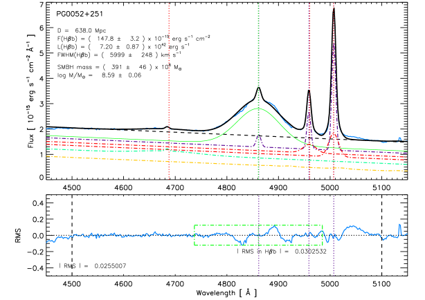
Figure 1: (Top panel) Fit to the emission line profiles of PG 0052+251 observed around the H$\beta$ region. The blue line is the observed spectrum of the quasar, while the black line is the best fit to the data. The black dashed line is the fit to the continuum. Dotted magenta lines indicate the center of the narrow-components for H$\beta$ and [O iii] $\lambda\lambda$4959, 5007. Dotted red lines indicate the center of all the broad components but H$\beta$. The center of the broad H$\beta$ line is plotted by a green dotted line. The continuous green line shows the broad H$\beta$ gaussian. The dotted-dashed magenta line represents the narrow-component spectrum. The dotted-dashed red lines correspond to the broad [O iii] lines. The dotted-dashed green line represents the broad and narrow He ii $\lambda$4686 lines. The dotted-dashed yellow line shows the template Fe ii spectrum (Véron-Cetty, Joly & Véron, 2004) scaled for this object considering the 4500-5100 Å range. Some derived properties of the fit are shown in the top left corner. (Bottom panel) The blue line represents the $rms$ of our fit. The fit has been done within the region between the vertical dashed lines. The average value of the $rms$ is shown in the bottom left corner. The green dashed box indicates the region used to estimate the $rms$ of the broad H$\beta$ component; its average value is also shown. Dotted magenta lines indicate the center of the narrow-components for H$\beta$ and [O iii] $\lambda\lambda$4959, 5007.

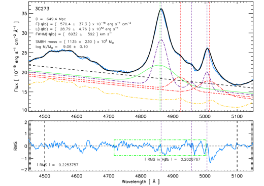
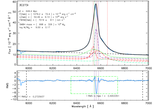
Figure 2: Fit to the emission line profiles of 3C 273 around the H$\beta$ region (top) and the H$\alpha$ region (bottom). The lines are the same described in Fig. 1, following a similar description for the H$\alpha$ fit (the blue line is the observed spectrum, the black line is our best fit, dotted red lines are the center of the broad components but H$\alpha$, which is plotted by a green dotted line; the continuous green line is the broad H$\alpha$ Gaussian, the dotted-dashed magenta line is the narrow H$\alpha$ line; the dotted-dashed red lines are the broad [N ii] lines; and the dotted-dashed green line is a broad He i $\lambda$6678 line).

Table 2: Details of the flux contributions of the He ii, Fe ii and broad H$\beta$  lines to the fits in the 4500-5100 Å  region.

Object	Fe ii	He ii lines			% Fe ii			% He ii			% H$\beta$ broad
		Broad	Narrow		All	broad H$\beta$		All	broad H$\beta$		All	broad H$\beta$
PG 0052+251	VERY FAINTa	VERY FAINT	YES		1.2	0.9		6.9	1.8		56.4	81.0
PHL 909	FAINT	VERY FAINT	YES		7.9	2.6		4.3	0.7		51.4	64.2
PKS 0736+017	YES	YES	YES		17.0	5.7		15.0	2.7		40.5	77.3
3C 273	YES	NO	NO		34.5	5.6		0.0	0.0		20.4	34.1
PKS 1302-102	YES	NO	NO		37.4	4.3		0.0	0.0		38.7	82.2
PG 1309+355	YES	NO	YES		29.2	2.8		0.4	0.0		42.6	69.9
PG 1444+407	YES	NO	NO		54.1	7.7		0.0	0.0		27.9	66.1
PKS 2135-147	VERY FAINTa	VERY FAINT	YES		4.0	0.8		4.2	1.7		43.6	46.3
4C 31.63	YES	NO	NO		38.0	5.8		0.0	0.0		43.9	84.5
PKS 2349-014	FAINT	NO	VERY FAINT		8.2	1.7		0.3	0.0		46.8	75.2

The procedure we followed for performing the fitting in the H$\beta$ region was the following:

1. First, we fit the continuum and broad and narrow components around the He ii $\lambda$4686 emission line (if any).

2. Then, we use the template provided by Véron-Cetty, Joly & Véron (2004) to scale the Fe ii template spectrum only considering the lines in the range 4500-5100 Å by minimizing the fit residuals. However, as I Zw 1 is a narrow line emission galaxy type Seyfert 1, we use the broad Fe ii lines observed in the 4500-4700 Å range for providing a broadening to the Fe ii template spectrum. In any case the contribution of the Fe ii lines in the broad H$\beta$ range is small, typically between 1–6% of the total flux of the derived broad H$\beta$ flux (see Table 2).

3. Then we fit the spectral profile between H$\beta$ and [O iii] using three broad components: the broad H$\beta$ and the broad [O iii] lines. All these components must have sigma $>10$ Å to assure that we are not fitting any narrow line. The scale factor for the Fe ii template spectrum is also included in the minimization of the fit residuals.

4. After that, we add the three narrow emission lines corresponding to the nebular H$\beta$ and [O iii] emission. We forced sigma to be the same in the three lines. As the integrated flux of the [O iii] emission lines is fixed by theory (Osterbrock & Ferland, 2006), we also forced that $F$[O iii] $\lambda$4959 = 0.3467$\times F$[O iii] $\lambda$5007. We then search for those three narrow Gaussians that minimized the residuals.

5. If the narrow H$\beta$ emission seems to be broader than the [O iii] lines, we then fit only this line to get a better solution.

6. We now search for the best combination of narrow+broad Gaussians that fits the [O iii] lines, again forcing the same sigma in both narrow lines and $F$[O iii] $\lambda$4959 = 0.3467$\times F$[O iii] $\lambda$5007 in the narrow lines.

7. Finally, we slightly change the parameters of all Gaussians and search for the combination that minimizes the residuals but keeping all assumptions considered before (e.g., same sigma for narrow lines). This would be our best fit.

We note that, although it is not usually considered (e.g. Mezcua et al., 2011; Fogarty et al., 2012; Ho et al., 2014; Wild et al., 2014; Sánchez et al., 2015), the flux of the broad [O iii] lines could be also fixed following the theory (Osterbrock & Ferland, 2006). However we have considered this assumption for the most challenging case, 3C 273 and note that this assumption leads to a slightly worse fit and it does not materially change the results for the derived values (FWHM, flux, and SMBH mass).

The results of the Gaussians which are providing the best fits are listed in Table 3, while the plots showing these fits and their $rms$ are compiled in Figures 1, 2, and 10 to 15. We note that some of the residuals obtained follow from some small asymmetry of the broad H$\beta$ line or the broad [O iii] $\lambda$5007 line (broad asymmetric wings). These asymmetric features can be fitted using Gauss-Hermite polynomials (e.g, see Park et al., 2012), however their contribution is rather small (few %), so we just include this discrepancy in our final error budget.

We follow a similar procedure for fitting the H$\alpha$ region. In this case, we force $F$[N ii] $\lambda$6548 = 0.3402$\times F$[N ii] $\lambda$6583 for the narrow emission line components. The spectra resolution of some of the spectra obtained around the H$\alpha$ region is low enough to reduce the accuracy of the fitting (particularly in 4C 31.63), but this uncertainty is included in the error budget of the broad H$\alpha$ line. In any case, as we will discuss below, the H$\alpha$-based SMBH masses agree very well with the H$\beta$-based SMBH masses in all objects (differences smaller than 0.06 dex).

Table 3: Results of the best fits to the emission line profiles of our quasar spectra. For each emission line we provide the results for both the narrow (n) and the broad (b) components. We provide the $\sigma$, central wavelength, $c$, and peak, $p$, of a Gaussian fit, $G=p\times\exp\big{[}{-0.5\times(\frac{\lambda-c}{\sigma})^{2}}\big{]}$. We express $p$ in units of 10^-16 erg s^-1 cm^-2, $\sigma$ and $c$ in units of Å. For some few objects we added an extra broad component (e) in H$\beta$ or H$\alpha$, which provides a most robust fit to the data.

Quasar	Comp.	He ii $\lambda$4686				H$\beta$				[O iii] $\lambda$4959				[O iii] $\lambda$5007
		$\sigma$	$c$	$p$		$\sigma$	$c$	$p$		$\sigma$	$c$	$p$		$\sigma$	$c$	$p$
PG0052+251	n	3.69	4684.1	0.836		4.30	4861.4	4.86		3.83	4958.7	14.8		3.83	5006.8	42.8
	b	56.1	4687.7	1.22		41.3	4860.8	14.3		12.2	4960.3	3.37		9.54	5006.5	9.25
PHL909	n	5.78	4687.9	0.482		4.90	4861.0	0.842		4.90	4958.1	3.32		4.90	5006.7	9.58
	b	$\cdots$	$\cdots$	$\cdots$		47.0	4862.6	6.10		21.8	4944.1	2.52		28.1	4989.6	2.86
PKS0736+017	n	5.48	4687.7	0.276		9.15	4863.3	1.05		4.90	4958.9	0.779		4.90	5006.8	2.49
	b	$\cdots$	$\cdots$	$\cdots$		21.8	4866.9	3.81		23.5	4939.2	0.625		36.4	5029.4	0.442
3C273	n	$\cdots$	$\cdots$	$\cdots$		20.2	4864.0	116.6		10.8	4958.9	15.7		10.8	5006.8	45.4
	b	$\cdots$	$\cdots$	$\cdots$		47.7	4860.4	47.7		24.7	4924.0	32.3		33.3	5014.4	34.2
PKS1302-102	n	$\cdots$	$\cdots$	$\cdots$		5.71	4861.6	1.74		5.03	4958.0	2.18		5.03	5006.1	5.41
	b	$\cdots$	$\cdots$	$\cdots$		29.3	4867.9	5.59		13.3	4940.6	1.19		14.6	5003.7	2.52
PG1309+355	n	10.5	4686.7	3.48		4.01	4861.6	18.9		4.01	4958.7	23.1		4.01	5006.7	66.6
	b	$\cdots$	$\cdots$	$\cdots$		43.9	4870.7	40.0		14.6	4954.3	15.5		12.3	5002.4	39.8
PG1444+407	n	$\cdots$	$\cdots$	$\cdots$		12.4	4863.3	8.53		5.14	4958.9	0.771		5.14	5004.0	3.70
	b	$\cdots$	$\cdots$	$\cdots$		29.4	4867.5	12.1		15.9	4941.2	2.56		28.5	5016.6	2.07
PKS2135-147	n	5.04	4686.0	2.26		4.31	4861.8	7.53		4.03	4959.1	31.1		4.03	5006.8	89.7
	b	125.7	4691.4	0.810		58.2	4867.6	10.0		13.6	4961.0	2.33		12.8	5011.1	7.36
4C31.63	n	$\cdots$	$\cdots$	$\cdots$		6.03	4870.7	1.73		5.28	4960.1	2.52		5.28	5006.2	7.85
	b	$\cdots$	$\cdots$	$\cdots$		26.2	4879.0	21.3		13.4	4946.8	4.13		39.3	5018.0	2.82
PKS2349-014	n	4.79	4686.8	0.168		6.09	4863.1	2.01		4.40	4959.0	4.55		4.40	5006.8	13.1
	b	$\cdots$	$\cdots$	$\cdots$		41.66	4862.6	5.13		16.1	4956.1	0.990		16.9	5004.7	2.52
Object	Comp.	[N ii] $\lambda$6548				H$\alpha$				[N ii] $\lambda$6583				He i $\lambda$6678
		$\sigma$	$c$	$p$		$\sigma$	$c$	$p$		$\sigma$	$c$	$p$		$\sigma$	$c$	$p$
3C273	n	2.73	6548.0	5.02		13.0	6562.8	265.1		2.73	6583.4	14.8		$\cdots$	$\cdots$	$\cdots$
	b	16.2	6538.0	113.0		65.1	6547.3	66.1		49.6	6573.0	83.9		62.1	6656.9	26.2
PKS1302-102	n	5.69	6547.2	0.841		5.69	6563.9	6.55		5.69	6584.2	2.43		$\cdots$	$\cdots$	$\cdots$
	b	6.37	6548.6	3.63		39.9	6568.9	11.2		9.38	6577.2	1.71		14.8	6679.1	1.77
PKS2135-147	n	5.72	6547.3	2.70		5.72	6562.1	25.4		5.72	6582.7	7.78		$\cdots$	$\cdots$	$\cdots$
	b	37.6	6467.0	9.50		73.2	6575.7	24.7		46.3	6578.8	10.6		9.51a	6723.3a	2.93a
4C31.63	n	17.42	6525.5	1.01		17.4	6560.6	3.32		17.4	6574.9	2.97		$\cdots$	$\cdots$	$\cdots$
	b	13.22	6546.4	10.6		39.8	6567.5	27.5		19.3	6570.6	15.2		$\cdots$	$\cdots$	$\cdots$
PKS2349-014	n	6.96	6548.1	3.20		6.96	6562.9	11.2		6.96	6582.5	9.39		4.08b	6300.6b	0.881b
	b	16.6	6537.7	8.85		68.0	6583.6	5.03		25.4	6591.3	7.45		11.8a	6723.0a	1.50a

Table 4: Results of the analysis of the emission line profiles of our target quasars. The second column provides the best $rms$ obtained in the fit. The third column indicates if the fit has been performed to the H$\beta$ or H$\alpha$ region. The fourth and fifth columns compile the luminosity and FWHM of the broad H$\beta$ or H$\alpha$ emission line. Columns sixth and seventh give the mass of the SMBH derived using our data following Eqs. 3.2 and 3.2. Last column provides the stellar velocity dispersion, $\sigma_{\star}$, for the analyzed galaxies, which was obtained by Wolf & Sheinis (2008).

		Broad Emission Line
Quasar	$rms$	Line	$L$	FWHM	$M_{\rm SMBH}$	$\log(M_{\rm SMBH}/M_{\odot}$)	log ($\sigma_{\star}$)
	[erg s-1 cm-2 Å-1]		[1042 erg s-1]	[km s-1]	[106 $M_{\odot}$]		[km s-1]
PG0052+251	0.025501	H$\beta$	7.20 $\pm$ 0.87	5999 $\pm$ 248	391 $\pm$ 46	8.59 $\pm$ 0.06	2.45 $\pm$ 0.08
PHL909	0.017113	H$\beta$	4.30 $\pm$ 0.58	6830 $\pm$ 371	380 $\pm$ 52	8.58 $\pm$ 0.06	2.22 $\pm$ 0.03
PKS0736+017	0.008748	H$\beta$	1.49 $\pm$ 0.20	3157 $\pm$ 160	44 $\pm$ 5	7.65 $\pm$ 0.06	2.53 $\pm$ 0.10
3C273	0.225376	H$\beta$	28.8 $\pm$ 4.8	6932 $\pm$ 592	1135 $\pm$ 230	9.06 $\pm$ 0.10	2.52 $\pm$ 0.07
	0.272594	H$\alpha$	54.5 $\pm$ 9.1	7019 $\pm$ 611	998 $\pm$ 326	9.00 $\pm$ 0.17	”
PKS1302-102	0.020744	H$\beta$	6.07 $\pm$ 0.82	4242 $\pm$ 234	177 $\pm$ 25	8.25 $\pm$ 0.07	2.59 $\pm$ 0.08
	0.048395	H$\alpha$	16.6 $\pm$ 2.1	4293 $\pm$ 202	188 $\pm$ 47	8.28 $\pm$ 0.13	”
PG1309+355	0.127747	H$\beta$	29.51 $\pm$ 4.26	6370 $\pm$ 410	972 $\pm$ 163	8.99 $\pm$ 0.08	2.42 $\pm$ 0.05
PG1444+407	0.034493	H$\beta$	12.3 $\pm$ 1.8	4261 $\pm$ 270	265 $\pm$ 42	8.42 $\pm$ 0.08	2.50 $\pm$ 0.03
PKS2135-147	0.036036	H$\beta$	11.7 $\pm$ 1.8	8440 $\pm$ 624	1018 $\pm$ 181	9.01 $\pm$ 0.08	2.49 $\pm$ 0.14
	0.068690	H$\alpha$	36.4 $\pm$ 4.3	7862 $\pm$ 309	1010 $\pm$ 274	9.00 $\pm$ 0.14	”
4C31.63	0.040863	H$\beta$	29.24 $\pm$ 3.57	3795 $\pm$ 160	343 $\pm$ 45	8.54 $\pm$ 0.06	2.51 $\pm$ 0.05
	0.039150	H$\alpha$	57.2 $\pm$ 6.5	4275 $\pm$ 145	369 $\pm$ 103	8.57 $\pm$ 0.14	”
PKS2349-014	0.013422	H$\beta$	3.27 $\pm$ 0.43	6048 $\pm$ 306	255 $\pm$ 33	8.41 $\pm$ 0.06	2.48 $\pm$ 0.08
	0.026210	H$\alpha$	5.24 $\pm$ 0.90	7295 $\pm$ 666	298 $\pm$ 81	8.47 $\pm$ 0.14	”

Finally, we applied Eqs. 3.2 and 3.2 to derive the SMBH masses using the results provided for the best fit to the broad H$\beta$ and H$\alpha$ lines, respectively. The luminosities of the broad H$\beta$ and H$\alpha$ lines were derived just applying the $L=4\pi D^{2}F$ relation. The distance to the quasar, $D$, was determined from the radial velocity of the narrow [O iii] $\lambda$5007 emission line, which was also provided by our fit. Both the redshift $z=v_{rad}/c$ and the distance to our objects (estimated assuming a flat cosmology with $H_{0}$=70 km s^-1 Mpc^-1, $\Omega_{M}$ = 0.3, and $\Omega_{\Lambda}$ = 0.7) are compiled in Table 1. The FWHM was computed using the standard definition for a Gaussian, FWHM = 2.355$\times\sigma$. The results for the luminosity and FWHM of the broad H$\beta$ and/or H$\alpha$ lines of each object are listed in Table 4, which includes the $rms$ obtained in our best fit for each case.

Uncertainties were estimated from the $rms$ of the fit, which provides an error to the derived values for the flux and the $\sigma$ of the Gaussians. For estimating the uncertainty in luminosity we also assumed a 5% error in the absolute flux calibration of our spectra. We propagate these errors through the equations to derive the uncertainties of the SMBH masses, taking into account the uncertainties included in Eqs. 3.2 and 3.2. The H$\alpha$-based SMBH masses have much higher uncertainties than the H$\beta$-based SMBH masses. In any case, we should keep in mind some caveats, uncertainties, and biases of SMBH masses derived using the virial method (see Sect. 3 in Shen, 2013, for a review). For example, as described in the introduction, the actual value of the parameter $f$ introduced in Eq. 2 may vary within a factor of 2–3 depending on the geometry of the BLR. Some other uncertainties are introduced by assuming an unique line profile to infer the underlying BLR velocity structure or considering a single BLR size. The actual effects of the host starlight and the dust reddening (particularly in the blue and UV regimes) are also unknown in many cases, as well as the orientation, isotropy, radiation pressure, and velocity structure of the BLR. Finally, SMBH masses estimated using the virial method may be also affected by the AGN variability.

Table 5: Super-massive black hole mass estimations, in the form of $\log(M_{\rm SMBH}/M_{\odot}$), for the quasars studied in this work (TW) and their estimations found in the literature using different techniques. Forth column compiles the average value of the SMBH mass derived here using the fits to both H$\beta$ and H$\alpha$ broad emission lines. Table includes the derived $f_{5100}$ fluxes (second column and in units of 10${}^{-15}\,$erg s^-1 cm^-2 Å^-1) and the SMBH mass estimations using this value and FWHM_Hβ (third column).

		TW			Reverberation Mapping Techniques
Quasar	$f_{5100}$	$L_{5100}$	Fits		P04	K08	B09	S03	K08	G11
PG 0052+251	1.50 $\pm$ 0.03	8.59 $\pm$ 0.06	8.59 $\pm$ 0.06		8.56 $\pm$ 0.08	8.31 $\pm$ 0.10	8.57 $\pm$ 0.08	$\cdots$	$\cdots$	8.48 $\pm$ 0.26
PHL 909	1.224 $\pm$ 0.014	8.68 $\pm$ 0.06	8.58 $\pm$ 0.06		$\cdots$	$\cdots$	$\cdots$	$\cdots$	9.12 $\pm$ 0.20	$\cdots$
PKS 0736+017	0.430 $\pm$ 0.006	7.77 $\pm$ 0.06	7.65 $\pm$ 0.06		$\cdots$	$\cdots$	$\cdots$	$\cdots$	8.08 $\pm$ 0.20	$\cdots$
3C 273	11.1 $\pm$ 0.4	9.22 $\pm$ 0.09	9.04 $\pm$ 0.08		8.95 $\pm$ 0.08	8.69 $\pm$ 0.08	8.95 $\pm$ 0.09	8.88	$\cdots$	$\cdots$
PKS1302-102	1.30 $\pm$ 0.02	8.52 $\pm$ 0.07	8.26 $\pm$ 0.06		$\cdots$	$\cdots$	$\cdots$	$\cdots$	8.58 $\pm$ 0.30	$\cdots$
PG 1309+355	8.37 $\pm$ 0.05	9.58 $\pm$ 0.08	8.99 $\pm$ 0.09		$\cdots$	$\cdots$	$\cdots$	8.16	8.38 $\pm$ 0.30	$\cdots$
PG 1444+407	1.58 $\pm$ 0.03	10.11 $\pm$ 0.10	8.42 $\pm$ 0.08		$\cdots$	$\cdots$	$\cdots$	$\cdots$	8.21 $\pm$ 0.20	$\cdots$
PKS 2135-147	1.486 $\pm$ 0.018	9.03 $\pm$ 0.07	9.01 $\pm$ 0.07		$\cdots$	$\cdots$	$\cdots$	$\cdots$	8.96 $\pm$ 0.20	$\cdots$
4C 31.63	1.75 $\pm$ 0.02	8.56 $\pm$ 0.06	8.55 $\pm$ 0.05		$\cdots$	$\cdots$	$\cdots$	$\cdots$	8.43 $\pm$ 0.30	$\cdots$
PKS 2349-014	0.620 $\pm$ 0.014	8.68 $\pm$ 0.06	8.43 $\pm$ 0.06		$\cdots$	$\cdots$	$\cdots$	$\cdots$	8.55 $\pm$ 0.20	$\cdots$

References. — (P04) Peterson et al. (2004) using reverberation mapping techniques; (K08) Kim et al. (2008) using the reverberation mapping method; (B09) Bentz et al. (2009b) using reverberation mapping techniques; (S03) Shields et al. (2003); (K08) Kim et al. (2008) using the virial method based on the single epoch spectrum; (G11) Gliozzi et al. (2011) using X-ray data.

For completeness, we also estimated the SMBH masses using the continuum luminosity at rest frame wavelength 5100 Å, $\lambda L_{5100}$, and the FWHM of the broad H$\beta$ emission line derived in our fit, via the virial formula provided by Greene & Ho (2005), see Eq. 3.2. Table 3.2 compiles both the $f_{5100}$ measured in our spectra and the SMBH masses using the derived continuum luminosity. The uncertainty of the $f_{5100}$ flux has been estimated using the $rms$ of the continuum over the $\lambda\lambda$5075-5125 range and does not include the error in the absolute flux calibration. Errors listed in the mass estimations following this method include the uncertainties in both $L_{5100}$ and FWHM_Hβ measurements as well as the uncertainties shown in Eq. 3.2 and the error in the absolute flux calibration.

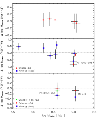
Figure 3: (Top) Comparison of the $M_{SMBH}$ derived here using the H$\alpha$ and H$\beta$ profile fitting. (Middle) Comparison of our $M_{SMBH}$ estimations with the values provided by Shields et al. (2003)–red diamonds– and Kim et al. (2008) –blue boxes–, in both cases derived following the virial method based on the single epoch spectrum. (Bottom) Comparison of our $M_{SMBH}$ estimations with the values provided by Peterson et al. (2004) –red diamonds– and Kim et al. (2008) –blue boxes–, in both cases using reverberation mapping techniques. The value of the $M_{SMBH}$ obtained by Gliozzi et al. (2011) for PG 0052+251 using X ray data is also plotted in this panel –green circle–.

4 Discussion

4.1 Mass comparison

We first compared our derived $M_{SMBH}$ values using the fitting to the H$\alpha$ and H$\beta$ emission line profiles. Top panel of Fig. 3 plots the difference of the logarithm of the masses found using H$\alpha$ and H$\beta$ profile fitting ($y$-axis) versus the mass obtained from the H$\beta$ profile fitting ($x$-axis) for the five quasars we have H$\alpha$ data. As this panel clearly shows, the H$\alpha$-based SMBH masses agree very well with those values derived from the analysis of the H$\beta$ region. The H$\alpha$ spectra typically have lower spectral resolution than the H$\beta$ spectra, and hence higher uncertainties, thus in these five cases we use an uncertainty-weighted average of both results to minimize the error of our SMBH mass estimations, which we compile in Table 3.2. The fact that both the H$\alpha$-based and the H$\beta$-based SMBH mass estimations agree well in all cases reinforces the strength of the technique used here to estimate SMBH masses.

Figure 3 also compares our results for the SMBH masses with those values found in the literature. Table 4 compiles the $M_{\rm SMBH}$ masses of our QSO sample found by other authors following different techniques. We note that we checked for a consistent treatment –i.e., similar virial factor used (within 4 - 8%) for computing SMBG masses– when using literature data. Only two of our quasars have an estimation of their SMBH masses using reverberation mapping techniques: 3C 273 and PG 0052+251 (Kaspi et al., 2000; Peterson et al., 2004; Kim et al., 2008; Bentz et al., 2009b). Following Table 3.2 and the bottom panel of Fig. 3, we see that our results agree well within the errors for PG 0052+251: we derived $\log(M_{\rm SMBH}/M_{\odot}$) = 8.60$\pm$0.06, while Peterson et al. (2004) and Bentz et al. (2009b) estimated SMBH masses of 8.56$\pm$0.08 and 8.57$\pm$0.08, respectively. Kim et al. (2008) derived a somewhat lower mass for the SMBH in this object, 8.31$\pm$0.10. Our result for 3C 273 also agrees within the errors with those values reported in the literature using reverberation mapping techniques: we derived $\log(M_{\rm SMBH}/M_{\odot}$) = 9.04$\pm$0.08 consistently using both the fitting to the H$\alpha$ and H$\beta$ regions, while Peterson et al. (2004) and Bentz et al. (2009b) estimated 8.95$\pm$0.08 and 8.95$\pm$0.09, respectively, for this object. However, Kim et al. (2008) provides again a lower mass for the SMBH within 3C 273, $\log(M_{\rm SMBH}/M_{\odot}$) = 8.69$\pm$0.08. Previous studies of the $M_{SMBH}$ of 3C 273 using the virial method based on a single epoch spectrum also provide lower numbers that we do: Shields et al. (2003) found $\log(M_{\rm SMBH}/M_{\odot}$) = 8.88. We rule out a problem with the absolute flux calibration of our spectrum, as our sample considers other objects that were observed the same night and show no issues with flux calibration. We also consider our analysis, particularly the fitting to the emission line profiles (up to 4 narrow and 5 broad components have been considered), has been performed with more detail than in previous work. However, it is possible that the differing flux measurements of 3C 273 are due to true variations in the emission of this quasar (Lloyd, 1984; Hooimeyer et al., 1992; Ghosh et al., 2000; Soldi et al., 2008). Although following the virial hypothesis an increasing (decreasing) of the emission line luminosities will induce a decreasing (increasing) of the rotational velocity of the gas, uncorrelated physical or observational stochastic variations between line width and luminosity (or other effects as described in Sect. 3.2) may also play an important role in determining the SMBH mass of 3C 273.

Middle panel of Fig. 3 compares our SMBH masses with those estimations obtained by Shields et al. (2003) using the $M_{SMBH}$-$\sigma_{*}$ relation based on the [O iii] sigma and Kim et al. (2008) using the virial method based on a single epoch spectrum. We see a fairly good correlation for some objects (PKS 1302-102, PKS 2135-147, 4C 31.63, PKS 2349-014) which agree well within the errors but for other objects (PHL 909, PKS 0736+017, PG 1309+355, PG 1444+407) we see poor agreement, well outside the error bars. The worst case is PG 1309+355, SMBH mass estimate disagrees by more than an order of magnitude, between the two methods. We believe our results for this object and for PHL 909 provides the most robust estimate of the MBH mass, as the $rms$ of our fits are very low in both cases. Furthermore, as shown in the middle panel of Fig. 3 panel, there appears to be a trend in our fits providing lower SMBH masses than previously estimated in the low-mass end, while obtaining higher SMBH masses than previously estimated in the high-mass end.

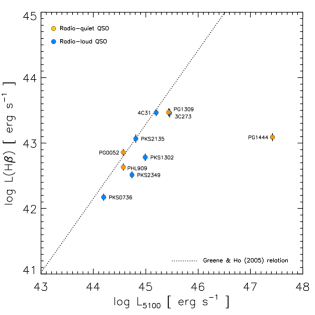
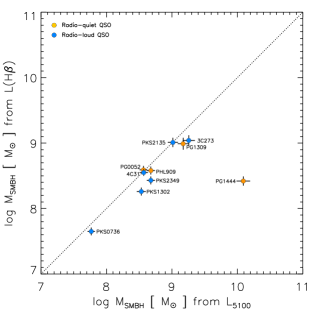
Figure 4: (Left) Comparison between the continuum luminosity at rest frame wavelength 5100 Å, $\lambda L_{5100}$, and the broad H$\beta$ luminosity derived from our fits. The dotted line plots the relationship between both quantities presented by Greene & Ho (2005). (Right) Comparison between the SMBH mass derived using the fits to both the broad H$\alpha$ and H$\beta$ emission lines and that derived from $L_{5100}$ and FWHM_Hβ following Eq. 3.2. The dotted line indicates $y=x$.

The only object in common with the sample analyzed in X rays by Gliozzi et al. (2011) is PG 0052+251 (see bottom panel of Fig. 3). These authors derived $\log(M_{\rm SMBH}/M_{\odot}$) = 8.48$\pm$0.26, which matches within the errors with our result. This also suggests that the value provided by Kim et al. (2008) using reverberation mapping techniques may be slightly underestimated. If this is also the case for 3C 273, it would explain why our $M_{\rm SMBH}$ estimation is higher than that derived by Peterson et al. (2004); Bentz et al. (2009b) and Kim et al. (2008) using reverberation mapping techniques.

Finally, we also study how well the SMBH masses are recovered when using the continuum luminosity at 5100 Å instead of our fits to the emission line profiles. Left panel of Fig. 4 compares the derived $\lambda L_{5100}$ luminosities with the broad H$\beta$ luminosity obtained in our fits. This panel includes the relationship provided by Greene & Ho (2005). Right panel of Fig. 4 compares the SMBH mass computed using $\lambda L_{5100}$ and that obtained from our fits to the broad emission lines. As we see, all but one of our objects have a relatively good agreement between both SMBH estimations, although masses derived using $\lambda L_{5100}$ seem to be systematically overestimated. Indeed, Greene & Ho (2005) already pointed out this result, emphasizing that the effect is serious for relatively luminous, core-dominated sources and, in particular, radio-loud objects. These authors attributed the enhancement of the optical continuum to jet contamination, although they did not rule out that the enhancement is a consequence of changes in the ionizing spectrum or the covering factor of the ionized gas. Nevertheless there is a large difference in masses –almost 3 orders of magnitude– for PG 1444+407, which is a radio-quiet quasar. We consider that the $M_{\rm SMBH}$ estimation derived using our fit to the H$\beta$ emission line profile is much more robust than that obtained from the continuum luminosity. Indeed, if we assume the SMBH mass derived using the $\lambda L_{5100}$ luminosity as the correct one, PG 1444+407 will lie far away from the rest of the radio-quiet quasars in our subsequent analysis of the $M_{\rm SMBH}$-$\sigma_{*}$ relation and $L_{\rm 5\,GHz}$-$\sigma_{*}$ relation.

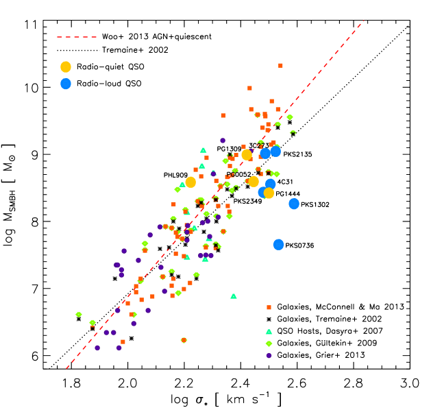
Figure 5: $M_{SMBH}$-$\sigma_{*}$ relation. QSO host galaxies from this work are shown as large circles (radio-loud are blue, radio-quiet are yellow). We also plot the data obtained for quiescent galaxies by Tremaine et al. (2002) –black stars– and by McConnell & Ma (2013) –orange squares–, for radio-quiet PG QSO hosts by Dasyra et al. (2007) –cyan triangles–, for galaxies by Gültekin et al. (2009) –green diamonds–, and for galaxies by Grier et al. (2013) –purple circles–. The black dotted line is the relation derived by Tremaine et al. (2002), and the red dashed line is the recent relation provided by Woo et al. (2013) considering both quiescent galaxies and AGN.

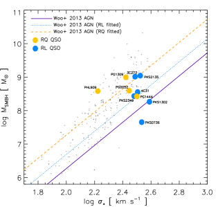
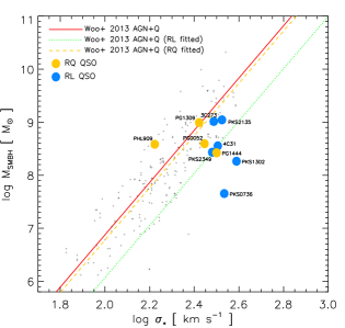
Figure 6: Comparison of our QSO sample datapoints with the new $M_{SMBH}$-$\sigma_{*}$ relations provided by Woo et al. (2013). We consider the cases of only AGN (Left) and AGN + quiescent galaxies (Right) relations. QSO host galaxies from this work are shown as large circles (radio-loud are blue, radio-quiet are yellow). The black crosses represent all the previous data included in Fig. 5. The original $M_{SMBH}$-$\sigma_{*}$ relationships are plotted with a purple (AGN) or red (AGN+quiescent) continuos line. The best fits to the Woo et al. (2013) $M_{SMBH}$-$\sigma_{*}$ relation fixing the slope are plotted with a cyan dotted line (only for AGN and our RL QSO), an orange dashed line (only for AGN and our RQ QSO), a green dotted line (for AGN + quiescent galaxies and our RL QSO), and a dashed yellow line (for AGN + quiescent galaxies and our RQ QSO).

4.2 The $M_{SMBH}$-$\sigma_{*}$ relation

Figure 5 plots the $M_{SMBH}$-$\sigma_{*}$ relation found for our sample. Here we distinguish between RL (blue circles) and RQ (yellow circles) galaxies. Figure 5 includes some data points found in the literature: purple stars plot quiescent galaxies data presented by Tremaine et al. (2002), orange squares indicate galaxy data by McConnell & Ma (2013), cyan triangles are the radio-quiet PG QSO hosts data by Dasyra et al. (2007), the green diamonds represent the galaxy data by Gültekin et al. (2009), and purple circles are galaxy data by Grier et al. (2013). The red dashed line is the recent relation provided by Woo et al. (2013), which considers data of both quiescent galaxies and AGN. The standard $M_{SMBH}$-$\sigma_{*}$ relation derived by Tremaine et al. (2002) is also shown with a dotted black line. As we see, the majority of our quasars seem to agree with these relations, although one object (PKS 0736+017) lies somehow below the Tremaine et al. (2002) relation.

It is also interesting to note the large variations in $M_{SMBH}$-$\sigma_{*}$ within the same $\sigma_{*}$ interval. For example, both PKS 0736+017 and 3C 273 (two radio-loud quasars) have a very similar velocity dispersion, $\log\sigma_{*}\sim 2.52$, while their SMBH masses are differing by almost one and a half orders magnitude, $\log M_{SMBH}=7.65\pm 0.06$ and $9.04\pm 0.08$, respectively.

Some studies (e.g. Grier et al., 2013, and references within) do not find a difference between AGNs and quiescent galaxies on the $M_{SMBH}$-$\sigma_{*}$ relation. However, Woo et al. (2013) investigated the validity of the assumption that quiescent galaxies and active galaxies follow the same relation by updating observational data of both quiescent galaxies and AGN, in the latter case using all available reverberation-mapped AGN. Assuming the standard expression

$$\log\Big{[}\frac{M_{SMBH}}{M_{\odot}}\Big{]}=\alpha+\beta\,\Big{[}\frac{\sigma_{*}}{\rm 200\,km\,s^{-1}}\Big{]},$$ (6)

they derived these relations for the cases of (a) only AGN and (b) AGN + quiescent galaxies. They found that the $M_{SMBH}$-$\sigma_{*}$ of active galaxies (for which $\alpha=7.31\pm 0.15$, $\beta=3.46\pm 0.61$, and the intrinsic scatter is $\epsilon_{0}=0.41\pm 0.05$) appears to be shallower than that of AGN+quiescent galaxies (for which $\alpha=8.36\pm 0.05$, $\beta=4.93\pm 0.28$, and the intrinsic scatter is $\epsilon_{0}=0.43\pm 0.04$). However, Woo et al. (2013) also state that the two relations are actually consistent with one another, as the two different relations are consistent with the same intrinsic $M_{SMBH}$-$\sigma_{*}$ relation due to selection effects.

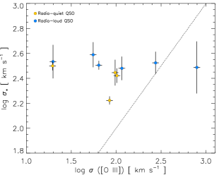
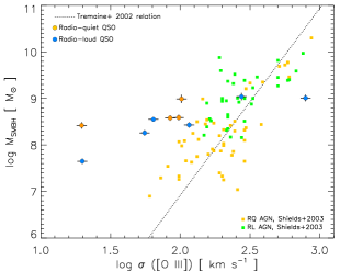
Figure 7: (Left) Comparison between the stellar velocity dispersion, $\sigma_{\star}$, given by Wolf & Sheinis (2008), with the $\sigma$ of the broad [O iii] $\lambda$5007 emission line derived in our fitting. The dotted line represents $x=y$. (Right) The $M_{SMBH}$-$\sigma$ relation using the $\sigma$ of the narrow [O iii] $\lambda$5007. AGN data points by Shields et al. (2003) are plotted with orange squares. In both panels radio-loud QSO are blue circles, radio-quiet QSO are yellow circles.

Table 6: Results of the fittings of our data sample, subdivided in RL and RQ QSO, when compared with the $M_{SMBH}$-$\sigma_{*}$ relationships given by Woo et al. (2013) for AGN and AGN + quiescent galaxies.

	W13 AGN				W13 AGN+Q
	$\alpha$	$\beta$	$\epsilon_{0}$		$\alpha$	$\beta$	$\epsilon_{0}$
W13 original	7.31	3.46	0.657		8.36	4.93	0.870
W13 fitted to RL	7.73	3.46	0.218		7.55	4.93	0.450
W13 original	7.31	3.46	1.144		8.36	4.93	0.603
W13 fitted to RQ	8.31	3.46	0.216		8.26	4.93	0.511

Figure 6 compares our QSO datapoints with the Woo et al. (2013) relationships. The left panel considers their $M_{SMBH}$-$\sigma_{*}$ relation for AGN only (purple solid line), whist the right shows their $M_{SMBH}$-$\sigma_{*}$ relation for AGN and quiescent galaxies (red solid line). We distinguish between radio-loud quasars (RL QSO, blue circles) and radio-quiet quasars (RQ QSO, yellow circles). We now investigate which of these relations fits better to our RL and RQ QSO data when we fixed the slope, $\beta$, and leave the zero point, $\alpha$, free. We search for the $\alpha$ parameter which provides the lowest dispersion between the observational points and these modified relationships for each case, and derive also the intrinsic scatter. Table 6 compiles our results, which are also plotted in Fig, 6. Interestingly, the $M_{SMBH}$-$\sigma_{*}$ relation for AGN and quiescent galaxies provided by Woo et al. (2013) matches well our RQ QSO sample (both lines almost overlap in Fig, 6, as the best fit has $\alpha$=8.26, being the scatter $\epsilon_{0}=0.511$), while the RL QSO sample is in better agreement with the relation for only AGN reported by these authors. In this case, we derive that an $\alpha$=7.73 provides the best match between our observational points and the $M_{SMBH}$-$\sigma_{*}$ relation for only AGN (cyan dotted line).

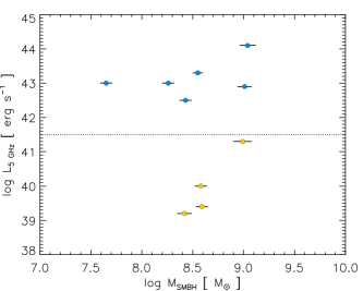
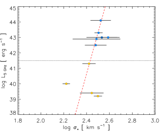
Figure 8: (Left panel) Comparison between the mass derived for the SMBH and the 5 GHz radio-luminosity of the host galaxy, as given by Wold et al. (2010). (Right panel) Comparison between the stellar velocity dispersion of the galaxy hosting a QSO –given by Wolf & Sheinis (2008)– and its 5 GHz radio-luminosity –given by Wold et al. (2010)–. In both panels, radio-loud QSO are blue circles, radio-quiet QSO are yellow circles. We include the limit between RL and RQ quasars as given by $L_{\rm 5\,GHz}\gtrsim 10^{41.5}$ erg s^-1 (Wold et al. 2010). Red dashed line in right panel represents a linear fit to our data

4.3 Comparing stellar velocity dispersions with FWHM of [O iii]

As pointed out in the introduction, the FWHM of the [O iii] $\lambda$5007 emission line has been used by some authors as a surrogate for stellar velocity dispersions (Nelson & Whittle, 1996). In particular, Shields et al. (2003) used $\sigma$([O iii] $\lambda$5007) and not $\sigma_{*}$ to explore the $M_{SMBH}$-$\sigma$ relation, finding a relatively large scatter.

We have compared the stellar velocity dispersions estimated for our sample quasars by Wolf & Sheinis (2008) with the velocity dispersion of the (narrow) [O iii] $\lambda$5007 emission line derived from our fits (see Table 3). Left panel of Fig. 7 compares both velocity dispersions. From this Figure, it is evident that the assumption of using the velocity dispersion of the narrow [O iii] $\lambda$5007 emission line as surrogate for $\sigma_{*}$ is not satisfied. Actually, $\sigma$([O iii] $\lambda$5007) seems to be completely independent of $\sigma_{*}$, particularly for low values.

We further investigate this issue in right panel of Fig. 7, where we plot the $M_{SMBH}$-$\sigma$ relation using $\sigma$([O iii] $\lambda$5007) instead of $\sigma_{*}$. This figure includes the data points compiled by Shields et al. (2003) –which are subdivided in RQ and RL AGN–, as well as the Tremaine et al. (2002) relation. We do not see any correlation at all between the position of our data with the position of the other objects and the relation. Indeed, the Tremaine et al. (2002) relation is valid for only one object. Again, the situation is particularly poor at the low-end of $\sigma$. We therefore conclude that $\sigma$([O iii] $\lambda$5007) should not be used as a surrogate for stellar velocity dispersions for high-mass, high-luminosity quasars.

4.4 Comparing QSO radio-luminosities
with SMBH masses

Nelson & Whittle (1996) reported a rather tight correlation between $\sigma_{*}$ and radio luminosity in Seyfert galaxies, linking directly observable AGN properties to host galaxy properties. Given the subsequent $M_{\rm SMBH}$–$\sigma_{*}$ correlation, one would expect to see a similar correlation between $M_{\rm SMBH}$ and radio luminosity. Such a correlation was reported by Franceschini, Vercellone, & Fabian (1998) for a small sample of 8 nearby early-type galaxies with black hole masses determined from stellar and gas dynamical studies. Later work with more galaxies, both quiescent and active, have shown much larger scatter or no correlation at all (Laor, 2000; Ho, 2002; Snellen et al., 2003; Woo et al., 2005). In fact, a bimodality in radio loudness as a function of $M_{SMBH}$ has been suggested (Laor, 2000).

Left panel of Fig. 8 compares the 5 GHz radio-continuum luminosity, $L_{\rm 5\,GHz}$, of the quasar host galaxy with the derived SMBH masses. The radio data have been extracted from Wold et al. (2010), who estimated $L_{\rm 5\,GHz}$ from previous literature data listed in the NED assuming a spectral index $\alpha=-5$. The limit between RL and RQ quasars –as given by $L_{\rm 5\,GHz}\gtrsim 10^{41.5}$ erg s^-1 following Wold et al. (2010)– is shown in Fig. 8 with a dotted line. Following this figure, we see that RL QSO are found in our entire mass range, including in the low-mass limit –PKS 0736+017, which has $\log(M_{\rm SMBH}/M_{\odot}$) = 7.67$\pm$0.04–. As shown in the left panel of Fig. 8 a correlation between radio loudness and $M_{SMBH}$ is not found in this mass range.

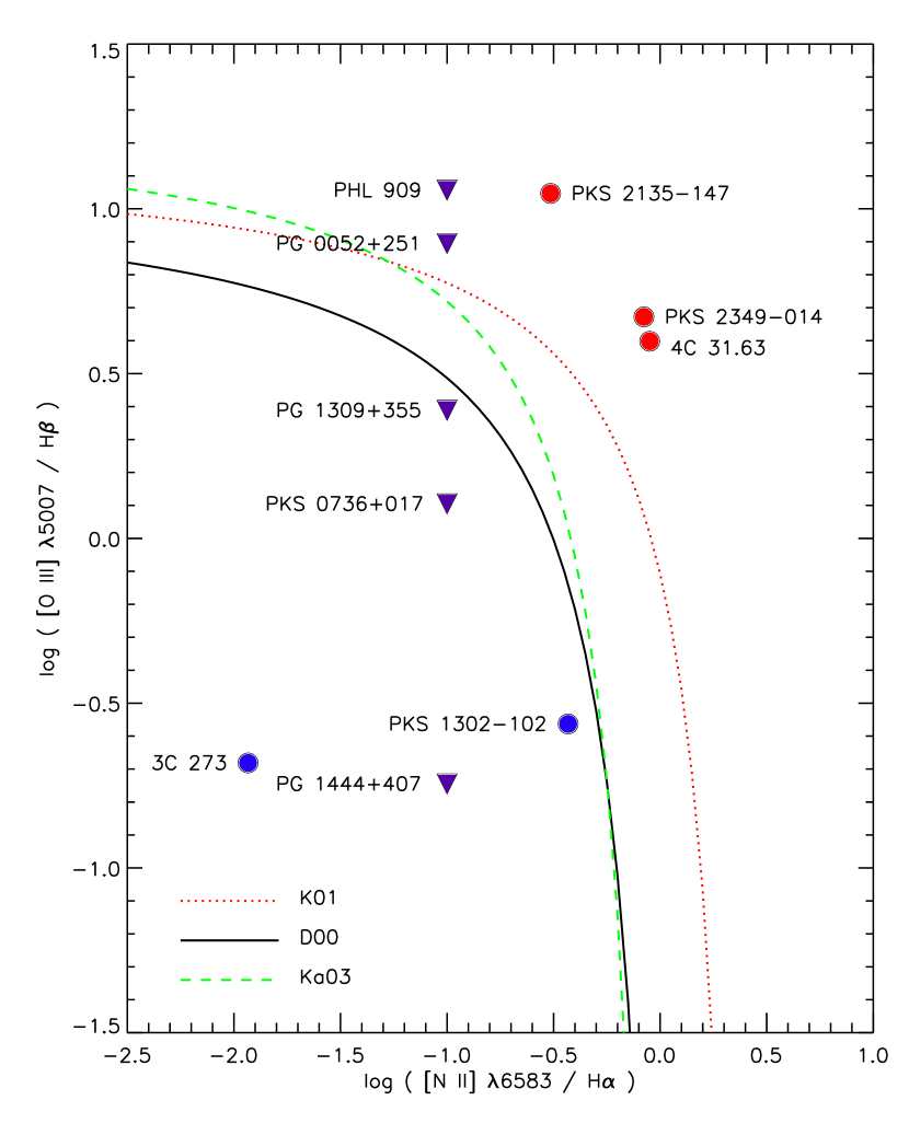
Figure 9: [O iii] $\lambda$5007/H$\beta$ versus [N ii] $\lambda$6583/H$\alpha$ diagnostic diagram for the ionized emission coming from the narrow components of our fits. The loci of the H ii regions as proposed by Dopita et al. (2000), black continuous line (D00), Kewley et al. (2001), red dotted line (K01), and the empirical relation provided by Kauffmann et al. (2003a), dashed green line (Ka03), are also plotted. Circles indicate quasars for which both [O iii] $\lambda$5007/H$\beta$ and [N ii] $\lambda$6583/H$\alpha$ have been measured. In this case, only the narrow components of 3C 273 and PKS 1302-102 (blue circles) are expected to come from photoionization by massive stars, but an important shock contribution is expected in 4C 31.63, PKS 2135-147, and PK 2349-014 (red circles). However, the position of 3C 273 is too far for what expected from H ii regions. Purple triangles indicate the [O iii] $\lambda$5007/H$\beta$ position of objects for which [N ii] $\lambda$6583/H$\alpha$ is unknown.

Conversely, the right panel of of Fig. 8 compares $L_{\rm 5\,GHz}$, with the stellar velocity dispersion of the host galaxy. In this case, we observe a trend that galaxies with larger stellar velocity dispersion have larger 5 GHz radio-continuum luminosities. The red dashed line in this panel represents a linear fit to our data, in the form $\log(L_{\rm 5\,GHz})=A+B\log(\sigma_{*})$, for which we derive $A=-23.3\pm 19.0$, $B=26.6\pm 7.7$. The correlation coefficient is $r$=0.555.

Table 7: Oxygen abundances of the host galaxies using the narrow lines obtained in the fit of our spectra.

Object	[N ii] $\lambda$6583/H$\alpha$	[O iii] $\lambda$5007/H$\beta$	$N2$	$O3N2$	BPT	12 + log (O/H)
						PP04 ($N2$)	PP04 ($O3N2$)	S-B98	Adopted
PG 0052+251	$\cdots$	7.85	$\cdots$	$\cdots$	AGN?	$\cdots$	$\cdots$	$\cdots$	$\cdots$
PHL 909	$\cdots$	11.4	$\cdots$	$\cdots$	AGN?	$\cdots$	$\cdots$	$\cdots$	$\cdots$
PKS 0736+017	$\cdots$	1.27	$\cdots$	$\cdots$	H ii?	$\cdots$	$\cdots$	$\cdots$	$\cdots$
3C 273	0.0116	0.208	-1.936	1.254	H ii?	7.80	8.33	8.34	8.3a
PKS 1302-102	0.370	2.74	-0.870	0.907	H ii	8.65	8.44	8.43	8.55 $\pm$ 0.10
PG 1309+355	$\cdots$	3.53	$\cdots$	$\cdots$	H ii?	$\cdots$	$\cdots$	$\cdots$	8.48?b
PG 1444+407	$\cdots$	0.180	$\cdots$	$\cdots$	H ii?	$\cdots$	$\cdots$	$\cdots$	$\cdots$
PKS 2135-147	0.306	11.1	-0.514	1.560	AGN	8.61	8.23	8.57	8.3 – 8.6
4C 31.63	0.893	3.97	-0.0491	0.648	AGN	8.87	8.52	8.56	8.5 – 8.7
PKS 2349-014	0.839	4.70	-0.0762	0.748	AGN	8.86	8.49	8.56	8.5 – 8.7

4.5 Gas-phase metallicity of the host galaxies

We now use the fitted narrow emission lines to estimate the gas-phase metallicity of the host galaxies. Caution must be taken when attempting to do this, as the physical conditions that are responsible of the ionization of the gas are very different in H ii regions and AGNs. The NLR spectrum is also a function of radiation pressure and, most important, the form of the extreme ultraviolet spectrum. Therefore photoionization models need to be considered to quantitatively derive metallicities in AGN hosts as the typical and very easy-to-apply empirical calibrations involving bright emission-lines used for computing metallicities in H ii regions cannot be applied (e.g., Storchi Bergmann & Pastoriza, 1989; Storchi-Bergmann et al., 1998; Hamann et al., 2002; Groves, Heckman & Kauffmann, 2006; Husemann et al., 2014; Dopita et al., 2014).

We first check that the nature of the ionization of the narrow lines is massive stars (i.e., the narrow lines are produced in star-forming regions) using the [O iii] $\lambda$5007/H$\beta$ versus [N ii] $\lambda$6583/H$\alpha$ diagnostic diagram (Baldwin, Phillips & Terlevich, 1981; Veilleux & Osterbrock, 1987). This diagram is plotted in Fig. 9, and includes the analytic relations given by Dopita et al. (2000) and Kewley et al. (2001), as well as the empirical relation provided by Kauffmann et al. (2003a). The narrow lines derived in 4C 31.63, PKS 2135-147, and PKS 2349-014 (red circles) are still too broad to be produced only for photoionization by massive stars, as these objects do not lie in the loci of the H ii regions in the diagnostic diagram. Hence, other mechanisms, as doppler broadening, outflows, or jet interactions, are playing an important role in the ionization of the lines. Thus, as shown in Fig. 9 we expect that photoionization by massive stars is the main excitation mechanism of the narrow lines in 3C 273 and PKS 1302-102 (blue circles). However, the faintness of the [N ii] $\lambda$6583 line in 3C 273 moves this datapoint too far for what expected for an H ii region, and hence other mechanisms are affecting the ionization of the narrow lines.

Purple triangles in Fig. 9 indicate the [O iii] $\lambda$5007/H$\beta$ position of objects for which [N ii] $\lambda$6583/H$\alpha$ is unknown (i.e., their true $x$-position on this diagram is not known). In the cases of PG 0052+251 and PHL 909, the high [O iii] $\lambda$5007/H$\beta$ value suggests that these objects do not lie in the loci of H ii regions but in the AGN regime (if not, their metallicities should be very low, see Sánchez et al., 2014). On the other hand, the true position of PG 1444+407 –which has the lowest [O iii] $\lambda$5007/H$\beta$ ratio in our sample– in the BPT diagram shown in Fig. 9 may be close to the analytic relations plotted in this figure and therefore consistent with H ii regions. The true position of objects PG 1309+355 and PKS 0736+017 in the BPT diagram may be consistent with H ii regions (in the case $N2\lesssim-0.8$ and $-0.5$, respectively) or LINERs (low-ionization narrow-emission line regions).

As mentioned above, for PKS 1302-102 the ionization of the narrow lines is massive stars. Therefore we can derive its oxygen abundance – in units of 12+log(O/H)– assuming the standard empirical calibrations to derive the metallicity in H ii regions. We use the narrow lines of our fits and apply the standard empirical calibrations obtained by Pettini & Pagel (2004), which consider the $N2=\log$([N ii] $\lambda 6583$/H$\alpha$) and $O3N2=\log${([O iii] $\lambda 5007$/H$\beta$) / ([N ii] $\lambda 6583$/H$\alpha$)} parameters. Table 7 compiles the results of the oxygen abundances obtained following these calibrations and the values of the $N2$ and $O3N2$ parameters when available. However, we note that caution must be taken when using empirical calibrations to derive the oxygen abundance in galaxies (see López-Sánchez et al., 2012, for a recent review about this topic). With this, we derive an oxygen abundance of 8.55$\pm$0.10 for PKS 1302-102. This value is the average oxygen abundance provided by these two empirical calibrations.

The spectrum of PG 1309+355 shows the narrow [O ii] $\lambda$3727 emission line. Assuming that the photoionization of the gas is coming from massive stars (as implied by Fig. 9), we can apply the empirical calibrations given by Pilyugin (2001a, b) –which consider the $R23$ and $P$ parameters, defined as $R_{3}=([\textsc{O\,iii}]\,\lambda 4959+[\textsc{O\,iii}]\,\lambda 5007)/{\rm H\beta}$, $R_{2}=[\textsc{O\,ii}]\,\lambda 3727/{\rm H\beta}$, $R_{23}=R_{3}+R_{2}$, and $P=R_{3}/R_{23}$– to get an estimation of the oxygen abundance of the ionized gas. We consider the Cardelli, Clayton & Mathis (1989) extinction law and assumed a reddening coefficient of $c$(H$\beta$)=0.4 to correct the [O ii] $\lambda$3727 flux for reddening. With this, we derive $f$([O ii] $\lambda$3727)/$f$(H$\beta$) = 0.343, $R23$=46.383, $P$=0.722, and 12+log(O/H)=8.48 for this object.

Storchi-Bergmann et al. (1998) computed the oxygen abundances for an artificial grid of line ratios with the photoionization code CLOUDY (Ferland et al., 1998) using an empirical AGN spectrum for the ionizing source. Storchi-Bergmann et al. (1998) also provided a calibration based on the ([O iii] $\lambda\lambda$4959,5007)/H$\beta$ and ([N ii] $\lambda\lambda$6548,6583)/H$\alpha$ line ratios by fitting a two-dimensional polynomial of second order to their grid of oxygen abundances. We use this calibration to get an estimation of the metallicity in 3C 273, 4C 31.63, PKS 2135-147, and PKS 2349-014. The results are also listed in Table 7. In all four cases we found 12+log(O/H) values between 8.3 and 8.6. As applying the Pettini & Pagel (2004) $N2$ calibration in AGNs will provide higher oxygen abundances than their true value, their results can be considered upper limits to the real metallicity of these objects. Hence, 4C 31.63, PKS 2135-147, and PKS 2349-014 seem to have oxygen abundances between 8.3 and 8.7. For the case of 3C 273, only the Storchi-Bergmann et al. (1998) equation can be used, we provide a tentative value of 12+log(O/H)$\sim$8.3 for its oxygen abundance. Although its real value may be slightly higher, the metallicity of 3C 273 is definitively subsolar.

These are the first attempt of deriving the gas-phase oxygen abundance in these quasars we are aware of. It is challenging to derive the oxygen abundances in active galaxies due to the strong contamination of the broad emission lines created by the AGN activity. However, detailed analyses indicate that most AGN tend to have solar –12+log(O/H)_⊙=8.69, Asplund et al. (2009)– to supersolar metallicities (Storchi Bergmann & Pastoriza, 1989; Storchi-Bergmann et al., 1998; Hamann et al., 2002), reinforcing the hypothesis that AGN are usually found at high metallicities. Recently, Husemann et al. (2014) used the narrow emission lines to estimate the oxygen abundances of 11 low redshift ($z<0.2$) quasar host galaxies, all of them ranging between 8.5 and 9.0 (in the $T_{e}$-based absolute scale). Conversely, only few galaxies hosting AGN are found to have sub-solar metallicities, having in all cases masses lower than 10¹⁰ $M_{\odot}$ (e.g., Groves, Heckman, & Kauffmann, 2006; Barth, Greene, & Ho, 2008; Izotov, Thuan, & Guseva, 2007). In particular, out of a sample of $\sim$23000 Seyfert 2 galaxies, Groves, Heckman & Kauffmann (2006) found only $\sim$40 clear clear candidates for AGN with NLR abundances that are below solar. Low-metallicity AGN seem to be extremely rare (Izotov & Thuan, 2008; Izotov et al., 2010). Hence, it is interesting to note that the oxygen abundances derived for our quasar sample are in the subsolar regime (metallicities between 0.4 Z_⊙ and  Z_⊙). This may suggest that low-$z$, higher luminosity quasars have higher probability of being found in subsolar metallicity hosts than low-luminosity quasars. This is a reasonable argument, as brighter AGNs are expected to consume more gas, suggesting these AGNs are found in host galaxies with large gas reservoirs, and hence lower metallicity as the gas has not yet been primarily processed into stars.

4.6 On the nature of the RL and RQ quasars

Is there a true physical difference between RL and RQ quasars beyond their radio luminosity? Laor (2000) found that virtually all of the RL quasars contain SMBH with masses $M_{\rm SMBH}>10^{9}$$M_{\odot}$, whereas the majority of the RQ quasars host a SMBH with masses $M_{\rm SMBH}<3\times 10^{8}$$M_{\odot}$. Lacy et al. (2001) established that a continuous variation of radio luminosity with BH mass existed and that the radio power also depends on the accretion rate relative to the Eddington limit. Later, McLure & Dunlop (2002) found a similar result, quantifying that the median BH mass of the RL quasars are a factor 2 larger than that of their RQ counterparts. However, Ho (2002) and Jarvis & McLure (2002) found no clear relationship between radio power and black hole mass. McLure & Jarvis (2004) used a sample of more than 6000 quasars from SDSS to find that RL quasars are found to harbour systematically more massive black holes than are the RQ quasars. These authors also reported a strong correlation between radio luminosity and SMBH mass.

RQ quasars seem to be associated with mixed morphologies including spiral galaxies, as they tend to have lower $\sigma_{*}$ than RL quasars (Wolf & Sheinis, 2008). Recently Kimball et al. (2011) used the Expanded Very Large Array (EVLA) to observe at 6 GHz 179 quasars in the redshift range $0.2<z<0.3$, detecting 97% of them. These authors concluded that the radio luminosity function is consistent with the hypothesis that the radio emission in RL quasars is powered primary by AGNs, while the radio emission in RQ quasars is powered primarily by star-formation in their host galaxies (i.e., their host galaxies are spiral galaxies).

Although we consider only the study of 10 objects, our analysis appears to agree with Kimball et al. (2011) conclusions, as it suggests that the $M_{SMBH}$-$\sigma_{*}$ relation of RQ quasars matches well with that found in AGN+quiescent galaxies (i.e., still star-forming galaxies) and that the $M_{SMBH}$-$\sigma_{*}$ relation of RL quasars follows that found only in AGN. Indeed, stellar population synthesis analyses of quasars have shown that the radio-luminosity of RQ quasars is consistent with that found in quiescent star-forming galaxies (Wold et al., 2010). Following our analysis, PG 1309+355, a RQ quasar, also seems to show a relatively important star-formation activity. The importance of the star-formation activity in the quasar host galaxy may be just another consequence of whatever physical phenomenon is responsible for its RL or RQ nature.

As presented in Wolf & Sheinis (2008), we hypothesize that RQ quasars may be formed by a more secular merger scenario than RL quasars, in that many RL quasars show signs of recent or ongoing interactions including major merger events (Zakamska et al., 2006; Villar-Martín et al., 2011, 2012; Bessiere et al., 2012; Villar-Martín et al., 2013). Low surface brightness fine structure indicate of past merger events can easily be missed if too shallow images are used (e.g. Bennert et al., 2008, and references within). However Ramos Almeida et al. (2012) recently found that $\sim$95% of their radio-loud AGN host show interaction signatures, and suggested that radio-loud quasars are also triggered by interactions. In the case or RQ quasars, the merger scenario appears much more rare and may point to RL quasars likely occurring in harassment and minor merger events (whose features can be difficult to detect even in deep images). If this is the case, it is also possible that the major mergers are more likely to lead to binary black holes (Begelman, Blandford & Rees, 1980; Roos, 1981; Khan, Just & Merritt, 2011) as the BH mass scales with galaxy mass while RQ quasars events are characterize by minor mergers in which only a single BH survives due to the mass disparity. The merger of two SMBH seems to be the most plausible scenario to explain the X-shaped morphology observed in some bright radio-galaxies (Merritt & Ekers, 2002; Hodges-Kluck et al., 2010; Gong, Li & Zhang, 2011; Mezcua et al., 2011, 2012). The scenario where the AGN s radio luminosity is fueled by binary BH activity is consistent with our host galaxy observations (RL hosts tend to be more massive than RQ hosts, Wolf & Sheinis, 2008), with the observational result that RL quasars harbour systematically more massive black holes than the RQ quasars (McLure & Dunlop, 2002; McLure & Jarvis, 2004), as well as the observation by Kimball et al. (2011) that show the radio luminosity of the stellar component of the galaxy is a much smaller contribution to the total radio luminosity on RL quasars. These ideas require further exploration.

5 Conclusions

We have analyzed the emission line profiles of a sample of 10 quasars and derive their super-massive black hole masses following the virial method. Our sample consists in 6 radio-loud quasars and 4 radio-quiet quasars. We carefully fit a broad and narrow Gaussian component for each bright emission line in both the H$\beta$ (10 objects) and H$\alpha$ regions (5 objects). Our main conclusions are:

1. We find a very good agreement of the derived SMBH masses, $M_{\rm SMBH}$, using the fitted broad H$\beta$ and H$\alpha$ emission lines. We compare our $M_{\rm SMBH}$ results with those found by previous studies using the reverberation mapping technique, the virial method and X-ray data, as well as those derived using the continuum luminosity at 5100 Å.

2. We study the relationship between the $M_{\rm SMBH}$ of the quasar and the stellar velocity dispersion, $\sigma_{*}$, of the host galaxy. We use the measured $M_{\rm SMBH}$ and $\sigma_{*}$ to investigate the $M_{\rm SMBH}$ – $\sigma_{*}$ relation for both the radio-loud and radio-quiet subsamples. Besides the scatter and the low number of objects in our sample, we find a good agreement between radio-quiet quasars and AGN+quiescent galaxies and between radio-loud quasars and AGN. The intercept in the latter case is 0.5 dex lower than in the first case. Our results support the idea that both the star-formation phenomena in the host galaxy and the RL or RQ nature of the quasar are a consequence of a different merger scenario, possibly being RL quasars triggered by a major merger event and RQ quasars ignited by a minor merger event. Major mergers are more likely to lead to binary black holes, which inter-relationship may drastically enhance the radio activity.

3. Our analysis does not support the hypothesis of using $\sigma$([O iii] $\lambda$5007) as a surrogate for stellar velocity dispersions in high-mass, high-luminosity quasars.

4. We also investigate the relationship between the 5 GHz radio-continuum luminosity, $L_{\rm 5\,GHz}$, of the quasar host galaxy with both $M_{\rm SMBH}$ and $\sigma_{*}$. We do not find any correlation between $L_{\rm 5\,GHz}$ and $M_{\rm SMBH}$, although we observe a trend that galaxies with larger stellar velocity dispersions have larger 5 GHz radio-continuum luminosities.

5. Using the results of our fitting for the narrow emission lines of [O iii] $\lambda$5007 and [N ii] $\lambda$6583 we estimate the gas-phase oxygen abundance of six quasars, being sub-solar in all cases. These are the first attempt of deriving the gas-phase oxygen abundance in these quasars we know of. We suggest that low-$z$, higher luminosity quasars have higher probability of being found in subsolar metallicity hosts than low-luminosity quasars, as the latter have probably processed more gas into stars than high-luminosity quasars.

6 Appendix

Figures 10 to 15 show the fit to the emission line profiles of the rest of our quasar sample, following the same conventions we specified in Figs. 1 and 2.

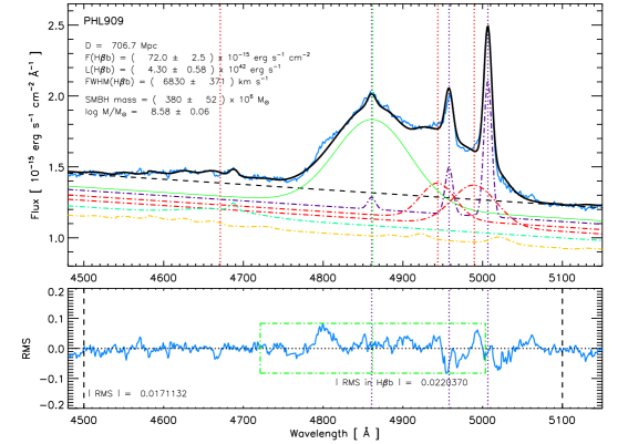
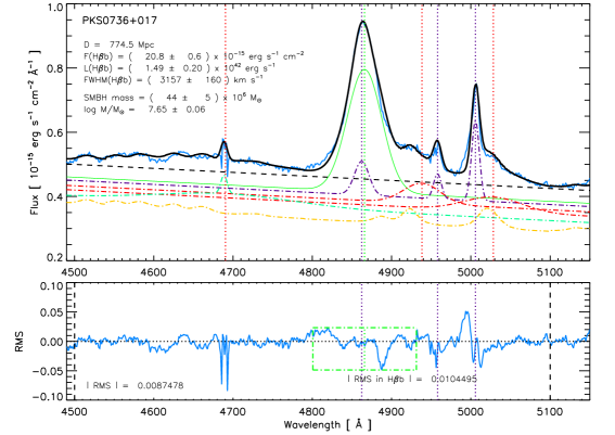
Figure 10: Fit to the emission line profiles of PHL 909 and PKS 0736+017 around the H$\beta$ region. The lines are the same described in Fig. 1.

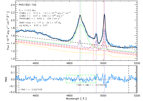
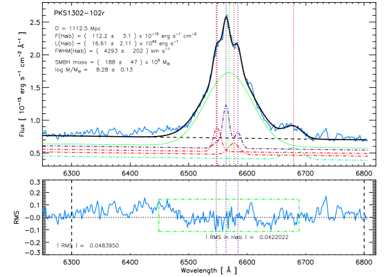
Figure 11: Fit to the emission line profiles of PKS 1302-102 around the H$\beta$ region (top) and the H$\alpha$ region (bottom). The lines are the same described in Fig. 1, following the same procedure for H$\alpha$ as described in Fig. 2.

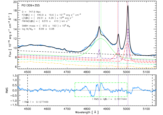
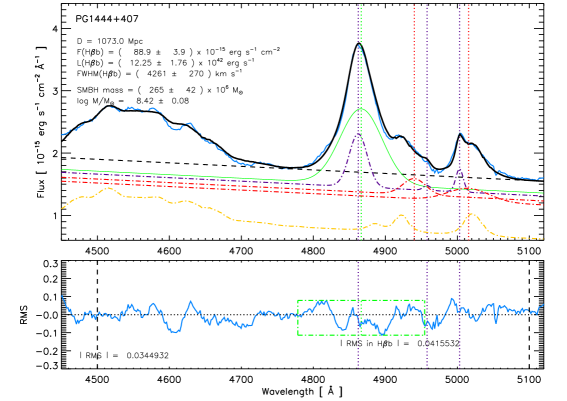
Figure 12: Fit to the emission line profiles of PG 1309+355 and PG 1444+407 around the H$\beta$ region. The lines are the same described in Fig. 1.

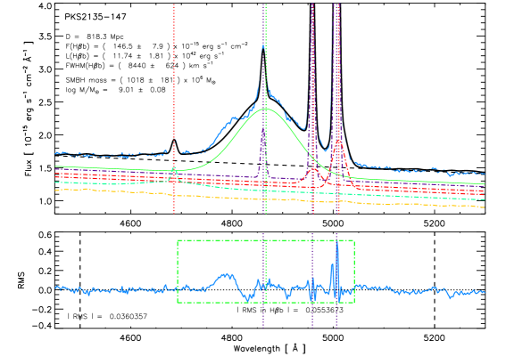
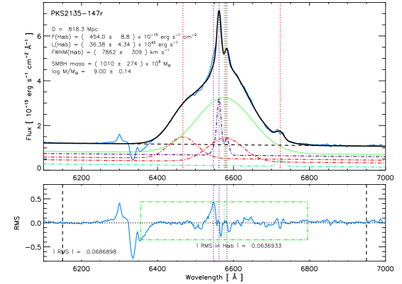
Figure 13: Fit to the emission line profiles of PKS 2135-147 around the H$\beta$ region (top) and the H$\alpha$ region (bottom). The lines are the same described in Fig. 1, following the same procedure for H$\alpha$ as described in Fig. 2. For the H$\alpha$ fit the dotted-dashed green line is a broad [S ii] $\lambda$6717+$\lambda$6731 line.

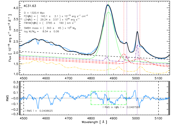
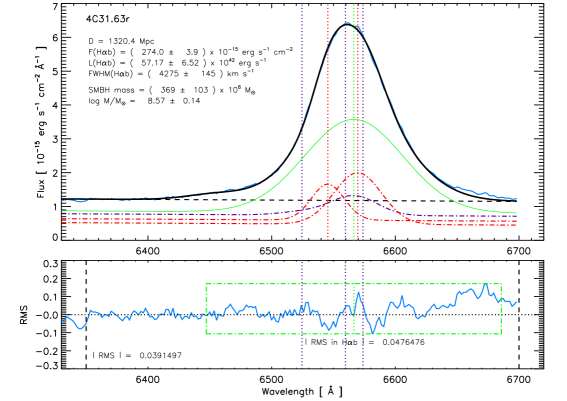
Figure 14: Fit to the emission line profiles of 4C 31.63 around the H$\beta$ region (top) and the H$\alpha$ region (bottom). The lines are the same described in Fig. 1, following the same procedure for H$\alpha$ as described in Fig. 2.

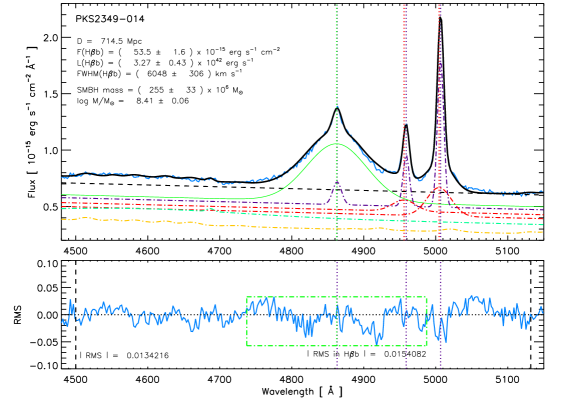
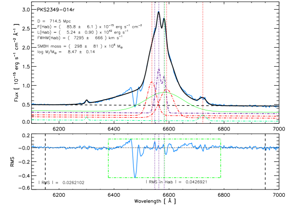
Figure 15: Fit to the emission line profiles of PKS 2349-014 around the H$\beta$ region (top) and the H$\alpha$ region (bottom). The lines are the same described in Fig. 1, following the same procedure for H$\alpha$  as described in Fig. 2. For the H$\alpha$ fit the dotted-dashed green line is a narrow [O i] $\lambda$6730 and a broad [S ii] $\lambda$6717+$\lambda$6731 line.

References

- Asplund et al. (2009) Asplund M., Grevesse N., Sauval A. J., Scott P., 2009, ARA&A, 47, 481
- Assef et al. (2011) Assef R. J. et al., 2011, ApJ, 742, 93
- Bahcall et al. (1997) Bahcall J. N., Kirhakos S., Saxe D. H., Schneider D. P., 1997, ApJ, 479, 642
- Baldry et al. (2004) Baldry I. K., Glazebrook K., Brinkmann J., Ivezić Ž., Lupton R. H., Nichol R. C., Szalay A. S., 2004, ApJ, 600, 681
- Baldwin, Phillips & Terlevich (1981) Baldwin J. A., Phillips M. M., Terlevich R., 1981, PASP, 93, 5
- Barth, Greene & Ho (2008) Barth A. J., Greene J. E., Ho L. C., 2008, AJ, 136, 1179
- Begelman, Blandford & Rees (1980) Begelman M. C., Blandford R. D., Rees M. J., 1980, Nature, 287, 307
- Bell et al. (2004) Bell E. F. et al., 2004, ApJ, 608, 752
- Bennert et al. (2008) Bennert N., Canalizo G., Jungwiert B., Stockton A., Schweizer F., Peng C. Y., Lacy M., 2008, ApJ, 677, 846
- Bentz et al. (2013) Bentz M. C. et al., 2013, ApJ, 767, 149
- Bentz et al. (2010) Bentz M. C. et al., 2010, ApJ, 720, L46
- Bentz et al. (2009a) Bentz M. C., Peterson B. M., Netzer H., Pogge R. W., Vestergaard M., 2009a, ApJ, 697, 160
- Bentz et al. (2009b) Bentz M. C., Peterson B. M., Pogge R. W., Vestergaard M., 2009b, ApJ, 694, L166
- Bentz et al. (2006) Bentz M. C., Peterson B. M., Pogge R. W., Vestergaard M., Onken C. A., 2006, ApJ, 644, 133
- Bernardi et al. (2003) Bernardi M. et al., 2003, AJ, 125, 1882
- Bershady et al. (2004) Bershady M. A., Andersen D. R., Harker J., Ramsey L. W., Verheijen M. A. W., 2004, PASP, 116, 565
- Bershady et al. (2005) Bershady M. A., Andersen D. R., Verheijen M. A. W., Westfall K. B., Crawford S. M., Swaters R. A., 2005, ApJS, 156, 311
- Bessiere et al. (2012) Bessiere P. S., Tadhunter C. N., Ramos Almeida C., Villar Martín M., 2012, MNRAS, 426, 276
- Blandford & McKee (1982) Blandford R. D., McKee C. F., 1982, ApJ, 255, 419
- Boroson & Green (1992) Boroson T. A., Green R. F., 1992, ApJS, 80, 109
- Bryant et al. (2015) Bryant J. J. et al., 2015, MNRAS, 447, 2857
- Cardelli, Clayton & Mathis (1989) Cardelli J. A., Clayton G. C., Mathis J. S., 1989, ApJ, 345, 245
- Cattaneo et al. (2006) Cattaneo A., Dekel A., Devriendt J., Guiderdoni B., Blaizot J., 2006, MNRAS, 370, 1651
- Cid Fernandes et al. (2005) Cid Fernandes R., Mateus A., Sodré L., Stasińska G., Gomes J. M., 2005, MNRAS, 358, 363
- Cimatti et al. (2002) Cimatti A. et al., 2002, A&A, 381, L68
- Croom et al. (2012) Croom S. M. et al., 2012, MNRAS, 421, 872
- Czerny & Nikołajuk (2010) Czerny B., Nikołajuk M., 2010, Mem. Soc. Astron. Italiana, 81, 281
- Dasyra et al. (2007) Dasyra K. M. et al., 2007, ApJ, 657, 102
- Decarli et al. (2008) Decarli R., Labita M., Treves A., Falomo R., 2008, MNRAS, 387, 1237
- Dekel & Birnboim (2006) Dekel A., Birnboim Y., 2006, MNRAS, 368, 2
- Denney et al. (2009a) Denney K. D., Peterson B. M., Dietrich M., Vestergaard M., Bentz M. C., 2009a, ApJ, 692, 246
- Denney et al. (2009b) Denney K. D., Peterson B. M., Dietrich M., Vestergaard M., Bentz M. C., 2009b, ApJ, 692, 246
- Dopita et al. (2000) Dopita M. A., Kewley L. J., Heisler C. A., Sutherland R. S., 2000, ApJ, 542, 224
- Dopita et al. (2014) Dopita M. A. et al., 2014, A&A, 566, A41
- Drory et al. (2001) Drory N., Feulner G., Bender R., Botzler C. S., Hopp U., Maraston C., Mendes de Oliveira C., Snigula J., 2001, MNRAS, 325, 550
- Dunlop et al. (2003) Dunlop J. S., McLure R. J., Kukula M. J., Baum S. A., O’Dea C. P., Hughes D. H., 2003, MNRAS, 340, 1095
- Fabian (1999) Fabian A. C., 1999, MNRAS, 308, L39
- Ferland et al. (1998) Ferland G. J., Korista K. T., Verner D. A., Ferguson J. W., Kingdon J. B., Verner E. M., 1998, PASP, 110, 761
- Ferrarese & Merritt (2000) Ferrarese L., Merritt D., 2000, ApJ, 539, L9
- Ferrarese et al. (2001) Ferrarese L., Pogge R. W., Peterson B. M., Merritt D., Wandel A., Joseph C. L., 2001, ApJ, 555, L79
- Fogarty et al. (2012) Fogarty L. M. R. et al., 2012, ApJ, 761, 169
- Franceschini, Vercellone & Fabian (1998) Franceschini A., Vercellone S., Fabian A. C., 1998, MNRAS, 297, 817
- Fu & Stockton (2009) Fu H., Stockton A., 2009, ApJ, 696, 1693
- Gadotti & Kauffmann (2009) Gadotti D. A., Kauffmann G., 2009, MNRAS, 399, 621
- García-Benito et al. (2015) García-Benito R. et al., 2015, A&A, 576, A135
- García-Lorenzo et al. (2015) García-Lorenzo B. et al., 2015, A&A, 573, A59
- Gebhardt et al. (2000a) Gebhardt K. et al., 2000a, ApJ, 539, L13
- Gebhardt et al. (2003) Gebhardt K. et al., 2003, ApJ, 597, 239
- Gebhardt et al. (2000b) Gebhardt K. et al., 2000b, ApJ, 543, L5
- Ghosh et al. (2000) Ghosh K. K., Ramsey B. D., Sadun A. C., Soundararajaperumal S., 2000, ApJS, 127, 11
- Giavalisco et al. (2004) Giavalisco M. et al., 2004, ApJ, 600, L93
- Gliozzi et al. (2011) Gliozzi M., Titarchuk L., Satyapal S., Price D., Jang I., 2011, ApJ, 735, 16
- Gong, Li & Zhang (2011) Gong B. P., Li Y. P., Zhang H. C., 2011, ApJ, 734, L32
- Graham (2008a) Graham A. W., 2008a, ApJ, 680, 143
- Graham (2008b) Graham A. W., 2008b, PASA, 25, 167
- Graham & Li (2009) Graham A. W., Li I.-h., 2009, ApJ, 698, 812
- Graham et al. (2011) Graham A. W., Onken C. A., Athanassoula E., Combes F., 2011, MNRAS, 412, 2211
- Greene & Ho (2005) Greene J. E., Ho L. C., 2005, ApJ, 630, 122
- Greene, Ho & Barth (2008) Greene J. E., Ho L. C., Barth A. J., 2008, ApJ, 688, 159
- Greene et al. (2010) Greene J. E. et al., 2010, ApJ, 721, 26
- Grier et al. (2013) Grier C. J. et al., 2013, ApJ, 773, 90
- Groves, Heckman & Kauffmann (2006) Groves B. A., Heckman T. M., Kauffmann G., 2006, MNRAS, 371, 1559
- Gültekin et al. (2009) Gültekin K. et al., 2009, ApJ, 698, 198
- Guyon, Sanders & Stockton (2006) Guyon O., Sanders D. B., Stockton A., 2006, ApJS, 166, 89
- Hamann et al. (2002) Hamann F., Korista K. T., Ferland G. J., Warner C., Baldwin J., 2002, ApJ, 564, 592
- Heavens et al. (2004) Heavens A., Panter B., Jimenez R., Dunlop J., 2004, Nature, 428, 625
- Ho et al. (2014) Ho I.-T. et al., 2014, MNRAS, 444, 3894
- Ho (1999) Ho L., 1999, in Astrophysics and Space Science Library, Vol. 234, Observational Evidence for the Black Holes in the Universe, Chakrabarti S. K., ed., p. 157
- Ho (2002) Ho L. C., 2002, ApJ, 564, 120
- Hodges-Kluck et al. (2010) Hodges-Kluck E. J., Reynolds C. S., Miller M. C., Cheung C. C., 2010, ApJ, 717, L37
- Hogg et al. (2003) Hogg D. W. et al., 2003, ApJ, 585, L5
- Holt, Tadhunter & Morganti (2008) Holt J., Tadhunter C. N., Morganti R., 2008, MNRAS, 387, 639
- Hooimeyer et al. (1992) Hooimeyer J. R. A., Miley G. K., de Waard G. J., Schilizzi R. T., 1992, A&A, 261, 9
- Hu et al. (2008) Hu C., Wang J.-M., Ho L. C., Chen Y.-M., Bian W.-H., Xue S.-J., 2008, ApJ, 683, L115
- Husemann et al. (2014) Husemann B., Jahnke K., Sánchez S. F., Wisotzki L., Nugroho D., Kupko D., Schramm M., 2014, MNRAS, 443, 755
- Izotov et al. (2010) Izotov Y. I., Guseva N. G., Fricke K. J., Stasińska G., Henkel C., Papaderos P., 2010, A&A, 517, A90
- Izotov & Thuan (2008) Izotov Y. I., Thuan T. X., 2008, ApJ, 687, 133
- Izotov, Thuan & Guseva (2007) Izotov Y. I., Thuan T. X., Guseva N. G., 2007, ApJ, 671, 1297
- Jarvis & McLure (2002) Jarvis M. J., McLure R. J., 2002, MNRAS, 336, L38
- Jorgensen, Franx & Kjaergaard (1995) Jorgensen I., Franx M., Kjaergaard P., 1995, MNRAS, 276, 1341
- Kang et al. (2013) Kang W.-R., Woo J.-H., Schulze A., Riechers D. A., Kim S. C., Park D., Smolcic V., 2013, ApJ, 767, 26
- Kaspi et al. (2005) Kaspi S., Maoz D., Netzer H., Peterson B. M., Vestergaard M., Jannuzi B. T., 2005, ApJ, 629, 61
- Kaspi et al. (2000) Kaspi S., Smith P. S., Netzer H., Maoz D., Jannuzi B. T., Giveon U., 2000, ApJ, 533, 631
- Kauffmann et al. (2003a) Kauffmann G. et al., 2003a, MNRAS, 346, 1055
- Kauffmann et al. (2003b) Kauffmann G. et al., 2003b, MNRAS, 341, 54
- Kewley et al. (2001) Kewley L. J., Dopita M. A., Sutherland R. S., Heisler C. A., Trevena J., 2001, ApJ, 556, 121
- Khan, Just & Merritt (2011) Khan F. M., Just A., Merritt D., 2011, ApJ, 732, 89
- Kim et al. (2008) Kim M., Ho L. C., Peng C. Y., Barth A. J., Im M., Martini P., Nelson C. H., 2008, ApJ, 687, 767
- Kimball et al. (2011) Kimball A. E., Kellermann K. I., Condon J. J., Ivezić Ž., Perley R. A., 2011, ApJ, 739, L29
- King (2010) King A. R., 2010, MNRAS, 408, L95
- Koo et al. (2005) Koo D. C. et al., 2005, ApJS, 157, 175
- Kormendy, Bender & Cornell (2011) Kormendy J., Bender R., Cornell M. E., 2011, Nature, 469, 374
- Kormendy, Gebhardt & Richstone (2000) Kormendy J., Gebhardt K., Richstone D., 2000, in Bulletin of the American Astronomical Society, Vol. 32, American Astronomical Society Meeting Abstracts #196, p. 702
- Kormendy & Richstone (1995) Kormendy J., Richstone D., 1995, ARA&A, 33, 581
- Krolik (2001) Krolik J. H., 2001, ApJ, 551, 72
- Labbé et al. (2003) Labbé I. et al., 2003, AJ, 125, 1107
- Lacy et al. (2001) Lacy M., Laurent-Muehleisen S. A., Ridgway S. E., Becker R. H., White R. L., 2001, ApJ, 551, L17
- Laor (2000) Laor A., 2000, ApJ, 543, L111
- Liu et al. (2013a) Liu G., Zakamska N. L., Greene J. E., Nesvadba N. P. H., Liu X., 2013a, MNRAS, 430, 2327
- Liu et al. (2013b) Liu G., Zakamska N. L., Greene J. E., Nesvadba N. P. H., Liu X., 2013b, MNRAS, 436, 2576
- Lloyd (1984) Lloyd C., 1984, MNRAS, 209, 697
- López-Sánchez et al. (2012) López-Sánchez Á. R., Dopita M. A., Kewley L. J., Zahid H. J., Nicholls D. C., Scharwächter J., 2012, MNRAS, 426, 2630
- Mathur et al. (2012) Mathur S., Fields D., Peterson B. M., Grupe D., 2012, ApJ, 754, 146
- McCarthy et al. (2004) McCarthy P. J. et al., 2004, ApJ, 614, L9
- McConnell & Ma (2013) McConnell N. J., Ma C.-P., 2013, ApJ, 764, 184
- McConnell et al. (2011) McConnell N. J., Ma C.-P., Gebhardt K., Wright S. A., Murphy J. D., Lauer T. R., Graham J. R., Richstone D. O., 2011, Nature, 480, 215
- McGill et al. (2008) McGill K. L., Woo J.-H., Treu T., Malkan M. A., 2008, ApJ, 673, 703
- McLure & Dunlop (2002) McLure R. J., Dunlop J. S., 2002, MNRAS, 331, 795
- McLure & Jarvis (2002) McLure R. J., Jarvis M. J., 2002, MNRAS, 337, 109
- McLure & Jarvis (2004) McLure R. J., Jarvis M. J., 2004, MNRAS, 353, L45
- Merritt & Ekers (2002) Merritt D., Ekers R. D., 2002, Science, 297, 1310
- Mezcua et al. (2012) Mezcua M., Chavushyan V. H., Lobanov A. P., León-Tavares J., 2012, A&A, 544, A36
- Mezcua et al. (2011) Mezcua M., Lobanov A. P., Chavushyan V. H., León-Tavares J., 2011, A&A, 527, A38
- Miller & Sheinis (2003) Miller J. S., Sheinis A. I., 2003, ApJ, 588, L9
- Nelson et al. (2004) Nelson C. H., Green R. F., Bower G., Gebhardt K., Weistrop D., 2004, ApJ, 615, 652
- Nelson & Whittle (1996) Nelson C. H., Whittle M., 1996, ApJ, 465, 96
- Nesvadba et al. (2006) Nesvadba N. P. H., Lehnert M. D., Eisenhauer F., Gilbert A., Tecza M., Abuter R., 2006, ApJ, 650, 693
- Oke et al. (1994) Oke J. B. et al., 1994, in Society of Photo-Optical Instrumentation Engineers (SPIE) Conference Series, Vol. 2198, Instrumentation in Astronomy VIII, Crawford D. L., Craine E. R., eds., pp. 178–184
- Onken et al. (2004) Onken C. A., Ferrarese L., Merritt D., Peterson B. M., Pogge R. W., Vestergaard M., Wandel A., 2004, ApJ, 615, 645
- Osterbrock & Ferland (2006) Osterbrock D. E., Ferland G. J., 2006, Astrophysics of gaseous nebulae and active galactic nuclei. University Science Books, Sausalito, CA
- Pancoast, Brewer & Treu (2014) Pancoast A., Brewer B. J., Treu T., 2014, MNRAS, 445, 3055
- Park et al. (2012) Park D., Kelly B. C., Woo J.-H., Treu T., 2012, ApJS, 203, 6
- Peterson (2010) Peterson B. M., 2010, in IAU Symposium, Vol. 267, IAU Symposium, Peterson B. M., Somerville R. S., Storchi-Bergmann T., eds., pp. 151–160
- Peterson et al. (2004) Peterson B. M. et al., 2004, ApJ, 613, 682
- Pettini & Pagel (2004) Pettini M., Pagel B. E. J., 2004, MNRAS, 348, L59
- Pilyugin (2001a) Pilyugin L. S., 2001a, A&A, 369, 594
- Pilyugin (2001b) Pilyugin L. S., 2001b, A&A, 374, 412
- Ramos Almeida et al. (2012) Ramos Almeida C. et al., 2012, MNRAS, 419, 687
- Roos (1981) Roos N., 1981, A&A, 95, 349
- Sánchez et al. (2012) Sánchez S. F. et al., 2012, A&A, 538, A8
- Sánchez et al. (2015) Sánchez S. F. et al., 2015, A&A, 574, A47
- Sánchez et al. (2014) Sánchez S. F. et al., 2014, ArXiv:1409.8293
- Schlegel, Finkbeiner & Davis (1998) Schlegel D. J., Finkbeiner D. P., Davis M., 1998, ApJ, 500, 525
- Shaposhnikov & Titarchuk (2009) Shaposhnikov N., Titarchuk L., 2009, ApJ, 699, 453
- Sheinis (2002) Sheinis A. I., 2002, PhD thesis, UC Santa Cruz
- Shen (2013) Shen Y., 2013, Bulletin of the Astronomical Society of India, 41, 61
- Shen & Liu (2012) Shen Y., Liu X., 2012, ApJ, 753, 125
- Shields et al. (2003) Shields G. A., Gebhardt K., Salviander S., Wills B. J., Xie B., Brotherton M. S., Yuan J., Dietrich M., 2003, ApJ, 583, 124
- Silk & Rees (1998) Silk J., Rees M. J., 1998, A&A, 331, L1
- Snellen et al. (2003) Snellen I. A. G., Lehnert M. D., Bremer M. N., Schilizzi R. T., 2003, MNRAS, 342, 889
- Soldi et al. (2008) Soldi S. et al., 2008, A&A, 486, 411
- Storchi Bergmann & Pastoriza (1989) Storchi Bergmann T., Pastoriza M. G., 1989, ApJ, 347, 195