Multibrand geographic experiments

Abstract

In a geographic experiment to measure advertising effectiveness, some regions (hereafter GEOs) get increased advertising while others do not. This paper looks at running $B>1$ such experiments simultaneously on $B$ different brands in $G$ GEOs, and then using shrinkage methods to estimate returns to advertising. There are important practical gains from doing this. Data from any one brand helps to estimate the return of all other brands. We see this in both a frequentist and Bayesian formulation. As a result, each individual experiment could be made smaller and less expensive when they are analyzed together. We also provide an experimental design for multibrand experiments where half of the brands have increased spend in each GEO while half of the GEOs have increased spend for each brand. For $G>B$ the design is a two level factorial for each brand and simultaneously a supersaturated design for the GEOs. Multiple simultaneous experiments also allow one to identify GEOs in which advertising is generally more effective. That cannot be done in the single brand experiments we consider.

1 Introduction

It is difficult to measure the impact of advertising even in the online setting where responses of individual users can be linked to conversion activities such as visiting a website or buying a product. Regression models are often fit to such rich observational data. While insights from observational data are suggestive, they seldom establish causal relations.

Google has expertise in using geographical experiments to measure the causal impact of increased advertising, as decribed by Vaver and Koehler, (2011, 2012). Advertising is increased in some regions and left constant or decreased in others (the control regions). Then the corresponding values of some key performance indicator (KPI) are measured and related to the spending level. We will call the regions GEOs. The Nielsen company has designated market areas (DMAs) and television market areas (TMAs). GEOs are similar but not necessarily identical to these.

Other things being equal, it is easier to measure the impact of a large advertising change than a small one. Having two widely separated spend levels makes for a more informative experimental design. There are however practical and organizational constraints on the size of an experimental intervention. Advertising managers may be reluctant to experiment with large spend changes. Also, in a small GEO, there may not be enough inventory of ad impressions to sustain a large spending increase.

Both of these problems can be mitigated by experimenting on several brands at once. The experimental design is like the one sketched below.

$$\begin{matrix}&\text{GEO 1}&\text{GEO 2}&\text{GEO 3}&\text{GEO 4}&\cdots&\text{GEO G}\\ \text{Brand 1\,}&+&-&+&-&\cdots&+\\ \text{Brand 2\,}&-&-&+&+&\cdots&-\\ \vdots&\vdots&\vdots&\vdots&\vdots&\ddots&\vdots\\ \text{Brand B}&-&+&-&+&\cdots&+\end{matrix}$$

Here the experiment gives Brand 1 an increased spending level in GEOs 1 and 3 and the control level of spending in GEOs 2 and 4. Every brand gets increased spend in half of the GEOs, with each GEO being in the test group for some brands and the control group for others. The combined information from all B brands can then be used to get a good measure of the overall effectiveness of advertising. Using shrinkage methods it is also possible for the data from one brand to improve estimation for another one. Because the multibrand experiment pools information, it can be run with smaller spending changes than we would need in single brand experiments.

An outline of this note is as follows. Section 2 presents regression models for single brands and multiple brands. Section 3 gives a scrambled checkerboard experimental design in which half of the GEOs are treatment for each brand and half of the brands get the treatment level in each GEO. Subject to these constraints, there may be weak correlations among pairs of brands or among pairs of GEOs. Section 3 also shows that certain classical designs (balanced incomplete blocks and Hadamard matrices) that might seem appropriate are, in fact, not well suited to this problem. Section 4 simulates a single brand experiment $1000$ times over $20$ GEOs. The true return to advertising in those simulations is $\beta=5$. There is reasonable power to detect $\beta\neq 0$ when advertising is increased by $1$% of prior period sales, but not when it is increased by only $0.5$% of prior sales. In either case the standard error of the estimated return is quite large. Section 5 describes a multibrand simulation with $30$ brands in $20$ GEOs. The advertising return for brand $b$ is $\beta_{b}\sim\mathcal{N}(5,1)$. The estimator of Xie et al., (2012) that shrinks each brand’s parameter estimate towards their common average is about $3.2$ times as efficient at estimating $\beta_{b}$ than using only that brand’s data, when the treatment is $1$% of sales. For smaller treatments, $0.5$% of sales, shrinkage is about $7.8$ times as efficient as single brand experiments. Some simulation details are placed in Section 6. Section 7 simulates a fully Bayesian analysis. The simulation there has $G=160$ GEOs but only $B=4$ brands and it also shows a strong benefit from pooling. The Bayesian method has similar accuracy to Stein shrinkage and comes with easily computed posterior credible intervals. Section 8 has some conclusions and discussion.

2 Single- and multi-brand models

We target an experiment comparing an $8$ week background period followed by a $4$ week experimental period. To prepare for this project, data from $5$ very different advertisers was investigated. The industries represented were: hair care, cosmetics, outdoor clothing, photography and baked goods. There were strong similarities in the data for all of these industries.

If one plots the $8$ week KPI for a brand versus the prior $4$ week KPI for that brand, using one point per GEO the resulting points fall very close to a straight line on a log-log plot, in all $5$ data sets. The linear pattern is so strong because the GEOs vary immensely in size.

Inspecting all of that data it became clear that the following model was a good description of a single brand’s data

$$Y^{\mathrm{post}}_{g}=\alpha_{0}+\alpha_{1}Y^{\mathrm{pre}}_{g}+\beta X_{g}^{\mathrm{post}}+\varepsilon_{g}^{\mathrm{post}},\quad g=1,\dots,G.$$ (1)

Here $Y^{\mathrm{post}}_{g}$ is the KPI for GEO $g$ in the experimental period, $Y^{\mathrm{pre}}_{g}$ is the corresponding value in the pre-experimental period and $X_{g}^{\mathrm{post}}$ is the amount spent on advertising in GEO $g$ in the post period. The basic linear regression $\alpha_{0}+\alpha_{1}Y^{\mathrm{pre}}_{g}$ is strongly predictive, because the underlying GEO sizes are very stable and the KPI is roughly proportional to size. There was not an appreciable week to week autocorrelation for sales data within GEOs. What little autocorrelation there was would be greatly diminished for multi-week aggregates such as an $8$ week prior period followed by a $4$ week experimental one.

Model (1) is the one used by Vaver and Koehler, (2011). The parameter of greatest interest is $\beta$. When $X_{g}^{\mathrm{post}}$ is the dollar amount spent on advertising, and the KPI $Y_{g}^{\mathrm{post}}$ is the revenue in the experimental period, then $\beta$ is simply the number of incremental dollars of revenue per dollar spent on advertising. The interpretability of $\beta$ as a return to advertising is the reason why we work with model (1). Modeling the logarithm of the KPI would have some statistical advantages, but it makes for a less directly interpretable $\beta$.

In simulations, the value of $X_{g}^{\mathrm{post}}$ is proportional to $Y_{g}^{\mathrm{pre}}$. We take $X_{g}^{\mathrm{post}}=\delta Y_{g}^{\mathrm{pre}}$ in the treatment group and $X_{g}^{\mathrm{post}}=0$ in the control group. Our default choice is $\delta=0.01$, representing differential spend equal to one percent of prior sales. This need not mean setting advertising to $0$ in the control group. Here $X_{g}^{\mathrm{post}}$ is the level of additional spending above the historic or pre-planned level for that GEO. In an experiment that reduced spend in some GEOs to offset increases in others, $X_{g}^{\mathrm{post}}$ would be negative in some GEOs and positive in others.

In model (1), it is not reasonable to suppose that the errors $\varepsilon_{g}^{\mathrm{post}}$ are independent and identically distributed. In all five real data sets it was clear that the standard deviation of the KPI is larger for larger GEOs. To a very good approximation, the standard deviation was proportional to the KPI itself. When simulating model (1), Gamma random variables were used instead of Gaussian ones. The standard deviation in a Gamma random variable is proportional to its mean. See Section 6.

Now suppose that a single advertiser has multiple brands $b=1,\dots,B$. It then pays to experiment on all $B$ brands at once. In a multibrand setting we can fit the regression model

$$Y^{\mathrm{post}}_{gb}=\alpha_{0b}+\alpha_{1b}Y^{\mathrm{pre}}_{gb}+\beta_{b}X_{gb}^{\mathrm{post}}+\varepsilon_{gb}^{\mathrm{post}},\quad b=1,\dots,B,\ g=1,\dots,G.$$ (2)

The brands should be distinct enough that advertising for one of them does not affect sales for another. For instance, two different diet sodas might be too closely related for this model to be appropriate.

The overall return to advertising is measured by

$$\bar{\beta}=\frac{1}{B}\sum_{b=1}^{B}\beta_{b}.$$

A combined experiment will be very informative about $\bar{\beta}$. By using Stein shrinkage, the combined experiment can also give more accurate estimates of individual $\beta_{b}$ than we would get from just an experiment on brand $b$.

2.1 Differential GEO responsiveness

A multibrand experiment can address some issues that are impossible to address in a single brand experiment. Suppose for instance that advertising is more effective in some GEOs than it is in others. In a single experiment an unusually responsive or unresponsive GEO might generate an outlier, but we would not know the reason. From a multibrand experiment we can fit the model

$$Y^{\mathrm{post}}_{gb}=\alpha_{0b}+\alpha_{1b}Y^{\mathrm{pre}}_{gb}+(\beta_{b}+\gamma_{g})X_{gb}^{\mathrm{post}}+\varepsilon_{gb}^{\mathrm{post}}.$$ (3)

The new parameter $\gamma_{g}$ measures the extent to which advertising is especially effective in GEO $g$. In a single brand experiment with $G$ responses we could not estimate these per-GEO parameters. It would amount to fitting $3+G$ regression parameters to $G$ responses. In a multibrand experiment we get $G\times B$ responses and model (3) has only $3B+G$ regression parameters. If one consistently sees that some GEOs have better responses to ads than others then it would be reasonable to focus more advertising in those GEOs. The parameter $\gamma_{g}$ can still be practically important even when it is not large enough to generate outliers.

3 Scrambled checkerboard designs

For each brand, we should have half of the GEOs in the control group and half in the treatment group. This necessitates an even number $G$ of GEOs which is not difficult to arrange. Similarly, with an even number $B$ of brands, each GEO should be in the treatment group for half of the brands and in the control group for the other half. We would want to avoid a situation where a large GEO like Los Angeles was the control group for most of the brands, or in the treatment group for most of the brands.

A second order concern is that we would not want any pair of brands to always be treated together or in the control group together. For two brands the four possibilities $\{TT,TC,CT,CC\}$ describe GEOs where the first brand is treatment or control based on the first letter (T or C) and the second brand’s state is given by the second letter. Ideally we would like all four of these possibilities to arise equally often for all pairs of brands and an analogous condition to hold for GEOs.

This second order concern brings to mind balanced incomplete block (BIB) designs (Cochran and Cox,, 1957), but that is a different concept and a BIB does not actually solve the problem. See Section 3.1. There is also potential for submatrices of Hadamard matrices to be good designs but that imposes unwanted restrictions on the numbers $B$ and $G$ of brands and GEOs. See Section 3.2.

Theorem 1.

Suppose that there are $G\geq 1$ GEOs and $B\geq 1$ brands where each GEO has the treatment for half of the brands and each brand is in the treatment group for half of the GEOs. Then it is impossible to have all four combinations $\{TT,TC,CT,CC\}$ arise equally often for each distinct pair of GEOs as well as for each distinct pair of brands.

Proof.

If we represent our design by a $G\times B$ matrix $Z$ of $\pm 1$s with $+1$ for treatment and $-1$ for control, then each row and column of $Z$ must sum to zero. The second order consideration about pairs $TT$ through $CC$ requires the columns of $Z$ to be orthogonal. Since they are orthogonal to a column of $1$s there can only be $G-1$ of them at most, so $B\leq G-1$. The same argument applied to rows yields $G\leq B-1$ We cannot have both $G<B$ and $B<G$, so it is impossible to exactly satisfy the second order conditions. ∎

Because the second order considerations cannot possibly be satisfied, we compromise on them while still insisting on balance within every row and every column.

A practical approach is to start with a $G\times B$ checkerboard pattern like that in Figure 1, and randomly perturb it. Each brand gets the treatment in half of the GEOs and conversely each GEO is in the treatment group for half of the brands. Then we use random swaps to break up the checkerboard pattern. The second order criteria are then treated via random balance (Satterthwaite,, 1959).

The swaps are based on a Markov chain studied by Diaconis and Gangolli, (1995). Their setup uses $0$s and $1$s where we have $\pm 1$s, but results translate directly between the two encodings. We sample two distinct rows and two distinct columns of the grid. If the pattern in the sampled $2\times 2$ submatrix matches

$$\begin{pmatrix}+&\cdot\\ \cdot&+\end{pmatrix}\quad\text{or}\quad\begin{pmatrix}\cdot&+\\ +&\cdot\end{pmatrix}$$

then we switch it to the other of these two. Here and below we use $\cdot$ in place of $-$ where that would improve clarity. Diaconis and Gangolli, (1995) show that this sampler yields a connected symmetric aperiodic Markov chain on the set of binary $G\times B$ matrices with row sums equal to $B/2$ and column sums equal to $G/2$. The stationary distribution is uniform on such matrices.

Their setting was more general: the matrix contained nonnegative integers with specified row and column sums, not just $0$s and $1$s. A verbatim translation of their algorithm would actually make the proposed switch with probability $1/2$. Raising the acceptance probability to $1$ for binary matrices still satisfies detailed balance with respect to the uniform distribution, so the Markov chain still uniformly samples the desired set of matrices.

Figure 1: A design where half of the $20$ GEOs are treatment (black) for each of the $30$ brands and the others are control (white). Conversely, half of the $30$ brands are treatment group for each of the $20$ GEOs and half are control. This design is unsuitable because any pair of brands either always get the same allocation or always get an opposite allocation. We address that problem via scrambling.

Figure 2 shows the design after $100$ attempts to flip a $4$-tuple of elements. The original checkerboard pattern is still clearly visible and so $100$ attempts are not enough.

There are $16$ possibilities for any $2\times 2$ submatrix of the design and $2$ of these possibilities are flippable. So we should expect that after the algorithm has been running a while that the chance of a flip is about $1/8$. The algorithm starts with a $100$% flippable checkerboard and so it is reasonable to suppose that the flipping chance starts above $1/8$ and decreases to that level. Each flip flips $4$ pixels in the image. Therefore we reverse about $1/2$ pixels per attempt. Figure 3 shows the result after $30{,}000$ attempts so that the average number of flips per pixel is about $25$.

Figure 2: Design from Figure 1 after $100$ attempted flips, showing that more than $100$ attempts are needed.

Figure 3: Design from Figure 1 after $30{,}000$ attempted flips.

The algorithm is very fast. To do $90{,}000$ steps on a larger $60\times 30$ grid takes just over $7$ seconds in R on a commodity PC. It is possible to do many more flips, but that seems unnecessary.

We can look at the correlations among brands as the sampling proceeds. There are $B$ brands and hence $B(B-1)/2$ different off-diagonal correlations. The minimum, maximum and root mean squared correlations among brands are plotted in Figure 4. The same quantities for GEOs are plotted in Figure 5. These correlations are remarkably stable after a short warm-up period. The stability has set in before $BG/2=300$ successful flips have been made.

Figure 4: Interbrand correlations as the number of successful flips increases.

Figure 5: InterGEO correlations as the flips proceed.

There is a relationship among the sum of squared GEO correlations and the sum of squared brand correlations at every step of the algorithm. For brands $b,b^{\prime}$ their correlation is $\rho_{bb^{\prime}}=(1/G)\sum_{g=1}^{G}X_{bg}X_{b^{\prime}g}$. For GEOs $g,g^{\prime}$ their correlation is $\rho_{gg^{\prime}}=(1/B)\sum_{b=1}^{B}X_{bg}X_{bg^{\prime}}$. Then counting cases $g=g^{\prime}$ and $b=b^{\prime}$,

$$\sum_{gg^{\prime}}\rho_{gg^{\prime}}^{2} =\frac{S}{B^{2}},\quad\text{and}\quad\sum_{bb^{\prime}}\rho_{bb^{\prime}}^{2}=\frac{S}{G^{2}},\quad\text{where}$$

$$S =\sum_{g}\sum_{g^{\prime}}\sum_{b}\sum_{b^{\prime}}X_{bg}X_{b^{\prime}g}X_{bg^{\prime}}X_{b^{\prime}g^{\prime}}$$

which can be rearranged to get

$$\sum_{b\neq b^{\prime}}\rho_{bb^{\prime}}^{2}=\frac{B^{2}}{G^{2}}\sum_{g\neq g^{\prime}}\rho_{gg^{\prime}}^{2}+\frac{1}{G}.$$

This phenomenon was noted by Efron, (2008) in some work on doubly standardized matrices of microarray data. The mean squared correlation is comparable in size to what we would get with independent sampling. That is, we are able to balance all GEOs and all brands exactly without paying a high cost on these correlations.

The rest of this section considers classical designs that do not apply to our situation and then considers when designs that meet our secondary goals can be constructed. Some readers might prefer to skip to Section 4 which discusses a simulated example.

3.1 Designs derived from a BIB

In a BIB, one compares $B$ quantities in blocks of size $s<B$ and every pair of quantities appears together in the same number of blocks. A BIB with block size $s=B/2$ and one block per GEO might be repurposed for multi-brand experiments by making the $B/2$ elements of each block correspond to brands given the treatment level. A small example with $B=4$ brands and $G=6$ GEOs looks like this

$$\kern 0.0pt\kern 2.5pt\kern-5.0pt\left[\kern 0.0pt\kern-2.5pt\kern-5.55557pt\vbox{\kern-0.86108pt\vbox{\vbox{ \halign{\kern\arraycolsep\hfil\@arstrut$\kbcolstyle#$\hfil\kern\arraycolsep& \kern\arraycolsep\hfil$\@kbrowstyle#$\ifkbalignright\relax\else\hfil\fi\kern\arraycolsep&& \kern\arraycolsep\hfil$\@kbrowstyle#$\ifkbalignright\relax\else\hfil\fi\kern\arraycolsep\cr 5.0pt\hfil\@arstrut$\scriptstyle$\hfil\kern 5.0pt&5.0pt\hfil$\scriptstyle B_{1}$\hfil\kern 5.0pt&5.0pt\hfil$\scriptstyle B_{2}$\hfil\kern 5.0pt&5.0pt\hfil$\scriptstyle B_{3}$\hfil\kern 5.0pt&5.0pt\hfil$\scriptstyle B_{4}\\G_{1}$\hfil\kern 5.0pt&5.0pt\hfil$\scriptstyle+$\hfil\kern 5.0pt&5.0pt\hfil$\scriptstyle+$\hfil\kern 5.0pt&5.0pt\hfil$\scriptstyle\cdot$\hfil\kern 5.0pt&5.0pt\hfil$\scriptstyle\cdot\\G_{2}$\hfil\kern 5.0pt&5.0pt\hfil$\scriptstyle+$\hfil\kern 5.0pt&5.0pt\hfil$\scriptstyle\cdot$\hfil\kern 5.0pt&5.0pt\hfil$\scriptstyle+$\hfil\kern 5.0pt&5.0pt\hfil$\scriptstyle\cdot\\G_{3}$\hfil\kern 5.0pt&5.0pt\hfil$\scriptstyle+$\hfil\kern 5.0pt&5.0pt\hfil$\scriptstyle\cdot$\hfil\kern 5.0pt&5.0pt\hfil$\scriptstyle\cdot$\hfil\kern 5.0pt&5.0pt\hfil$\scriptstyle+\\G_{4}$\hfil\kern 5.0pt&5.0pt\hfil$\scriptstyle\cdot$\hfil\kern 5.0pt&5.0pt\hfil$\scriptstyle+$\hfil\kern 5.0pt&5.0pt\hfil$\scriptstyle+$\hfil\kern 5.0pt&5.0pt\hfil$\scriptstyle\cdot\\G_{5}$\hfil\kern 5.0pt&5.0pt\hfil$\scriptstyle\cdot$\hfil\kern 5.0pt&5.0pt\hfil$\scriptstyle+$\hfil\kern 5.0pt&5.0pt\hfil$\scriptstyle\cdot$\hfil\kern 5.0pt&5.0pt\hfil$\scriptstyle+\\G_{6}$\hfil\kern 5.0pt&5.0pt\hfil$\scriptstyle\cdot$\hfil\kern 5.0pt&5.0pt\hfil$\scriptstyle\cdot$\hfil\kern 5.0pt&5.0pt\hfil$\scriptstyle+$\hfil\kern 5.0pt&5.0pt\hfil$\scriptstyle+\\$\hfil\kern 5.0pt\crcr}}}}\right]$$

where a $+$ indicates that the given brand gets the treatment in the given GEO. The problem is that GEOs $1$ and $6$ are exact opposites as are GEOs $2$ and $5$ and GEOs $3$ and $4$. Similarly, for any pair of brands the matrix

$$\kern 0.0pt\kern 2.5pt\kern-5.0pt\left[\kern 0.0pt\kern-2.5pt\kern-5.55557pt\vbox{\kern-0.86108pt\vbox{\vbox{ \halign{\kern\arraycolsep\hfil\@arstrut$\kbcolstyle#$\hfil\kern\arraycolsep& \kern\arraycolsep\hfil$\@kbrowstyle#$\ifkbalignright\relax\else\hfil\fi\kern\arraycolsep&& \kern\arraycolsep\hfil$\@kbrowstyle#$\ifkbalignright\relax\else\hfil\fi\kern\arraycolsep\cr 5.0pt\hfil\@arstrut$\scriptstyle$\hfil\kern 5.0pt&5.0pt\hfil$\scriptstyle+$\hfil\kern 5.0pt&5.0pt\hfil$\scriptstyle\cdot\\+$\hfil\kern 5.0pt&5.0pt\hfil$\scriptstyle 1$\hfil\kern 5.0pt&5.0pt\hfil$\scriptstyle 2\\\cdot$\hfil\kern 5.0pt&5.0pt\hfil$\scriptstyle 2$\hfil\kern 5.0pt&5.0pt\hfil$\scriptstyle 1\\$\hfil\kern 5.0pt\crcr}}}}\right]$$

gives the number of GEOs at each treatment combination. We know from Theorem 1 that equal numbers in all four configurations cannot be attained. Here we see that for this BIB any two brands are more likely to be at opposite treatment versus control settings than at the same level.

3.2 Designs derived from a Hadamard matrix

A Hadamard matrix (Hedayat et al.,, 2012) $H$ is an $n\times n$ matrix with elements $\pm 1$ satisfying $H^{\mathsf{T}}H=HH^{\mathsf{T}}=I_{n}$. An example Hadamard matrix with $n=8$ is depicted here:

$$\hbox{}\vbox{\kern 0.86108pt\hbox{$\kern 0.0pt\kern 2.5pt\kern-5.0pt\left[\kern 0.0pt\kern-2.5pt\kern-5.55557pt\vbox{\kern-0.86108pt\vbox{\vbox{ \halign{\kern\arraycolsep\hfil\@arstrut$\kbcolstyle#$\hfil\kern\arraycolsep& \kern\arraycolsep\hfil$\@kbrowstyle#$\ifkbalignright\relax\else\hfil\fi\kern\arraycolsep&& \kern\arraycolsep\hfil$\@kbrowstyle#$\ifkbalignright\relax\else\hfil\fi\kern\arraycolsep\cr 5.0pt\hfil\@arstrut$\scriptstyle\\$\hfil\kern 5.0pt&5.0pt\hfil$\scriptstyle+$\hfil\kern 5.0pt&5.0pt\hfil$\scriptstyle+$\hfil\kern 5.0pt&5.0pt\hfil$\scriptstyle+$\hfil\kern 5.0pt&5.0pt\hfil$\scriptstyle+$\hfil\kern 5.0pt&5.0pt\hfil$\scriptstyle+$\hfil\kern 5.0pt&5.0pt\hfil$\scriptstyle+$\hfil\kern 5.0pt&5.0pt\hfil$\scriptstyle+$\hfil\kern 5.0pt&5.0pt\hfil$\scriptstyle+\\$\hfil\kern 5.0pt&5.0pt\hfil$\scriptstyle+$\hfil\kern 5.0pt&5.0pt\hfil$\scriptstyle\cdot$\hfil\kern 5.0pt&5.0pt\hfil$\scriptstyle+$\hfil\kern 5.0pt&5.0pt\hfil$\scriptstyle\cdot$\hfil\kern 5.0pt&5.0pt\hfil$\scriptstyle+$\hfil\kern 5.0pt&5.0pt\hfil$\scriptstyle\cdot$\hfil\kern 5.0pt&5.0pt\hfil$\scriptstyle+$\hfil\kern 5.0pt&5.0pt\hfil$\scriptstyle\cdot\\$\hfil\kern 5.0pt&5.0pt\hfil$\scriptstyle+$\hfil\kern 5.0pt&5.0pt\hfil$\scriptstyle+$\hfil\kern 5.0pt&5.0pt\hfil$\scriptstyle\cdot$\hfil\kern 5.0pt&5.0pt\hfil$\scriptstyle\cdot$\hfil\kern 5.0pt&5.0pt\hfil$\scriptstyle+$\hfil\kern 5.0pt&5.0pt\hfil$\scriptstyle+$\hfil\kern 5.0pt&5.0pt\hfil$\scriptstyle\cdot$\hfil\kern 5.0pt&5.0pt\hfil$\scriptstyle\cdot\\$\hfil\kern 5.0pt&5.0pt\hfil$\scriptstyle+$\hfil\kern 5.0pt&5.0pt\hfil$\scriptstyle\cdot$\hfil\kern 5.0pt&5.0pt\hfil$\scriptstyle\cdot$\hfil\kern 5.0pt&5.0pt\hfil$\scriptstyle+$\hfil\kern 5.0pt&5.0pt\hfil$\scriptstyle+$\hfil\kern 5.0pt&5.0pt\hfil$\scriptstyle\cdot$\hfil\kern 5.0pt&5.0pt\hfil$\scriptstyle\cdot$\hfil\kern 5.0pt&5.0pt\hfil$\scriptstyle+\\$\hfil\kern 5.0pt&5.0pt\hfil$\scriptstyle+$\hfil\kern 5.0pt&5.0pt\hfil$\scriptstyle+$\hfil\kern 5.0pt&5.0pt\hfil$\scriptstyle+$\hfil\kern 5.0pt&5.0pt\hfil$\scriptstyle+$\hfil\kern 5.0pt&5.0pt\hfil$\scriptstyle\cdot$\hfil\kern 5.0pt&5.0pt\hfil$\scriptstyle\cdot$\hfil\kern 5.0pt&5.0pt\hfil$\scriptstyle\cdot$\hfil\kern 5.0pt&5.0pt\hfil$\scriptstyle\cdot\\$\hfil\kern 5.0pt&5.0pt\hfil$\scriptstyle+$\hfil\kern 5.0pt&5.0pt\hfil$\scriptstyle\cdot$\hfil\kern 5.0pt&5.0pt\hfil$\scriptstyle+$\hfil\kern 5.0pt&5.0pt\hfil$\scriptstyle\cdot$\hfil\kern 5.0pt&5.0pt\hfil$\scriptstyle\cdot$\hfil\kern 5.0pt&5.0pt\hfil$\scriptstyle+$\hfil\kern 5.0pt&5.0pt\hfil$\scriptstyle\cdot$\hfil\kern 5.0pt&5.0pt\hfil$\scriptstyle+\\$\hfil\kern 5.0pt&5.0pt\hfil$\scriptstyle+$\hfil\kern 5.0pt&5.0pt\hfil$\scriptstyle+$\hfil\kern 5.0pt&5.0pt\hfil$\scriptstyle\cdot$\hfil\kern 5.0pt&5.0pt\hfil$\scriptstyle\cdot$\hfil\kern 5.0pt&5.0pt\hfil$\scriptstyle\cdot$\hfil\kern 5.0pt&5.0pt\hfil$\scriptstyle\cdot$\hfil\kern 5.0pt&5.0pt\hfil$\scriptstyle+$\hfil\kern 5.0pt&5.0pt\hfil$\scriptstyle+\\$\hfil\kern 5.0pt&5.0pt\hfil$\scriptstyle+$\hfil\kern 5.0pt&5.0pt\hfil$\scriptstyle\cdot$\hfil\kern 5.0pt&5.0pt\hfil$\scriptstyle\cdot$\hfil\kern 5.0pt&5.0pt\hfil$\scriptstyle+$\hfil\kern 5.0pt&5.0pt\hfil$\scriptstyle\cdot$\hfil\kern 5.0pt&5.0pt\hfil$\scriptstyle+$\hfil\kern 5.0pt&5.0pt\hfil$\scriptstyle+$\hfil\kern 5.0pt&5.0pt\hfil$\scriptstyle\cdot\\$\hfil\kern 5.0pt\crcr}}}}\right]$}}.$$

Suppose that we use $+$ for treatment and $\cdot$ for control, and use columns of the design for brands and rows for GEOs. Column $1$ is not suitable because it describes a brand that is at the treatment level in all GEOs. In applications, the first column of a Hadamard matrix corresponds to the intercept term, not one of the treatment variables, and so we might use the last $n-1$ columns.

Row $1$ of the matrix above is not suitable as it describes a GEO that is in the treatment group for all brands. We can always reverse the sign in $3$ of the $7$ columns and get a new design. If we reverse columns 2,3,4 then row 5 will be all $-1$’s (after the intercept column). Certain other reversal choices will not produce a degenerate row but will affect the number of $+1$s in the rows.

Hadamard matrices are potentially useful but require special conditions. They only exist for $n=1,2$ (which are unsuitable) or $n=4m$ for certain positive integers $m$. There are only $12$ integers $m<500$ for which no Hadamard matrix of order $n=4m$ is known. See Djoković et al., (2014) who shortened that list from $13$ integers by solving the case $m=251$.

A more serious problem is that dropping the first column of a Hadamard matrix and toggling the signs of some columns is only useful if $B-1=G=4m$ for some $m$. One could drop the first row too, yielding a design for $B=G=4m-1$ which has near balance for each brand and each GEO. But both of these choices impose unwanted restrictions on $B$ and $G$. In principal one could take a $G\times B$ submatrix of the last $n-1$ rows and columns of a Hadamard matrix but then the result is even farther from the desired balance of having each brand get the control treatment in $G/2$ GEOs and each GEO delivering the control treatment to each of $B/2$ brands.

3.3 Constraints

When $B\geq 2$ and $G\geq 2$ are both even then the design matrix we want is $B\times G$ binary matrix with $B/2$ ones in each column and $G/2$ ones in each row. Such matrices always exist. We would also like, when possible, to have no two rows or columns be identical, or to be opposite of each other.

Definition 1.

Two vectors $v_{1},v_{2}\in\{-1,1\}^{k}$ have a collision if either $v_{1}=v_{2}$ or $v_{1}=-v_{2}$. A matrix $X\in\{-1,1\}^{n\times p}$ has no collisions if no two of its rows have a collision and no two of its columns has a collision.

Definition 2.

A matrix $X\in\{-1,1\}^{n\times p}$ is balanced if each row sums to $0$ and each column sums to $0$.

Our design uses balanced binary matrices. Ideally we would like our design matrix to be free of collisions. This secondary constraint cannot always be met. For any even number $B$ there are only ${B\choose B/2}$ different binary vectors having exactly $B/2$ ones. Because we don’t want duplicates or opposite pairs we must have $G\leq{B\choose B/2}/2$, and conversely $B\leq{G\choose G/2}/2$.

First, if $B=2$ then any pair of GEOs must get either the exact same or exact opposite treatment, and similarly for brands when $G=2$. So when $\min(B,G)=2$ collisions will occur.

Theorem 2.

Let $B\geq 2$ and $G\geq 2$ be even numbers. If $\min(B,G)\leq 4$ then there is no balanced binary $G\times B$ matrix without collisions. If $B=G=6$ or $B=G=8$, then there is such a matrix.

Proof.

If $G=2$ then the result is obvious because the second row must then be the opposite of the first one. Similarly if $B=2$, and so no such matrix is available when $\min(B,G)=2$.

For $G=B=4$, consider a $4\times 4$ matrix of $+$ and $\cdot$ with exactly two $+$ symbols in each row and each column. We can sort the columns so that the first row is $\begin{pmatrix}+&+&\cdot&\cdot\end{pmatrix}$. If the matrix has no collisions, then each subsequent row must have exactly one $+$ in the first two columns and one $+$ in the last two columns. Because each column has two $+$’s, only one of the next three rows can have a $+$ in column $1$ and only one of those rows can have a $+$ in column $2$. There is therefore no way to put three more rows into the matrix without having a collision. As a result there is no collision free balanced $4\times 4$ matrix. There cannot be a collision free balanced binary $G\times 4$ matrix with $G\geq 6$ either. There are only ${4\choose 2}=6$ distinct such rows and using them all would bring collisions. Similarly, there are no $B\times 4$ collision free balanced binary matrices.

When $B=G=6$, it is possible to avoid collisions. For instance, we could use the matrix

$$\begin{pmatrix}+&+&+&\cdot&\cdot&\cdot\\ +&+&\cdot&+&\cdot&\cdot\\ +&\cdot&\cdot&\cdot&+&+\\ \cdot&+&\cdot&\cdot&+&+\\ \cdot&\cdot&+&+&+&\cdot\\ \cdot&\cdot&+&+&\cdot&+\\ \end{pmatrix},$$ (4)

which has no collisions. For $B=G=8$ we could use

$$\begin{pmatrix}+&+&+&+&\cdot&\cdot&\cdot&\cdot\\ +&+&\cdot&\cdot&\cdot&\cdot&+&+\\ +&\cdot&+&\cdot&+&+&\cdot&\cdot\\ +&\cdot&\cdot&+&\cdot&+&+&\cdot\\ \cdot&+&+&+&+&\cdot&\cdot&\cdot\\ \cdot&+&\cdot&\cdot&+&+&\cdot&+\\ \cdot&\cdot&+&\cdot&+&\cdot&+&+\\ \cdot&\cdot&\cdot&+&\cdot&+&+&+\\ \end{pmatrix}.$$ (5)

∎

The first three columns of the matrix in (5) are the same as in a classical $2^{3}$ factorial design. That matrix is not such a design, and indeed that design would not have balanced rows.

Next we consider how to create larger $G\times B$ balanced binary collision free matrices from smaller ones.

Theorem 3.

Let $X\in\{-1,1\}^{B\times G}$ be a balanced binary matrix with no collisions. Then there is a balanced binary matrix $\tilde{X}\in\{-1,1\}^{(B+4)\times(G+4)}$ with no collisions.

Proof.

Let $r_{1}$ and $r_{2}$ be the first two rows of $X$, let $c_{1}$ and $c_{2}$ be the first two columns of $X$ and choose $z\in\{-1,1\}$. Now let

$$X^{*}=\begin{pmatrix}\phantom{-}X&\phantom{-}c_{1}&-c_{1}&\phantom{-}c_{2}&-c_{2}\\ \phantom{-}r_{1}&\phantom{-}z&\phantom{-}z&-z&-z\\ -r_{1}&\phantom{-}z&\phantom{-}z&-z&-z\\ \phantom{-}r_{2}&-z&-z&\phantom{-}z&\phantom{-}z\\ -r_{2}&-z&-z&\phantom{-}z&\phantom{-}z\\ \end{pmatrix}.$$ (6)

Every row and every column of $X^{*}$ is balanced by construction. There are no collisions among the first $B$ rows or first $G$ columns of $X^{*}$ because there are none in $X$.

Now we consider the last four rows of $X^{*}$. Row $B+1$ does not collide with the last two rows because $r_{1}$ does not collide with $r_{2}$. Rows $B+1$ and $B+2$ are opposite in their first $G$ columns but they agree in the next $4$ columns so they do not collide. By symmetry, this argument shows that there are no collisions among the last four rows of $X^{*}$ or among the last four columns.

It remains to check whether any of the new rows (or columns) collide with any of the old ones. Row $B+1$ of $X^{*}$ cannot collide with row $k$ of $X^{*}$ for any $1<k\leq B$ because $r_{1}$ does not collide with any of the corresponding rows of $X$. Rows $B+1$ and $1$ of $X^{*}$ agree in the first $G$ columns but differ in exactly two of the last $4$ columns of $X^{*}$ so they do not collide. Therefore row $B+1$ of $X^{*}$ does not collide with any of the first $B$ rows. Row $B+2$ of $X^{*}$ equals $\tilde{r}_{1}$ in its first $G$ columns. Therefore it cannot collide with row $k$ of $X^{*}$ for any $1<k\leq B$. By construction it matches row $1$ in two of the new columns and is opposite row $1$ in the other two. It follows that none of the last four rows of $X^{*}$ collide with any of the first $B$ rows. By symmetry there are no collisions among any of the last four columns of $X^{*}$ and any of the first $G$ columns. ∎

The Theorem above gives an approach to creating design matrices. We start with a small matrix and grow it by repeatedly applying equation (6). It is not necessary to grow $X$ via the first two rows and columns. It would work to choose any two distinct rows or columns. For instance they could be chosen randomly or chosen greedily to optimize some property of the resulting matrix.

Repeatedly applying equation (6) will give a nearly square matrix because it keeps adding $4$ to both the number of rows and the number of columns. We might want to have $G\gg B$.

We can grow the matrix by $4$ rows and $8$ columns via

$$X^{*}=\begin{pmatrix}X&\phantom{-}c_{1}&-c_{1}&\phantom{-}c_{2}&-c_{2}&\phantom{-}c_{3}&-c_{3}&\phantom{-}c_{4}&-c_{4}\\ \phantom{-}r_{1}&\phantom{-}z_{1}&\phantom{-}z_{1}&-z_{1}&-z_{1}&\phantom{-}z_{2}&\phantom{-}z_{2}&-z_{2}&-z_{2}\\ -r_{1}&\phantom{-}z_{1}&\phantom{-}z_{1}&-z_{1}&-z_{1}&\phantom{-}z_{2}&\phantom{-}z_{2}&-z_{2}&-z_{2}\\ \phantom{-}r_{2}&-z_{1}&-z_{1}&\phantom{-}z_{1}&\phantom{-}z_{1}&-z_{2}&-z_{2}&\phantom{-}z_{2}&\phantom{-}z_{2}\\ -r_{2}&-z_{1}&-z_{1}&\phantom{-}z_{1}&\phantom{-}z_{1}&-z_{2}&-z_{2}&\phantom{-}z_{2}&\phantom{-}z_{2}\\ \end{pmatrix},$$ (7)

for any $z_{1},z_{2}\in\{-1,1\}$ where $r_{1}$ and $r_{2}$ are any two rows of $X$ and $c_{1},\dots,c_{4}$ are any four columns of $X$. Equation (7) adds four rows and eight columns. The same idea could extend a $G\times B$ matrix to a $3G\times(B+4)$ matrix, tripling the number of columns (GEOs) while adding only four rows (brands).

The methods of this section show that there are some large collision free designs. We find that starting with the matrix (4) or (5) and growing it by repeatedly applying (6) yields designs that include some correlations very close to $\pm 1$. The scrambled checkerboard approach tends to produce designs with smaller maximum absolute correlation than the growth approach. Also, numerically searching with that algorithm turns up $8\times 8$ designs but not $6\times 8$ designs, which we suspect do not exist.

4 Regression results

The regression model (1) was simulated with advertising effectiveness $\beta=5.0$ in $20$ GEOs of which $10$ had increased spend equal to $1\%$ of the prior period’s sales. Further details are in Section 6. Figure 6 shows one realization. The simulation was done $1000$ times in total. Then, using the same random seeds, the simulation was repeated with increased spend of $0.5$% instead of $1$%.

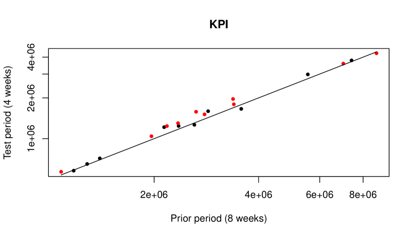
Figure 6: One realization of a single brand simulation. Treatment GEOs are in red, control in black. The reference line is at $y=x/2$ because the test period has half the length of the prior period.

For each simulated data set, weighted least squares regression was used. The weights were proportional to $(1/Y^{\mathrm{pre}})^{2}$, making them inversely proportional to variance. Unweighted regression does not give reliable confidence intervals and $p$-values in this setting.

Some results are plotted in Figure 7 and some numerical summaries are in Table 1. The top panels of Figure 7 show histograms of $1000$ two-sided $p$-values for $H_{0}{:}\beta=0$. This null was rejected $28.6$% of the time for the experiment with a smaller treatment size, and $81.3$% of the time for the one with a larger treatment size. The middle panels show histograms of twice the standard error of $\hat{\beta}$, roughly the distance from $\hat{\beta}$ to the edge of a $95$% confidence interval. At $0.5$% treatment this uncertainty averaged $6.68$ while at $1$% it averaged $3.34$, just over $66$% of the true value $5$. The root mean squared error in $\hat{\beta}$ was $3.21$ for small treatment differences and $1.61$ for large ones. The bottom panels show histograms of the estimates $\hat{\beta}$ for only those simulations in which $H_{0}$ was rejected at the $5$% level. The average estimated effect was $8.64$ for the smaller treatment size and $5.51$ for the larger one.

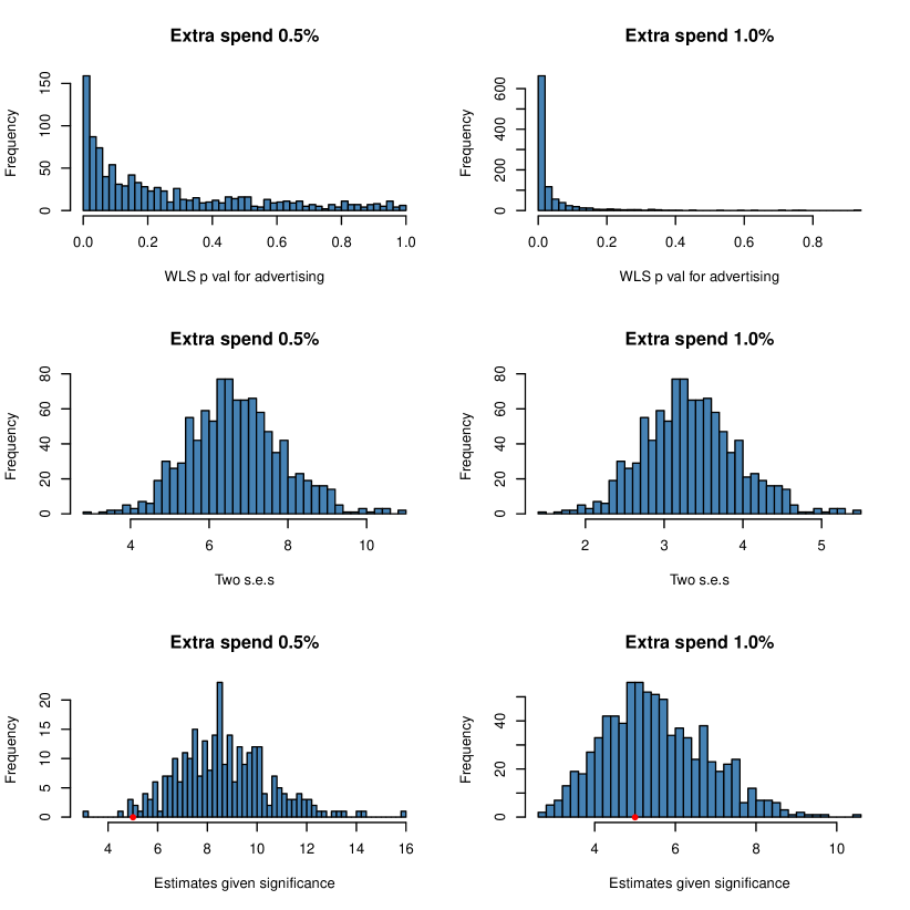
Figure 7: Results from repeated single brand simulations.

The smaller treatment size has very low power, very wide confidence intervals, and in those instances where it detects an advertising effect, it gives a substantial overestimate of effectiveness. The larger treatment size has greater power and only slight overestimation of $\beta$ when it is significant. But it still yields a wide confidence interval for $\beta$.

Trt	$\widehat{\Pr}(p\leq 0.05)$	$2\mathrm{se}(\hat{\beta})$	$\hat{\mathbb{E}}((\hat{\beta}-\beta)^{2})^{1/2}$	$\hat{\mathbb{E}}(\hat{\beta}\mid p\leq 0.05)$
0.5%	0.29	6.68	3.21	8.64
1.0%	0.81	3.34	1.61	5.51

Table 1: Output summary of $1000$ simulations of the single brand experiment.

5 Multibrand experimental results

The multibrand setting was simulated with $B=30$ brands over $G=20$ GEOs. Treatment versus control was assigned with scrambled checker designs from Section 3. The effectiveness of brand $b$ was generated from $\beta_{b}\sim\mathcal{N}(5,1)$, so advertising returns are usually in the range from $3$ to $7$.

5.1 Shrinkage estimation of $\beta_{b}$

We write $\hat{\beta}_{b}$ for the least squares estimate of $\beta_{b}$ from brand $b$ data and set $\hat{\bar{\beta}}=(1/B)\sum_{b=1}^{B}\hat{\beta}_{b}$. We can estimate $\beta_{b}$ by a shrinkage estimator formed as a weighted average of $\hat{\beta}_{b}$ and $\hat{\bar{\beta}}$. Xie et al., (2012, Section 4) propose estimators of the form

$$\tilde{\beta}_{b}=\frac{\lambda}{\mathrm{var}(\hat{\beta}_{b})+\lambda}\hat{\beta}_{b}+\frac{\mathrm{var}(\hat{\beta}_{b})}{\mathrm{var}(\hat{\beta}_{b})+\lambda}\hat{\bar{\beta}}$$ (8)

for a parameter $\lambda$ that must be chosen. The larger $\lambda$ is, the more emphasis we put on brand $b$’s own data instead of the pooled data. For brands with large $\mathrm{var}(\hat{\beta}_{b})$, more weight is put on the pooled estimate $\hat{\bar{\beta}}$. Xie et al.’s (2012) main innovation is in shrinkage methods for data of unequal variances as we have here. To use their method we replace $\mathrm{var}(\hat{\beta}_{b})$ by unbiased estimates $\widehat{\mathrm{var}}(\hat{\beta}_{b})$ taken from the linear model output, and choose $\lambda$.

Xie et al., (2012) give theoretical support for choosing $\lambda$ to minimize the following unbiased estimate of the expected sum of squared errors

$$\begin{split}\mathrm{SURE}^{G}(\lambda)&=\frac{1}{B}\sum_{b=1}^{B}\frac{\mathrm{var}(\hat{\beta}_{b})^{2}}{(\mathrm{var}(\hat{\beta}_{b})+\lambda)^{2}}(\hat{\beta}_{b}-\hat{\bar{\beta}})^{2}\\ &\qquad+\frac{1}{B}\sum_{b=1}^{B}\frac{\mathrm{var}(\hat{\beta}_{b})}{\mathrm{var}(\hat{\beta}_{b})+\lambda}\Bigl{(}\lambda-\mathrm{var}(\hat{\beta}_{b})+\frac{2}{B}\mathrm{var}(\hat{\beta}_{b})\Bigr{)}.\end{split}$$ (9)

This function is not convex in $\lambda$ but a practical way to choose $\lambda$ is to evaluate $\mathrm{SURE}^{G}$ on a grid of, say $1001$, $\lambda$ values. Letting the typical weight on $\hat{\beta}_{b}$ take values $u\in\{0,1/1000,2/1000,\dots,1\}$ we use

$$\lambda=\frac{1}{B}\sum_{b=1}^{B}\mathrm{var}(\hat{\beta}_{b})\times\frac{u}{1-u}$$

where $u=1$ means $\lambda=\infty$ which simply means $\tilde{\beta}_{b}=\hat{\beta}_{b}$.

We can measure the efficiency gain from shrinkage via

$$\mathrm{Eff}=\frac{\frac{1}{B}\sum_{b=1}^{B}(\hat{\beta}_{b}-\beta_{b})^{2}}{\frac{1}{B}\sum_{b=1}^{B}(\tilde{\beta}_{b}-\beta_{b})^{2}}.$$

Figure 8 shows a histogram of this efficiency measure in $1000$ simulations. On average it was about $3.17$ times as efficient to use shrinkage when the experimental treatment is to increase advertising by $1$% of prior sales. For smaller experiments, at $0.5$% of sales, the average efficiency gain was $7.82$. For each given brand $b$, the information from $B-1$ other brands’ data yields a big improvement in accuracy. Recall that $\beta_{b}\stackrel{{\scriptstyle\mathrm{iid}}}{{\sim}}\mathcal{N}(5,1)$. The gain from shrinkage would be less if the underlying $\beta_{b}$ were less similar and greater if they were more similar.

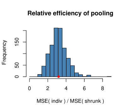
(a) Experimental spend $1$%.

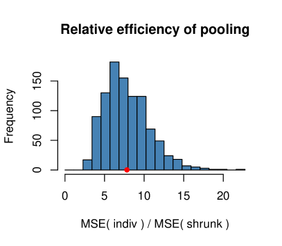
(b) Experimental spend $0.5$%.

Figure 8: Relative efficiency of shrinkage estimates compared to single brand regressions.

5.2 Average return to advertising

The quantity $\bar{\beta}$ measures the overall return to advertising averaged over all brands. Although individual returns $\beta_{b}$ are more informative, their average can be estimated much more reliably. In small experiments where some individual $\hat{\beta}_{b}$’s are not well determined it may be wiser to base decisions on $\hat{\bar{\beta}}$.

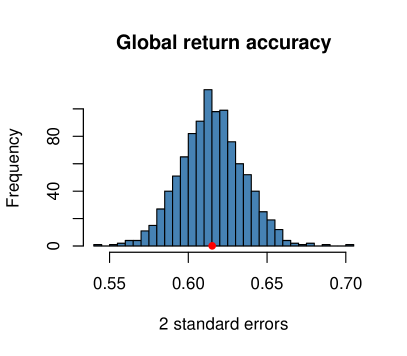
(a) Experimental spend $1$%.

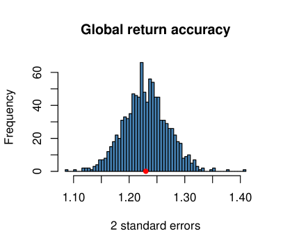
(b) Experimental spend $0.5$%.

Figure 9: Two standard errors of $\hat{\bar{\beta}}$.

We can estimate $\bar{\beta}$ by $\hat{\bar{\beta}}=(1/B)\sum_{b=1}^{B}\hat{\beta}_{b}$ and then using the individual regressions compute $\widehat{\mathrm{var}}(\hat{\bar{\beta}})=B^{-2}\sum_{b=1}^{B}\widehat{\mathrm{var}}(\hat{\beta}_{b})$. Figure 9 shows histograms of $2(\widehat{\mathrm{var}}(\hat{\bar{\beta}}))^{1/2}$. Table 2 compares average values of twice the standard error for $\hat{\beta}$ in a single brand experiment with twice the standard error for $\hat{\bar{\beta}}$ in a multibrand experiment. As we might expect the multibrand standard errors are roughly $\sqrt{B}=\sqrt{30}$ times smaller. Similarly, doubling the spend roughly halves the standard error.

1% spend		0.5% spend
Single	Multiple	Single	Multiple
$3.34$	$0.62$	$6.68$	$1.23$

Table 2: Average over simulations of two standard errors for $\hat{\beta}$ (single brands) and $\hat{\bar{\beta}}$ (multiple brands).

6 Simulation details

In each simulation, the design was generated by the scrambled checker algorithm described in Section 3. Then the data were sampled from the Gamma distributions described here.

6.1 Gamma distributions

The Gamma distribution has a standard deviation proportional to its mean, matching a pattern in the real sales data. When the shape parameter is $\kappa>0$ the Gamma probability density function is ${x^{\kappa-1}e^{-x}}/{\Gamma(\kappa)}$ for $x>0$. To specify a scale parameter, we multiply $X\sim\mathrm{Gam}(\kappa)$ by the desired scale $\theta$.

The random variable $\theta X$ has mean $\kappa\theta$ and variance $\kappa\theta^{2}$, leading to a coefficient of variation equal to $1/\sqrt{\kappa}$ for any $\theta$. The shape $\kappa=1/\mathrm{cv}^{2}$ yields a Gamma random variable with the desired coefficient of variation.

The coefficient of variation for the average of $n$ observations from one GEO (e.g., $n_{\mathrm{post}}=4$ in the test period and $n_{\mathrm{pre}}=8$ in the background period) is approximately $1/\sqrt{n}$ times the coefficient of variation of a single observation. The coefficient of variation for single observations from a set of $8$ week trial periods was about $0.15$ while that for $4$ week followup periods was about $0.1$. These figures are based on aggregates over GEOs that were very similar for all of the different brands. An $8$ week trial period has within it more seasonality than a $4$ week period has, and so it is reasonable that we would then measure a larger coefficient of variation.

To simulate with a specific coefficient of variation we use $\kappa=n/\mathrm{cv}^{2}$. This leads to $\kappa_{\mathrm{pre}}=8/0.15^{2}\doteq 356$ and $\kappa_{\mathrm{post}}=4/0.1^{2}=400$.

Gamma random variables are never negative which gives them a further advantage over simulations with Gaussian random variables. For the specific parameter choices above, the shape parameters are large enough that the Gamma random variables are not strongly skewed (their skewness is $2/\sqrt{\kappa}$). A Gaussian distribution might give similar results. The Gamma distribution is useful because it can be used to simulate either strongly or mildly skewed data that are always nonnegative.

6.2 Data generation

For a single brand experiment, the data are generated as follows. First the underlying sizes of the GEOs were sampled as $S_{g}=10^{7-U_{g}}$ where $U_{g}\sim\mathbf{U}(0,\phi)$, for $g=1,\dots,G$. The quantity $S_{g}$ is interpreted as a size measure for GEO $g$. We will use it as the expected prior sales, which is then roughly proportional to the number of customers in GEO $g$. Choosing $\phi=1$ means that we consider GEOs ranging in size by a factor of about $10$ from largest to smallest.

The prior KPIs are generated as

$$Y_{g}^{\mathrm{pre}}\stackrel{{\scriptstyle\mathrm{ind}}}{{\sim}}S_{g}\times{\mathrm{Gam}(\kappa_{\mathrm{pre}})}/{\kappa_{\mathrm{pre}}},$$

where $\kappa_{\mathrm{pre}}=n_{\mathrm{pre}}/\mathrm{cv}_{\mathrm{pre}}^{2}$. Then $\mathbb{E}(Y_{g}^{\mathrm{pre}})=S_{g}$. Let the spending level in the experimental period be $X_{g}^{\mathrm{post}}$ in GEO $g$. Then the KPI in the experimental period is generated as

$$Y_{g}^{\mathrm{post}}\stackrel{{\scriptstyle\mathrm{ind}}}{{\sim}}\frac{n_{\mathrm{post}}}{n_{\mathrm{pre}}}\times S_{g}\times\mathrm{Gam}(\kappa_{\mathrm{post}})/\kappa_{\mathrm{post}}+X_{g}^{\mathrm{post}}\beta,$$

where $\kappa_{\mathrm{post}}=n_{\mathrm{post}}/\mathrm{cv}_{\mathrm{post}}^{2}$. The factor $n_{\mathrm{post}}/n_{\mathrm{pre}}$ adjusts for different sizes of prior and experimental observation windows. The term $X_{g}^{\mathrm{post}}\beta$ is the additional KPI attributable to advertising.

6.3 Checkerboard designs

The scrambled checkerboard design was run for $2\times G\times B\times 25=30{,}000$ steps. The expected number of flips for each pixel in the image is $25$. This is much more than the number at which the root mean squared correlations stabilize.

7 A fully Bayesian approach

Stein shrinkage is an empirical Bayes approach. Here we consider a fully Bayesian alternative. When it comes to pooling information together from observations that arise from a common model but corresponding to different sets of parameters, Bayesian hierarchical models arise as a natural solution.

One advantage of the Bayesian approach is that it allows us to present the uncertainty in our estimates. For each brand $b$, we can get an interval $(L_{b},U_{b})$ such that $\Pr(L_{b}\leq\beta_{b}\leq U_{b}\mid\text{data})=0.95$ without making any (additional) assumptions. These posterior credible intervals are easier to compute than confidence intervals from Stein shrinkage. We can also use posterior credible intervals at the planning stage. To do that, we simulate the data several times and record how wide the posterior credible intervals are. If they are too wide we might add more GEOs or increase the differential spend $\delta$.

7.1 A hierarchical model

We consider model (2) in a Bayesian context, which translates as follows:

$$\mu_{gb} :=\alpha_{0b}+\alpha_{1b}Y^{\mathrm{pre}}_{gb}+\beta_{b}X_{gb}^{\mathrm{post}},\quad b=1,\dots,B,\ g=1,\dots,G$$ (10)

$$Y^{\mathrm{post}}_{gb} \sim\mathcal{N}\Bigl{(}\mu_{gb},\bigl{(}{\sigma_{b}}/{Y^{\mathrm{pre}}_{gb}}\bigr{)}^{2}\Bigr{)},\quad b=1,\dots,B,\ g=1,\dots,G$$ (11)

$$\sigma_{b}^{2} \sim\mathcal{IG}(10^{-3},10^{-3}),\quad b=1,\dots,B$$ (12)

$$\beta_{b} \sim\mathcal{N}(\beta,\sigma_{\beta}^{2}),\quad b=1,\dots,B$$ (13)

$$\sigma_{\beta}^{2} \sim\mathcal{IG}(0.5,0.5),\quad\text{and},$$ (14)

$$\beta \sim{\boldsymbol{1}}_{\mathbb{R}}.$$ (15)

Definitions (10), (11) and (12) the mirror model (2) that we described earlier. Notice that we signal the weighted regression explicitly in (11). The hierarchical Gaussian prior (13) on the coefficients $\beta_{b}$ involves two new hyperparameters $\beta$ and $\sigma_{\beta}^{2}$ which respectively represent the overall mean and variance of all returns $\beta_{b}$. Since we assumed in the beginning that all brands had somewhat similar returns, we choose a semi-informative prior (14) on $\sigma_{\beta}^{2}$ that favors plausible, not too large, values. For our simulations we use a flat prior (15) on $\beta$ relying on the data to drive the inference. One could also use a Gaussian prior for $\beta$, crafting its mean and variance based on the prior knowledge of the brands at hand.

7.2 Simulation details

The data were generated according to the procedures described in Section 6. Samples were collected from the posterior distribution using STAN software (Stan Development Team,, 2016).

We simulated many different conditions and consistently found that the Stein and Bayes estimates were close to each other. In this section we present just one simulation matching parameters of interest to some of our colleagues at Google. We consider $G=160$ GEOs, only $B=4$ brands and we take advertising effectiveness $\beta_{b}$ to be $\mathcal{N}(1,1)$. Using $\mathbb{E}(\beta_{b})=1$ produces a setting where a dollar of advertising typically brings back a dollar of sales in the observation period. That implies a short term loss with an expected longer term benefit from adding or retaining customers. Taking the standard deviation of $\beta_{b}$ to one implies very large brand to brand variation. We still see a benefit from pooling only $4$ brands as diverse as that. The amount of extra spend is set to $1$% of prior sales ($\delta=0.01$). We repeated this simulation $1000$ times.

In this setting with $160$ GEOs and $4$ brands there will always be some GEOs that get the exact same treatment for all $4$ brands.

7.3 Agreement with shrinkage estimates

Figure 10 compares the RMSE $[(1/B)\sum_{b=1}^{B}(\hat{\beta}_{b}-\beta_{b})^{2}]^{1/2}$ for Stein and Bayes estimation in $1000$ simulations with $B=4$. The methods have very similar accuracy. For high brand to brand standard deviation $\sigma_{b}=1.0$, there is a slight advantage to Bayes. For lower brand to brand standard deviation $\sigma_{b}=0.25$, there is a small advantage to Stein. The Bayesian estimate was at a disadvantage there because the prior variance was $1/\mathrm{Gamma}(0.5,0.5)$ giving $\sigma_{b}$ a median of about $1.48$. This shows that the Bayesian estimate is not overly sensitive to our widely dispersed prior distribution on $\sigma_{b}$.

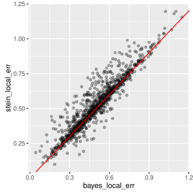
(a) Stein versus Bayes RMSE, $\sigma_{b}=1$.

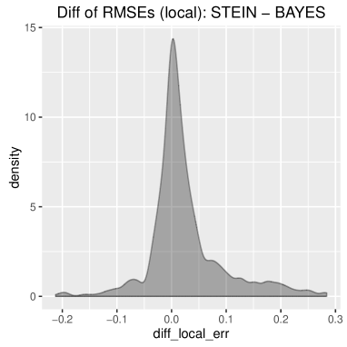
(b) Stein minus Bayes RMSE, $\sigma_{b}=1$.

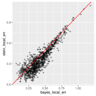
(c) Stein versus Bayes RMSE, $\sigma_{b}=0.25$.

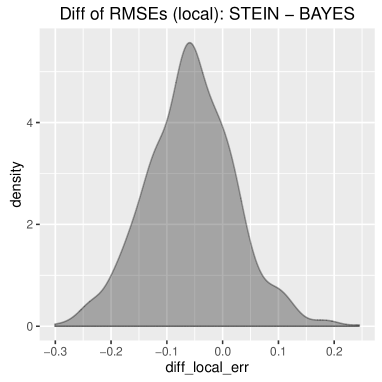
(d) Stein minus Bayes RMSE, $\sigma_{b}=0.25$.

Figure 10: Comparison of Bayes and Stein RMSEs on two simulations of $1000$ replicates with $B=4$ brands.

7.4 Posterior credible intervals

To investigate what power can be gained pooling data together using a multibrand experiment over conducting multiple single-brand experiments independently, we simulated datasets following the same procedure as before, using $G=160$ GEOs with either $B=1$ (no pooling) or $B=4$ (pooling) brands, the effectivenesses of which were drawn from a Gaussian distribution $\mathcal{N}(1,\sigma^{2}_{b})$ with $\sigma_{b}=0.25$. Now the brands return on average one dollar of incremental revenue per dollar spent, and the standard deviation of $0.25$ represents substantial brand differences. The relative incremental ad-spend we made varies from 0.5% to 2% to show how it impacted the results. Figure 11 displays the estimated densities (over 10,000 replications) of the half-width of 95% credible intervals around the brands’ effectivenesses, the solid lines representing the 95% quantile of these densities, in each scenario.

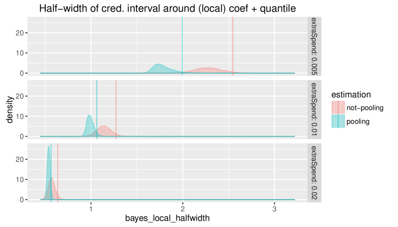
Figure 11: Distribution of the half-width of credible intervals around brands’ effectiveness coefficients.

While the half-width of credible intervals does not quite display an inverse relationship with the extra spend when pooling multiple experiments together as it does when conducting experiments separately (doubling the incremental spend lets us detect twice as small an effectiveness in the single-brand scenario), it is clear that pooling experiments together does bring improvement to the power of the geoexperiments.

It is best if posterior credible intervals have frequentist coverage levels close to their nominal values. Table 3 shows empirical coverage levels for $B=4$ brands and $G=160$ GEOS for a range of average returns $\beta$ and brand to brand standard deviations $\sigma_{b}$. On the whole the coverage is quite close to nominal. There is slight over coverage, probably due to the prior being dominated by large values of $\sigma_{b}$.

$\beta\bigm{\backslash}{\sigma_{b}}$	0.10	0.25	0.50	0.75	1.00
0.25	0.974	0.974	0.967	0.953	0.950
0.50	0.975	0.967	0.962	0.954	0.946
0.75	0.974	0.968	0.967	0.959	0.952
1.00	0.978	0.975	0.969	0.964	0.954
1.25	0.975	0.968	0.966	0.960	0.958
1.50	0.978	0.968	0.966	0.954	0.954

Table 3: Observed coverage levels of 95% Bayesian credible intervals. Six values of average gain $\beta$ and five values of brand standard error $\sigma_{b}$.

8 Conclusions and discussion

In our examples we see that combining data from multiple brands at once leads to more accurate experiments than single brand experiments would yield. This happens for both Bayes and empirical Bayes (Stein shrinkage) estimates. The estimate for any given brand gets better by using data from the other brands.

This efficiency brings practical benefits. An experiment on multiple brands might need to use fewer GEOs, or it might be informative at smaller, less disruptive, changes in the amount spent.

Ordinary Stein shrinkage towards a common mean is advantageous when $B\geq 4$ by the theory of Stein estimation (Efron and Morris,, 1973). The method of Xie et al., (2012) is further optimized to handle unknown and unequal variances.

We have simply plugged in unbiased estimates of variance. Hwang et al., (2009) propose a different method that begins with shrinkage applied to the variance estimates themselves. They also develop confidence intervals that could be used for our $\beta_{b}$. Stein shrinkage is a form of empirical Bayes estimation. We found that by using a Bayesian hierarchical model we could get posterior credible intervals with good frequentist coverage.

For planning purposes it is worthwhile to consider what parameter values are realistic in a specific setting. By simulating several choices we can find an experiment size that gets the desired accuracy at acceptable cost.

The most difficult quantity to choose for a simulation is $\sigma_{b}^{2}$, the variance of the true returns $\beta_{b}$ to advertising for different brands. That is difficult because one often starts from a position of not having good causal values for any individual brand. One more values for this parameter must then be chosen based on intuition or opinion. Because the true response rate to advertising can be expected to drift it is reasonable to suppose that multiple experiments will need to be made in sequence. Estimates of $\sigma^{2}_{b}$ from one experiment will be useful in planning the next ones.

References

- Cochran and Cox, (1957) Cochran, W. G. and Cox, G. M. (1957). Experimental designs. John Wiley & Sons, New York.
- Diaconis and Gangolli, (1995) Diaconis, P. and Gangolli, A. (1995). Rectangular arrays with fixed margins. In Aldous, D., Diaconis, P., Spencer, J., and Steele, J. M., editors, Discrete probability and algorithms, volume 72. Springer, New York.
- Djoković et al., (2014) Djoković, D. Z., Golubitsky, O., and Kotsireas, I. S. (2014). Some new orders of Hadamard and skew-Hadamard matrices. Journal of combinatorial designs, 22(6).
- Efron, (2008) Efron, B. (2008). Row and column correlations:(are a set of microarrays independent of each other?). Technical report, Stanford University, Division of Biostatistics.
- Efron and Morris, (1973) Efron, B. and Morris, C. (1973). Stein’s estimation rule and its competitors—an empirical Bayes approach. Journal of the American Statistical Association, 68(341):117–130.
- Hedayat et al., (2012) Hedayat, A. S., Sloane, N. J. A., and Stufken, J. (2012). Orthogonal arrays: theory and applications. Springer, New York.
- Hwang et al., (2009) Hwang, J. T. G., Qiu, J., and Zhao, Z. (2009). Empirical Bayes confidence intervals shrinking both means and variances. Journal of the Royal Statistical Society, Series B, 71(1):265–285.
- Satterthwaite, (1959) Satterthwaite, F. E. (1959). Random balance experimentation. Technometrics, 1(2):111–137.
- Stan Development Team, (2016) Stan Development Team (2016). Stan Modeling Language User’s Guide and Reference Manual, Version 2.12.0.
- Vaver and Koehler, (2011) Vaver, J. and Koehler, J. (2011). Measuring ad effectiveness using geo experiments. Technical report, Google Inc.
- Vaver and Koehler, (2012) Vaver, J. and Koehler, J. (2012). Periodic measurement of advertising effectiveness using multiple-test-period geo experiments. Technical report, Google Inc.
- Xie et al., (2012) Xie, X., Kou, S. C., and Brown, L. D. (2012). SURE estimates for a heteroscedastic hierarchical model. Journal of the American Statistical Association, 107(500):1465–1479.