Spatial Distribution of Mg-Rich Ejecta in LMC Supernova Remnant N49B

Abstract

The supernova remnant (SNR) N49B in the Large Magellanic Cloud is a peculiar example of a core-collapse SNR to show the shocked metal-rich ejecta enriched only in Mg without evidence for a similar overabundance in O and Ne. Based on archival Chandra data we present results from our extensive spatially-resolved spectral analysis of N49B. We find that the Mg-rich ejecta gas extends from the central regions of the SNR out to the southeastern outermost boundary of the SNR. This elongated feature shows an overabundance for Mg similar to that of the main ejecta region at the SNR center, and its electron temperature appears to be higher than the central main ejecta gas. We estimate that the Mg mass in this southeastern elongated ejecta feature is $\sim$10% of the total Mg ejecta mass. Our estimated lower limit of $>$0.1 $M_{\odot}$ on the total mass of the Mg-rich ejecta confirms the previously-suggested large mass for the progenitor star ($M$ $\mathrel{\hbox{\hbox to0.0pt{\hbox{\lower 4.0pt\hbox{$\sim$}}\hss}\hbox{$>$}}}$ 25 $M_{\odot}$). We entertain scenarios of an SNR expanding into a non-uniform medium and an energetic jet-driven supernova in an attempt to interpret these results. However, with the current results, the origins of the extended Mg-rich ejecta and the Mg-only-rich nature of the overall metal-rich ejecta in this SNR remain elusive.

1. INTRODUCTION

N49B is an X-ray-bright supernova remnant (SNR) in the Large Magellanic Cloud (LMC). The presence of a nearby H II region (Chu & Kennicutt, 1988) and a molecular cloud (Cohen et al., 1988) suggested a core-collapse supernova (SN) explosion of a massive star for the origin of N49B. The shock expansion in an interstellar cavity was suggested by the ASCA data (Hughes et al., 1998), which was supportive of its massive progenitor star. Based on Chandra data we detected a large variation in the surface brightness of the swept-up interstellar medium (ISM), which indicates that the SNR is expanding into an ambient medium with an order of magnitude density variation along the outer boundary of the SNR, generally consistent with the shock interaction with nearby molecular clouds (Park et al. 2003b, , P03 hereafter). The Chandra data allowed us to detect the shocked metal-rich ejecta in N49B for the first time (P03). The detected metal-rich ejecta gas is enriched only in Mg, and the estimated large mass for the Mg-rich ejecta gas firmly established a very massive progenitor, and thus a core-collapse origin for N49B (P03). The putative compact stellar remnant has not been detected, and a 3$\sigma$ upper limit on the central source luminosity ($L_{0.5-5keV}$ $<$ 2 $\times$ 10³³ erg s^-1) was placed based on the Chandra data (P03).

It is notable that only two SNRs, including N49B, (out of $\sim$500 SNRs detected in the Galaxy and Magellanic Clouds) show this characteristic Mg-overabundance (while no other metal elements are similarly enhanced): the Galactic SNR G284.3–1.8 is the other member of this peculiar group (Williams et al., 2015). The true nature and origin of the only-Mg-rich ejecta in these SNRs are unclear. It might have resulted from a peculiar core-collapse nucleosynthesis, or a particular thermal condition in the ejecta gas might be responsible for the observed Mg line enhancement. If the observed Mg-rich nature (without enhancements in O and Ne) represents the true metal abundance structure in these SNRs, it may challenge the standard core-collapse nucleosynthesis models in which an invariably larger amount of O and Ne (than Mg) is expected to be created (e.g., Thielemann et al., 1996; Nomoto et al., 2006). N49B is particularly important to study this rare group of SNRs because it appears that the bulk of the shocked Mg-rich ejecta gas has been detected (whereas the Mg-rich ejecta in G284.3–1.8 is detected in a small part of the SNR). The detection of the entire Mg-rich ejecta in N49B allows us a unique opportunity to study the overall nature of the ejecta, such as the total shocked ejecta mass and its spatial structure, in this peculiar SNR.

We here report the presence of an emission feature in N49B, extending from the central ejecta regions out to the southeastern outer boundary of the SNR. This elongated region is enriched only in Mg just like the bulk of the metal-rich ejecta gas in the central region of the SNR. This extended Mg-rich emission feature was hinted at by the Mg line equivalent width (EW) image in the previous Chandra data analysis (P03), but was not discussed in P03. In this work we focus on the spectral and morphological properties of this particular feature. We present the data and data analysis in Sections 2 & 3, respectively. In Section 4 we discuss the nature of the elongated Mg-rich ejecta.

2. DATA

N49B was observed with the S3 chip of the Advanced CCD Imaging Spectrometer (ACIS) on board Chandra on 2001 September 15 as part of the Guaranteed Time Observation program (P03). We reprocessed these archival Chandra data (ObsID 1041) of N49B (using CIAO version 4.2 with CALDB version 4.3.0). We processed the raw event file following the standard data reduction methods which include the correction for the charge transfer inefficiency. We applied the standard data screening by event status and grade (ASCA grades 02346). As noted by P03 the overall light curve from the entire S3 chip shows a moderately enhanced particle background (by a factor of $\sim$2 above the average quiescent count rate) for the last $\sim$10% of the exposure. We excluded this part of the data ($\sim$4-ks time interval) from our analysis. After the data reduction the total effective exposure is $\sim$30.2 ks.

3. ANALYSIS & RESULTS

3.1. Mg Enhancement in Southeastern Region

The broadband ACIS image of N49B shows a nearly circular overall morphology with several relatively bright filaments located mostly around the outer boundary of the SNR (Figure 1a). The central regions of N49B, in which X-ray emission is dominated by the shocked Mg-rich ejecta (P03), are generally faint and diffuse without showing any well-organized emission feature (corresponding to the Mg-enhanced regions). The Mg-rich ejecta gas was identified aided by a Mg K$\alpha$ line (at $E$ $\sim$ 1.35 keV) EW image (P03). In Figure 1b we reproduce the Mg line EW image of N49B as was presented in P03. To create Figure 1b we followed the same methods used by P03 (and references therein). We used the same photon energy bands for the Mg K$\alpha$ line ($E$ = 1280 – 1440 eV), and for the adjacent continuum ($E$ = 1140 – 1240 and 1550 – 1700 eV, to estimate the underlying continuum flux) as those selected by P03. While the bright Mg line EW in the central region of the SNR is evident, the enhanced Mg line clearly extends to the southeast (region E in Figure 1b). This enhanced line EW feature is elongated ($\sim$20^′′ in thickness and $\sim$65^′′ in length), extending from the central Mg-rich ejecta region out to the outermost southeastern boundary of the SNR. This feature was hinted at in Figure 2 of P03 (although it appeared to be less clear than that in Figure 1b, probably due to a different smoothing method adopted by P03), but it was not discussed by P03 as they focused on the detection of the central Mg-rich ejecta.

To quantitatively assess the apparently Mg-enhanced nature of this region we extracted the observed X-ray spectrum from region E (as shown in Figure 1). The X-ray emission in this region contains $\sim$7300 counts in the 0.4 – 5 keV band. We binned the extracted spectrum to contain at least 20 counts per photon energy channel. We fit this spectrum with a non-equilibrium ionization (NEI) plane shock model (vpshock in XSPEC, Borkowski et al. 2001). We used NEI version 2.0 in XSPEC, associated with ATOMDB (Foster et al., 2012) which includes inner-shell lines (from Li-like ions) and updated Fe-L shell transition lines (see Badenes et al., 2006). We note that the plane shock model used by P03 did not include these additional X-ray lines which could affect the estimates of the thermal parameters (and thus elemental abundances) for an under-ionized gas. In these spectral model fits we assumed two components for the foreground absorbing column: one for the Galactic absorption toward the LMC ($N_{H,Gal}$) and the other for the LMC column ($N_{H,LMC}$). We fixed $N_{H,Gal}$ at 6 $\times$ 10²⁰ cm^-2 (Dickey & Lockman, 1990) with solar abundances (Anders & Grevesse, 1989). We fitted $N_{H,LMC}$ assuming the LMC abundances (Russell & Dopita, 1992; Schenck et al., 2016).

For the plane shock component we initially fixed all elemental abundances at the LMC values: i.e., He = 0.89, C = 0.303, N = 0.123, Ar = 0.537, Ca = 0.339, Ni = 0.618 (Russell & Dopita, 1992), and O = 0.13, Ne = 0.20, Mg = 0.20, Si = 0.28, S = 0.31, Fe = 0.15 (Schenck et al., 2016). Abundances are with respect to solar values (Anders & Grevesse, 1989), hereafter. We fixed the redshift parameter at $z$ = 9.54 $\times$ 10^-4 for the radial velocity of the LMC (Meaburn et al., 1995). The electron temperature ($kT$, where $k$ is the Boltzmann constant) and ionization timescale ($\tau$ = $n_{e}t$, where $n_{e}$ is the electron density and $t$ is the time since the gas has been shocked) are varied. The normalization parameter (a scaled volume emission measure, EM = $n_{e}$$n_{H}$$V$, where $n_{H}$ is the H density and $V$ is the emission volume) is also varied. The fit is statistically unacceptable ($\chi^{2}_{\nu}$ $\sim$ 2.4) due to large residuals around the Mg K line feature ($E$ $\sim$ 1.35 keV). Also, there is significant excess emission at $E$ $\mathrel{\hbox{\hbox to0.0pt{\hbox{\lower 4.0pt\hbox{$\sim$}}\hss}\hbox{$>$}}}$ 2 keV above the best-fit model ($kT$ $\sim$ 0.6 keV). The observed X-ray spectrum in this high energy tail shows negligible (or very weak) K-shell line emission features from S ($E$ $\sim$ 2.4 – 2.6 keV), Ar ($E$ $\sim$ 3.1 – 3.3 keV), and Ca ($E$ $\sim$ 3.9 – 4.1 keV).

Varying the Mg abundance significantly improves the fit ($\chi^{2}_{\nu}$ $\sim$ 1.4), and the best-fit Mg abundance is $\sim$0.52, higher than the LMC value by a factor of $\sim$2.6, suggesting the presence of overabundant Mg. When we additionally varied abundances for O, Ne, Si, and Fe (whose K- and/or L-shell transition lines are prominent in our fitted 0.4 – 5.0 keV band), the statistical improvement of the model fit is not significant ($\chi^{2}_{\nu}$ $\sim$ 1.3). The best-fit Mg abundance does not change (Mg = 0.52), while all other fitted abundances are consistent with the LMC values within uncertainties. It is notable that, even with varying abundances, the significant excess emission at $E$ $\mathrel{\hbox{\hbox to0.0pt{\hbox{\lower 4.0pt\hbox{$\sim$}}\hss}\hbox{$>$}}}$ 2 keV is evident for the best-fit electron temperature $kT$ $\sim$ 0.6 keV. Thus, although the best-fit one-temperature model may be considered to be statistically acceptable ($\chi^{2}_{\nu}$ $\sim$ 1.3 – 1.4), we added another NEI plane shock component in our spectral model to properly fit the excess emission at $E$ $>$ 2 keV. For the two-component model fit we initially fixed all metal abundances at the LMC values for both components, while varying other model parameters. The fit is statistically unacceptable ($\chi^{2}_{\nu}$ $\sim$ 2.0). It is clear that the best-fit model underestimates the strong Mg line at $E$ $\sim$ 1.35 keV. All other emission line features are adequately fitted. The bulk of X-ray emission at $E$ $\mathrel{\hbox{\hbox to0.0pt{\hbox{\lower 4.0pt\hbox{$\sim$}}\hss}\hbox{$<$}}}$ 1 keV is fitted by the K lines from H- and He-like O and Ne ions (and some L-shell transition lines from Fe ions) with the LMC-like abundances. Thus, we fixed all metal abundances at the LMC values for the soft component assuming that this component is dominated by the emission from the shocked LMC ISM. We consider the hard component spectrum to originate primarily from the shocked Mg-rich ejecta, and thus varied the Mg abundance (with all other elements being fixed at the LMC abundances) for the hard component. The model fit significantly improves ($\chi^{2}_{\nu}$ $\sim$ 1.0). The best-fit Mg abundance for the hard component ($kT_{hard}$ $\sim$ 1.55 keV) is 0.93. These results are summarized in Table 1. The observed spectrum of region E (with this best-fit two-component plane shock model overlaid) is shown in Figure 2. In these spectral model fits of the region E spectrum we assumed the recent measurements of the LMC abundances for O, Ne, Mg, Si, and Fe (except for the Mg abundance in the ejecta component spectrum) based on the Chandra data of the LMC SNRs (Schenck et al., 2016), while we adopted LMC abundance values by Russell & Dopita (1992) for other elements. We note that, for the LMC abundances, several measurements are available in the literature (e.g., Russell & Dopita, 1992; Hughes et al., 1998; Davies et al., 2015; Maggi et al., 2016; Schenck et al., 2016). There are some inconsistencies (up to by a factor of $\sim$2) among those abundance measurements, whose origins are not fully understood: e.g., the cross-calibrations over different wavelengths and instruments, the use of different objects (stars, SNRs, HII regions), the model dependence of measurements, etc. We find no considerable effects on our spectral model fits depending on the choice of a specific LMC abundance set. The fitted parameters are consistent within statistical uncertainties with equally-good fits: e.g., assuming the higher (and more traditional) values of the LMC abundances (O = 0.26, Ne = 0.33, Si = 0.31, Mg = 0.32 and Fe = 0.36) measured by Russell & Dopita (1992), we find that the Mg abundance for the hard (ejecta) component is 1.12${}^{+0.12}_{-0.11}$ with a nearly the same electron temperature ($kT$ $\sim$ 1.54 keV), ionization timescale ($\tau$ $\sim$ 0.7 $\times$ 10¹¹ cm^-3 s), and the volume emission measure ($\sim$0.5 $\times$ 10⁵⁸ cm^-3) as listed in Table 1. For all other regional spectral analysis as presented in Section 3.2, we fit the ISM abundances for O, Ne, Mg, Si, and Fe in our spectral model fits, while fixing other elemental abundances at values by Russell & Dopita (1992).

When we varied abundances for O, Ne, Si, and Fe (as well as Mg) in the hard component plane shock model fit, the statistical goodness-of-the-fit is nearly the same ($\chi^{2}_{\nu}$ $\sim$ 1.0) with similar main results: i.e., Mg is overabundant ($\sim$1.5) with a high electron temperature ($kT$ $\sim$ 4 keV). The Ne abundance appears to be elevated ($\sim$0.7) with a negligible Fe abundance ($<$0.04). These Ne and Fe abundances are somewhat different than those presented in Table 1, and are potentially interesting to reveal the true nature of the ejecta composition and the SN nucleosynthesis of this SNR. However, the statistical improvement of this model fit is negligible, compared to that with the LMC abundances for those elements. Nonetheless, these (possibly non-LMC like) Ne and Fe abundances do not affect our conclusions on the Mg-rich ejecta in region E. Finally, we considered a power law (PL) spectrum to fit the high energy tail of the region E spectrum. The model fit (plane shock + PL) is statistically good ($\chi^{2}_{\nu}$ $\sim$ 0.9). The Mg overabundance is evident ($\sim$0.92) with LMC-like abundances for all other fitted elements, but a low temperature ($kT$ $\sim$ 0.34 keV) is implied for the Mg-rich ejecta gas. The best-fit PL photon index ($\Gamma$ $\sim$ 2.4) is consistent with that for the synchrotron radiation from relativistically-accelerated shocked electrons in the shell-type SNR N49B (Dickel & Milne, 1998). However, the radio data of N49B show the lack of such non-thermal emission generally in the southern regions of the SNR (Dickel & Milne, 1998), particularly in regions corresponding to region E (see Section 4). We consider that the physical origin of this phenomenologically-motivated PL model component is uncertain, and that the main results of the Mg-rich ejecta for region E are persistent. In the following discussion of region E, we assume the best-fit parameters from our two-component plane shock model fit with the LMC abundances for metal elements other than Mg (as presented in Table 1), unless noted otherwise.

3.2. Central Ejecta and Ambient Gas

We performed a similar spectral analysis of central Mg-rich ejecta regions. To characterize thermal condition and metal abundance for the central ejecta region, we extracted X-ray spectra from regions A – D as marked in Figure 1. We selected these regions to represent all characteristic subregions showing the strong Mg line EW, while achieving significant photon count statistics of $\mathrel{\hbox{\hbox to0.0pt{\hbox{\lower 4.0pt\hbox{$\sim$}}\hss}\hbox{$>$}}}$5000 counts per region. We fit these regional spectra with the NEI plane shock model generally following the method described in Section 3.1. As expected these regional spectra cannot be fitted by the LMC abundances ($\chi^{2}_{\nu}$ $\sim$ 3 – 5) because of the significant discrepancy between the spectral model and the observed spectrum for the strong Mg K emission line feature. Varying the Mg abundance results in statistically acceptable fits ($\chi^{2}_{\nu}$ $\sim$ 0.9 – 1.3) for all four regional spectra. We note that, in contrast to region E, there is no excess emission above the best-fit model at $E$ $\mathrel{\hbox{\hbox to0.0pt{\hbox{\lower 4.0pt\hbox{$\sim$}}\hss}\hbox{$>$}}}$ 2 keV for these central regions. The best-fit Mg abundance is significantly higher than the LMC value (by a factor of $\sim$4–6) for all four regions. While the LMC abundances for O, Ne, Si, and Fe can adequately fit the observed spectra of these central regions, for the purposes of statistical comparisons of metal abundances among the central ejecta regions and the shocked ISM regions, we fitted abundances for O, Ne, Si, and Fe as well as Mg in this work. As perhaps expected, best-fit abundances for O, Ne, Si, and Fe are consistent with the LMC values within statistical uncertainties, except for the moderately elevated Si abundance in region A (by a factor of $\sim$2 above the LMC abundance). We summarize these results in Tables 2 & 3. In Figure 3 we show the observed spectra (with the best-fit NEI plane shock model overlaid) for regions A – D.

We extract spectra from thirteen regions (regions 1 – 13 in Figure 1) for which our Mg EW image shows no enhancements. X-ray emission in these regions presumably originates from the shocked ISM with LMC-like abundances (P03). We selected these regions to characteristically represent bright filaments and faint diffuse regions (in the broadband image) exterior to the enhanced Mg EW regions, while achieving significant photon statistics of $\mathrel{\hbox{\hbox to0.0pt{\hbox{\lower 4.0pt\hbox{$\sim$}}\hss}\hbox{$>$}}}$4000 counts in the 0.4 – 5 keV band. The observed X-ray spectra of these regions show weak atomic emission line features for all metal elements in contrast to regions A – E in which a strong Mg line emission feature is evident. We show four example regional spectra from these shocked ISM-dominated regions in Figure 4. We performed the NEI plane shock model fits to these regional spectra with all metal abundances fixed at the LMC values. These model fits are acceptable with $\chi^{2}_{\nu}$ $\sim$ 0.8 – 1.4. When we varied metal abundances for O, Ne, Mg, Si, and Fe, fits are nearly the same ($\chi^{2}_{\nu}$ $\sim$ 0.8 – 1.3) with similar best-fit values for the fitted parameters. Although these regional spectra can be fitted with metal abundances fixed at the LMC values, for the purposes of statistical comparisons with the ejecta-dominated regions, we use the results based on our spectral model fits with elemental abundances varied in this work.

Region 13 contains very faint outermost filaments in which we detect only $\sim$700 counts. Our best-fit NEI plane shock model fit for this regional spectrum shows generally similar results to those for other ISM regions. However, because of significantly poorer photon count statistics in this regional spectrum, uncertainties on the best-fit values of the model parameters are large, and the measurements are less reliable for this region. Thus, we do not present the quantitative measurements of our fitted spectral model parameters for this region. Regions 5 and 10 also include relatively lower count statistics of $\sim$2000 counts. Our spectral model fits for these regions do not allow a unique solution, and result in large uncertainties on the best-fit values. Spectra from these regions can be equally described by a few different NEI plane shock model fits after fixing some parameters (e.g., $N_{H,LMC}$ and $kT$) at the mean values of the neighboring regions. Since results from those model fits are consistent (within uncertainties), we present average values of the best-fit parameters between these alternative model fits for these two regions. These results are in agreement with those from other shocked ISM regions. We summarize these results in Tables 2 & 3.

4. DISCUSSION

Our spectral analysis of the observed X-ray spectra for a number of subregions in N49B shows that Mg is clearly overabundant in regions A – E when compared to that in ISM-dominated regions (Figure 5). In contrast to Mg the estimated abundances for other metal elements (O, Ne, Si, and Fe) are consistent with the LMC values throughout the entire SNR (Figures 5 & 6). This Mg-only enhancement is consistently observed for region E in addition to regions A – D. The electron temperature and ionization timescale show similar ranges between the ejecta and ISM regions (probably except for region E, Figure 7), suggesting that the observed enhancements in the Mg line EW in N49B are primarily due to the Mg overabundance. It is remarkable that X-ray emission from the shocked Mg-rich ejecta gas apparently extends from the central ejecta regions (regions A – D) out to the southeastern outermost boundary of the SNR. This extended Mg-rich ejecta gas is confined in an elongated region (region E in Figure 1), presumably with a cylindrical geometry. The Mg abundance in this region is estimated to be higher than the LMC abundance by a factor of $\sim$5, which is consistent with the Mg overabundance detected in the central regions of this SNR. It is interesting to find that the Mg-rich ejecta gas in region E shows a significantly higher temperature ($kT$ $\sim$ 1.6 keV) than that of the central ejecta gas ($kT$ $\sim$ 0.6 keV) (Figure 7). The Mg overabundance and high electron temperature in region E are persistent between the northern and southern halves of region E (although larger uncertainties are implied for the best-fit values due to lower count statistics in these half-regions). Thus, region E likely represents a continuous outflow of the hot Mg-rich ejecta gas channeled from the SNR center to the outermost boundary of the SNR.

P03 estimated a large mass of the Mg-rich ejecta ($\mathrel{\hbox{\hbox to0.0pt{\hbox{\lower 4.0pt\hbox{$\sim$}}\hss}\hbox{$>$}}}$1 $M_{\odot}$) for N49B, extrapolating the measured Mg abundance in a small Mg-enhanced region near the SNR center (roughly corresponding to the southern half of region A) to the entire Mg-enhanced region in the SNR center (a spherical volume with a radius of $\sim$0$.\mkern-4.0mu^{\prime}$7). Although it was a crude approximation, this large Mg mass suggested a very massive progenitor star ($M$ $>$ 25 $M_{\odot}$) for N49B (P03). Based on our extensive spectral analysis of the entire Mg-rich regions, we revisit our Mg ejecta mass estimate to better constrain it. We estimate the emission volume for each of regions A – E, and consider their sum as the total volume of the Mg-enriched regions. At the distance of $d$ = 50 kpc the projected angular areas correspond to $\sim$4.8 pc $\times$ 11.6 pc, $\sim$4.8 pc $\times$ 9.7 pc, $\sim$6.3 pc $\times$ 6.3 pc, and $\sim$4.4 pc $\times$ 7.8 pc for regions A, B, C, and D, respectively. Assuming $\sim$5 pc (a physical scale similar to that for the mean of the projected angular sizes of regions A, B, and D) for the path-length along the line of sight for these regions, we estimate emission volumes of $V_{A}$ $\sim$ 11.5 $\times$ 10⁵⁷ $f$ cm³, $V_{B}$ $\sim$ 9.7 $\times$ 10⁵⁷ $f$ cm³, and $V_{D}$ $\sim$ 7.1 $\times$ 10⁵⁷ $f$ cm³, where $f$ is the X-ray emitting volume filling factor. Since region C is closer to the center of the SNR (whose overall geometry is presumed to be roughly spherical), we assumed a relatively longer path-length of $\sim$10 pc for region C (a physical scale similar to the radius of the SNR). Then, we estimate the emission volume for region C to be $V_{C}$ $\sim$ 11.7 $\times$ 10⁵⁷ $f$ cm³. Using the best-fit EM and Mg abundances (Tables 1 & 2), we estimate the electron density $n_{e}$ $\sim$ 0.026, 0.031, 0.023, and 0.035 $f^{-{1\over 2}}$ cm^-3 for regions A, B, C, and D, respectively. Although our estimates for regional emission volumes include some uncertainties (probably up to by a factor of a few, depending on the assumed geometry and physical scales of individual regions), it would not significantly affect our density estimates because $n_{e}$ $\propto$ $V^{1\over 2}$. In these calculations we assumed all electrons are liberated from He-like Mg ion ($n_{e}$ $\sim$ 10$n_{\rm Mg}$, where $n_{\rm Mg}$ is the Mg ion density) for a simple “pure-ejecta” case. Assuming the dominant isotope ²⁴Mg, the total Mg ejecta mass for regions A – D is $M_{\rm Mg}$ = 24 $m_{p}$ $n_{\rm Mg}$ $V$ (where $m_{p}$ is the proton mass and the total volume $V$ = $V_{A}$ + $V_{B}$ + $V_{C}$ + $V_{D}$ $\sim$ 4 $\times$ 10⁵⁸ $f$ cm³) $\sim$ 2.4 $f^{1\over 2}$ $M_{\odot}$. If we assumed a simple spherical volume ($V$ $\sim$ 1.3 $\times$ 10⁵⁹ $f$ cm³ for an angular radius of 0$.\mkern-4.0mu^{\prime}$7, corresponding to $\sim$10 pc at $d$ = 50 kpc, as adopted by P03) for the central Mg-rich ejecta region and the mean Mg ion density of $n_{\rm Mg}$ $\sim$ 0.003 $f^{-{1\over 2}}$ cm^-3 for regions A – D, a larger mass of $M_{\rm Mg}$ $\sim$ 8 $f^{1\over 2}$ $M_{\odot}$ is estimated. A conservative lower limit of the ejecta mass $M$ $\sim$ 0.1 $f^{1\over 2}$ $M_{\odot}$ may be estimated by replacing the Mg ion mass with $m_{p}$ for an emission volume of $V$ $\sim$ 4 $\times$ 10⁵⁸ $f$ cm³.

We estimate the Mg ejecta mass in region E in a similar method. We assume a cylindrical volume (with $\sim$2.5 pc in radius and $\sim$16 pc in length for $d$ = 50 kpc) for this region based on the apparently elongated morphology in projection. The estimated emission volume is $V_{E}$ $\sim$ 8.5 $\times$ 10⁵⁷ $f$ cm³. Based on the best-fit EM and Mg abundance for the hard component plane shock model (Table 1), we estimate $n_{e}$ $\sim$ 0.015 $f^{-{1\over 2}}$ cm^-3 and the Mg mass $M_{\rm Mg}$ $\sim$ 0.26 $f^{1\over 2}$ $M_{\odot}$ (for the pure-ejecta assumption). This is $\sim$10% of the total estimated $M_{\rm Mg}$ for the entire Mg-rich ejecta region (regions A – E). For an alternative spectral modeling of the region E spectrum, in which we fitted the O, Ne, Si, and Fe abundances in addition to the Mg abundance (see Section 3.1), our estimated Mg ejecta mass is nearly the same. For the case of the Mg-rich ejecta with a low temperature in region E (based on a plane shock + PL model fit, Section 3.1) a larger $n_{e}$ is estimated, and the implied Mg mass would also be larger (by a factor of $\sim$3). Our estimated value for the Mg-rich ejecta mass for the central ejecta region is generally lower than that estimated by P03. We note that our estimate is based on a more extensive regional spectral analysis of the entire Mg-ejecta region, and thus we conclude our estimate to be more realistic than the previous value. In fact, even the lower limit for the estimated Mg ejecta mass by P03 was significantly higher than the largest Mg mass available in the core-collapse SN nucleosynthesis model calculations (Thielemann et al., 1996), whereas our new lower limit is generally in better agreement with model calculations (Thielemann et al., 1996; Nomoto et al., 2006). Nonetheless, to produce such a large amount of Mg from a core-collapse explosion of a progenitor star with an LMC-like metallicity, the progenitor masses of $M$ $<$ 20 $M_{\odot}$ may be ruled out based on standard SN nucleosynthesis calculations (Nomoto et al., 2006).

The southeastern elongation of the Mg-rich ejecta might have been caused by a significantly non-uniform ambient medium, which might have allowed the ejecta gas to expand into the particular channel in the southeastern direction. The consistence in the ejecta composition (i.e., Mg-rich) between region E and the central ejecta regions (regions A – D) may support this interpretation. The radio and mid-infrared (MIR) images of N49B show the lack of interstellar gas and dust in the south-southeastern regions of N49B (Dickel & Milne, 1998; Williams et al., 2006), generally corresponding to region E (Figure 8). This coincidence is more pronounced in the MIR image than in the radio map. The northeastern and western regions of the SNR (roughly corresponding to regions A and B, respectively) also show a similarly low MIR emission with a correspondingly high Mg abundance. This general anti-correlation between the MIR intensity and the Mg abundance is consistent with this scenario. In this interpretation the ejecta gas in region E might have been shocked multiple times to a higher temperature than that of the bulk of the ejecta gas, because it is confined within a relatively small, low-density volume surrounded by a high density medium. X-ray emission from multi-phase hot gas caused by reheating of the low-density gas in inter-cloud regions has been proposed for some other SNRs interacting with clumpy clouds (e.g., Hester et al., 1994; Park et al. 2003a, ). However, it is unclear whether the particular geometry and the ambient density structure of region E and its surrounding regions would suffice such a condition. A cylindrical geometry for region E would be effective to secure a small volume of the low-density gas, and thus for the reheating. The origin for the formation of such a cylindrical tunnel with a large scale ($\sim$5 pc $\times$ 16 pc) in the ambient medium is unclear. Although it is less pronounced, the northwestern outer boundary of N49B (roughly corresponding to region 10) shows a low MIR intensity similar to that in region E. A similar extent of the Mg-rich ejecta might be expected in this region, which is not the case. While the density-dependence of the radio flux is more complex than the MIR dust emission, the anti-correlation of the radio intensity against the Mg abundance is less clear. Thus, while it is a plausible scenario, this interpretation remains speculative. Detailed hydrodynamic simulations would be necessary to test this non-uniform medium interpretation for the observed elongated morphology of the hot Mg-rich ejecta in N49B.

Considering that a relatively high explosion energy ($E_{0}$ $\sim$ 4 $\times$ 10⁵¹ erg) was estimated for N49B (Hughes et al., 1998) (albeit this $E_{0}$ might have been somewhat overestimated as discussed by those authors), we entertain an alternative scenario for the origin of the elongated Mg-rich ejecta in this SNR. Core-collapse SN explosions are considered to be more asymmetric than Type Ia thermonuclear SN, and such asymmetric explosions may be imprinted in their SNRs (e.g., Lopez et al., 2014; González-Casanova et al., 2014). Models for SN explosions driven by an energetic jet (powered by accretion onto the central compact remnant, Maeda & Nomoto 2003) is particularly intriguing. This jet-driven SNR scenario has been argued for to explain the observed elongated X-ray morphology of the metal-rich ejecta in the Galactic SNR W49B (Keohane et al., 2007; Lopez et al., 2013; González-Casanova et al., 2014) and the SNR 0104–72.3 in the Small Magellanic Cloud (Lopez et al., 2014). The elongated morphology for the southeastern metal-rich ejecta in N49B is generally consistent with the fossil of the jet-like outflow similar to those seen in W49B and 0104–72.3. The estimated ejecta mass fraction ($\sim$10% of the total ejecta) is also consistent with that predicted by the jet-driven SN models (Maeda & Nomoto, 2003). However, the elongated ejecta emission in N49B is enriched in Mg in contrast to the Fe-rich ejecta found in W49B (Lopez et al., 2013) and 0104–72.3 (Lee et al., 2011; Lopez et al., 2014). In fact, the jet-driven SN models predict Fe- and Ni-rich (created in the deepest core of the SN) outflows, while lighter metals such as O, Ne, and Mg would show lower expansion velocities, and thus would likely be located near the central regions of the SNR (Maeda & Nomoto, 2003). Formation of an energetic bi-polar outflow from the accretion onto the central compact remnant (probably a black hole) is expected in the jet-driven explosion (Maeda & Nomoto, 2003). If region E in N49B were the relic of a jet-like ejecta outflow toward the southeast, one may expect a similar structure on the opposite side of the SNR. We find no clear evidence for such a counter ejecta outflow toward the northwestern outer boundary of N49B (Figure 1b): i.e., the likely location for such a feature would be region 10 in which metal overabundance is not detected. Thus, alhough it may not be ruled out, the interpretation as a jet-driven SN for the origin of N49B is in question. Nonetheless, we note that the central compact remnant has not been detected in N49B (P03). The estimated upper limit (3$\sigma$) on the X-ray luminosity (in the 0.5 – 5 keV band) for the putative compact remnant is $L_{X}$ $\sim$ 2 $\times$ 10³³ erg s^-1 (P03). Although this luminosity upper limit is not particularly constraining (which still allows a non-detection of a normal neutron star due to a long distance to the LMC), it is not inconsistent with the creation of a black hole from a jet-driven SN explosion of a very massive star.

With the currently available data the origin of the elongated Mg-rich ejecta in SNR N49B remains elusive. Further observational and theoretical studies are needed to help answer the fundamental questions related to this peculiar core-collapse SNR: Why is the metal-rich ejecta in this SNR enriched only in Mg, and what caused the southeastern elongation of the observed Mg-rich ejecta? Deep high-resolution X-ray observations would be necessary to study the detailed spatial and spectral structures of the Mg-rich ejecta in N49B and thus its origin, particularly to reveal the true nature of the hard component emission in region E. Deep high-resolution radio and IR observations would be needed to study the detailed ambient structure to help unveil the origin of the southeastern extent of the Mg-rich ejecta. Such deep observations would also help to place observational constraints on the nature of the central compact remnant created in N49B, which is essential to understanding of the observational properties of this peculiar core-collapse SNR.

Table 1Results from two-component NEI shock model fit for Region E Spectrum

	$N_{H,LMC}$	$kT$	$\tau$	Mg	EM
	(1021 cm-2)	(keV)	(1011 cm-3 s)	(solar)	(1058 cm-3)
Soft	2.7${}^{+0.3}_{-0.2}$	0.27$\pm$0.01	$>$50.0	0.20 (fixed)	12.2${}^{+1.6}_{-1.0}$
Hard	2.7${}^{+0.3}_{-0.2}$	1.55${}^{+0.19}_{-0.18}$	0.6${}^{+0.2}_{-0.2}$	0.93${}^{+0.17}_{-0.13}$	0.5$\pm$0.1

Note. — 1$\sigma$ errors are shown. $\chi^{2}$/$\nu$ = 85.1/84.

Table 2Spectral Parameters from NEI shock model fits for Regional Spectra of N49B

Regions	$N_{H,LMC}$	$kT$	$\tau$	EM	$\chi^{2}$/$\nu$
	(1021 cm-2)	(keV)	(1011 cm-3 s)	(1058 cm-3)
A	1.4${}^{+0.6}_{-0.8}$	0.52${}^{+0.10}_{-0.06}$	2.0${}^{+1.1}_{-0.7}$	2.0${}^{+1.1}_{-0.9}$	85.0/68
B	2.7${}^{+0.8}_{-0.6}$	0.66${}^{+0.13}_{-0.09}$	1.1${}^{+0.4}_{-0.3}$	2.1${}^{+1.2}_{-0.8}$	81.8/75
C	2.0${}^{+0.9}_{-0.6}$	0.75${}^{+0.23}_{-0.18}$	0.8${}^{+0.5}_{-0.2}$	1.4${}^{+1.7}_{-0.7}$	100.6/76
D	2.5${}^{+0.7}_{-0.4}$	0.55${}^{+0.08}_{-0.07}$	2.2${}^{+0.8}_{-0.6}$	3.1${}^{+1.8}_{-1.2}$	70.0/74
1	1.7${}^{+0.5}_{-0.4}$	0.58${}^{+0.08}_{-0.10}$	3.5${}^{+1.2}_{-0.9}$	2.2${}^{+1.4}_{-0.6}$	74.2/70
2	3.9${}^{+1.0}_{-0.6}$	0.46${}^{+0.06}_{-0.10}$	3.4${}^{+6.5}_{-1.1}$	4.6${}^{+5.6}_{-1.4}$	59.5/62
3	1.8${}^{+0.8}_{-0.5}$	0.59${}^{+0.07}_{-0.11}$	2.6${}^{+1.3}_{-0.8}$	1.8${}^{+1.5}_{-0.6}$	48.8/62
4	2.9$\pm$0.5	0.78${}^{+0.20}_{-0.13}$	1.0${}^{+0.4}_{-0.3}$	1.4${}^{+0.7}_{-0.5}$	71.9/63
5	1.8${}^{+0.5}_{-0.6}$	0.55${}^{+0.12}_{-0.08}$	1.6${}^{+1.1}_{-0.7}$	1.1$\pm$0.4	59.2/49
6	1.2${}^{+0.6}_{-0.4}$	0.47${}^{+0.05}_{-0.06}$	3.9${}^{+1.6}_{-1.2}$	4.7${}^{+2.6}_{-1.4}$	93.2/73
7	2.3${}^{+0.5}_{-0.6}$	0.41${}^{+0.10}_{-0.06}$	5.1${}^{+4.8}_{-2.1}$	4.4${}^{+3.4}_{-2.2}$	73.8/59
8	1.1${}^{+0.6}_{-0.3}$	0.51${}^{+0.11}_{-0.07}$	1.9${}^{+0.8}_{-0.6}$	2.8${}^{+1.6}_{-1.2}$	46.9/65
9	1.5${}^{+0.4}_{-0.5}$	0.64${}^{+0.08}_{-0.06}$	1.5${}^{+0.6}_{-0.4}$	2.7${}^{+0.8}_{-0.7}$	79.3/74
10	1.6 (fixed)	0.44${}^{+0.06}_{-0.09}$	2.4${}^{+5.9}_{-0.9}$	1.5${}^{+1.0}_{-0.4}$	44.4/44
11	3.5${}^{+1.0}_{-0.6}$	0.47${}^{+0.08}_{-0.10}$	2.8${}^{+3.0}_{-0.8}$	5.7${}^{+7.2}_{-2.1}$	95.5/70
12	2.1${}^{+0.5}_{-0.4}$	0.52${}^{+0.0.08}_{-0.06}$	2.2${}^{+0.9}_{-0.5}$	3.4${}^{+1.7}_{-1.2}$	71.3/67

Note. — 1$\sigma$ errors are shown.

Table 3Best-Fit Metal Abundances for Regional Spectra of N49B

Regions	O	Ne	Mg	Si	Fe
A	0.14${}^{+0.0.08}_{-0.04}$	0.25${}^{+0.11}_{-0.05}$	0.95${}^{+0.28}_{-0.15}$	0.63${}^{+0.23}_{-0.14}$	0.16${}^{+0.06}_{-0.04}$
B	0.17${}^{+0.05}_{-0.04}$	0.22$\pm$0.04	1.11${}^{+0.16}_{-0.19}$	0.29${}^{+0.09}_{-0.08}$	0.13${}^{+0.05}_{-0.04}$
C	0.19${}^{+0.10}_{-0.07}$	0.22${}^{+0.04}_{-0.03}$	1.16${}^{+0.19}_{-0.13}$	0.19${}^{+0.08}_{-0.07}$	0.21${}^{+0.18}_{-0.08}$
D	0.11${}^{+0.04}_{-0.03}$	0.21${}^{+0.05}_{-0.04}$	0.74${}^{+0.13}_{-0.09}$	0.31${}^{+0.09}_{-0.08}$	0.14${}^{+0.07}_{-0.03}$
1	0.24${}^{+0.13}_{-0.07}$	0.35${}^{+0.08}_{-0.07}$	0.28${}^{+0.04}_{-0.07}$	0.37${}^{+0.11}_{-0.09}$	0.14${}^{+0.07}_{-0.05}$
2	0.09$\pm$0.03	0.16${}^{+0.04}_{-0.03}$	0.20${}^{+0.05}_{-0.04}$	0.35${}^{+0.10}_{-0.09}$	0.06$\pm$0.02
3	0.16${}^{+0.11}_{-0.06}$	0.27${}^{+0.06}_{-0.05}$	0.30${}^{+0.07}_{-0.06}$	0.34${}^{+0.12}_{-0.10}$	0.19${}^{+0.09}_{-0.05}$
4	0.15${}^{+0.04}_{-0.03}$	0.27${}^{+0.05}_{-0.04}$	0.20${}^{+0.05}_{-0.04}$	0.18${}^{+0.08}_{-0.07}$	0.11${}^{+0.06}_{-0.03}$
5	0.13${}^{+0.04}_{-0.03}$	0.26${}^{+0.09}_{-0.05}$	0.29${}^{+0.11}_{-0.08}$	0.21${}^{+0.16}_{-0.14}$	0.12${}^{+0.06}_{-0.03}$
6	0.09${}^{+0.04}_{-0.03}$	0.17${}^{+0.03}_{-0.05}$	0.21${}^{+0.05}_{-0.04}$	0.19${}^{+0.07}_{-0.06}$	0.11${}^{+0.01}_{-0.02}$
7	0.12$\pm$0.03	0.22${}^{+0.06}_{-0.04}$	0.20${}^{+0.06}_{-0.05}$	0.41${}^{+0.13}_{-0.11}$	0.10${}^{+0.02}_{-0.01}$
8	0.14${}^{+0.04}_{-0.03}$	0.26$\pm$0.04	0.21$\pm$0.05	0.14${}^{+0.08}_{-0.07}$	0.14${}^{+0.02}_{-0.04}$
9	0.14${}^{+0.04}_{-0.03}$	0.21${}^{+0.04}_{-0.03}$	0.22${}^{+0.05}_{-0.04}$	0.25${}^{+0.07}_{-0.06}$	0.18${}^{+0.05}_{-0.03}$
10	0.11$\pm$0.02	0.20$\pm$0.04	0.22${}^{+0.08}_{-0.07}$	0.24${}^{+0.16}_{-0.13}$	0.08$\pm$0.02
11	0.10${}^{+0.01}_{-0.03}$	0.18${}^{+0.04}_{-0.02}$	0.16${}^{+0.04}_{-0.03}$	0.18$\pm$0.06	0.10${}^{+0.03}_{-0.02}$
12	0.10${}^{+0.03}_{-0.02}$	0.22${}^{+0.04}_{-0.03}$	0.18${}^{+0.05}_{-0.04}$	0.23${}^{+0.08}_{-0.06}$	0.14${}^{+0.05}_{-0.03}$

Note. — 1$\sigma$ errors are shown.

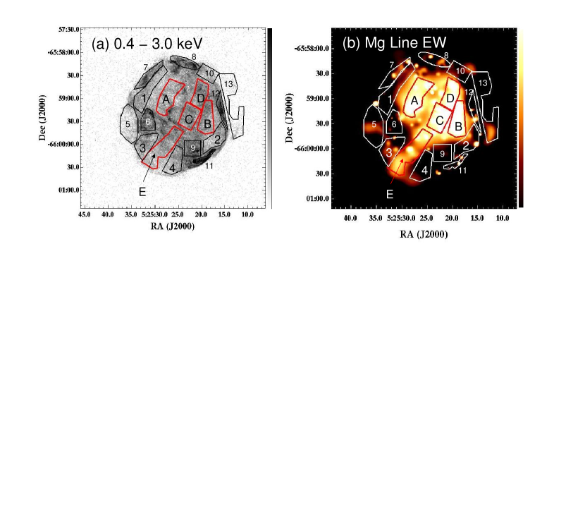
Figure 1.— (a) A broadband grey-scale Chandra ACIS image of N49B. The image has been binned by $\sim$1^′′ $\times$ 1^′′ pixels. (b) A false-color Mg line EW image of N49B. To create this map we used the ACIS subband images (see the text) with the original pixel size (0$.\mkern-4.0mu^{\prime\prime}$492), and adaptively smoothed them for the purposes of display. In (a) and (b), regions of our spectral analysis are overlaid.

Figure 2.— The ACIS spectrum extracted from region E (as marked in Figure 1). The best-fit two-component plane-shock model (solid curve) is overlaid. The soft (dotted) and hard (dashed) components of the best-fit plane shock model are overlaid. The bottom plot shows residuals from the best-fit model.

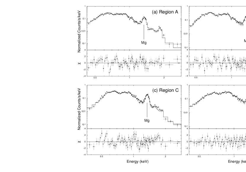
Figure 3.— The ACIS spectra extracted from Mg-overabundant regions (regions A, B, C, and D, as marked in Figure 1). The best-fit plane-shock model is overlaid in each panel. In each panel the bottom plot shows residuals from the best-fit model.

Figure 4.— Four example ACIS spectra extracted from shocked ISM regions (regions 1, 2, 3, and 4, as marked in Figure 1). The best-fit plane-shock model is overlaid in each panel. In each panel the bottom plot shows residuals from the best-fit model.

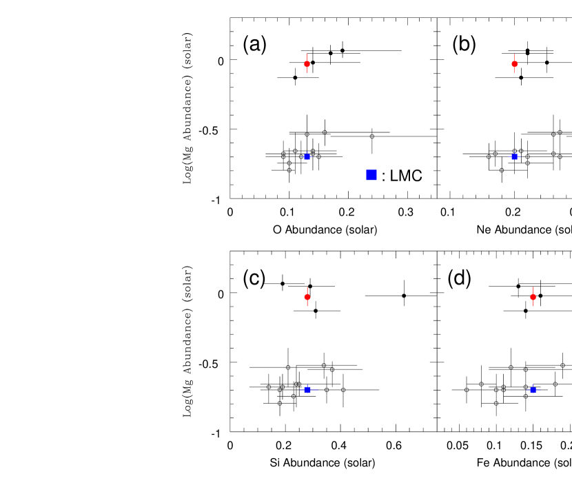
Figure 5.— Comparisons of Mg abundance with those of O, Ne, Si, and Fe for sub-regions of N49B. Black filled circles are regions A – D. The red filled circle shows the hard component of region E. Open circles are regions 1 – 12. The blue square is the LMC abundance (Schenck et al., 2016).

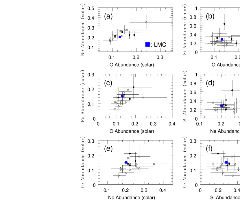
Figure 6.— Comparisons of measured elemental abundances (except for Mg) for sub-regions of N49B. Black filled circles are regions A – D, and open circles are regions 1 – 12. The blue square is the LMC abundance (Schenck et al., 2016). The LMC abundances are assumed for region E (see the text).

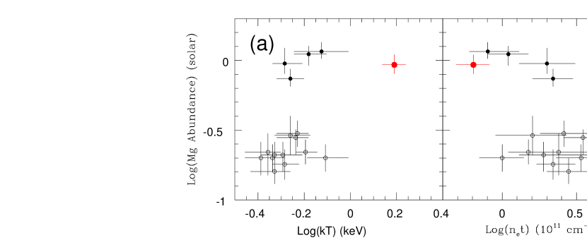
Figure 7.— Comparisons of Mg abundance with electron temperature and ionization timescale for sub-regions of N49B. Black filled circles are regions A – D. The red filled circle is the hard component of region E. Open circles are regions 1 – 12.

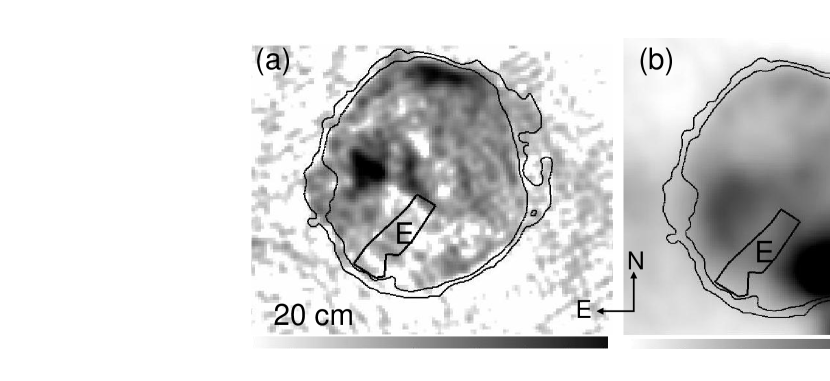
Figure 8.— (a) A grey-scale ATCA 20 cm image of N49B. The angular resolution (half-power beamwidth) is circular 6^′′. (b) A grey-scale 22 $\mu$m image of N49B from the public archive of the WISE all-sky survey data. The angular resolution is 12^′′. In (a) and (b) contours of the 0.3 – 3.0 keV ACIS image of N49B are overlaid to show the outer boundary of the SNR in the X-ray band. Region E is marked in (a) and (b).

References

- Anders & Grevesse (1989) Anders, E., & Grevesse, N. 1989, Geochimica et Cosmochimica Acta, 53, 197
- Badenes et al. (2006) Badenes, C., Borkowski, K. J., Hughes, J. P., Hwang, U., & Bravo, E. 2006, ApJ, 645, 1373
- Borkowski et al. (2001) Borkowski, K. J., Lyerly, W. J. & Reynolds, S. P. 2001, ApJ, 548, 820
- Chu & Kennicutt (1988) Chu, Y.-H, & Kennicutt, R. C. 1988, AJ, 96, 1874
- Cohen et al. (1988) Cohen, R. S., Dame, T. M., Garay, G., Montani, J., Rubio, M., & Thaddeus, P. 1988, ApJ, 331, L95
- Davies et al. (2015) Davies, B., Kudritzki, R.-P., Gazak, Z., Plez, B., Bergemann, M., Evans, C., & Patrick, L. 2015, ApJ, 806, 21
- Dickel & Milne (1998) Dickel, J. R., & Milne, D. K. 1998, AJ, 115, 1057
- Dickey & Lockman (1990) Dickey, J. M. & Lockman, F. J. 1990, ARA&A, 28, 215
- González-Casanova et al. (2014) González-Casanova, D. F., De Colle, F., Ramirez-Ruiz, E., & Lopez, L. A. 2014, ApJ, 781, L26
- Foster et al. (2012) Foster, A. R., Ji, L., Smith, R. K., & Brickhouse, N. 2012, ApJ, 756, 128
- Hester et al. (1994) Hester, J. J., Raymond, J. C., & Blair, W. P. 1994, ApJ, 420, 721
- Hughes et al. (1998) Hughes, J. P., Hayashi, I., & Koyama, K. 1998, ApJ, 505, 732
- Keohane et al. (2007) Keohane, J. W., Reach, W. T., Rho, J, & Jarrett, T. H. 2007, ApJ, 654, 938
- Lee et al. (2011) Lee, J.-J., Park, S., Hughes, J. P., Slane, P. O., & Burrows, D. N. 2011, ApJ, 731, L8
- Lopez et al. (2013) Lopez, L. A., Ramirez-Ruiz, E., Castro, D., & Pearson, S. 2013, ApJ, 764, 50
- Lopez et al. (2014) Lopez, L. A., Castro, D., Slane, P. O., Ramirez-Ruiz, E., & Badenes, C. 2014, ApJ, 788, 5
- Maggi et al. (2016) Maggi, P., Haberl, F., Kavanagh, P. J., Sasaki, M., Bozzetto, L. M., Filipovic,́ M. D., Vasilopoulos, G., Pietsch, W., Points, S. D., Chu, Y.-H., Dickel, J., Ehle, M., Williams, R., & Greiner, J. 2016, A&A, 585, 162
- Maeda & Nomoto (2003) Maeda, K. & Nomoto, K. 2003, ApJ, 598, 1163
- Meaburn et al. (1995) Meaburn, J., Bryce, M. & Holloway, A. J. 1995, A&A, 299, L1
- Nomoto et al. (2006) Nomoto, K., Tominaga, N., Umeda, H., Kobayashi, C., & Maeda, K. 2006, Nucl. Phys. A, 777, 424
- (21) Park, S., Burrows, D. N., Garmire, G. P., Nousek, J. A., Hughes, J. P., & Williams, R. M. 2003a, ApJ, 586, 210
- (22) Park, S., Hughes, J. P., Slane, P. O., Burrows, D. N., Warren, J. S., Garmire, G. P., & Nousek, J. A. 2003b, ApJ, 592, L41 (P03)
- Russell & Dopita (1992) Russell, S. C. & Dopita, M. A. 1992, ApJ, 384, 508
- Schenck et al. (2016) Schenck, A., Park, S., & Post, S. 2016, AJ, 151, 161
- Thielemann et al. (1996) Thielemann, F.-K., Nomoto, K., & Hashimoto, M.-A. 1996, ApJ, 460, 408
- Williams et al. (2006) Williams, B. J., Borkowski, K. J., Reynolds, S. P., Blair, W. P., Ghavamian, P., Hendrick, S. P., Long, K. S., Points, S., Raymonds, J. C., Sankrit, R., Smith, R. C., & Winkler, P. F. 2006, ApJ, 652, L33
- Williams et al. (2015) Williams, B. J., Rangelov, B., Kargaltsev, O., & Pavlov, G. G. 2015, ApJ, 808, L19