High-accuracy power series solutions with arbitrarily large radius of convergence for fractional nonlinear differential equations

Abstract

Fractional nonlinear differential equations present an interplay between two common and important effective descriptions used to simplify high dimensional or more complicated theories: nonlinearity and fractional derivatives. These effective descriptions thus appear commonly in physical and mathematical modeling. We present a new series method providing systematic controlled accuracy for solutions of fractional nonlinear differential equations. The method relies on spatially iterative use of power series expansions. Our approach permits an arbitrarily large radius of convergence and thus solves the typical divergence problem endemic to power series approaches. We apply our method to the fractional nonlinear Schrödinger equation and its imaginary time rotation, the fractional nonlinear diffusion equation. For the fractional nonlinear Schrödinger equation we find fractional generalizations of cnoidal waves of Jacobi elliptic functions as well as a fractional bright soliton. For the fractional nonlinear diffusion equation we find the combination of fractional and nonlinear effects results in a more strongly localized solution which nevertheless still exhibits power law tails, albeit at a much lower density.

I Introduction

Complexity is identified by a set of typical features complexityNAS2009 , ranging from complex network descriptions Newman2003 to chaos on strange attractors. Fractional descriptions lay at the foundation of many such features. For instance, strange attractors typically have fractional dimension. Complex networks exhibit log-normal or power-law statistics also associated with fractional derivatives West2014 . Fractional dimension is common in biological systems, e.g. the folds of the brain, the space-filling curve of DNA, and the maximization of surface area for gas exchange in the lungs and the branches of trees. Although foundational descriptions of physical phenomena typically take the form of partial differential equations (PDEs) or ordinary differential equations (ODEs) with derivatives of integer order, for example the diffusion equation, the wave equation, and the Schrödinger equation, it has been argued that effective PDE-based descriptions of complex phenomena require fractional partial derivatives West2014 ; he1 ; mai ; young . Indeed, the generalization of the diffusion equation to fractional derivatives has been found highly effective in describing for instance the propagation of ground water through soil benson2000 , the latter typically exhibiting multiscale properties. To what extent are fractional descriptions relevant to wave phenomena in general?

One natural context in which to examine this question is the nonlinear Schrödinger equation (NLSE). The NLSE appears in many contexts including the experimentally and theoretically well-established semiclassical effective limit of the quantum many-body description of Bose-Einstein condensates kevrekidisPG2008 ; the slowly varying envelope approximation for propagation of light in fiber optics Agrawal2001 ; and similar effective descriptions found for spin waves in ferromagnetic films kalinikos2000 . In every case the NLSE is an effective description, that is, starting from a much more complete but difficult to solve theory, one obtains a single scalar PDE/ODE that covers much of the observable phenomena in that system. An outstanding physical question is then the following. On the one hand fractional differential equations provide an effective description for complex multiscale phenomena in many contexts. On the other hand nonlinear PDEs/ODEs such as the NLSE are a highly useful simplification to reduce high dimensional or otherwise difficult problems to effective nonlinear differential equations. What is the interplay between these two key classes of effective PDE/ODE descriptions of complex systems?

The fractional generalization of the NLSE in particular has several useful limits in which the concept of effective theories can be carefully and rigorously explored. First, the linear limit of the Schrödinger equation is of course a well-understood problem. Second, the fractional generalization of the Schrödinger equation has been previously explored in many contexts laskin2002 ; ZhangAndBellic2016 . Third, the NLSE is an integrable equation with detailed solutions in terms of solitons. Fourth, by performing an imaginary time rotation the Schrödinger equation can be transformed to the diffusion equation. Fifth, the fractional diffusion equation, perhaps even more than the fractional Schrödinger equation, is a well-studied example with many special cases to draw on. Thus the fractional NLSE provides an ideal mathematical context in which to explore the interplay of nonlinearity and fractional derivatives in differential equations.

The basic concept of the fractional derivative is as old as calculus itself, originating in a discussion between L’Hôpital and Leibniz. In common usage now there are several approaches to fractionalize the derivative and several types of fractional derivatives have subsequently been introduced. The most popular ones are the Riemann-Liouville and Caputo fractional derivatives. The two definitions differ only in the order of evaluation. In the Caputo definition, we first compute an ordinary derivative then a fractional integral, while in the Riemann-Liouville definition the operators are reversed. It is often useful to apply the Caputo derivative in modeling, as mathematical modeling of many physical problems requires initial and boundary conditions, and these demands are satisfied using the Caputo fractional derivative. As fractional differential equations (FDEs) don’t generally possess exact closed form solutions, several analytical and numerical techniques have been implemented to study these equations. The series solution is one of the common techniques in studying FDEs analytically and numerically. For instance, the variational iteration method (VIM) Minc ; obidat1 , the homotopy analysis method (HAM) Song ; Sweilam , and the Adomian decomposition method (ADM) Gejji ; Jafari , have been implemented to study several types of FDEs. For more details one can refer to 100 and references therein. Recently, an efficient series solution was introduced for a class of nonlinear fractional differential equations alrefai1 . The idea is inspired by the Taylor series expansion method but it overcomes the difficulty of computing iterated fractional derivatives.

Despite these advances, there is no universal agreement on a series approach that unifies solutions to fractional, nonlinear, and fractional nonlinear differential equations. In this paper, we provide such an approach. Moreover, previous power series methods suffer from divergence past a finite radius of convergence. For example, if one considers the power series expansion of the bright soliton sech solution to the focusing NLSE, the radius of convergence is $\pi/2$. By extending the power series concept in a spatially iterative approach, we are able to move the radius of convergence to arbitrarily large values. To see why this is so important physically, consider the central limit theorem, which underpins statistical mechanics and indeed much of physical measurement in terms of the normal distribution. The central limit theorem only holds for finite variance. A well-known feature of the fractional diffusion equation is the power law tails of its localized solutions, which subsequently exhibit divergent variance. Such “fat-tailed” distributions lead to not-so-rare rare events and have practical outcomes such as the choice of whether or not to store radioactive waste a given distance from a population center Benson2006 . Our method allows us to benefit from the high accuracy and analytical formulation of the power series approach while not being subject to its typical problem with a physically limiting radius of convergence. We are able to extend the radius of convergence arbitrarily far into the tails of a localized solution, resulting in a clearer picture of the kind of statistics we can expect from the hybridization of nonlinear and fractional simplifications to physical problems.

II New power series ansatz

The common approach to the power series problem for fractional differential equations is an expansion of form

$$u(x)=\sum_{i=0}^{\infty}{a_{i}(x-x_{0})^{i\alpha}}.$$ (II.1)

This approach works well for linear fractional equations. However, for nonlinear fractional equations Eq. (II.1) has difficulties. Instead, we propose the following fractional power series as a solution:

$$u(x)=\sum_{i=0}^{n-1}{b_{i}(x-x_{0})^{i}}+\sum_{i=0}^{\infty}{a_{i}(x-x_{0})^{\alpha+i/q}},$$ (II.2)

where $n=[\alpha]$ denotes the nearest integer larger than $\alpha$ and $x_{0}$ is the value about which the expansion is performed. In comparison with the traditional expansion in powers of $i\alpha$ of Eq. (II.1), our proposal in the second term of Eq. (II.2), $\alpha+i/q$, is more comprehensive in the sense that the former is a subset of the latter. For instance, with $\alpha=3/2$ and $q=2$, the term $x^{5/2}$ will not be present in a power series of $x^{i\alpha}$, while in our case this will be included. In addition, such terms couple to the integer power terms in the first sum of Eq. (II.2) and to the nonlinear term leading to nontrivial recursion relations. It is essential for the method developed here that we have the integer power terms in the first sum of Eq. (II.2), which renders the current proposed fractional power series to be a necessity rather than a choice. Furthermore, when $q$ is even, our proposed power series will be valid also for the negative spatial domain.

In order to most effectively match the form of Eq. (II.2), we take the specific case of $\alpha=p/q$, where $p$ and $q$ are positive integers. Adopting here the Caputo sense cap for the fractional derivative, defined by

$$\frac{d^{\alpha}}{dx^{\alpha}}=\left\{\begin{array}[]{cc}\frac{1}{\Gamma(n-\alpha)}\int_{x_{0}}^{x}\frac{f^{(n)}(x^{\prime})}{(x-x^{\prime})^{\alpha-n}}\,dx^{\prime},&n-1<\alpha<n\,,\\ \\ \frac{d^{n}}{dx^{n}}f(x),&\alpha=n\,,\end{array}\right.$$ (II.3)

where $\Gamma(\cdot)$ is the well-known Gamma function, $f^{(n)}$ is the $n^{\mathrm{th}}$ order derivative of $f$, $x>x_{0}$, and $x_{0}$ is a constant which in our case will turn out to be the left side of the interval of spatial iteration in which we perform our power series expansion. For a power law, $f(x)=x^{k}$, where $k$ is an integer, the Caputo fractional derivative reduces to

$$\frac{d^{\alpha}}{dx^{\alpha}}x^{k}=\left\{\begin{array}[]{cc}\frac{\Gamma(k+1)}{\Gamma(k+1-\alpha)}x^{k-\alpha},&k\geq\alpha\,,\\ \\ 0,&k<\alpha\,.\end{array}\right.$$ (II.4)

For a shifted power law, $f(x)=(x-x_{0})^{k}$, where $x_{0}$ is real, the above expression is not applicable, as it would be in the case of regular derivatives: the chain rule for fractional derivatives takes a different form than an in the integer case. To resolve this matter we resort to the definition in Eq. (II.3) to obtain

$$\frac{d^{\alpha}}{dx^{\alpha}}\left(x-x_{0}\right)^{k}=$$ (II.5)

$$\left\{\begin{array}[]{cc}\frac{(k-1)k}{\Gamma(2-\alpha)}\left[\frac{\left(-x_{0}\right){}^{k}x^{1-\alpha}\left(-(\alpha-1)\,_{2}F_{1}\left(1,k-\alpha;k;\frac{x_{0}}{x_{0}-x}\right)+k-1\right)}{(k-1)x_{0}(k-\alpha)}-\frac{\pi\csc(\pi\alpha)\left(x-x_{0}\right){}^{k}\Gamma(k-1)\left(\frac{1}{x-x_{0}}\right){}^{\alpha}}{\Gamma(\alpha-1)\Gamma(k-\alpha+1)}\right],&1<\alpha<2\,,\\ \\ k(k-1)(x-x_{0})^{k-2},&\alpha=2\,,\end{array}\right.$$ (II.8)

where ${}_{2}F_{1}(\cdot)$ is the hypergeometric function and for simplicity we have written out explicitly the solution of the integral to the case $1<\alpha\leq 2$; solutions for other values of $\alpha$ can be obtained in the same manner. For physical applications $1<\alpha\leq 2$ is especially interesting as it interpolates between linear and quadratic disperson, i.e., between a phonon and a free particle. Bogoliubov theory also accomplishes such an interpolation fetterAL2001 but fractional derivatives are much more generic, e.g. in terms of capturing transport in a variety of multiscale media. Also, the nonlinear Dirac equation, obtained for example by optical means or a BEC in a honeycomb lattice carr2009g near the K-point, has a first order spatial derivative and linear dispersion. It should be noted here that Eq. (II.8) is applicable for $k\geq\alpha$. For $k<\alpha$, the fractional derivative equals zero for the case of integer $k$. This is so, since for integer $k$, the expression $(x-x_{0})^{k}$ can be expanded in powers of $x$ that are all less than $\alpha$, which, according to Eq. (II.4) will have zero fractional derivative.

For our iterative method it will turn out to be useful to consider the special cases of $k=\alpha$ and $k=\alpha+1$ with the result of the fractional derivative expanded around $x\to x_{0}^{+}$:

$$\frac{d^{\alpha}}{dx^{\alpha}}\left(x-x_{0}\right)^{\alpha}=\left\{\begin{array}[]{cc}c_{0}+c_{1}\log\left(\frac{x-x_{0}}{x_{0}}\right)+\mathcal{O}(x-x_{0}),&x_{0}>0\,,\\ \\ c_{0},&x_{0}=0\,,\end{array}\right.$$ (II.9)

$$c_{0} = -\frac{\pi(\alpha-1)\alpha\csc(\pi\alpha)}{\Gamma(2-\alpha)}+c_{1}\left(-\frac{1}{\alpha-1}+\psi^{(0)}(\alpha)+\gamma\right),$$

$$c_{1} = \frac{(-1)^{\alpha+1}(\alpha-1)\alpha}{\Gamma(2-\alpha)}\,,$$ (II.10)

where $\gamma$ is the Euler constant and $\psi^{(0)}(\alpha)$ is the digamma function defined by $\psi^{(0)}(z)=d\,{\rm Log}[\Gamma(z)]/dz$. For $x_{0}=0$ the $\alpha^{\rm th}$ derivative given by Eq. (II.9) is identical with that of Eq. (II.4) for $k=\alpha$, as it should be. For the case of $k=\alpha+1$:

$$\frac{d^{\alpha}}{dx^{\alpha}}\left(x-x_{0}\right)^{\alpha+1}=\left\{\begin{array}[]{cc}d_{0}+\left(d_{1}+d_{2}\log\left(\frac{x-x_{0}}{x_{0}}\right)\right)\left(x-x_{0}\right)+O[(x-x_{0})]^{2},&x_{0}>0\,,\\ \\ d_{3}x,&x_{0}=0\,,\end{array}\right.$$ (II.11)

where

$$d_{0} = \frac{(-1)^{\alpha+1}\alpha(\alpha+1)x_{0}}{\Gamma(2-\alpha)},$$

$$d_{1} = d_{2}\left(\psi^{(0)}(\alpha)+\gamma-1\right)+d_{3},$$

$$d_{2} = \frac{\alpha\left(\alpha^{2}-1\right)(-1)^{\alpha+1}}{\Gamma(2-\alpha)},$$

$$d_{3} = d_{2}(-1)^{-(\alpha+1)}\pi\csc(\pi\alpha)\,.$$ (II.12)

We note that the expansion of Eq. (II.9) diverges as $x\to x_{0}^{+}$ whereas Eq. (II.11) approaches a constant. This important observation will be exploited in the construction of the power series that is differentiable at $x_{0}$.

III Iterative solution method for the fractional nonlinear Schrödinger equation

We consider the following dimensionless fractional nonlinear Schr$\rm\ddot{o}$dinger equation (FNLSE)

$$i\frac{\partial}{\partial t}U(x,t)=-\frac{1}{2}\,\frac{\partial^{\alpha}}{\partial x^{\alpha}}U(x,t)-\gamma\,|U(x,t)|^{2}U(x,t)\,,$$ (III.1)

where $\gamma$ is the strength of the nonlinearity. The profile of the stationary solutions, $u(x)$, defined via $U(x,t)=u(x)\,\exp{(i\lambda\,t)}$, obeys the time-independent FNLDE

$${1\over 2}u-\frac{1}{2}\,\frac{d^{\alpha}}{dx^{\alpha}}u-\,u^{3}=0,$$ (III.2)

where we take $\lambda=1/2$ and $\gamma=1$ here and throughout such that for $\alpha=2$ the fundamental soliton $u(x)={\rm sech{({\it x}})}$ is an exact solution of Eq. (III.2). We note that due to the nonlinear nature of Eq. (III.2) the factor of $\gamma$ can be absorbed into the normalization without loss of generality, up to a sign: here we treat the focusing case. Likewise, taking $\lambda=1/2$ incurs no loss of generality, as it is simply a choice of units of time.

As a result of Eq. (II.4), the $\alpha^{\rm th}$-derivative of the first summation in Eq. (II.2) always vanishes. Therefore, the $b_{i}$ terms do not couple to terms of lower powers and thus correspond to the initial conditions such that for $0<\alpha\leq 1$ there is one initial condition, for $1<\alpha\leq 2$ there are two initial conditions, etc. Substituting the power series solution, Eq. (II.2) with $x_{0}=0$, in a nonlinear equation such as the FNLSE and using the Caputo fractional derivative, Eq. (II.4), it is straightforward to derive the recursion relations for $a_{i}$ in terms of the initial conditions $b_{i}$. However, the resulting power series solution suffers from the typical problem of finite radius of convergence which depends on $\alpha$ and equals $\pi/2$ for $\alpha=2$, as shown in Fig. 1.

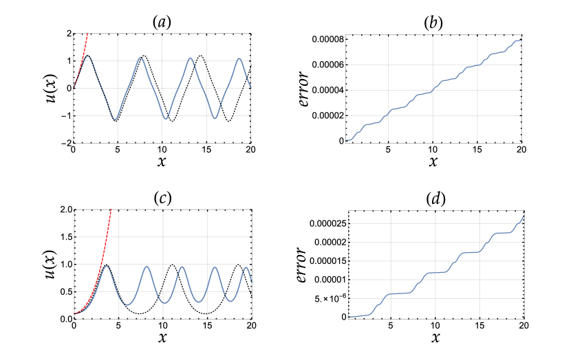
Figure 1: Iterative power series solutions of the fractional nonlinear Schrödinger equation. (Left column) Fractional generalizations of the well-known cnoidal wave solutions of the NLSE for $\alpha=4/3$: (a) Jacobi elliptic cn-like with nodes; (c) dn-like without nodes. Converged iterative fractional nonlinear power series solution introduced for the first time in this paper (blue curves) is compared to the rapid divergence of the usual fractional power series (red dashed curves). The well-known exact solutions for the NLSE are shown for comparison (black dotted curves). (Right column) (b), (d): Error incurred by our power series approach in each case increases arithmetically but remains below the predicted upper bound. The initial conditions are: $(u(0),u^{\prime}(0))=(0.0,0.8)$ and $(0.1,0.01)$ for (a) and (c), respectively. The number of iterations used is $N=10^{4}$.

To overcome this divergence problem, we implement the following iterative procedure. First, we divide $x$ into $N$ segments, each of width $\Delta=x/N$. Then we expand the solution starting with initial condition $x_{0}=0$, as given by Eq. (II.2). The resulting power series is then calculated at $x=\Delta$; providing the initial conditions for the next expansion around $x_{0}=\Delta$, and so on. However, two important issues need to be addressed before obtaining a well-behaved and convergent iterative power series solution using such an approach. The first is related to the logarithmic divergence of the $\alpha^{\rm th}$ derivative of $(x-x_{0})^{\alpha}$, as shown in Eqs. (II.9)-(II.11). The second is related to the convergence of the powers series in the number of iterations, that is, how does the result depend on the number of grid points $N$ and choice of interval $\Delta$?

An immediate problem arises in this procedure: the $\alpha^{\rm th}$ derivative of the term $(x-x_{0})^{\alpha}$ diverges logarithmically for $x_{0}\neq 0$, as shown in Eq. (II.9). Fortunately, from Eq. (II.11) we observe that the $\alpha^{\rm th}$ derivative of the term $(x-x_{0})^{\alpha+1}$ does not suffer from such a divergence. The best approach is thus to expand $u(x)$ as follows:

$$u(x)=\left\{\begin{array}[]{ll}b_{0}+b_{1}x+a_{1}x^{\alpha},&x_{0}=0\,,\\ \\ b_{0}+b_{1}(x-x_{0})+a_{1}(x-x_{0})^{\alpha+1},&x_{0}\neq 0\,.\end{array}\right.$$ (III.3)

In this manner, one avoids the logarithmic divergence. Substituting this expansion in Eq. (III.2), the recursion relation is obtained as

$$a_{1}=\left\{\begin{array}[]{ll}\frac{\Gamma(1)}{\Gamma(\alpha+1)}(b_{0}-2b_{0}^{3}),&x_{0}=0\,,\\ \\ \frac{\Gamma(2-\alpha)}{(-1)^{1+\alpha}\alpha(\alpha+1)x_{0}}(b_{0}-2b_{0}^{3}),&x_{0}\neq 0\,.\end{array}\right.$$ (III.4)

Then we calculate the series, Eq. (III.3) for $x_{0}=0$, at $x=\Delta$, from which we calculate the new initial conditions

$$b_{0} \leftarrow u(\Delta)=b_{0}+b_{1}\Delta+a_{1}\Delta^{\alpha}\,,$$ (III.5)

$$b_{1} \leftarrow u^{\prime}(\Delta)=b_{1}+\alpha a_{1}\Delta^{\alpha-1}.$$ (III.6)

The new values of $b_{0}$ and $b_{1}$ are then substituted back in Eq. (III.3), for $x_{0}=\Delta$, which in turn is then substituted in Eq. (III.2) to give the new recursion relation. It should be noted here that due to the homogeneity of the differential equation at hand, Eq. (III.2), the recursion relation $a_{1}(a_{0})$ is essentially the same for all iterations, as given by Eq. (III.3) for $x_{0}\neq 0$. This procedure is repeated $N$ times, leading to a power series free from the intrinsic divergence problem in the original series. In the case of inhomogeneous differential equations, where the coefficients of $u$ and its derivatives are functions of $x$, the recursion relation $a_{1}(a_{0})$ will be different for each iteration and has to be calculated at every iteration step.

However, the iterative procedure turns out to suffer from another serious problem. The solutions do not converge when $N\rightarrow\infty$. In a well-behaved iteration method, the solution should converge to a certain profile when $N$ is sufficiently increased. Careful investigation shows that this problem stems from the fact that the higher derivatives of the iterated power series are not continuous at the boundaries between the $i\Delta$ and $(i+1)\Delta$ expansions. Basically, it is the iterative procedure itself that causes this problem. When we calculate the series $u(i\Delta)$ and its derivative $u^{\prime}(i\Delta)$ and pass these values to the $b_{0}$ and $b_{1}$ of the new series, we guarantee the continuity in the solution and its derivative only. The second derivative and higher derivatives are not continuous due to the fractional powers. This problem is absent in the case of integer power series but is an intrinsic problem in series with fractional powers. In the following we present a remedy to this difficulty.

Consider series zeroth-order series

$$u_{0}(x)=b_{0}+b_{1}x+a_{1}x^{\alpha}.$$ (III.7)

Substituting $b_{0}=u_{0}(\Delta)$ and $b_{1}=u_{0}^{\prime}(\Delta)$, we obtain the first iterated series

$$u_{1}(x)=b_{0}+2b_{1}x+(\alpha+2)a_{1}x^{\alpha}.$$ (III.8)

For the iterated series to be convergent with the number of iterations, $N$, it must be equal to the non-iterated series calculated at $N\Delta$, namely

$$u_{N}(\Delta)=u_{0}(N\Delta).$$ (III.9)

Applying this condition for $N=1$,

$$b_{0}+b_{1}(2\Delta)+a_{1}(2\Delta)^{\alpha}=b_{0}+2b_{1}\Delta+(\alpha+2)a_{1}\Delta^{\alpha}.$$ (III.10)

The zeroth- and first-order terms clearly satisfy this condition, but the $\alpha^{\rm th}$-term acquires an additional factor of $(\alpha+2)$. This requires the replacement $a_{1}\rightarrow a_{1}\times 2^{\alpha}/(\alpha+2)$ in the right hand side of this equation. Here we show the result of the next few iterations:

$$u_{2}(x) = b_{0}+3b_{1}x+(3\alpha+3)a_{1}x^{\alpha},$$

$$u_{3}(x) = b_{0}+4b_{1}x+(6\alpha+4)a_{1}x^{\alpha},$$

$$u_{4}(x) = b_{0}+5b_{1}x+(10\alpha+5)a_{1}x^{\alpha},$$

$$u_{5}(x) = b_{0}+6b_{1}x+(15\alpha+6)a_{1}x^{\alpha},$$

$$\dots$$

$$u_{N-1}(x) = b_{0}+N\,b_{1}x+[N+1+\frac{1}{2}N(N+1)\alpha]a_{1}x^{\alpha},$$ (III.11)

where the closed form for the general term was found by inspection. Applying the condition (III.9) requires

$$a_{1}\rightarrow a_{1}\times\frac{N^{\alpha}}{N+1+\frac{1}{2}N(N+1)\alpha}\,.$$ (III.12)

This condition is required to be satisfied in the limit of large $N$, which then takes the form

$$a_{1}\rightarrow a_{1}\times\frac{2}{\alpha}N^{\alpha-2}\,.$$ (III.13)

It should be noted that applying any of the last two conditions to the series given by Eq. (III.3) for $x_{0}\neq 0$ requires replacing $\alpha$ by $\alpha+1$ in the last two equations. In addition, Eqs. (III.3) and (III.4) show that $u(x)$ depends on $x_{0}$ also through $a_{1}\propto 1/x_{0}$. Taking this into account and repeating the iterative procedure described above but now with $u(x)=b_{0}+b_{1}(x-x_{0})+a_{1}(x-x_{0})^{\alpha+1}$, which is the second line of Eq. (III.3), we obtain finally the correction replacement rule:

$$a_{1}\rightarrow a_{1}\times(-1)^{\alpha+1}\Delta\frac{N^{\alpha+1}}{N+1+\frac{1}{2}N(N+1)(\alpha+1)}\,.$$ (III.14)

The appearance of the factor $(-1)^{\alpha+1}$ suggests specific fractional values of $\alpha=p/q$ with $q$ being an odd integer. Otherwise, $a_{1}$ will become complex.

The resulting series for the FNLSE corresponds to a host of oscillatory and localized solutions characterized by values of $b_{0}$ and $b_{1}$. The initial slope of the solution, $b_{1}$, will not have a significant effect on the nature of the solutions other than an overall shift along the $x$-axis. Inspection shows that generally the solutions are oscillatory apart from localized solutions obtained with some specific values of $b_{0}$.

III.1 Fractional Cnoidal Waves

In Fig. 1, we plot two fundamental solutions of the FNLSE using this iterative procedure. As clearly shown in this figure, the power series solution without using the iterative procedure, (II.2), diverges at $x\sim\pi/2$, but after applying our iterative method the divergence is removed. Indeed, implementing the correction procedure solves also the problem of lack of convergence; the solutions are stable beyond a number of iterations greater than about 2000. Another criterion that our solutions should satisfy is that they must match the non-iterated series for a range less than the radius of convergence, which is indeed the case, as Fig. 1 also shows. In Fig. 2, we show a localized solution for different values of $\alpha$ with $b_{0}$ tuned up to a certain precision in order to push oscillations away from the origin to a certain distance. The analogous localized solution for the $\alpha=2$ case is the fundamental soliton given by $u(x)={\rm sech}(x)$, which is also plotted in Fig. 2.

Error in the iterative series solution persists due to terminating the power series at a finite number of terms, say $k$. It is instructive at this point to estimate the magnitude of this error. Terminating the second summation in Eq. (II.2) at $i=k$ results in an error of order $\Delta^{\alpha+(k+1)/q}$. This error will be magnified $N$ times due to the iterative procedure. Therefore, the estimated error in our method is of order

$${\rm error_{max}}\propto N\left(\frac{x}{N}\right)^{\alpha+(k+1)/q}=N^{1-\alpha-(k+1)/q}\,x^{\alpha+(k+1)/q}.$$ (III.15)

This estimate can be taken as an upper bound on the actual error, which we define as

$${\rm error}=\frac{1}{x}\int_{0}^{x}\left|\frac{1}{2}u(x^{\prime})-\frac{1}{2}\frac{d^{\alpha}}{dx^{\prime\alpha}}u(x^{\prime})-u(x^{\prime})^{3}\right|^{2}\,dx^{\prime},$$ (III.16)

where $u(x^{\prime})$ is the solution found by the iterative power series. In the right column of Fig. (1), we plot this error as a function of $x$. We find the error increases linearly with $x$ but remains below the upper bound (III.15) for the parameters used.

III.2 Fractional Solitons

In Fig. 2(a) we explore localized solutions more closely, where we show their dependence on $\alpha$ as well as the structure of the tail. We may loosely call this solution the fractional soliton, recognizing that for now we have not shown stability. We note that as $\alpha$ decreases the soliton becomes narrower, i.e., is more strongly localized. This can be understood based on the balance between nonlinearity and dispersion that supports a soliton. Decreasing $\alpha$ effectively decreases the strength of the dispersion, and as the nonlinearity is of focusing type, the soliton becomes narrower. However, we point out that this trend is opposite to that predicted by the usual scaling argument based on a variational calculation of the total energy. The scaling behavior of Eq. (III.2) obtained in such a manner would naively be $f\propto 1/\ell^{\alpha}-1/\ell$, with $\ell$ an estimate of the width of the fractional soliton, as follows also from the $1/\sqrt{\ell}$ units of $u(x)$. However, solving for $df/d\ell=0$ results in $\ell_{\mathrm{min}}=\alpha^{1/(\alpha-1)}$, predicting a decreasing width for increasing $\alpha$, clearly in contradiction to the more accurate power series approach. In the future it would be useful to develop a proper variational analysis via a Lagrangian variational dynamical approach perez1997 to obtain a more precise estimate of fractional soliton widths and breathing frequencies. This requires rethinking the energy contribution of the fractional derivative.

As illustrated in Fig. 2(b) our iterative power series approach finds that the tail is exponential in nature, in contrast to the well-known power-law behavior for the fractional diffusion equation discussed in Sec. IV. Although it would seem the tail of a localized solution of any nonlinear fractional equation should approach the tail of the corresponding linear fractional equation, this is not at all obvious since a tail grows rapidly flat, and one must closely examine the balance between shrinking nonlinearity and decreasing derivative on the tail. We find the prefactor in the exponential decreases monotonically with $\alpha$.

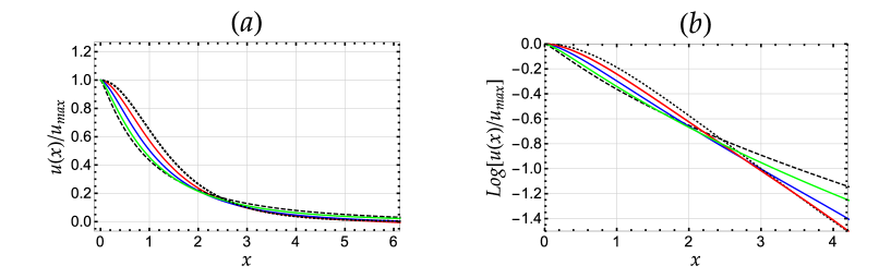
Figure 2: Fractional generalization of the bright soliton. (a) Localized solution obtained via nonlinear fractional power series for values of $\alpha$ ranging between linear (dashed curve) and quadratic (dotted curve) dispersion: $\alpha=1.0001,18/15,22/15,26/15,2$. The usual $\alpha=2$ bright soliton, shown for comparison, is identical with ${\rm sech}(x)$. Note that, for comparative purposes only, we renormalize the fractional soliton to its maximal value, plotting $u(x)/u_{\mathrm{max}}$ vs. $x$. (b) The tails of such solutions remain exponentially decreasing and are therefore of finite variance.

IV Application to the fractional nonlinear diffusion equation

It is well known that the imaginary time rotation of the Schrödinger equation $\tau=-it$ produces the diffusion equation. Both nonlinear and fractional extensions of these equations are connected in the same way, and thus the case study for our power series in Sec. III is easily applied to the fractional nonlinear diffusion equation. This is an especially interesting case because the fractional diffusion equation has well-known power law tails exhibiting a divergent variance.

The fractional diffusion equation takes the form

$$\frac{\partial u(x,\tau)}{\partial\tau}=\frac{\partial^{\alpha}u(x,\tau)}{\partial x^{\alpha}}\,.$$ (IV.1)

This well-studied equation is usually solved by the Fourier transform method. For $\alpha=2$ the solution is the Gaussian function

$$u(x,\tau)=\frac{c}{\sqrt{\tau}}e^{-\frac{x^{2}}{4\tau}}\,,$$ (IV.2)

where $c$ is an arbitrary real constant. For the fractional case, the solution is still localized, but with an algebraically decaying tail of form $|x|^{-(\alpha+1)}$ benson2000 . This is a distinctive feature of the fractional diffusion equation which we aim at obtaining using the present method.

Based on the special case of $\alpha=2$, a simple scaling argument may be used to deduce that the solution scales as

$$u(x,\tau)=\frac{1}{\sqrt{\tau}}\,v\left(\frac{x}{2\sqrt{\tau}}\right)\,,$$ (IV.3)

which suggests the following series expansion:

$$u(x,\tau)=\frac{1}{\sqrt{\tau}}\left[b_{0}+b_{1}\left(\frac{x}{2\sqrt{\tau}}\right)+a_{1}\left(\frac{x}{2\sqrt{\tau}}\right)^{\alpha}\right].$$ (IV.4)

Applying the iterative power series method as described above, we obtain the desired results, as shown in Fig. 3. On a log-log scale, Fig. 3(b) shows clearly that the tail is decaying algebraically, as expected, with the correct exponent of the power law. Due to the fact that the diffusion equation is linear a rather small number of iterations, $N=30$, is enough to obtain solutions that converge against increasing the number of iterations. While the algebraic decay of the tail is accounted for qualitatively, a quantitative account requires a more rigorous treatment in which we do not use the above-mentioned specific scaling. This in turn requires a generalisation of the present method to partial differential equations, which we leave to future work.

Finally, we apply our method to the nonlinear fractional diffusion equation

$$\frac{\partial u(x,\tau)}{\partial\tau}=\frac{\partial^{\alpha}u(x,\tau)}{\partial x^{\alpha}}-\gamma u(x,\tau)^{3},$$ (IV.5)

where $\gamma$ is a positive constant. The effect of the cubic nonlinear term is shown in Fig. 4 where we compare with the linear case. The algebraic decay of the tail persists in the nonlinear case but at a much lower density than for the linear case. Thus the focusing nonlinearity localizes the solution much more strongly than in the linear case, but in the end the power law is the same, indicating that the fractional derivative dominates over the nonlinearity asymptotically just like in the integer derivative case.

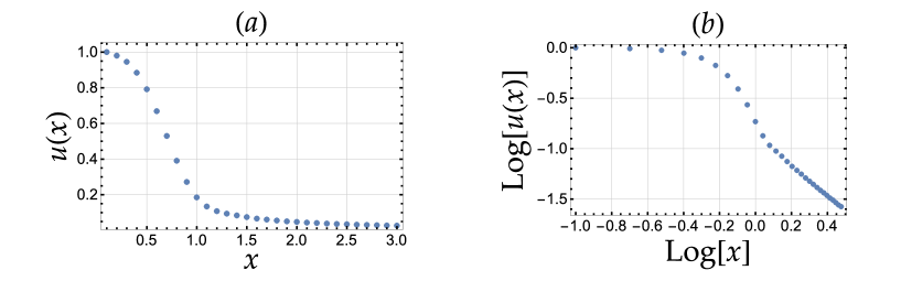
Figure 3: Power law tails in fractional diffusion equation. Solution of the fractional diffusion equation, Eq. (IV.1) at $\tau=1$ and for $\alpha=4/3$. We used the initial conditions $u(0)=1$ and $u^{\prime}(0)=0$. Number of iterations used is $N=30$.

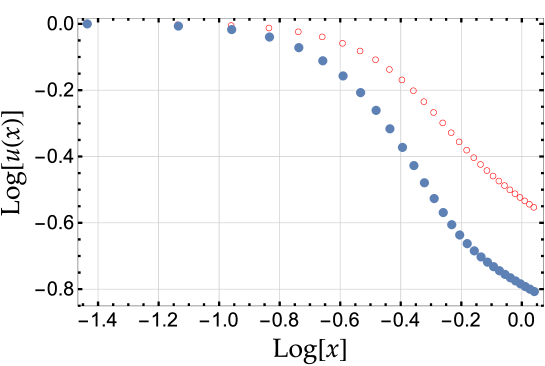
Figure 4: Localized solutions in the fractional nonlinear diffusion equation. Solution of the nonlinear fractional diffusion equation, Eq. (IV.5) at $\tau=1$, for $\alpha=4/3$, and $\gamma=1$ (Blue filled circles). Red empty circles correspond to the linear case, $\gamma=0$. We used the initial conditions $u(0)=1$ and $u^{\prime}(0)=0$. Number of iterations used is $N=2000$.

V Conclusions

We developed a new iterative power series approach to solve fractional nonlinear differential equations. The use of iteration allows one to overcome the usual radius of convergence problems associated with power series. We provided an explicit upper bound on the error of our method in the total number of spatial iterations and the grid size, or spatial interval. We applied our method to the fractional nonlinear Schrödinger equation (FNLSE) and its imaginary time rotation, the fractional nonlinear diffusion equation. We found fractional generalizations of cnoidal waves and introduced the fractional soliton for the focusing FNLSE. For the fractional nonlinear diffusion equation we showed power law tails persist, although at a much lower density than in the linear case: thus fractional dispersion dominates nonlinearity asymptotically. In future work the method can be applied to a wide variety of nonlinear fractional equations, the most obvious being the defocusing FNLSE case where one can study the properties of fractional dark solitons.

References

- (1) The National Academies Keck Futures Initiative: Complex Systems: Task Group Summaries. The National Academies Press, Washington, D.C., 2009.
- (2) M. E. J. Newman. The Structure and Function of Complex Networks. SIAM Review, 45:167–256, 2003.
- (3) Bruce J. West. Colloquium : Fractional calculus view of complexity: A tutorial. Rev. Mod. Phys., 86:1169–1186, 2014.
- (4) J. H. He. Some applications of nonlinear fractional differential equations and their approximations. Bull. Sci. Technol., 15:86, 1999.
- (5) F. Mainardi. Fractals and Fractional calculus in Continuum Mechanics, chapter Fractional calculus: Some basic problems in continum and statistical mechanics, pages 291–348. Springer-Verlag, New York, NY, 1997.
- (6) H. Beyer and S. Kempfle. Definition of physically consistent damping laws with fractional derivatives. ZAMM - Journal of Applied Mathematics and Mechanics / Zeitschrift für Angewandte Mathematik und Mechanik, 75:623–635, 1995.
- (7) D. A. Benson, S. W. Wheatcraft, and M. M. Meerschaert. Application of a fractional advection-dispersion equation. Water Resources Research, 36:1403, 2000.
- (8) P. G. Kevrekidis, D. J. Frantzeskakis, and R. Carretero-González, editors. Emergent Nonlinear Phenomena in Bose-Einstein Condensates. Springer-Verlag, Berlin, 2008.
- (9) G.P. Agrawal. Nonlinear Fiber Optics. Academic Press, New York, 2001.
- (10) B. A. Kalinikos, M. M. Scott, and C. E. Patton. Self-generation of fundamental dark solitons in magnetic films. Phys. Rev. Lett., 84:4697–4700, 2000.
- (11) Nick Laskin. Fractional schrödinger equation. Phys. Rev. E, 66:056108, 2002.
- (12) D. Zhang, Y. Zhang, Z. Zhang, N. Ahmed, Y. Zhang, F. Li, M. R. Belić, and M. Xiao. Unveiling the link between fractional Schr”odinger equation and light propagation in honeycomb lattice. ArXiv e-prints, 2016.
- (13) Mustafa Inc. The approximate and exact solutions of the space- and time-fractional burgers equations with initial conditions by variational iteration method. Journal of Mathematical Analysis and Applications, 345(1):476, 2008.
- (14) Zaid Odibat and Shaher Momani. The variational iteration method: An efficient scheme for handling fractional partial differential equations in fluid mechanics. Computers & Mathematics with Applications, 58:2199, 2009.
- (15) Lina Song and Hongqing Zhang. Application of homotopy analysis method to fractional kdv–burgers–kuramoto equation. Physics Letters A, 367:88, 2007.
- (16) N.H. Sweilam, M.M. Khader, and R.F. Al-Bar. Numerical studies for a multi-order fractional differential equation. Physics Letters A, 371:26, 2007.
- (17) Varsha Daftardar-Gejji and Sachin Bhalekar. Solving multi-term linear and non-linear diffusion–wave equations of fractional order by adomian decomposition method. Applied Mathematics and Computation, 202:113, 2008.
- (18) Hossein Jafari and Varsha Daftardar-Gejji. Solving linear and nonlinear fractional diffusion and wave equations by adomian decomposition. Applied Mathematics and Computation, 180:488, 2006.
- (19) Marc Weilbeer. Efficient numerical methods for fractional differential equations and their analytical background. PhD thesis, Technischen Universität Braunschweig, 2005.
- (20) M. Al-Refai, M. Hajji, and M. Syam. An efficient series solution for fractional differential equations. Abstract and Applied Analysis, 2014:891837, 2014.
- (21) David A. Benson, Mark M. Meerschaert, Boris Baeumer, and Hans-Peter Scheffler. Aquifer operator scaling and the effect on solute mixing and dispersion. Water Resources Research, 42:W01415, 2006.
- (22) Michele Caputo. Linear models of dissipation whose q is almost frequency independent—ii. Geophysical Journal International, 13:529, 1967.
- (23) A. L. Fetter and A. A. Svidzinsky. Vortices in a trapped dilute Bose-Einstein condensate. J. Phys.: Condens. Matter, 13:R135–R194, 2001.
- (24) L. H. Haddad and L. D. Carr. The nonlinear Dirac equation in Bose-Einstein condensates: Foundation and symmetries. Physica D: Nonlinear Phenomena, 238:1413, 2009.
- (25) V. M. Pérez-García, H. Michinel, J. I. Cirac, M. Lewenstein, and P. Zoller. Dynamics of Bose-Einstein condensates: variational solutions of the Gross-pitaevskii equations. Phys. Rev. A, 56:1424–1432, 1997.