Astrochemical Properties of Planck Cold Clumps

Abstract

We observed thirteen Planck cold clumps with the James Clerk Maxwell Telescope/SCUBA-2 and with the Nobeyama 45 m radio telescope. The N₂H⁺ distribution obtained with the Nobeyama telescope is quite similar to SCUBA-2 dust distribution. The 82 GHz HC₃N, 82 GHz CCS, and 94 GHz CCS emission are often distributed differently with respect to the N₂H⁺ emission. The CCS emission, which is known to be abundant in starless molecular cloud cores, is often very clumpy in the observed targets. We made deep single-pointing observations in DNC, HN¹³C, N₂D⁺, cyclic-C₃H₂ toward nine clumps. The detection rate of N₂D⁺ is 50%. Furthermore, we observed the NH₃ emission toward 15 Planck cold clumps to estimate the kinetic temperature, and confirmed that most of targets are cold ($\lesssim$ 20 K). In two of the starless clumps observe, the CCS emission is distributed as it surrounds the N₂H⁺ core (chemically evolved gas), which resembles the case of L1544, a prestellar core showing collapse. In addition, we detected both DNC and N₂D⁺. These two clumps are most likely on the verge of star formation. We introduce the Chemical Evolution Factor (CEF) for starless cores to describe the chemical evolutionary stage, and analyze the observed Planck cold clumps.

=1 The Friends of AASTeX Collaboration

1 Introduction

On the basis of the Planck all-sky survey (Planck Collaboration XXIII, 2011; Planck Collaboration XXVIII, 2016), we are carrying out a series of observations of molecular clouds as the Planck Cold Clump collaboration in order to understand the initial condition for star formation (Liu et al., 2015). Planck cold clumps have low dust temperatures (10$-$20 K; median=14.5 K). Pilot observations have been carried out with various ground-based telescopes such as JCMT, IRAM, PMO 14m, APEX, Mopra, Effelsberg, CSO, and SMA (Liu et al., 2015). A Large Program for JCMT dust continuum observations with SCUBA-2 (SCOPE : SCUBA-2 Continuum Observations of Pre-protostellar Evolution; Thompson et al. 2017, in preparation) and a Key Science Program with TRAO 14 m radio telescope (TOP : TRAO Observations of Planck cold clumps; Liu et al. 2017, in preparation) are ongoing.

To characterize Planck cold clumps, it is essential to investigate their chemical and physical properties in detail. In particular, we try to make their evolutionary stages clear. The chemical evolution of molecular clouds has been established to some extent, not only for nearby dark clouds (e.g., Suzuki et al. (1992); Hirahara et al. (1992); Benson, Caselli, & Myers (1998); Hirota & Yamamoto (2006); Hirota, Ohishi, & Yamamoto (2009), but also for giant molecular clouds (GMCs; Tatematsu et al. (2010, 2014a); Ohashi et al. (2014) for Orion A GMC; Ohashi et al. (2016a) for Vela C GMC; Sanhueza et al. (2012); Hoq et al. (2013) for Infrared Dark Clouds). Carbon-chain molecules such as CCS and HC₃N tend to be abundant in starless molecular cloud cores, while N-bearing molecules such as NH₃ and N₂H⁺ as well as c-C₃H₂ tend to be abundant in star-forming molecular cloud cores. However, N₂H⁺ will be destroyed by evaporated CO in warm cores having $T_{dust}\gtrsim$ 25 K (Lee et al., 2004), and therefore $N$(N₂H⁺)/$N$(CCS) may not be a good evolutionary tracer for $T_{dust}\gtrsim$ 25 K. In a survey of nearby cold dark cloud cores, Suzuki et al. (1992) detected CCS 45 GHz in 55% of the observed cores, and found that CCS is a tracer of the young molecular gas in starless cloud cores. Tatematsu et al. (2010) detected CCS$J_{N}$ = $4_{3}-3_{2}$ at 45 GHz in 32% of the cores observed toward Orion A GMC. Sakai et al. (2008) observed 55 massive clumps associated with Infrared Dark Clouds (IRDCs) in CCS $J_{N}$ = $4_{3}-3_{2}$ at 45 GHz using the Nobeyama 45 m telescope, and detected this line in none of them. Dirienzo et al (2015) observed nine IRDCs in CCS $J_{N}$ = $2_{1}-1_{0}$ at 24 GHz using VLA, and detected this line in all of them.

Furthermore, deuterium fractionation ratios are powerful evolutionary tracers (Hirota & Yamamoto, 2006; Sakai et al., 2012). The deuterium fraction D/H in molecules in molecular clouds is larger than the terrestrial abundance ratio (1.15$\times 10^{-4}$) or the protosolar estimate (2$\times 10^{-5}$) (Geiss & Reeves, 1981). The deuterium fraction is enhanced in molecular cloud cores before star formation (prestellar phase), which is cold enough, and the ratio increases with prestellar evolution until star formation (Crapsi et al., 2005; Hirota & Yamamoto, 2006). However, it should be noted that the deuterium fraction decreases with increasing temperature (Snell & Wootten, 1979; Wootten, 1987; Schilke et al., 1992; Tatematsu et al., 2010). After star formation, the deuterium fraction decreases (Emprechtinger et al., 2009). $N$(DNC)/$N$(HNC) will decrease, which may in part be due to an increase in the kinetic temperature, but may be affected by a larger reaction timescale (several times 10⁴ yr) while $N$(N₂D⁺)/$N$(N₂H⁺) will reflect the current temperature more directly, because of a shorter reaction time scale (less than 100 years) (Sakai et al., 2012).

We investigate the evolutionary stages of Planck cold clumps using molecular column density ratios. For this purpose, by using the Nobeyama 45 m telescope, we observed 13 Planck cold clumps, for which we have already obtained accurate positions from preliminary IRAM 30m observations in N₂H⁺ and/or SCUBA-2 observations. We selected sources whose C¹⁸O $J$ = 1$-$0 linewidths are relatively narrow ($<$ 1.5 km s^-1) from the previous observations with the 13.7 m telescope of the Purple Mountain Observatory (PMO) at De Ling Ha, because we prefer to observe relatively close objects to investigate the chemical differentiation on scales of 0.05-0.1 pc (Tatematsu et al., 2014a; Ohashi et al., 2014, 2016a). However, some of our sources (G108.8-00.8 and G120.7+2.7) are actually distant (1-3.5 kpc), which needs some care in discussion based on the column density ratios. While we focus on the chemical evolution stage as the main target of the current study, we also briefly investigate the physical properties of the sources by analyzing the specific angular momenta.

2 Observations

2.1 James Clerk Maxwell Telescope

Observations with the 15 m James Clerk Maxwell Telescope (JCMT) on Mauna Kea were made between 2014 November and 2015 December in the pilot survey phase (project IDs: M15AI05, M15BI061) of the JCMT legacy survey program “SCOPE”. The Submillimetre Common-User Bolometer Array 2 (SCUBA-2) was employed for observations of the 850 $\mu$m continuum. It is a 10,000 pixel bolometer camera operating simultaneously at 450 and 850 $\micron$. Observations were carried out in constant velocity (CV) Daisy mode under grade 3/4 weather conditions with a 225 GHz opacity between 0.1 and 0.15. The mapping area is about $12\arcmin\times$12′. The beam size of SCUBA-2 at 850 $\micron$ is $\sim$14$\arcsec$. The typical rms noise level of the maps is about 6-10 mJy beam^-1 in the central 3$\arcmin$ area, and increases to 10-30 mJy beam^-1 out to 12$\arcmin$. The data were reduced using SMURF in the STARLINK package.

2.2 Nobeyama 45 m Telescope

Observations with the 45 m radio telescope of Nobeyama Radio Observatory were carried out from 2015 December to 2016 February. We observed eight molecular lines by using the receivers TZ1 and T70 (Table 1). Observations with the receiver TZ1 (we used one beam called TZ1 out of two beams of the receiver TZ) (Asayama & Nakajima, 2013; Nakajima et al., 2013) were made to simultaneously observe four molecular lines, 82 GHz CCS, 94 GHz CCS, HC₃N and N₂H⁺. Observations were carried out with T70 to simultaneously observe four other lines, HN¹³C, DNC, N₂D⁺, and cyclic-C₃H₂. TZ1 and T70 are double-polarization, two-sideband SIS receivers. Molecular transitions are selected to achieve a high angular resolution of $\sim$20” to differentiate the distribution of molecules, and they are detectable even from cold gas ($\lesssim$ 20 K). The upper energy level $E_{u}$ of the observed transitions are listed in Table 1.

The FWHM beam sizes at 86 GHz with TZ1 and T70 were 18$\farcs$2$\pm$0$\farcs$1 and 18$\farcs$8$\pm$0$\farcs$3, respectively. The main-beam efficiency $\eta_{mb}$ at 86 GHz with TZ1 was 54$\pm$3% and 53$\pm$3% in H and V polarizations, respectively. The efficiencies with T70 was 54$\pm$3% and 55$\pm$3% in H and V polarizations, respectively. We also observed NH₃ $(J,K)$ = (1, 1) at 23.694495 GHz (Ho & Townes, 1983) in both circular polarizations with the receiver H22. The FWHM beam size at 23 GHz with H22 was 74$\farcs$4$\pm$0$\farcs$3 and 73$\farcs$9$\pm$0$\farcs$3 for ch1 and ch2 (right-handed and left-handed circular polarization), respectively. The main-beam efficiency $\eta_{mb}$ at 23 GHz with H22 was 83$\pm$4% and 84$\pm$4%, for ch1 and ch2, respectively. The receiver backend was the digital spectrometer “SAM45”. The spectral resolution was 15.26 kHz (corresponding to 0.05$-$0.06 km s^-1) for TZ1 and T70, and 3.81 kHz (corresponding to $\sim$0.05 km s^-1) for H22.

Observations with receiver TZ1 were conducted in the on-the-fly (OTF) mapping mode (Sawada et al., 2008) with data sampling intervals along a strip of 5$\arcsec$ and separations between strips of 5$\arcsec$. We have made orthogonal scans in RA and DEC to minimize scan effects. Observations with receivers T70 and H22 were carried out in the ON-OFF position-switching mode. The ON positions with receiver T70 were determined from possible intensity peaks in N₂H⁺ on temporal lower-S/N-ratio TZ1 maps during observations (before completion), but are not necessarily intensity peaks in N₂H⁺ on the final maps. In addition, the T70 position of G207N was incorrect.

Coordinates used for the observations are listed in Table 2. The distances to the sources are taken from Ramirez Alegria et al. (2011) for G108.8-00.8, Wu (2012) for G120.7+2.7, Lombardi et al. (2010) for G157.6-12.2, Loinard et al. (2007) and Lombardi et al. (2010) for G174.0-15.8, Kim et al. (2008) for G192.33-11.88, G202.31-8.92, G204.4-11.3, and G207.3-19.8, and Clariá (1974) for G224.4-0.6. Those to G089.9-01.9, G149.5-1.2, and G202.00+2.65 are taken from Planck Collaboration XXVIII (2016).

The observed intensity is reported in terms of the corrected antenna temperature $T_{A}^{*}$. To derive the physical parameters, we use the main-beam radiation temperature $T_{mb}$ = $T_{A}^{*}$/$\eta_{mb}$. The telescope pointing was established by observing relevant 43-GHz SiO maser sources every $\sim$60 min for TZ1 and T70 observations, and was accurate to $\sim$5$\arcsec$. For H22 observations, pointing was established once a day in the beginning of observations. The observed data were reduced using the software package “NoStar” and “NewStar” of Nobeyama Radio Observatory.

3 Results

Figures 1 through 13 show the maps obtained with JCMT/SCUBA-2 and with the Nobeyama 45 m telescope. Table 3 lists the dense cores detected with JCMT/SCUBA-2, their intensities, and column densities. The column density is derived by using equation (A.27) in Kauffmann (2007). Associations of young stars are investigated on the basis of WISE 22$\mu$m, Akari, Spitzer images and IRAS point source catalog, and they are classified through their spectral indexes (Liu et al. 2016, in preparation). N₂H⁺ was detected for all sources, and we detected 81 GHz CCS from seven out of 13. Tables 4 and 5 summarize observed parameters from Nobeyama 45 m telescope receiver TZ1. The emission line spectra have a single velocity component, when they are detected, and there is no position showing two velocity components. For Table 5, we should note that T70 positions do not necessarily coincide with the final N₂H⁺ peaks as intended. The line parameters are obtained through Gaussian fitting (either single-component Gaussian or hyperfine fitting). The upper limit to the intensity is defined as 3$\sigma$, where $\sigma$ is the rms noise level at 1 km s^-1 bin.

Tables 6 summarizes the observed parameters from the Nobeyama 45 m telescope receiver T70. Again, emission line spectra have single velocity component, when they are detected, and there is no position showing two velocity components. We detected DNC, HN¹³C, c-C₃H₂ all but G108N and G207N (again, G207N position was mistakenly set). The N₂D⁺ hyperfine transitions were detected toward four out of eight sources (excluding G207N).

Furthermore, we observed 15 sources with the Nobeyama 45 m telescope receiver H22 in NH₃ transitions in single-pointing observations. Nine out of them were detected in $(J,K)=(2,2)$, and we derived $T_{rot}$. The NH₃ rotation temperature $T_{rot}$ is derived as explained in Ho & Townes (1983), and then converted to the gas kinetic temperature $T_{k}$ by using the relation by Tafalla et al. (2004). Observed intensities, derived $T_{rot}$ and $T_{k}$ are summarized in Table 7.

We investigate the molecular line intensity distribution shown in Figures 1 to 13. In general, the N₂H⁺ distribution (black contours in panel (b)) is quite similar to the 850 $\mu$m dust continuum emission distribution (contours in panel (a); gray-scale in panels (b) and (c)). The 82 GHz CCS emission (blue contours) is clumpy in general, and is often located at the edge of the N₂H⁺/850 $\mu$m core or is distributed as it surrounds the N₂H⁺/850 $\mu$m core. We draw the 2.5$\sigma$ contour in some cases to let the reader understand the reliablity of the 3$\sigma$ contour as detection. Most clumps are as cold as 10$-$20 K, and therefore the depletion of CCS can contribute to a configuration of the N₂H⁺ core being surrounded by CCS (Aikawa et al., 2001; Bergin et al., 2002). The 94 GHz CCS emission, when detected, does not necessarily follow that of the 82 GHz CCS emission, although the upper energy levels of these transitions do not differ so much. Taking the beamsizes of JCMT/SCUBA-2 and the Nobeyama 45 m telescope and the pointing accuracy of the latter telescope, only differences in the spatial distribution larger than 10$\arcsec$ will be meaningful.

The molecular column density is calculated by assuming local thermodynamic equilibrium (LTE) as explained in, e.g., Suzuki et al. (1992); Mangum & Shirley (2015); Sanhueza et al. (2012). N₂H⁺, N₂D⁺, and NH₃ have hyperfine transitions, and we can derive the excitation temperatures $T_{ex}$ directly from observations. We assume that the beam filling factor is unity. If the filling factor is lower than unity, we underestimate $T_{ex}$. $T_{ex}$ from N₂H⁺ ranges from 3.7 to 5.7 K. When we compared $T_{ex}$ for N₂H⁺ with $T_{K}$ derived from NH₃ observations, we obtain a relation of $T_{ex}$ = 0.45$\pm$0.27 $T_{K}$. We assume that the excitation temperatures $T_{ex}$ for the other molecular lines are 0.5 $T_{K}$, assuming that the levels are subthermally excited to 50% (for G207N, we assume $T_{ex}$ = 0.6 $T_{K}$ so that the observed intensity can be explained in LTE). If $T_{k}$ is an upper limit, we assume $T_{k}$ = 10 K. The necessary parameters for CCS are taken from Yamamoto et al. (1990) and references therein. For N₂H⁺, if the hyperfine fitting is unsuccessful, we try to calculate the column density by using the velocity-integrated intensity of a main $F_{1}$ = 2$-$1 group of the three hyperfine components ($F$ = 1$-$0, 2$-$1, and 3$-$2), by assuming optically thin emission, and by neglecting the background term.

We show in Table 8 the column density range by assuming that the actual column density is a factor of 1$-$10 larger than the optically thin estimate. The resulting column densities are listed in Tables 8 and 9. Although we observed the 94 GHz CCS emission, the detection rate is not high. At T70 positions, only two clumps were detected but the S/N ratio is low. We decided to use $T_{k}$ to estimate $T_{ex}$ (CCS) instead of the excitation analysis (e.g., Large Velocity Gradient models) to treat all the data in a consistent way. Tables 10 and 11 list the fractional abundance $X$ of molecules relative to H₂ calculated from the column density ratio toward the JCMT/SCUBA-2 peaks and T70 positions, respectively. The H₂ column density is taken from the dust continuum flux density measured toward the T70 position.

In the next section, we introduce the results for individual sources.

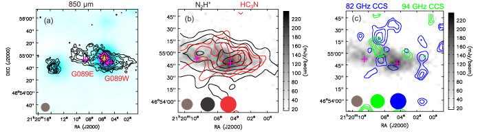
Figure 1: (a) The 850 $\mu$m continuum image (contours) obtained toward G089.9-01.9 superimposed on the WISE 22 $\mu$m image (color). Contour levels are [0.2, 0.3, 0.4, 0.5, 0.6, 0.7, 0.8, 0.9] $\times$ 235.7 mJy/beam. The magenta cross symbol represents the SCUBA-2 peak position (Table 3). The dark brown filled circle represents the half-power beam size for JCMT/SCUBA-2 850 $\mu$m. (b) Black and red contour maps represent N₂H⁺ and HC₃N integrated intensity maps, respectively, while the gray-scale map represents the 850 $\mu$m continuum intensity. The N₂H⁺ integrated intensity is calculated for the main hyperfine component group $F_{1}$ = 2$-$1 ($F$ = 1$-$0, 2$-$1, and 3$-$2) from a velocity range of 0.5 to 3.5 km s^-1 with levels of [3, 6, 9, 12, 15] $\times$ 0.092 K km s^-1(1$\sigma$). The HC₃N intensity is calculated from a velocity range of 0.5 to 3.5 km s^-1 with levels of [3, 4.5, 6, 7.5, 10] $\times$ 0.081 K km s^-1(1$\sigma$). The black and red filled circles represent the half-power beam sizes for N₂H⁺ and HC₃N, respectively. (c) Blue and green contours represent the 82 GHZ CCS and 94 GHz CCS integrated intensity maps, respectively, while the gray-scale map represents the 850 $\mu$m continuum intensity. The 82 GHz CCS intensity is calculated from a velocity range of 0.5 to 3.5 km s^-1 with levels of [2.5, 3, 3.5, 4] $\times$ 0.080 K km s^-1(1$\sigma$). The 94 GHz CCS intensity is calculated from a velocity range of 0.5 to 3.5 km s^-1 with levels of [2.5, 3, 3.5, 4] $\times$ 0.11 K km s^-1(1$\sigma$). The blue and green filled circles represent the half-power beam sizes for 82 GHz CCS and 94 GHz CCS, respectively.

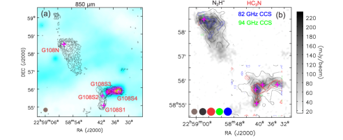
Figure 2: Same as Figure 1 but for G108.8-00.8. (a) The 850 $\mu$m continuum (contours) levels are [0.2, 0.3, 0.4, 0.5, 0.6, 0.7, 0.8, 0.9] $\times$ 231.9 mJy/beam. (b) For G108N, The N₂H⁺ intensity (black contours) is calculated from a velocity range of -51.5 to -47.5 km s^-1 with levels of [3, 6, 9, 12, 15] $\times$ 0.088 K km s^-1(1$\sigma$). For G108S, the N₂H⁺ intensity (black contours) is calculated from a velocity range of -52.5 to -48.5 km s^-1 with levels of [3, 6, 9, 12, 15] $\times$ 0.066 K km s^-1(1$\sigma$). For G108N, the HC₃N intensity (red) is calculated from a velocity range of -51.5 to -47.5 km s^-1 with levels of 2.5 $\times$ 0.078 K km s^-1(1$\sigma$). For G108S, the HC₃N intensity (red) is calculated from a velocity range of -52.5 to -48.5 km s^-1 with levels of [2.5, 3, 4, 5, 6] $\times$ 0.064 K km s^-1(1$\sigma$). For G108N, the 82 GHz CCS intensity (blue) is calculated from a velocity range of -51.5 to -47.5 km s^-1 with levels of [2.5, 3, 3.5, 4, 4.5] $\times$ 0.080 K km s^-1(1$\sigma$). For G108S, the 82 GHz CCS intensity (blue) is calculated from a velocity range of -52.5 to -48.5 km s^-1 with levels of [2.5, 3, 3.5, 4, 4.5] $\times$ 0.078 K km s^-1(1$\sigma$). For G108N, the 94 GHz CCS intensity (green) is calculated from a velocity range of -51.5 to -47.5 km s^-1 with levels of 2.5 $\times$ 0.11 K km s^-1(1$\sigma$). For G108S, the 94 GHz CCS intensity (green) is calculated from a velocity range of -52.5 to -48.5 km s^-1 with levels of 2.5 $\times$ 0.076 K km s^-1(1$\sigma$).

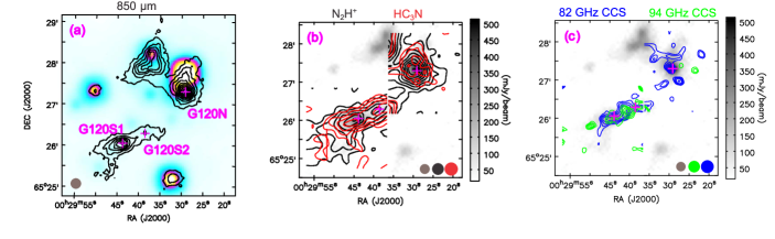
Figure 3: Same as Figure 1 but for G120.7+2.7. (a) The 850 $\mu$m continuum (contours) levels are [0.1, 0.2, 0.3, 0.4, 0.5, 0.6, 0.7, 0.8, 0.9] $\times$ 514.4 mJy/beam. (b) For G120N, The N₂H⁺ intensity (black contours) is calculated from a velocity range of -19.5 to -15.5 km s^-1 with levels of [3, 6, 9, 12, 15, 18, 21, 24, 27] $\times$ 0.098 K km s^-1(1$\sigma$). For G120S, The N₂H⁺ intensity (black contours) is calculated from a velocity range of -19.5 to -16.5 km s^-1 with levels of [2.5, 3, 3.5, 4, 4.5, 5, 6, 7] $\times$ 0.099 K km s^-1(1$\sigma$). For G120N, The HC₃N intensity (red) is calculated from a velocity range of -19.5 to -15.5 km s^-1 with levels of [3, 4.5, 6] $\times$ 0.090 K km s^-1(1$\sigma$). For G120S, The HC₃N intensity (red) is calculated from a velocity range of -19.5 to -16.5 km s^-1 with levels of [3, 6, 9, 12] $\times$ 0.062 K km s^-1(1$\sigma$). (c) For G120N, The 82 GHz CCS intensity (blue) is calculated from a velocity range of -19.5 to -15.5 km s^-1 with levels of [2.5, 3, 3.5, 4, 4.5] $\times$ 0.1 K km s^-1(1$\sigma$). For G120S, The 82 GHz CCS intensity (blue) is calculated from a velocity range of -19.5 to -16.5 km s^-1 with levels of [3, 3.5, 4, 4.5, 5] $\times$ 0.080 K km s^-1(1$\sigma$). For G120N, The 94 GHz CCS intensity (green) is calculated from a velocity range of -19.5 to -15.5 km s^-1 with levels of [2.5, 3, 3.5] $\times$ 0.11 K km s^-1(1$\sigma$). For G120S, The 94 GHz CCS intensity (green) is calculated from a velocity range of -19.5 to -16.5 km s^-1 with levels of [3, 3.5, 4, 4.5, 5] $\times$ 0.085 K km s^-1(1$\sigma$).

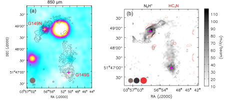
Figure 4: Same as Figure 1 but for G149.5-1.2. (a) The 850 $\mu$m continuum (contours) levels are [0.2, 0.3, 0.4, 0.5, 0.6, 0.7, 0.8, 0.9] $\times$ 117.2 mJy/beam. (b) The N₂H⁺ intensity (black contours) is calculated from a velocity range of -8.5 to -5.5 km s^-1 with levels of [2.5, 3, 3.5, 4, 4.5, 5, 6, 7] $\times$ 0.099 K km s^-1(1$\sigma$). The HC₃N intensity (red) is calculated for a velocity range of -8.5 to -5.5 km s^-1 with levels of [2.5, 3] $\times$ 0.080 K km s^-1(1$\sigma$).

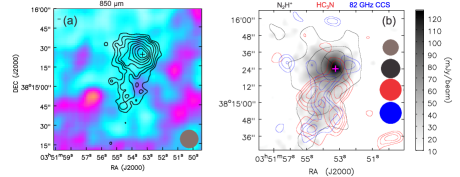
Figure 5: Same as Figure 1 but for G157.6-12.2. (a) The 850 $\mu$m continuum (contours) levels are [0.2, 0.3, 0.4, 0.5, 0.6, 0.7, 0.8, 0.9] $\times$ 126.8 mJy/beam. (b) The N₂H⁺ intensity (black contours) is calculated from a velocity range of -8.5 to -6.5 km s^-1 with levels of [3, 6, 9] $\times$ 0.078 K km s^-1(1$\sigma$). The HC₃N intensity (red) is calculated from a velocity range of -8.5 to -6.5 km s^-1 with levels of [2.5, 3, 3.5, 4] $\times$ 0.071 K km s^-1(1$\sigma$). The 82 GHz CCS intensity (blue) is calculated from a velocity range of -8.5 to -6.5 km s^-1 with levels of [2.5, 3, 3.5] $\times$ 0.086 K km s^-1(1$\sigma$).

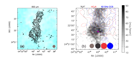
Figure 6: Same as Figure 1 but for G174.0-15.8. (a) The 850 $\mu$m continuum (contours) levels are [0.3, 0.4, 0.5, 0.6, 0.7, 0.8, 0.9] $\times$ 90.3 mJy/beam. (b) Black contours representintensity integrated for a velocity range of 5.5 to 7.5 km s^-1 with levels of [3, 4.5, 6] $\times$ 0.065 K km s^-1(1$\sigma$). The HC₃N intensity (red) is calculated from a velocity range of 5.5 to 7.5 km s^-1 with levels of [3, 6, 9, 12] $\times$ 0.052 K km s^-1(1$\sigma$). The 82 GHz CCS intensity (blue) is calculated from a velocity range of 5.5 to 7.5 km s^-1 with levels of [3, 4.5, 6] $\times$ 0.065 K km s^-1(1$\sigma$).

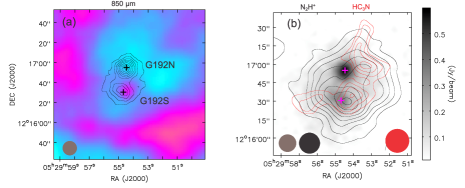
Figure 7: Same as Figure 1 but for G192.32-11.88. (a) The 850 $\mu$m continuum (contours) levels are [0.2, 0.3, 0.4, 0.5, 0.6, 0.7, 0.8, 0.9] $\times$ 600 mJy/beam. (b) The N₂H⁺ intensity (black contours) is calculated from a velocity range of 11.5 to 13.5 km s^-1 with levels of [3, 6, 9, 12, 15, 18, 21, 24] $\times$ 0.081 K km s^-1(1$\sigma$). The HC₃N intensity (red) is calculated from a velocity range of 11.5 to 13.5 km s^-1 with levels of [3, 4, 5, 6] $\times$ 0.069 K km s^-1(1$\sigma$).

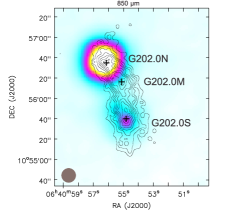
Figure 8: The 850 $\mu$m continuum image (contours) obtained with JCMT/SCUBA-2 toward G202.00+2.65 superimposed on the WISE 22 $\mu$m image (color). Contour levels are [0.2, 0.3, 0.4, 0.5, 0.6, 0.7, 0.8, 0.9] $\times$ 88.8 mJy/beam.

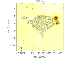
Figure 9: Same as Figure 8 but for G202.31-8.92. Contour levels are [0.2, 0.3, 0.4, 0.5, 0.6, 0.7, 0.8, 0.9] $\times$ 231.2 mJy/beam.

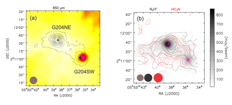
Figure 10: Same as Figure 1 but for G204.4-11.3. (a) The 850 $\mu$m continuum (contours) levels are [0.1, 0.2, 0.3, 0.4, 0.5, 0.6, 0.7, 0.8, 0.9] $\times$ 861.5 mJy/beam. (b) The N₂H⁺ intensity (black contours) is calculated from a velocity range of 0.5 to 2.5 km s^-1 with levels of [3, 6, 9, 12, 15] $\times$ 0.11 K km s^-1(1$\sigma$). The HC₃N intensity (red) is calculated for intensity integrated for a velocity range of 0.5 to 2.5 km s^-1 with levels of [3, 4.5, 6, 7.5, 10] $\times$ 0.086 K km s^-1(1$\sigma$).

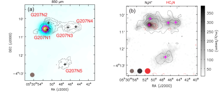
Figure 11: Same as Figure 1 but for G207N. (a) The 850 $\mu$m continuum (contours) levels are [0.1, 0.2, 0.3, 0.4, 0.5, 0.6, 0.7, 0.8, 0.9] $\times$ 386.4 mJy/beam. (b) The N₂H⁺ intensity (black contours) is calculated from a velocity range of 9.5 to 12.5 km s^-1 with levels of [3, 6, 9, 12, 15, 18] $\times$ 0.13 K km s^-1(1$\sigma$). The HC₃N intensity (red) is calculated for intensity integrated for a velocity range of 9.5 to 12.5 km s^-1 with levels of [3, 4.5, 6, 7.5] $\times$ 0.11 K km s^-1(1$\sigma$).

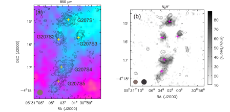
Figure 12: Same as Figure 1 but for G207S. (a)The 850 $\mu$m continuum (contours) levels are [0.2, 0.3, 0.4, 0.5, 0.6, 0.7, 0.8, 0.9] $\times$ 88.8 mJy/beam. (b) The N₂H⁺ intensity (black contours) is calculated from a velocity range of 11.5 to 12.5 km s^-1 with levels of [2.5, 3, 3.5, 4, 4.5, 5] $\times$ 0.083 K km s^-1(1$\sigma$).

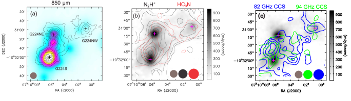
Figure 13: Same as Figure 1 but for G224.4-0.6. (a) The 850 $\mu$m continuum (contours) levels are [0.1, 0.2, 0.3, 0.4, 0.5, 0.6, 0.7, 0.8, 0.9] $\times$ 946.5 mJy/beam. (b) The N₂H⁺ intensity (black contours) is calculated from a velocity range of 12.5 to 17.5 km s^-1 with levels of [3, 5, 10, 15, 20, 25, 30] $\times$ 0.15 K km s^-1(1$\sigma$). The HC₃N intensity (red) is calculated from a velocity range of 12.5 to 17.5 km s^-1 with levels of [3, 6, 9, 12] $\times$ 0.12 K km s^-1(1$\sigma$). (c) The 82 GHz CCS intensity (blue) is calculated for a velocity range of 12.5 to 17.5 km s^-1 with levels of [3, 4.5, 6, 7.5] $\times$ 0.13 K km s^-1. The 94 GHz CCS intensity (green) is calculated from a velocity range of 12.5 to 17.5 km s^-1 with levels of [3, 4.5, 6] $\times$ 0.14 K km s^-1(1$\sigma$).

4 Individual Objects

4.1 G089.9-01.9

The object is located in L974 (Lynds, 1962; Dobashi et al., 2005), and in the dark cloud Khavtassi 137 (Khavtassi, 1960). There is a Class 0 like source (IRAS 21182+4611), which is a bright source in the WISE image, northeast of the western core G089W with an offset of $\sim$ 15$\arcsec$. Then, we regard G089W itself as starless. To our knowledge, there is no information that the eastern core G089E is associated with any young stellar object, and we also regard it as starless. Figure 1 shows maps toward G089.9-01.9. The N₂H⁺ distribution shows a resemblance to the 850 $\mu$m distribution, but their peak positions are slightly different. The HC₃N distribution shows some similarity to the 850 $\mu$m distribution, but the correlation between their intensities is poor. The 82 GHz CCS distribution is very clumpy, and appears as if it surrounds the 850 $\mu$m core. The 94 GHz CCS distribution is different, but it is still located on both sides of the 850 $\mu$m core. Nobeyama T70 observations were made toward G089W. The column density ratio of $N$(DNC) to $N$(HN¹³C) is 4.5, which is close to the value of 3.0 at L1544 (Hirota, Ikeda, & Yamamoto, 2003; Hirota & Yamamoto, 2006). L1544 is known as a prestellar core showing collapsing motion (Tafalla et al., 1998).

4.2 G108.8-00.8

G108.8-00.8 is located in a GMC (1$\arcdeg\times 15\arcmin$) associated with five Sharpless (1959) Hii regions, S147, S148, S149, S152, and S153, and also associated with the supernova remnant G109.1-1.0 (CTB109) in the Perseus arm (Tatematsu et al., 1985, 1987). These two cores are located between peaks $\alpha$ (corresponding to S152) and $\zeta$ in Tatematsu et al. (1985). G108.8-00.8S is associated with two Class I-like sources seen in the WISE image, while G108.8-00.8N is starless. Figure 2 shows maps toward G108.8-00.8. The N₂H⁺ distribution resembles the 850 $\mu$m distribution. The HC₃N emission is observed at the edge of the 850 $\mu$m core of G108N , and the correlation between N₂H⁺ and HC₃N is poor. For G108S, their distributions are more or less correlated. The 82 GHz CCS emission is detected toward the N₂H⁺/850 $\mu$m cores (G108N and G108S) and also the edge of them (G108N). Note that this source is distant, the spatial resolution is as large as 0.3 pc. It is possible that different distributions between N₂H⁺ and CCS are less clear due to its large distance. The kinetic temperature of G108S is 14.3$\pm$3.0 K. G108S is as cold as typical cold dark clouds. Nobeyama T70 observations were made toward G108N, a starless core. We detected DNC, but not HN¹³C. The column density ratio of $N$(DNC) to $N$(HN¹³C) is $>$ 2.5, which is similar to the value of 3.0 at L1544 (Hirota, Ikeda, & Yamamoto, 2003; Hirota & Yamamoto, 2006). See also Kim et al. (2016) for our observations with other telescopes such as PMO 14m, CSO, IRAM 30 m telescopes, etc.

4.3 G120.7+2.7

Figure 3 shows maps toward G120.7+2.7. The WISE source is clearly offset from G120N, and we regard the latter as a starless core. Both N₂H⁺ and HC₃N distributions are well correlated with the 850 $\mu$m distribution. In G120N, the 82 GHz CCS emission has two intensity peaks, and one of them is close to the N₂H⁺ emission peak. Toward the N₂H⁺ peak, we detected N₂D⁺. In G120S, the N₂H⁺ emission shows two cores. We clearly detected both 82GHz and 94GHz CCS emission at G120S. It is possible that the CCS emission surrounds the N₂H⁺ cores, although it is less clear. Nobeyama T70 observations were made toward G120N, a starless core. The column density ratio of $N$(DNC) to $N$(HN¹³C) is 1.7, which is close to the value of 1.91 at L1498 (Hirota & Yamamoto, 2006).

4.4 G149.5-1.2

This clump is located at the edge of the dark cloud Khavtassi 241 (Khavtassi, 1960). Figure 4 shows maps toward G149.5-1.2. The N₂H⁺ distribution is well correlated with the 850 $\mu$m distribution. The HC₃N emission is poorly correlated with the 850 $\mu$m distribution, and it is located on both sides of the north-eastern 850 $\mu$m (and N₂H⁺) core. We detected the N₂D⁺ emission in single pointing observations between the brightest N₂H⁺ core G149N (WISE source) and the northern HC₃N core. The column density ratio of $N$(DNC) to $N$(HN¹³C) is 3.2, which is close to the value of 3.0 in L1544 (Hirota, Ikeda, & Yamamoto, 2003; Hirota & Yamamoto, 2006).

4.5 G157.6-12.2

This clump is located near the dark cloud L1449 (Lynds, 1962; Dobashi et al., 2005) and in Khavtassi 257 (Khavtassi, 1960), which is close to the California Nebula, NGC 1499. Figure 5 shows maps toward G157.6-12.2. The N₂H⁺ distribution is well correlated with the 850 $\mu$m distribution. The 82 GHz CCS emission surrounds the 850 $\mu$m (and N₂H⁺) core. The HC₃N emission shows distribution different from the N₂H⁺ distribution, and looks anticorrelated with the 82 GHz CCS emission. Nobeyama T70 observations were made toward the center of G157, a starless core. The column density ratio of $N$(DNC) to $N$(HN¹³C) is 6.9, which is larger than the value of 3.0 at L1544 (Hirota, Ikeda, & Yamamoto, 2003; Hirota & Yamamoto, 2006).

4.6 G174.0-15.8

This clump is located in L1529 (Lynds, 1962; Wouterloot & Habing, 1985; Dobashi et al., 2005) in Taurus. G174.0-15.8 is a starless clump. Figure 6 shows maps toward G174.0-15.8. The N₂H⁺ distribution is more or less correlated with the 850 $\mu$m distribution. The HC₃N and 82 GHz CCS emission is distributed more extensively than the 850 $\mu$m core.

4.7 G192.32-11.88

G192.3-11.8 is located in the $\lambda$ Orionis complex, and is associated with B30 cataloged by Barnard (1927), L1581 (Lynds, 1962; Dobashi et al., 2005), and with No. 9 CO emission peak identified by Maddalena et al. (1986). It is located in the dark cloud Khavtassi 296 (Khavtassi, 1960). Liu et al. (2016) discovered an extremely young Class 0 protostellar object (G192N) and a proto-brown dwarf candidate (G192S). Observations with SMA show the existence of molecular outflows associated with these objects. Figure 7 shows maps toward G192.32-11.88. The N₂H⁺ distribution shows an intensity peak toward G192S, while there is no N₂H⁺ peak corresponding to G192N. The 850 $\mu$m map of SCUBA-2 has two clear peaks, G192N being the more intense one. The HC₃N distribution is very different from that of 850 $\micron$ (and N₂H⁺), and is clumpy. G192S is associated with one HC₃N core, while there is no HC₃N counterpart to G192N. It seems that the 850 $\micron$ (and N₂H⁺) peak is surrounded by HC₃N cores.

Liu et al. (2016) detected large velocity gradient in this region in ¹³CO $J$ = 1$-$0 and 2$-$1 in the NE-SW direction, and attributed its origin to compression by the Hii region. The N₂H⁺ core inside shows an E-W velocity gradient of the order of 0.5 km s^-1 arcmin ^-1 or 4 km s^-1 pc ^-1. This gradient is consistent with what was observed by Liu et al. (2016) toward the center of their Clump-S in ¹³CO $J$ = 1$-$0 and 2$-$1 (see their Figure 2). Figure 14 shows the intensity-weighted radial velocity (moment 1) map toward G192.32-11.88 in the N₂H⁺ main hyperfine emission group $F_{1}$ = 2$-$1 ($F$ = 1$-$0, 2$-$1, and 3$-$2). This shows a velocity gradient of 0.5 km s^-1 across the clump in the E-W direction. Because this object is located in the Orion region, where the specific angular momentum was statistically investigated by Tatematsu et al. (2016), and also because this core shows a clear velocity gradient, we investigate its properties in detail. It is well known that the specific angular momentum (angular momentum per unit mass) $J/M$ is roughly proportional to $R^{1.6}$ for molecular clouds and their cores having sizes of 0.1 to 30 pc in general (Goldsmith & Arquilla, 1985; Goodman et al., 1993; Bodenheimer, 1995). We compare the radius, velocity gradient, and the specific angular momentum among these emission lines. The beam-corrected half-intensity radius $R$ is 0.26, 0.16, and 0.058 pc, the velocity gradient is 3.9, 2.2, and 0.23 km s^-1, and $J/M$ is $1.3\times 10^{23}$, $4.5\times 10^{22}$, and $1.7\times 10^{21}$ cm² s^-1, respectively, in ¹³CO $J$ = 1$-$0 and 2$-$1 (Liu et al., 2016) and N₂H⁺ (this study). Tatematsu et al. (2016) investigated the specific angular momentum $J/M$ of N₂H⁺ cores in the Orion A GMC, and compared them with cold cloud cores observed in NH₃ by Goodman et al. (1993). Figure 15 plots the specific angular momentum $J/M$ of G192.32-11.88 cores observed in this study as well as Tatematsu et al. (2016); Goodman et al. (1993).. $J/M$ of G192.32-11.88 in N₂H⁺ is within the range found for cores in the Orion A GMC, but is located at the high end of it. It is possible that compression by the Hii region has resulted in relatively large $J/M$ found in the present study.

Nobeyama T70 observations were made toward G192N associated with the Class 0 like protostar. The column density ratio of $N$(DNC) to $N$(HN¹³C) is 5.8, which is larger than the value of 3.0 at L1544 (Hirota, Ikeda, & Yamamoto, 2003; Hirota & Yamamoto, 2006). Detection of DNC and N₂D⁺ indicates that this core is chemically relatively young, although the core is star forming.

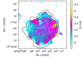
Figure 14: The intensity-weighted radial velocity (moment 1) map (color) toward G192.32-11.88 in the N₂H⁺ $J=1-0$ $F_{1}$ = 2$-$1 main hyperfine emission group $F_{1}$ = 2$-$1 ($F$ = 1$-$0, 2$-$1, and 3$-$2) overlaid on the integrated intensity (moment 0) contour map. The emission less than 2$\sigma$ is ignored in the moment 1 calculation. The contour levels are the same as those in Figure 7.

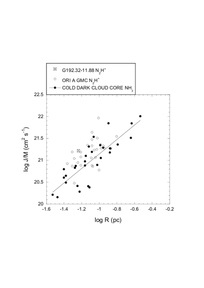
Figure 15: $J/M-R$ diagram for G192.32-11.88 in N₂H⁺ in this study (box with cross), Orion A GMC cores (open circles, Tatematsu et al. (2016)), and cold dark cloud cores (filled circles, Goodman et al. (1993)). The thin solid straight line is computed using a linear least-squares program for cold dark cloud cores.

4.8 G202.00+2.65

This clump is located in the dark cloud L1613 (Lynds, 1962; Dobashi et al., 2005) and Khavtassi 308 (Khavtassi, 1960). $T_{k}$ is derived to be $<$10.2 K. Figure 8 shows the continuum map. The upper limit to the kinetic temperature (10.2 K) was obtained from NH₃ observations.

4.9 G202.31-8.92

G202.31-8.92 is located in L1611 Lynds (1962); Dobashi et al. (2005) in the Orion Northern Filament, and close to No. 52 CO Emission Peak cataloged by Maddalena et al. (1986), which has two CO velocity components 8.8 and 11.4 km s^-1. As Maddalena et al. (1986) discussed, we assume that the distance to G202.31-8.92 is similar to that of Orion A and B GMCs. Figure 9 shows the continuum map. $T_{k}$ is derived to be $<$11.6 K. Two velocity components (9.2 and 12.0 km s^-1) were detected in the ¹²CO (1-0) and ¹³CO (1-0) emission toward this source (Liu et al., 2012). The continuum emission shows a morphology similar to that of the 12.0 km s^-1 CO clump. The velocity of the NH₃ emission is 11.92 km s^-1, which is similar to that of the 12.0 km s^-1 CO clump.

The upper limit to the kinetic temperature (11.6 K) was obtained from NH₃ observations.

4.10 G204.4-11.3

G204.4-11.3 is located in L1621 Lynds (1962); Dobashi et al. (2005) and the Orion B GMC, and close to No.37 CO Emission Peak cataloged by Lynds (1962); Maddalena et al. (1986), which has two CO velocity components 8.6 and 10.9 km s^-1. It is located near the edge of the dark cloud Khavtassi 311 (Khavtassi, 1960). As Maddalena et al. (1986) discussed, we assume that the distance to G204.4-11.3 is similar to that of Orion A and B GMCs. Figure 10 shows maps toward G204-11.3. The N₂H⁺ emission shows a peak toward the starless peak G204NE in the 850 $\mu$m continuum, but with a marginal offset of $\sim 10\arcsec$. The HC₃N is more extended than 850 $\mu$m (and N₂H⁺). Toward G204NE (virtually identical to the T70 position), we detected the 82 GHz CCS emission (Tables 4 and 5), but the emission is too weak and narrow to draw a reliable map. In the single pointing observations toward G204NE, we have detected both DNC and N₂D⁺. The column density ratio of $N$(DNC) to $N$(HN¹³C) is 15.0, which is much larger than the value of 3.0 at L1544 (Hirota, Ikeda, & Yamamoto, 2003; Hirota & Yamamoto, 2006). The high deuterium fraction ratio implies that G204NE is a starless core on the verge of star formation. Figure 16 shows the moment 1 radial velocity map toward G204-11.3 in N₂H⁺. We do not see a prominent velocity gradient ($<$ 0.5 km s^-1 arcmin^-1 or $<$4 km s^-1 pc^-1).

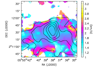
Figure 16: The radial velocity (moment 1) map (color) toward G204.4-11.3 in N₂H⁺ superimposed on the integrated intensity (moment 0) map. The contour levels are the same as those in Figure 12.

4.11 G207.3-19.8

G207.3-19.8 is located in the Orion A GMC, and close to No. 19 CO emission peak identified by Maddalena et al. (1986). G207N is associated with the Herbig-Haro object HH58, which is a Class 0 like source. G207S is starless. Figure 11 shows maps toward G207N. The N₂H⁺ emission is well correlated with the 850 $\mu$m distribution. The N₂H⁺ emission shows a peak toward G207N1 associated with HH58. The HC₃N also shows a peak toward G207N1. Weak emission is observed also toward G207N2, G207N3, G207N4, and G207N5 in N₂H⁺, but not in HC₃N. We have not detected either the 82 GHz or 94 GHz CCS emission. In single pointing observation toward the T70 position, which was mistakenly set north of G207N, we have not detected either DNC or N₂D⁺.

Figure 12 shows the N₂H⁺ map toward G207S. The N₂H⁺ emission is more or less correlated with the 850 $\mu$m distribution, but their peak positions do not coincide completely with each other. We have not detected either the HC₃N, 82 GHz or 94 GHz CCS emission.

4.12 G224.4-0.6

This clump is located in L1658 Lynds (1962); Dobashi et al. (2005), the Orion Southern Filament (Genzel & Stutzki, 1989), CMa R1 region (Nakano et al., 1984), and CMa OB1 (Blitz, 1978; Kim et al., 1996) and near the dark cloud Khavtassi 330 (Khavtassi, 1960). Figure 13 shows maps toward G224.4-0.6. The N₂H⁺ emission is well correlated with the 850 $\mu$m distribution. Both tracers have two prominent intensity peaks, i.e., G224NE and G224S. We see slight peak position offsets. The HC₃N emission is not well correlated with the 850 $\mu$m distribution, and shows a stronger peak toward the southern 850 $\mu$m source. The 82 GHz and 94 GHz CCS emissions have local emission peaks between the two 850 $\mu$m sources. T70 observations were carried out toward G224NE, and we detected DNC and HN¹³C. Figure 17 shows the moment 1 radial velocity map in N₂H⁺. We see a steep velocity gradient. The SE-NW gradient is about 0.9 km s^-1 arcmin^-1 or 3 km s^-1 pc^-1.

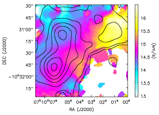
Figure 17: The radial velocity (moment 1) map (color) toward G224.4-0.6 in N₂H⁺ superimposed on the integrated intensity (moment 0) map. The contour levels are the same as those in Figure 16.

5 Discussion

5.1 Column Density Ratios

Hirota & Yamamoto (2006) indicated the evolutionary sequence of starless cores by using column density ratios such as $N$(DNC)/$N$(HN¹³C). It seems that $N$(DNC)/$N$(HN¹³C) in starless cores increases with core evolution ($<$0.66 to 3). Using their data, we can show that $N$(N₂H⁺)/$N$(CCS) is $\lesssim$ 0.12 for young starless cores (L1495B, L1521B, L1521E, TMC-1, and L492). According to Tatematsu et al. (2014a), $N$(N₂H⁺)/$N$(CCS) is usually $\lesssim 2-3$ for starless cores, but can reach $\sim$ 2$-$3 for evolved starless cores. Star-forming cores generally give $N$(N₂H⁺)/$N$(CCS) $\gtrsim 2-3$.

In the present observations, $N$(N₂H⁺)/$N$(CCS) ranges from 0.4 to 3.7, and $N$(DNC)/$N$(HN¹³C) ranges from 1.7 to 10. These results suggest that our Planck cold clumps consist of various evolutionary stages including relatively young starless cores and those on the verge of star formation. In the present observations, $N$(N₂D⁺)/$N$(N₂H⁺) ranges from 0.1 to 1.4. Fontani et al. (2006) and Chen et al. (2011) studied the column density ratio of N₂D⁺ to N₂H⁺ (they call this the deuterium fractionation $D_{frac}$) toward massive protostellar cores, and compared it with those of low-mass prestellar cores by Crapsi et al. (2005). $N$(N₂D⁺)/$N$(N₂H⁺) is of order 10^-1 in low-mass prestellar cores (Crapsi et al., 2005), and of order 10^-2 in massive protostellar IRAS cores (Fontani et al., 2006). The ratio is estimated to be 0.35 and 0.08 at typical cold clouds, L134N and TMC-1N, respectively (Tiné et al., 2000). Our N₂D⁺ detected cores have larger $N$(N₂D⁺)/$N$(N₂H⁺) values than the massive protostellar IRAS cores of Fontani et al. (2006).

In G149.5-1.2 (contains a WISE source), G192N (contains a Class 0), G207N (contains HH58), and G207S, we did not detect the 82 GHz CCS emission over the OTF map regions. The H₂ column density of our sources are 3$\times 10^{21}$ cm^-2 or higher (Tables 10 and 11). In G149.5-1.2, the H₂ column density is lower than 1$\times 10^{22}$ cm^-2. It is possible that a low column density is the reason for non-detection of CCS. The H₂ column density toward G192N (contains Class 0) is as high as 6$\times 10^{22}$ cm^-2, so non-detection of CCS probably means that the gas is chemically evolved. In G108S, the H₂ column density is as low as $\sim 1\times 10^{22}$ cm^-2, but we detected the 82 GHz CCS emission. G089W (starless) should be chemically young, because $N$(N₂H⁺)/$N$(CCS) is as small as 0.7 and $N$(N₂D⁺)/$N$(N₂H⁺) is as high as 1.4. G157.6-12.2 (starless) is young, because $N$(DNC)/$N$(HN¹³C) is as high as 10.4. G108N (starless) and G204NE (starless) show $N$(N₂H⁺)/$N$(CCS) is $\sim$ 2, which is close to the border between starless and star-forming cores in Tatematsu et al. (2014a).

In the next subsection, we discuss the evolutionary stage of our Planck cold clumps on the basis of the column density ratios in Tables 8 and 9. We assume the filling factor is unity when we estimate the column density, but it is possible that the beam filling factor is less than unity. If beam filling factors are similar between molecules, then the column density ratio will be less affected by unknown absolute values of the filling factor. Because $T_{k}$ is $\lesssim$ 25 K in general, we can use $N$(N₂H⁺)/$N$(CCS) as a chemical evolution tracer (Tatematsu et al., 2014a). The beam sizes for CCS and NH₃ differ by a factor of four, and $N$(NH₃)/$N$(CCS) suffers from sampling/averaging over very different size scales. We thus consider $N$(NH₃)/$N$(CCS) much less reliable.

5.2 Chemical Evolution Factor

We introduce a new parameter to represent the chemical evolution by using molecular column density ratios, the chemical evolution factor (CEF). We define CEF so that starless cores have CEFs of $\sim$ -100 to 0, and star-forming cores show $\sim$ 0 to 100. Starless cores having CEF $\sim$ 0 are regarded as being on the verge of star formation. We use the form of CEF = log([$N$(A)/$N$(B)]/[$N_{0}$(A)/$N_{0}$(B)])*$d$ for the column density ratio of molecule A to molecule B. $N_{0}$(A)/$N_{0}$(B) is chosen to be the column density ratio at the time of star formation. For ($N$(N₂H⁺)/$N$(CCS) and $N$(NH₃)/$N$(CCS), $N_{0}$(A)/$N_{0}$(B) corresponds to the border between starless and star-forming cores. For $N$(DNC)/$N$(HN¹³C) and $N$(N₂D⁺)/$N$(N₂H⁺), $N_{0}$(A)/$N_{0}$(B) is the highest value observed for starless cores. The factor $d$ is determined so that all starless cores range approximately from -100 to 0. By taking into account the observational results of Suzuki et al. (1992); Crapsi et al. (2005); Hirota & Yamamoto (2006); Tatematsu et al. (2014a), we define CEF as CEF = log($N$(N₂H⁺)/$N$(CCS)/2.5)*50, log($N$(DNC)/$N$(HN¹³C)/3)*120, log($N$(N₂D⁺)/$N$(N₂H⁺)/0.3)*50, and log($N$(NH₃)/$N$(CCS)/70)*70, for starless cores with $T_{k}$ $\sim$ 10$-$ 20 K at a spatial resolution of order 0.015-0.05 pc (for 0.1-pc sized structure “molecular cloud core”). These expressions should be only valid for the above-mentioned temperature range and spatial resolution, because we determined the CEF by using data obtained for molecular clumps or molecular cloud cores having such temperatures and observed at such spatial resolutions. The chemical reaction will depend on density, temperature, radiation strength, cosmic-ray strength, etc. The deuterium fraction will be lower for warm cores (Snell & Wootten, 1979; Wootten, 1987; Schilke et al., 1992; Tatematsu et al., 2010). It seems that the deuterium fraction decreases after the onset of star formation (Emprechtinger et al., 2009; Sakai et al., 2012; Fontani et al., 2014; Sakai et al., 2015). Because the nature of this decrease has not yet been fully characterized observationally, we do not use star-forming cores for CEF based on the deuterium fractionation. Figure 18 shows the resulting CEF using the data in the literature (Crapsi et al., 2005; Hirota & Yamamoto, 2006; Hirota, Ohishi, & Yamamoto, 2009).

Tables 12 and 13 and Figures 19 and 20 show the CEFs estimated in the present study. We regard cores as star-forming if the first entry of comments in Table 3 suggests a possibility of star formation (e.g., Class 0, Class I etc). Our beam size with receivers TZ1 and T70 corresponds to 0.1 and 0.3 pc at a distance of 700 pc and 3.5 kpc, respectively. To see the effect of very different spatial resolution (and probably very different volume density and very different beam-filling factor), we show sources located beyond 1 kpc in parentheses. In this paper we treat only starless cores for CEF, because evolution of star-forming cores has not well been characterized yet. If we mistakenly identified star-forming cores as starless, we may mistakenly obtain lower CEF due to decrease in the deuterium fractionation after star formation. If this is the case, we may see inconsistency between CEF based on he deuterium fractionation and that based on $N$(N₂H⁺)/$N$(CCS). CEF(average) does not include the upper or lower limit to $N$(N₂H⁺)/$N$(CCS). For G108N, CEF(DNC,HN¹³C) is a lower limit, but because this is a starless core, we will not provide a positive CEF(DNC,HN¹³C) value. That means CEF(DNC,HN¹³C) = -9 to 0 nominally. However, this does not mean the estimate is very accurate. Then, we simply adopt this lower limit value of -9 to avoid being misleading. Figures 19 and 20 show that G174.0-15.8 is chemically young, and G204NE seems to be in the intermediate stage (on the verge of star formation).

The advantage of Planck cold clumps is that they are cold ($\lesssim$ 20 K), and less affected by temperature effects. We have detected the N₂H⁺ (1-0) emission from all the 13 clumps mapped with the Nobeyama 45 m telescope and receiver TZ1. The optically thin critical density for this transition is 6.1$\times 10^{4}$ and 4.1$\times 10^{4}$ cm^-3 for 10 and 20 K, respectively (Shirley, 2015). The volume density $n$ for dense cores in cold molecular clouds detected in N₂H⁺ (1-0) is $\gtrsim$ 3$\times 10^{4}$ cm^-3 (Caselli et al., 2002). Thus, we can assume that the 13 mapped Planck cold clumps have densities higher than $\gtrsim$ 3$\times 10^{4}$ cm^-3. With increasing density, the chemical reaction timescale will decrease. Then, the change in CEF will correspond to longer timescales for lower densities. The physical nature of the Planck cold clumps such as radius, mass, and volume density will be discussed in detail in a separate paper.

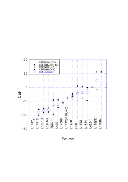
Figure 18: Chemical Evolution Factor (CEF) for starless sources in the literature.

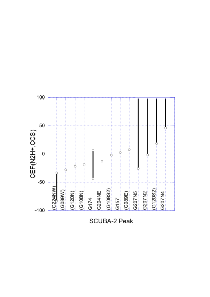
Figure 19: Chemical Evolution Factor (CEF) for starless SCUBA-2 peaks based on the column density ratio of $N$(N₂H⁺)/$N$(CCS). The source name in parentheses means distance is larger than 1kpc. The range reflects the uncertainty for the N₂H⁺ optical depth for cores for which hyperfine fitting was not successful.

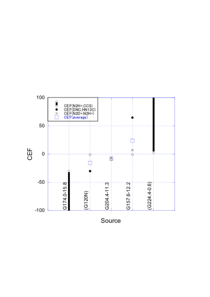
Figure 20: Chemical Evolution Factor (CEF) at starless T70 positions based on multiple column density ratios. The source name in parentheses means distance is larger than 1kpc. The range reflects the upper and lower limit to $N$(N₂H⁺)/$N$(CCS).

5.3 Molecular Distribution

Next, we investigate the morphology. In G089.9-01.9, the 82 GHz and 94 GHz CCS emission (young molecular gas) is distributed as if it surrounds the N₂H⁺ core (evolved gas). In G157.6-12.2, the 82 GHz CCS emission is distributed as if it surrounds the N₂H⁺ core. Such configurations were previously reported in Aikawa et al. (2001) for L1544, and also starless NH₃ core surrounded by CCS configurations are also observed by Lai & Crutcher (2000) for L1498 and Tatematsu et al. (2014b) for Orion A GMC. L1544 shows evidence of the prestellar collapse. Therefore, these cores could be good targets for further studies for the initial conditions of star formation. For G157.6-12.2, CEF is $\gtrsim$ 0, and its linewidth is as narrow as 0.3 km s^-1. It is possible that this core is a coherent core that has largely dissipated turbulence, and is on the verge of star formation (Tatematsu et al., 2014b; Ohashi et al., 2016b). In G120S1, G120S2, and G224.4-0.6 N₂H⁺ and CCS distribution are largely different. G089.9-01.9, G120S, G157.6-12.2 are cold ($<$ 11K), which may suggest depletion of CCS (cf., Aikawa et al. (2001); Bergin et al. (2002); Caselli et al. (2002). On the other hand, N₂H⁺ peaks are detected in the HC₃N emission in these cores. In G149N, the HC₃N emission (young molecular gas) is distributed on the both sides of the N₂H⁺ core (evolved gas), which is also interesting. In G108N and G108S, the 82 GHz GHz CCS and N₂H⁺ emission coexist roughly, but, again, this could be due to poorer physical resolution or a projection effect.

6 Summary

Thirteen Planck cold clumps were observed with the James Clerk Maxwell Telescope/SCUBA-2 and with the Nobeyama 45 m radio telescope. The N₂H⁺ spatial distribution is similar to SCUBA-2 dust distribution. The spatial distribution of HC₃N, 82 GHz CCS, and 94 GHz CCS emission is often different from that of the N₂H⁺ emission. The CCS emission is often very clumpy. In G089.9-01.9 and G157.6-12.2, the CCS emission surrounds the N₂H⁺ core, which resembles the case of L1544 and suggests that they are on the verge of star formation. The detection rate of N₂D⁺ is 50%. We investigated chemical evolutionary stages of starless Planck cold clumps using the newly defined Chemical Evolution Factor (CEF). We found that G174.0-15.8 is chemically young, and G089E, G157.6-12.2, and G204NE seem in the intermediate stage (on the verge of star formation). In addition, we observed NH₃, and determined the kinetic temperature $T_{k}$.

Table 1: Observed Lines

Line	Frequency	Frequency Reference	Upper Energy Level $E_{u}$	Receiver	Observing Mode
CCS $J_{N}$ = 7${}_{6}-6_{5}$	81.505208 GHz	Cummins et al. (1986)	15.3 K	TZ1	OTF
CCS $J_{N}$ = 8${}_{7}-6_{5}$	93.870107 GHz	Yamamoto et al. (1990)	19.9 K	TZ1	OTF
HC3N $J$ = 9$-$8	81.8814614 GHz	Picket et al. (1998)	19.7 K	TZ1	OTF
N2H+ $J$ = 1$-$0	93.1737767 GHz	Caselli & Myers (1995)	4.5 K	TZ1	OTF
DNC $J$ = 1$-$0	76.3057270 GHz	Picket et al. (1998)	T70	3.7 K	single pointing
HN13C $J$ = 1$-$0	87.090859 GHz	Frerking et al. (1979)	4.2 K	T70	single pointing
N2D+ $J$ = 1$-$0	77.1096100 GHz	Picket et al. (1998)	3.7 K	T70	single pointing
cyclic C3H2 $J_{K_{a}K_{c}}$ = 2${}_{12}-$101	85.338906 GHz	Thaddeus et al. (1981)	4.1 K	T70	single pointing
NH3 $(J,K)$ = (1, 1)	23.694495 GHz	Ho & Townes (1983)	23.4 K	H22	single pointing

Table 2: Coordinates for the Observations

Source	OTF Reference Center		OTF area	T70		H22		OFF		Distance
	RA(J2000.0)	Dec(J2000.0)		RA(J2000.0)	Dec(J2000.0)	RA(J2000.0)	Dec(J2000.0)	RA(J2000.0)	Dec(J2000.0)	(kpc)
G089.9-01.9	21:20:04.35	46:54:46.8	$2\arcmin\times 2\arcmin$	21:20:04.35	46:54:46.8	21:20:04.35	46:54:46.8	21:19:20	46:54:00	0.62
G108.8-00.8N (G108N)	22:58:56.2	58:58:21.7	$2\arcmin\times 2\arcmin$	22:58:53.6	58:58:21.7	22:58:56.2	58:58:21.7	22:58:15	59:01:00	3.2
G108.8-00.8S (G108S)	22:58:40.8	58:55:34.4	$2\arcmin\times 2\arcmin$			22:58:40.8	58:55:34.4	22:58:15	59:01:00	3.2
G120.7+2.7N (G120N)	00:29:26.11	65:27:14.3	$2\arcmin\times 2\arcmin$	00:29:29.3	65:27:14.3	00:29:26.11	65:27:14.3	00:29:20	65:20:00	1.82
G120.7+2.7S (G120S)	00:29:46.76	65:25:47.8	$2\arcmin\times 2\arcmin$			00:29:46.76	65:25:47.8	00:29:20	65:20:00	1.82
G149.5-1.2	03:56:53	51:48:00	$3\arcmin\times 3\arcmin$	03:56:57.3	51:49:00	03:56:57.3	51:49:00	03:56:15	51:44:00	0.84
G157.6-12.2	03:51:53.6	38:15:22.6	$2\arcmin\times 2\arcmin$	03:51:53.6	38:15:22.6	03:51:53.6	38:15:22.6	03:51:20	38:10:00	0.45
G174.0-15.8	04:32:45.30	24:21:51.7	$2\arcmin\times 2\arcmin$			04:32:45.30	24:21:51.7	04:33:09.19	24:23:42.7	0.15
G192.33-11.88	05:29:54.16	12:16:53.0	$2\arcmin\times 2\arcmin$	05:29:54.16	12:16:53.0	05:29:54.16	12:16:53.0	05:30:05	12:10:00	0.42
G202.00+2.65	06:40:55.10	10:56:16.2				06:40:55.10	10:56:16.2	06:40:43.93	11:01:40.8	0.76
G202.31-8.92	06:00:10	05:15:00				06:00:10.0	05:15:00.0	06:00:18	05:20:00	0.42
G204.4-11.3	05:55:38.54	02:11:35.6	$2\arcmin\times 2\arcmin$	05:55:38.54	02:11:35.6	05:55:38.54	02:11:35.6	05:55:48.98	02:05:37.0	0.42
G207.3-19.8N (G207N)	05:30:48	-04:11:30	$4\arcmin\times 4\arcmin$	05:30:48.5	-04:09:40.0	05:30:46.5	-04:10:30	05:31:35	-04:12:22	0.42
G207.3-19.8S (G207S)	05:31:03.00	-04:16:20	$4\arcmin\times 4\arcmin$			05:31:03.00	-04:17.05.3	05:31:35	-04:12:22	0.42
G224.4-0.6	07:10:03.83	-10:31:28.21	$2\arcmin\times 2\arcmin$	07:09:59.8	-10:31:18.2	07:10:01.12	-10:30:58.2	07:09:55	-10:28:00	1.1

Table 3: Parameters of SCUBA-2 Peaks

Source	SCUBA-2 peak	RA	DEC	comments
		(J2000)	(J2000)
G089.9-01.9	G089E	21:20:08.5	46:54:52.4	starless
	G089W	21:20:04.4	46:54:47.4	starless? an infrared source IRAS 21182+4641 on the east
G108.8-00.8	G108N	22:58:57.5	58:58:30.2	starless
	G108S1	22:58:40.8	58:55:02.0	starless
	G108S2	22:58:41.1	58:55:37.1	starless
	G108S3	22:58:38.9	58:55:48.1	Class I?
	G108S4	22:58:34.2	58:55:48.2	Class I?
G120.7+2.7	G120S1	00:29:43.8	65:26:03.1	WISE faint source only detected at 3.4 and 4.6 micron,
				no AKARI source, a foreground star?
	G120S2	00:29:38.5	65:26:17.8	starless
	G120N	00:29:29.1	65:27:18.4	starless, offset from infrared sources
G149.5-1.2	G149N	03:56:57.2	51:48:50.0	WISE, class I?
	G149S	03:56:50.4	51:46:57.4	starless
G157.6-12.1	G157	03:51:53.3	38:15:24.3	starless
G174.0-15.8	G174	04:32:44.9	24:21:39.6	starless
G192.33-11.88	G192N	05:29:54.5	12:16:55.0	Class 0
	G192S	05:29:54.7	12:16:30.6	proto-brown dwarf candidate
G202.00+2.65	G202.0N	06:40:56.1	10:56:34.9	Class 0? Spitzer, Akari, WISE
	G202.0M	06:40:55.1	10:56:16.4	starless
	G202.0S	06:40:54.8	10:55:40.1	Class 0? Spitzer, WISE
G202.31-8.92	G202.3	06:00:08.8	05:14:59.6	starless
G204.4-11.3	G204NE	05:55:38.4	02:11:35.5	starless
	G204SW	05:55:35.6	02:11:01.6	class 0?
G207N	G207N1	05:30:51.0	-04:10:36.7	class 0? HH 58? but SCUBA-2 core peak offset from infrared source
	G207N2	05:30:50.8	-04:10:14.3	starless
	G207N3	05:30:46.5	-04:10:29.0	starless
	G207N4	05:30:44.7	-04:10:27.4	starless
	G207N5	05:30:47.1	-04:12:31.3	starless
G207S	G207S1	05:31:02.0	-04:14:56.6	starless
	G207S2	05:31:03.7	-04:15:48.3	starless
	G207S3	05:31:00.3	-04:15:43.6	starless
	G207S4	05:31:03.2	-04:17:00.3	starless
	G207S5	05:31:03.8	-04:17:37.0	starless
G224.4-0.6	G224S	07:10:06.2	-10:32:00.3	IRAS 07077-1026, Akari, WISE, Spitzer
	G224NE	07:10:05.6	-10:31:11.8	Akari, WISE, Spitzer
	G224NW	07:10:00.8	-10:30:58.2	starless

Table 4: Intensities Observed with the Receiver TZ1 toward the SCUBA-2 Peaks

SCUBA-2 peak	82 GHz CCS			94 GHz CCS			HC3N			N2H+
	$T_{A}^{*}$	$V_{LSR}$	$\Delta v$	$T_{A}^{*}$	$V_{LSR}$	$\Delta v$	$T_{A}^{*}$	$V_{LSR}$	$\Delta v$	$T_{A}^{*}$	$V_{LSR}$	$\Delta v$	$T_{ex}$	$\tau$(main)	Integrated Intensity
	(K)	(km s-1)	(km s-1)	(K)	(km s-1)	(km s-1)	(K)	(km s-1)	(km s-1)	(K)	(km s-1)	(km s-1)			(K km s-1)
G089E	0.60	1.94	0.14	0.27	1.80	0.68	0.56	1.82	0.49	0.8	1.82	0.40	4.6 $\pm$ 0.4	6.2 $\pm$ 2.0
G089W	0.51	1.31	0.33	0.43	1.43	0.42	1.08	1.29	0.47	1.1	1.50	0.63	8.7 $\pm$ 4.2	1.4 $\pm$ 1.2
G108N	0.18	-49.38	1.53	$<$ 0.16						0.5	-49.40	1.20	5.8 $\pm$ 3.8	0.9 $\pm$ 1.3
G108S1	0.19	-49.00	0.78				0.28	-48.84	0.33	$<$ 0.10
G108S2	0.18	-49.58	1.44				0.22	-49.66	1.39	0.3	-49.78	1.30	3.4 $\pm$ 0.2	3.2 $\pm$ 1.5
G108S3	$<$ 0.12									0.2	$\sim$-50				0.5
G108S4	$<$ 0.12									0.3	-51.20	1.22	3.8 $\pm$ 0.8	1.9 $\pm$ 1.9
G120S1	0.25	-18.01	1.48	0.21	-18.12	1.48	0.51	-18.22	1.27	0.6	-18.33	1.33	4.8 $\pm$ 0.6	1.9 $\pm$ 0.7
G120S2	$<$ 0.14			$<$ 0.15			0.79	-18.16	0.92	0.4	-18.06	0.98	3.9 $\pm$ 0.3	4.0 $\pm$ 2.0
G120N	0.21	-18.44	0.95	$<$ 0.17			0.39	-18.57	1.20	1.2	-18.46	1.24	22.7 $\pm$ 29.0	0.3 $\pm$ 0.5	2.6
G149N	$<$ 0.16			$<$ 0.19						0.6	-7.51	0.41	4.5 $\pm$ 1.3	3.5 $\pm$ 3.3
G149S	$<$ 0.16			$<$ 0.19						$<$ 0.17
G157	0.57	-7.62	0.28	$<$ 0.19						0.8	-7.63	0.29	4.2 $\pm$ 0.1	16.5 $\pm$ 5.0
G174	0.55	6.27	0.33	$<$ 0.16						0.7	6$-$7				0.5
G192N	$<$ 0.16			$<$ 0.17						0.6	$\sim$6				1.4
G192S	$<$ 0.16			$<$ 0.17			0.37	12.17	0.75	1.3	12.23	0.55	5.7 $\pm$ 0.2	6.2 $\pm$ 0.9
G204NE	0.38	1.74	0.71	$<$ 0.17						1.6	1.57	0.47	6.0 $\pm$ 0.4	7.5 $\pm$ 1.6
G204SW	$<$ 0.21			$<$ 0.20						0.5	1.74	0.76	5.2 $\pm$ 3.1	1.8 $\pm$ 2.9	1.0
G207N1	$<$ 0.22			$<$ 0.22			0.44	10.48	1.20	0.9	10.71	1.10	6.1 $\pm$ 1.8	2.4 $\pm$ 1.8
G207N2	$<$ 0.22			$<$ 0.22						0.8	11.20	0.45	5.6 $\pm$ 1.6	3.6 $\pm$ 2.8
G207N3	$<$ 0.22			$<$ 0.22
G207N4	$<$ 0.22			$<$ 0.22						0.4	11.28	0.54	3.5 $\pm$ 0.1	21.5 $\pm$ 12.4	0.9
G207N5	$<$ 0.22			$<$ 0.22						0.9	$\sim$11				0.7
G224S	0.22	14.44	2.59	$<$ 0.19			0.49	14.4	2.17	1.5	$\sim$15				3.9
G224NE	0.15	13.87	3.46	$<$ 0.19			0.36	13.75	1.46	1.6	13.95	1.46	13.6 $\pm$ 4.2	0.9 $\pm$ 0.4
G224NW	0.23	16.21	3.04	$<$ 0.19			0.74	16.38	2.00	0.6	$\sim$16				0.2

Table 5: Intensities Observed with the Receiver TZ1 toward T70 Position

Source	82 GHz CCS			94 GHz CCS			HC3N			N2H+
	$T_{A}^{*}$	$V_{LSR}$	$\Delta v$	$T_{A}^{*}$	$V_{LSR}$	$\Delta v$	$T_{A}^{*}$	$V_{LSR}$	$\Delta v$	$T_{A}^{*}$	$V_{LSR}$	$\Delta v$	$T_{ex}$	$\tau$(main)
	(K)	(km s-1)	(km s-1)	(K)	(km s-1)	(km s-1)	(K)	(km s-1)	(km s-1)	(K)	(km s-1)	(km s-1)	(K)
G089.9-01.9	0.53	1.32	0.32	0.44	1.44	0.47	1.23	1.29	0.45	1.1	1.49	0.60	9.0 $\pm$ 4.9	1.4 $\pm$ 1.3
G108N	0.16	-49.62	1.56	$<$ 0.16			$<$ 0.12			0.5	-49.89	1.39
G120N	0.21	-18.44	0.95	$<$ 0.17			0.45	-18.65	0.81	1.2	-18.57	1.13	8.1 $\pm$ 1.5	1.6 $\pm$ 0.6
G120S	0.35	-18.42	0.73	0.33	-18.42	0.31	0.80	-18.47	0.66	$<$ 0.14
G149.5-1.2	$<$ 0.16			$<$ 0.19			$<$ 0.14			0.6	-7.51	0.41	4.5 $\pm$ 1.3	3.5 $\pm$ 3.3
G157.6-12.2	0.59	-7.62	0.27	$<$ 0.20			$<$ 0.15			0.9	-7.61	0.29	4.5 $\pm$ 0.2	9.4 $\pm$ 1.9
G174.0-15.8	0.64	6.27	0.44	$<$ 0.16			$<$ 0.11			$<$ 0.15
G192.33-11.88	$<$ 0.16			$<$ 0.17	13.48	0.37	$<$ 0.15			0.7	12.12	1.13	4.9 $\pm$ 0.3	2.7 $\pm$ 0.6
G204.4-11.3	0.38	1.74	0.71	$<$ 0.20			$<$ 0.18			1.4	1.59	0.47	5.6 $\pm$ 0.2	8.6 $\pm$ 1.5
G207N	$<$ 0.22			$<$ 0.24			$<$ 0.19			$<$ 0.23
G224.4-0.6	$<$ 0.18			$<$ 0.19			$<$ 0.17			1.6	13.95	1.46	13.6 $\pm$ 4.2	0.9 $\pm$ 0.4

Table 6: Intensities Observed with the Receiver T70

Source	DNC			HN13C			N2D+					c-C3H2
	$T_{A}^{*}$	$V_{LSR}$	$\Delta v$	$T_{A}^{*}$	$V_{LSR}$	$\Delta v$	$T_{A}^{*}$	$V_{LSR}$	$\Delta v$	$T_{ex}$	$\tau$(tau)	$T_{A}^{*}$	$V_{LSR}$	$\Delta v$
	(K)	(km s-1)	(km s-1)	(K)	(km s-1)	(km s-1)	(K)	(km s-1)	(km s-1)	(K)		(K)	(km s-1)	(km s-1)
G089.9-01.9	0.90	1.49	1.19	0.44	1.49	0.79	0.23	1.50	0.50	3.7 $\pm$ 0.4	2.09 $\pm$ 1.08	0.69	1.39	0.78
G108N	0.18	-49.46	2.48	$<$ 0.089		2.48	$<$ 0.036					0.21	-49.84	0.95
G120N	0.30	-18.52	1.51	0.25	-18.46	1.353	0.05 $<$ 0.036					0.51	-18.45	1.41
G149.5-1.2	0.17	-7.47	1.00	0.12	-7.31	0.592	0.05 $<$ 0.036					0.28	-7.44	0.46
G157.6-12.2	1.34	-7.66	0.90	0.53	-7.55	0.564	0.45	-7.65	0.31	4.1 $\pm$ 0.2	3.42 $\pm$ 0.66	1.25	-7.61	0.35
G174.0-15.8
G192.33-11.88	0.81	12.14	1.06	0.22	12.32	0.959	0.28	12.16	0.59	5.8 $\pm$ 2.0	0.58 $\pm$ 0.40	0.42	12.19	0.84
G204.4-11.3	1.69	1.64	1.03	0.74	1.70	0.79	0.38	1.63	0.52	4.7 $\pm$ 1.4	1.68 $\pm$ 1.33	1.47	1.64	0.66
G207N	$<$ 0.040			$<$ 0.026			$<$ 0.036					0.05	11.12	1.64
G224.4-0.6	0.23	15.76	1.42	0.17	15.73	0.479	$<$ 0.044					0.19	15.69	1.35

Table 7: NH₃ Intensities Observed with the Receiver H22 and Derived Rotation and Kinetic Temperatures

Source	NH3 (1,1)			NH3 (2,2)	$T_{rot}$	$T_{k}$
	$T_{A}^{*}$	$V_{LSR}$	$\Delta v$	$T_{A}^{*}$
	(K)	(km s-1)	(km s-1)	(K)	(K)	(K)
G089.9-01.9	0.87	1.59	0.86	0.11	10.5 $\pm$ 0.9	11.0 $\pm$ 1.1
G108N	0.49	-49.56	1.65	0.10	13.1 $\pm$ 2.8	14.3 $\pm$ 3.6
G108S	0.22	-49.82	2.06	$<$ 0.03	$<$ 16.5	$<$ 19.1
G120N	0.42	-18.39	1.61	0.11	13.1 $\pm$ 4.1	14.3 $\pm$ 5.4
G120S	0.57	-18.47	1.11	0.15	11.3 $\pm$ 1.5	12.1 $\pm$ 1.9
G149.5-1.2	0.35	-7.49	0.96	$<$ 0.03	$<$ 13.4	$<$ 14.8
G157.6-12.2	0.71	-7.68	0.72	$<$ 0.03	$<$ 10.7	$<$ 11.4
G174.0-15.8	0.99	6.19	0.81	$<$ 0.03	$<$+ 10.5	$<$ 11.1
G192.33-11.88	1.01	12.06	0.90	0.21	11.6 $\pm$ 1.7	12.5 $\pm$ 2.1
G202.00+2.65	0.80	5.08	0.77	$<$ 0.06	$<$ 9.8	$<$ 10.2
G202.31-8.92	0.60	11.92	0.89	$<$ 0.03	$<$ 10.9	$<$ 11.6
G204.4-11.3	1.34	1.56	0.73	0.14	9.8 $\pm$ 0.7	10.2 $\pm$ 0.8
G207N	0.87	11.04	1.04	0.14	12.9 $\pm$ 5.6	14.1 $\pm$ 7.3
G207S	0.62	11.58	1.31	$<$ 0.04	11.1 $\pm$ 5.3	11.8 $\pm$ 6.5
G224.4-0.6	0.37	14.99	2.72	0.11	14 $\pm$ 13	15.5 $\pm$ 17.7

Table 8: Column Densities and Their Ratios toward SCUBA-2 Peak

SCUBA-2 peak	$N$(CCS)	$N$(N2H+)	$N$(N2H+)/$N$(CCS)
	(cm-2)	(cm-2)
G089E	3.5E+12	1.2E+13	3.6
G089W	6.4E+12	4.5E+12	0.7
G108N	5.2E+12	5.4E+12	1.0
G108S1	6.4E+12
G108S2	1.1E+13	2.5E+13	2.3
G108S3	$<$ 4.9E+12	1.7E+12 $-$ 1.7E+13	$>$ 0.3
G108S4	$<$ 4.9E+12	1.3E+13	$>$ 2.6
G120S1	9.8E+12	1.3E+13	1.3
G120S2	$<$ 3.5E+12	2.1E+13	$>$ 5.9
G120N	3.8E+12	3.5E+12	0.9
G149N	$<$ 6.8E+12	7.2E+12	$>$ 1.1
G149S	$<$ 6.8E+12
G157	8.9E+12	2.5E+13	2.8
G174	5.0E+12	1.7E+12 $-$ 1.7E+13	0.3 $-$ 3.3
G192N	$<$ 3.9E+12	4.6E+12 $-$ 4.6E+13	$>$ 1.2
G192S	$<$ 6.9E+12	1.7E+13	$>$ 2.4
G204NE	1.2E+13	1.7E+13	1.4
G204SW		6.7E+12
G207N1	$<$ 3.3E+12	1.2E+13	$>$ 3.8
G207N2	$<$ 3.3E+12	7.7E+12	$>$ 2.3
G207N3	$<$ 3.3E+12
G207N4	$<$ 3.3E+12	6.8E+13	$>$ 21
G207N5	$<$ 3.3E+12	2.6E+12 $-$ 2.6E+13	$>$ 0.8
G224S	9.6E+12	1.4E+13 $-$ 1.4E+14	1.5 $-$ 15
G224NE	8.6E+12	7.7E+12	0.9
G224NW	1.2E+13	6.4E+11 $-$ 6.4E+12	0.05 $-$ 0.5

Table 9: Column Densities and Their Ratios toward T70 or H22 Position

Source	$N$(CCS)	$N$(N2H+)	$N$(N2D+)	$N$(HN13C)	$N$(DNC)	$N$(NH3)	$N$(N2H+)/$N$(CCS)	$N$(DNC)/$N$(HN13C)	$N$(N2D+)/$N$(N2H+)	$N$(NH3)/$N$(CCS)
	(cm-2)	(cm-2)	(cm-2)	(cm-2)	(cm-2)	(cm-2)
G089.9-01.9	6.5E+12	4.2E+12	5.9E+12	1.5E+12	7.6E+12	5.2E+14 $\pm$ 9.5E+13	0.7	5.0	1.4	80 $\pm$ 15
G108N	4.8E+12			$<$ 7.5E+11	1.9E+12	5.1E+14 $\pm$ 1.7E+14		$>$ 2.5		106 $\pm$ 36
G108S						$<$ 2.6E+14
G120N	3.8E+12	8.9E+12		1.2E+12	2.0E+12	4.0E+14 $\pm$ 2.0E+14	2.4	1.7		106 $\pm$ 53
G120S	7.0E+12					5.2E+14 $\pm$ 1.4E+14				74 $\pm$ 19
G149.5-1.2	$<$ 3.0E+12	7.2E+12		2.3E+11	7.4E+11	$<$ 1.9E+14	$>$ 2.4	3.2
G157.6-12.2	5.7E+12	1.4E+13	5.7E+12	1.3E+12	1.4E+13	$<$ 2.4E+14	2.4	10.4	0.4	$<$ 42
G174.0-15.8	1.1E+13	$<$ 7.0E+12				$<$ 1.9E+14	$<$ 0.6			$<$ 17
G192.33-11.88	$<$ 4.8E+12	1.5E+13	1.6E+12	7.8E+11	4.8E+12	3.4E+14 $\pm$ 9.2E+13	$>$ 3.1	6.2	0.1	$>$ 71
G202.00+2.65						$<$ 5.1E+14
G202.31-8.92						$<$ 2.6E+14
G204.4-11.3	1.2E+13	2.0E+13	4.3E+12	3.5E+12		4.6E+14 $\pm$ 7.8E+13	1.6		0.2	37 $\pm$ 6
G207N	$<$ 6.3E+12					2.1E+14 $\pm$ 1.5E+14
G207S						2.3E+14 $\pm$ 2.1E+14
G224.4-0.6	$<$ 2.7E+12	7.7E+12					$>$ 2.9

Table 10: Fractional abundance toward the JCMT/SCUBA-2 Peak

Source	$S_{\nu}^{beam}$	$N_{H_{2}}$	$X$(CCS)	$X$(N2H+)
	(mJy/beam)	(1022 cm-2)
G089E	132.2	1.7	2.0E-10	7.3E-10
G089W	235.7	3.0	2.1E-10	1.5E-10
G108N	231.9	1.8	2.9E-10	3.0E-10
G108S1	167.3	0.8	8.0E-10
G108S2	197.5	1.0	1.1E-09	2.5E-09
G108S3	175.9	0.9
G108S4	141.7	0.7		1.8E-09
G120S1	332.1	3.5	2.8E-10	3.6E-10
G120S2	116.9	1.2		1.7E-09
G120N	514.4	4.1	9.3E-11	8.7E-11
G149N	117.2	0.9		8.0E-10
G149S	93.2	0.7
G157	126.8	1.5	5.9E-10	1.7E-09
G174	90.3	1.1	4.5E-10
G192N	600.3	6.0
G192S	333.3	3.3		5.0E-10
G204NE	861.5	12.8	9.5E-11	1.3E-10
G204SW	338.5	5.0		1.3E-10
G207N1	386.4	3.1		4.0E-10
G207N2	216.2	1.7		4.5E-10
G207N3	185.3	1.5
G207N4	163.7	1.3		5.2E-09
G207N5	121.9	1.0
G224S	940.3	6.5	1.5E-10
G224NE	946.5	6.5	1.3E-10	1.2E-10
G224NW	387.5	2.7	4.4E-10
Median	206.9	1.7	2.8E-10	4.5E-10

Table 11: Fractional abundance toward the T70 Position

Source	$S_{\nu}^{beam}$	$N_{H_{2}}$	$X$(CCS)	$X$(N2H+)	$X$(N2D+)	$X$(HN13C)	$X$(DNC)
	(mJy/beam)	(1022 cm-2)
G089.9-01.9	277.7	2.0	3.3E-10	2.1E-10	2.9E-10	7.5E-11	3.8E-10
G108N	225.4	1.0	4.8E-10				1.9E-10
G120N	629.3	2.8	1.3E-10	3.2E-10		4.3E-11	7.2E-11
G149.5-1.2	108.2	0.4				5.9E-11	1.9E-10
G157.6-12.2	162.3	1.1	5.2E-10	1.2E-09	5.2E-10	1.2E-10	1.2E-09
G192.33-11.88	623.9	3.5		4.2E-10	4.7E-11	2.2E-11	1.4E-10
G204.4-11.3	1128.8	9.3	1.3E-10	2.1E-10	4.6E-11	3.8E-11
G224.4-0.6	88.4	0.3
Median	251.6	1.6	3.3E-10	3.2E-10	1.7E-10	5.1E-11	1.9E-10

Table 12: CEF based on the $N$(N₂H⁺)/$N$(CCS) column density ratio toward the starless SCUBA-2 Peak

SCUBA-2 peak	CEF(N2H+,CCS)
G089E	( 8 )
G089W	( -27 )
G108N	( -19 )
G108S2	( -2 )
G120S2	( $>$ 19 )
G120N	( -21 )
G157	3
G174	-44 $-$ 6
G204NE	-13
G207N2	$>$ -2
G207N4	$>$ 46
G207N5	$>$ -25
G224NW	( -83 $-$ -33 )

Table 13: CEF toward the starless T70 Position

Source	CEF(N2H+,CCS)	CEF(DNC,HN13C)	CEF(N2D+,N2H+)	CEF(average)
G089.9-01.9	( -29 )	( 27 )	( 33 )	( 10 $\pm$ 34 )
G108N		( -9 )		( -9 )
G120N	( -1 )	( -30 )		( -16 $\pm$ 20 )
G157.6-12.2	-1	65	7	24 $\pm$ 36
G174.0-15.8	$<$ -30
G204.4-11.3	-10		-7	-8 $\pm$ 2
G224.4-0.6	( $>$ 3 )

References

- Aikawa et al. (2001) Aikawa Y., Ohashi, N., Inutsuka, S., Herbst, E., & Takakuwa, S. 2001, ApJ, 552, 639
- Asayama & Nakajima (2013) Asayama, S., & Nakajima, T. 2013, PASP, 125, 213
- Barnard (1927) Barnard, E. E. 1927, A Photographic Atlas of Selected Regions of the Milky Way, ed., E. B. Frost and M. R. Calvert (Washington, DC: Carnegie Institute of Washington)
- Benson, Caselli, & Myers (1998) Benson, P.J., Caselli, P., & Myers, P.C. 1998, ApJ, 506, 743
- Bergin et al. (2002) Bergin, E.A., Alves, J., Huard, T.L., & Tafalla, M. 2002, ApJ, 570, L101
- Blitz (1978) Blitz, L., 1978, Ph.D. thesis. Columbia University
- Bodenheimer (1995) Bodenheimer, P. 1995, ARA&A, 33, 199
- Caselli & Myers (1995) Caselli, P., & Myers, P.C. 1995, ApJ, 446, 665
- Caselli et al. (2002) Caselli, P.,Benson, P. J., Myers, P. C., et al. 2002, ApJ, 572, 238
- Chen et al. (2011) Chen, H.-R., Liu, S.-Yu., Su, Y.-N., & Wang, M.-Y. 2011, ApJ, 743aa, 196
- Clariá (1974) Clariá, J. J. 1974, AJ, 79 1022
- Crapsi et al. (2005) Crapsi, A., Caselli, P., Walmsley, C. M., et al. 2005, ApJ, 619, 379
- Cummins et al. (1986) Cummins, S .E., Linke, R. A. & Thaddeus, P. 1986, ApJS60, 819
- Dirienzo et al (2015) Dirienzo, W. J., Brogan, C., Indebetouw, R., et al. 2015, ApJ, 150, 159
- Dobashi et al. (2005) Dobashi, K., Uehata, H., Kandori, R., et al. PASJ, 57, 1
- Emprechtinger et al. (2009) Emprechtinger, M., Wiedner, M. C., & Simon, R. et al., 2009, A&A, 496, 731
- Fontani et al. (2006) Fontani, F., Caselli, P., Crapsi, A., et al. 2006, A&A, 460, 709
- Fontani et al. (2014) Fontani, F., Sakai, T., Furuya, K., et al. MNRAS, 440, 448
- Frerking et al. (1979) Frerking, M. A., and Langer, W. D., & Wilson, R. W. 1979, ApJ, 232, L65
- Genzel & Stutzki (1989) Genzel, R., & Stutzki, R. 1989, ARA&A, 27, 41
- Geiss & Reeves (1981) Geiss, J., & Reeves, H. 1981, A&A, 93, 189
- Goldsmith & Arquilla (1985) Goldsmith, P. F., & Arquilla, R. A. 1985, in Protostars and Planets II, ed. D. C. Black & M. S. Mathews (Tucson: Univesity of Arizona Press), 137
- Goodman et al. (1993) Goodman, A. A., Benson, P. J., Fuller, G. A., et al. 1993, ApJ, 406, 528
- Hirahara et al. (1992) Hirahara, Y., Suzuki, H., Yamamoto, S., Kawaguchi, K., Kaifu, N., Ohishi, M., Takano, S., Ishikawa, S.-I., & Masuda, A. 1992, ApJ, 394, 539
- Hirota, Ikeda, & Yamamoto (2003) Hirota, T., Ikeda, M., & Yamamoto, S. 2003, ApJ, 594, 859
- Hirota & Yamamoto (2006) Hirota, T., & Yamamoto, S. 2006, ApJ, 646, 258
- Hirota, Ohishi, & Yamamoto (2009) Hirota, T., Ohishi, M., & Yamamoto, S. 2a009, ApJ, 699, 585
- Ho & Townes (1983) Ho, P.T.P., & Townes, C.H. 1983, ARA&A, 21, 239
- Hoq et al. (2013) Hoq, S., Jackson, J. M., Foster, J. B., et al. 2013, ApJ, 777, 157
- Kauffmann (2007) Kauffmann, J. 2007, PhD Thesis, University of Bonn
- Khavtassi (1960) Khavtassi, D. Sh. 1960, Atlas of Galactic Dark Nebulae, Abastumani Astrophysical Observatory, Abastumani, USSR
- Kim et al. (1996) Kim, B.-G., Kawamura, A., & Fukui, Y. 1996, Journal of the Korean Astronomical Society, Supplement, 29, S193
- Kim et al. (2008) Kim, M. K., Hirota, T., Honma, M., et al. 2008, PASJ, 60, 991
- Kim et al. (2016) Kim, J., Lee, J.-E., Liu, T., et al. 2016, in preparation
- Lai & Crutcher (2000) Lai, S.-P., & Crutcher, R.M. 2000, ApJS, 128, 271
- Lee et al. (2004) Lee, J-.E., Bergin, E. A., & Evans, N. J. 2004, ApJ, 617, 360
- Liu et al. (2012) Liu, T., Wu, Y., & Zhang, H. 2012, ApJS, 202, 4
- Liu et al. (2015) Liu, T., Wu, Y., Mardones, D., et al. 2015, Publ. Korean Astron. Soc., 30, 79
- Liu et al. (2016) Liu, T., Zhang, Q., Kim, K.-T., et al. 2016, ApJS, 222, 7
- Loinard et al. (2007) Loinard, L., Torres, R. M., Mioduszewski, A. J., et al. 2007, ApJ. 671, 546
- Lombardi et al. (2010) Lombardi, M., Lada, C. J., & Alves, J. 2010, A&A, 512, 67
- Lynds (1962) Lynds, B. T. 1962, ApJS, 7, 1
- Maddalena et al. (1986) Maddalena, R. J., Morris, M., Moscowitz, J., et al. 1986, ApJ, 303, 375
- Mangum & Shirley (2015) Mangum, J. G., & Shirley, Y. L. 2015, PASP, 127, 266
- Nakajima et al. (2013) Nakajima, T., Kimura, K., Nishimura, A., et al. 2013, PASP, 125, 252
- Nakano et al. (1984) Nakano, M., Yoshida, S., & Kogure, T. 1984, PASJ, 36, 517
- Ohashi et al. (2014) Ohashi, S., Tatematsu, K., Choi, M., Kang, M., Umemoto, T., Lee, J.-E., Hirota, T., Yamamoto, S., & Mizuno, N. 2014, PASJ, 66, 119
- Ohashi et al. (2016a) Ohashi, S., Tatematsu, K., Fujii, K., Sanhueza, P., Nguyen Luong, Q., Choi, M., Hirota, T., & Mizuno, N. 2016, PASJ, 68, 3
- Ohashi et al. (2016b) Ohashi, S., Tatematsu, K., Sanhueza, P.,et al. 2016, MNRAS459, 413
- Picket et al. (1998) Picket, H. M., Poynter, R. L., Cohen, E. A., et al. 1998, JQRST, 60, 883
- Planck Collaboration XXIII (2011) Planck Collaboration XXIII. 2011, A&A, 536, A23
- Planck Collaboration XXVIII (2016) Planck Collaboration XXVIII. 2016, A&A, 594, 28
- Ramirez Alegria et al. (2011) Ramirez Alegria, S., Herrero, A., Mart in-Franch, A., et al. 2011, A&A, 535, A8
- Sakai et al. (2008) Sakai, T., Sakai, N., Kamegai, K., Hirota, T., Yamaguchi, N., Shiba, S., & Yamamoto,a S. 2008, ApJ, 678, 1049
- Sakai et al. (2012) Sakai, T., Sakai, N., Furuya, K., et al. 2012, ApJ, 747, 140
- Sakai et al. (2015) Sakai, T., Sakai, N., Furuya, K., et al. 2015, ApJ, 803, 70
- Sanhueza et al. (2012) Sanhueza, P., Jackson, J. M., Foster, J. B., et al. 2012, ApJ, 756, 60
- Sawada et al. (2008) Sawada, T., Ikeda, N., Sunada, K., et al. 2008, PASJ, 60, 445
- Schilke et al. (1992) Schilke, P., Walmsley, C. M., Pineau des Forêts, G., Roueff, E., Flower, D. R., & Guilloteau, S. 1992, A&A, 256, 595
- Sharpless (1959) Sharpless, S. 1959, ApJS, 4, 257
- Shirley (2015) Shirley, Y. L. 2015, PASP, 127, 299
- Snell & Wootten (1979) Snell, R. L. & Wootten, A. 1979, ApJ, 228, 748
- Suzuki et al. (1992) Suzuki, H., Yamamoto, S., Ohishi, M., Kaifu, N., Ishikawa, S.-I., Hirahara, Y., & Takano, S. 1992, ApJ, 392, 551
- Tafalla et al. (1998) Tafalla, M., Mardones, D., Myers, P. C.,et al. 1998, ApJ, 504, 900
- Tafalla et al. (2004) Tafalla, M., Myers, P. C., Caselli, P., et al. 2004, A&A, 416, 191
- Tatematsu et al. (1985) Tatematsu, K., Nakano, M., Yoshida, S., et al. 1985, PASJ, 37, 345
- Tatematsu et al. (1987) Tatematsu, K., Fukui, Y., Nakano, M., et al. 1987, A&A, 184, 279
- Tatematsu et al. (2010) Tatematsu, K., Hirota, T., Kandori, R., & Umemoto, T. 2010, PASJ, 62, 1473
- Tatematsu et al. (2014a) Tatematsu, K., Ohashi, S., Umemoto, T., Lee, J.-E., Hirota, T., Yamamoto, S., et al. 2014, PASJ, 66, 16
- Tatematsu et al. (2014b) Tatematsu, K., Hirota, T., Ohashi, S., Choi, M., Lee, J.-E., Yamamoto, S., Umemoto, T., Kandori, R., Kang, M., & Mizuno, N. 2014b, ApJ, 789, 83
- Tatematsu et al. (2016) Tatematsu, K., Ohashi, S., Sanhueza, P., et al. 2016, PASJ, 68, 24
- Thaddeus et al. (1981) Thaddeus, P., Guélin, M., & Linke, R. A. 1981, ApJ, 246, L41
- Tiné et al. (2000) Tiné, S., Roueff, E., Falgarone, E., Gerin, M., & Pineau des Forêts, G. 2000, A&A, 356, 1039
- Wootten (1987) Wootten, A. 1987, IAU Symposium 120, Astrochemistry, eds. vardya, M.S., Tarafdar, S.P., 311
- Wouterloot & Habing (1985) Wouterloot, J. G. A., & Habing, H. J. 1985, A&AS, 60, 43
- Wu (2012) Wu, Y., Liu, T., Meng, F., et al. 2012, ApJ, 756, 76
- Yamamoto et al. (1990) Yamamoto, S, Saito, S., Kawaguchi, K., Chikada, Y., Suzuki, H., Kaifu, N., Ishikawa, S. & Ohishi, M. 1990, ApJ, 361, 318