Extensive Large-Scale Study of Error in Samping-Based Distinct Value Estimators
for Databases

Abstract

The problem of distinct value estimation has many applications. Being a critical component of query optimizers in databases, it also has high commercial impact. Many distinct value estimators have been proposed, using various statistical approaches. However, characterizing the errors incurred by these estimators is an open problem: existing analytical approaches are not powerful enough, and extensive empirical studies at large scale do not exist. We conduct an extensive large-scale empirical study of 11 distinct value estimators from four different approaches to the problem over families of Zipfian distributions whose parameters model real-world applications. Our study is the first that scales to the size of a billion-rows that today’s large commercial databases have to operate in. This allows us to characterize the error that is encountered in real-world applications of distinct value estimation. By mining the generated data, we show that estimator error depends on a key latent parameter — the average uniform class size — that has not been studied previously. This parameter also allows us to unearth error patterns that were previously unknown. Importantly, ours is the first approach that provides a framework for visualizing the error patterns in distinct value estimation, facilitating discussion of this problem in enterprise settings. Our characterization of errors can be used for several problems in distinct value estimation, such as the design of hybrid estimators. This work aims at the practitioner and the researcher alike, and addresses questions frequently asked by both audiences.

1 Introduction

Consider the following problem: estimate the number of distinct values (or classes) in a population by statistically analyzing its sample. This is the problem of distinct value estimation, and it arises in a surprisingly large variety of applications, where it is used to estimate a number of interest: in census studies, the number of individuals in lists having duplications [20]; in economics, the number of investors from samples of share registers of companies [23]; in ecology, the number of species from some sampling scheme [29]; in numismatics, the number of coins produced by a mint when a selection of such coins has been found [7].

However, the application that has arguably the most commercial impact arises in databases. Large data warehouses rely on complex query optimizers to formulate their query plans. A query optimizer needs an estimate of the number of distinct values in its attributes in order to formulate its query plan [19]. On attributes that are not indexed, single pass (or scan) estimators provide fairly accurate estimates of distinct values while using a small memory footprint [14, 2]. However, databases have witnessed explosive growth over the past decade; today’s large commercial data warehouses have billions of rows. Therefore, accessing all the data in this manner is seldom possible. This makes sampling based estimators of distinct values the only practical solution for distinct value estimation. All the large scale commercial databases that we are aware of use sampling based estimators of distinct values as part of their query optimizer.

A great range of sampling based estimators for distinct values have been proposed in both the statistics and database literature, see [3] for a survey. Distinct value estimation is a hard problem, and estimators generally incur (significant) errors in performing the estimates. Therefore, users with some knowledge about the datasets they will encounter in applications, are interested in the following questions.

From this plethora of distinct value estimators, which estimator will give the least error on their dataset which is of the size of a typical database — (millions to a billion rows)?

For a choice of estimator, can one characterize the errors that will be incurred on such a large dataset?

How high should the sampling fraction be in order to keep error within a tolerable margin? Conversely, given a sampling fraction and a desired error margin, what choice of estimator will restrict errors to that margin?

Do the errors occur in patterns that can be effectively visualized?

These problems have serious practical ramifications in database design: a poor estimate of distinct values can result in a considerably more expensive query plan [19]. Furthermore, a query estimator may have more tolerance for a certain region of bias, as opposed to other regions (depending on the region where the query plan changes from a good one to an inefficient one). Unfortunately, due to the difficulty of the problem, and the lack of an adequate characterization of errors, commercial systems often suffer from unexpected poor estimates that seem to occur “at random”. These cause the query optimizer to formulate highly inefficient query plans, resulting in intolerable delays to the system user, especially when the database has in excess of hundred million rows. Simply put, our state of knowledge about error in distinct value estimators is untenable due to the large sizes of today’s databases.

One might think that a way out would be to increase the sampling fraction. However, the cost of even 1% sampling in a commercial database with billions of rows, is significant, and a larger than 2% sample is often simply not possible. Also, because data is stored in blocks, generating a 10% random sample is sometimes as expensive as scanning all the data. Therefore, there is great practical interest in the least sample size that can deliver a reasonable estimate of distinct values.

Finally, visual descriptions of errors, in addition to facilitating one’s own understanding, permit effective communication to non-specialists, which is an important aspect of working with statistical technologies in an enterprise setting.

Unfortunately, there do not yet exist analytical techniques that characterize error satisfactorily (or answer any of (Q1)-(Q4)) for any distinct value estimator in literature (except, to a degree, for the $\hat{D}_{\mathrm{GEE}}$, see 2). Instead, there is a powerful result in the “opposite direction” in [10, 9] that says that every estimator will give a large error on some dataset. This suggests that new analytical approaches may have to be developed for specific datasets/distributions.

In the absence of analytical approaches to characterizing error, we must turn to empirical characterizations performed through a large-scale extensive study over distributions that represent real-world applications. However, here, the situation is best described by [19]:

“Unfortunately, analysis of distinct value estimators is non-trivial, and few analytic results are available. To make matters worse, there has been no extensive empirical testing or comparison of estimators either in the database or statistical literature…the testing that has been done in the statistical literature has generally involved small sets of data in which the frequencies of different attribute values are fairly uniform; real data is seldom so well-behaved.”

The impetus for our work arose from an effort, during the year 2007, to design a distinct value estimator for a large commercial HP database product that had, among its customers, a Fortune-10 company. At that time, we did not find an extensive, large-scale, comparative study on distinct value estimators that would allow us to answer questions (Q1)-(Q4) reliably for critical database applications. Several studies in literature showed different estimators to be the best over the datasets in the purview of the particular study. These are valuable data points, but they are almost never comparable, and it is not clear how far the results generalize (see $\S$ 2.2). This is the gap that the current paper aims to fill.

This brings us to our approach. Our study characterizes error in distinct value estimators, and provides answers to (Q1)-(Q4). Our approach can be described in the following steps.

Conduct an extensive empirical study of the relative performance of various estimators on a well-chosen parameter space.

Mine the generated data for stable patterns to the relative performance of estimators on datasets,

Find parameters that organize these stable patterns.

Present these stable patterns in a manner that is easy to visualize and communicate among practitioners.

Characterize error through bias, ratio-error, and RMSE, for each region of the parameter space that is delineated by stable patterns of behavior.

1.1 Our Contributions

Our extensive empirical study allowed us to construct a detailed large-scale characterization of the relative behavior of important families of distinct value estimators. Our study is the first that scales to the billion-row size that today’s large commercial databases operate on. Our characterization describes both inter- and intra-family behavior over a parameter space that models the variation of real-world data. We identify stable patterns of behavior that allow us to “make sense” of the huge amount of data generated in our empirical study. We identify a critical latent parameter — the average uniform class size — that estimators are sensitive to, and that allows us to find patterns in our results. This variable has not yet been studied in literature.

Our study allows us to answer the following types of questions.

What are scale effects on each estimator?

What are skewness effects on each estimator?

How does the actual distinct value count affect an estimator?

What is the “best” estimator under various definitions?

What sampling percentage is adequate for various error requirements?

Finally, our study allows us to comparatively evaluate, at large-scale, the four different approaches to distinct value estimation that are within our purview.

Limitations and Scope of our Study. Our study is most useful for distributions that approximate a power law, and with population parameters that resemble those of our study. However, both these are intended to reflect real-world problems.

2 Related Work

Over the years, a growing number of methods have been used to construct estimators for the distinct values problem [3]. As pointed out by [20], there are few papers that focus on the case where the population size is known. This is the case that models applications to databases. First, we briefly survey results on unsuitability of several proposed estimators for large scale applications. These include the earliest distinct value estimators from statistics that were used for database applications [21, 25].

The estimators $\hat{D}_{\mathrm{Good1}}$ and $\hat{D}_{\mathrm{Good2}}$ from [17] are unbiased, but have extremely high variance, and are numerically unstable at small sample sizes [21, 24, 19, 3].

The estimator $\hat{D}_{\mathrm{Chao}}$ from [25, 6] underestimates, except where $f_{2}=0$, where it blows up [19].

The jacknife estimator $\hat{D}_{\mathrm{CJ}}$ [25] based on [4, 5] is derived from inapplicable assumptions [19].

The estimator $\hat{D}_{\mathrm{Sichel}}$ [28] is unsuitable since the two-parameter GIGP does not fit several datasets [19].

The method of moments estimators $\hat{D}_{\mathrm{MM0}}$, $\hat{D}_{\mathrm{MM1}}$, and $\hat{D}_{\mathrm{MM2}}$ [19] yield poor estimates when $\gamma^{2}>1$ [19].

$\hat{D}_{\mathrm{Boot}}$ [29] has the property that $\hat{D}_{\mathrm{Boot}}<2d$, therefore poor performance is likely at large $D$ and small $q$ [19].

2.1 The Estimators Under Study

The 11 estimators that are selected for our study come four different approaches to distinct value estimation, and have been proposed as being suitable for the scale of database applications. We set notation before we commence their description.

Consider a population of size $N$ that has $D$ classes of sizes $N_{1},\ldots,N_{D}$ so that $N=\sum^{D}_{j=1}N_{j}$. We denote by $F_{i}$ the number of classes of size $i$ in the population, so that $D=\sum^{N}_{i=1}F_{i}$. Samples of size $n=qN$ may be drawn from the population. Here $q$ is the sampling fraction. The resulting sample has $d$ classes (therefore $d\leq D$). We denote by $f_{i}$ the number of classes in the sample that occur $i$ times, so that $d=\sum^{n}_{i=1}f_{i}$ and $\sum^{n}_{i=1}if_{i}=n$. We wish to form an estimate $\hat{D}_{\mathrm{}}$ of $D$ by analyzing the sample, and using the known value $N$.

For convenience, we place the notation defined earlier, as well as that to be defined shortly, in Table 1.

Table 1: Notation

Symbol	Meaning	Notes
$N$	size of population	very large (millions to billion)
$D$	number of classes in population	quantity to be estimated
$N_{j}$	size of $j^{\mathrm{th}}$ class in population	$\sum N_{j}=N$
$\bar{N}$	average class size in population	$\bar{N}=N/D$
$\gamma^{2}$	squared coefficient of variation of class sizes	$\gamma^{2}={(1/D)(\sum_{j=1}^{D}(N_{j}-\bar{N})^{2})}/{(\bar{N})}^{2}$
$F_{i}$	number of classes of size $i$ in the population	$D=\sum F_{i}$, $N=\sum iF_{i}$
$n$	size of sample drawn from population	preferably small
$q$	sampling fraction	$q=n/N$
$n_{j}$	size of $j^{\mathrm{th}}$ class in sample	may be zero
$d$	distinct classes in sample	number of non-zero $n_{j}$
$f_{i}$	number of classes of size $i$ in the sample	$d=\sum f_{i}$, $n=\sum if_{i}$
$\hat{D}_{\mathrm{}}$	estimator for $D$	subscripts indicate different estimators
$\theta$	skewness parameter for a Zipfian population	defined in $\S\ref{sec:large scale study}$
$A$	size of alphabet for Zipfian population	defined in $\S\ref{sec:large scale study}$
$\frac{N}{A}$	average uniform class size	defined in $\S\ref{sec:large scale study}$

Now we come to the estimators in our study. We will find it convenient to describe the remaining estimators with the model

$$\hat{D}_{\mathrm{}}=d+f_{0},$$ (1)

where $f_{0}$ is the number of classes that are not represented in the sample. The first estimator is proposed by [27] who consider the task of building estimators for dictionaries. The estimators constructed assume that the population size is large, the sampling fraction is non-negligible, and that the proportions of classes in the sample reflects that in the population, namely $\frac{E[f_{i}]}{E[f_{1}]}=\frac{F_{i}}{F_{1}}.$ Under these assumptions, Schlosser derived the estimator

$$\hat{D}_{\mathrm{Sh}}=d+f_{1}\frac{\sum_{i=1}^{n}(1-q)^{i}f_{i}}{\sum_{i=1}^{n}iq(1-q)^{i-1}f_{i}}.$$

Note that the estimate of classes not represented in the sample is a function of $f_{1}$. This estimator was constructed for language dictionaries, and word usage is known to be Zipfian with a high skewness parameter, and the assumptions are indeed valid in the application under study.

The next family of estimators is from [20], and uses the bias reducing jackknifing technique of [18]. It is of the form

$$\hat{D}_{\mathrm{}}=d+K\frac{f_{1}}{n}.$$ (2)

Namely, the jackknife estimate of $f_{0}$ is $Kf_{1}/n$. Using first and second order methods, [20] derive different values of the parameter $K$, resulting in the estimators $\hat{D}_{\mathrm{uj1}}$ and $\hat{D}_{\mathrm{uj2}}$, respectively. The second order estimator $\hat{D}_{\mathrm{uj2}}$ requires estimation of the squared coefficient of variation $\gamma^{2}={(1/D)(\sum_{j=1}^{D}(N_{j}-\bar{N})^{2})}/{\bar{N}^{2}},$ where $\bar{N}=N/D$. A method of moments estimate based on $\hat{D}_{\mathrm{}}$ is used as follows

$$\hat{\gamma}^{2}(\hat{D}_{\mathrm{}})=\max\left(0,\frac{\hat{D}_{\mathrm{}}}{n^{2}}\sum_{i=1}^{n}i(i-1)f_{i}+\frac{\hat{D}_{\mathrm{}}}{N}-1\right).$$ (3)

They then construct an estimator that “smooths” the second order estimator, resulting in $\hat{D}_{\mathrm{sj2}}$. These estimators are given below.

$$\hat{D}_{\mathrm{uj1}}= \left(1-\frac{(1-q)f_{1}}{n}\right)^{-1}d,$$ (4)

$$\hat{D}_{\mathrm{uj2}}= \left(1-\frac{(1-q)f_{1}}{n}\right)^{-1}\left(d-\frac{f_{1}(1-q)\ln(1-q)\hat{\gamma}^{2}(\hat{D}_{\mathrm{uj1}})}{q}\right),$$ (5)

$$\hat{D}_{\mathrm{sj2}}= (1-(1-q)^{\tilde{N}})^{-1}(d-(1-q)^{\tilde{N}}\ln(1-q)N\hat{\gamma}^{2}(\hat{D}_{\mathrm{uj1}})),$$ (6)

where $\tilde{N}$ is an estimate of the average class size, and is set to $N/\hat{D}_{\mathrm{uj1}}$. Finally, they use a “stabilizing” technique from [8] to construct the estimator $\hat{D}_{\mathrm{uj2a}}$ as follows. Fix $c>1$ and remove all classes whose frequency in the sample exceeds $c$. Then compute $\hat{D}_{\mathrm{uj2}}$ of the reduced sample, and increment it by the number of the previously removed classes, giving $\hat{D}_{\mathrm{uj2a}}$. In our experiments, we used $c=50$.

[20] then observe that the estimator $\hat{D}_{\mathrm{Sh}}$ also conforms to the model (1) with parameter

$$K=K_{\mathrm{Sh}}=n\frac{\sum_{i=1}^{n}(1-q)^{i}f_{i}}{\sum_{i=1}^{n}iq(1-q)^{i-1}f_{i}}.$$

Replacing $K_{\mathrm{Sh}}$ with alternative expressions, they obtain the following two estimators.

$$\hat{D}_{\mathrm{Sh2}}= d+f_{1}\left(\frac{q(1+q)^{\tilde{N}-1}}{(1+q)^{\tilde{N}}-1}\right)\left(\frac{\sum_{i=1}^{n}(1-q)^{i}f_{i}}{\sum_{i=1}^{n}iq(1-q)^{i-1}f_{i}}\right),$$ (7)

$$\hat{D}_{\mathrm{Sh3}}= d+f_{1}\left(\frac{\sum_{i=1}^{n}iq^{2}(1-q^{2})^{i-1}f_{i}}{\sum_{i=1}^{n}(1-q)^{i}((1+q)^{i}-1)f_{i}}\right)\left(\frac{\sum_{i=1}^{n}(1-q)^{i}f_{i}}{\sum_{i=1}^{n}iq(1-q)^{i-1}f_{i}}\right).$$ (8)

We encountered floating point errors when evaluating $\hat{D}_{\mathrm{Sh2}}$ for large $N$, and so approximated the term in the first parentheses in (7) by $q/(1+q)$ in those cases.

In another stream of research [10, 9] reason that classes that occur frequently in the sample represent a single class in the population. However, classes that occur infrequently could represent multiple classes in the population. By estimating how many classes each such infrequent class represents, they construct two estimators: $\hat{D}_{\mathrm{GEE}}$ [10] and $\hat{D}_{\mathrm{AE}}$ [9], a heuristic estimator that adapts to the distribution skew.

$$\hat{D}_{\mathrm{GEE}}= \sqrt{\frac{N}{n}}f_{1}+\sum_{j=2}^{n}f_{j},$$ (9)

$$\hat{D}_{\mathrm{AE}}= d+Kf_{1},\text{ where }$$ (10)

$$K= \frac{\sum_{i=3}^{n}e^{-i}f_{i}+me^{(f_{1}+2f_{2})/m}}{\sum_{i=3}^{n}ie^{-i}f_{i}+(f_{1}+2f_{2})e^{-(f_{1}+2f_{2})/m}}.$$ (11)

To solve for $m$ above, we use $m-f_{1}-f_{2}=Kf_{1}$. Notice that $\hat{D}_{\mathrm{GEE}}$ conforms to (1) with $f_{0}=(\sqrt{\frac{N}{n}}-1)f_{1}$.

The next approach to distinct value estimation evaluated in our study is through the notion of “sample coverage”. Sample coverage $C$ is defined as the fraction of classes in the population that appears in the sample. This approach was proposed by Turing [15], who suggested the following estimator of sample coverage.

$$\hat{C}=1-f_{1}/n.$$

Therefore, an estimate of the distinct values would be

$$\hat{D}_{\mathrm{1}}=d/\hat{C}.$$ (12)

[11] show that the above estimate is quite efficient relative to the MLE of the same quantity. Further development of the sample coverage method includes [16, 26, 12, 13]. The estimators we use are constructed in [7], and are “second order” in the sense that they require an estimate of the coefficient of variation of the class distribution to correct the estimate (12) that holds for uniformly distributed classes. Two estimators of $\gamma^{2}$ are constructed.

$$\tilde{\gamma^{2}}= \max\left[\frac{\hat{D}_{\mathrm{1}}\sum i(i-1)f_{i}}{n^{2}-n-1},0\right],$$ (13)

$$\hat{\gamma^{2}}= \max\left[\tilde{\gamma^{2}}\left(\frac{1+n(1-\hat{C})\sum i(i-1)f_{i}}{n(n-1)\hat{C}}\right),0\right].$$ (14)

The above estimates of $\gamma^{2}$ result in the following two estimators of $D$.

$$\hat{D}_{\mathrm{CL1}}= \frac{d}{\hat{C}}+\frac{n(1-\hat{C})}{\hat{C}}\tilde{\gamma^{2}},$$ (15)

$$\hat{D}_{\mathrm{CL2}}= \frac{d}{\hat{C}}+\frac{n(1-\hat{C})}{\hat{C}}\hat{\gamma^{2}}.$$ (16)

These estimators are for a multinomial sampling regime (sampling with replacement) for an infinite population. However, given the large populations that we consider in our work, the adjustment for sampling without replacement from finite populations is negligible, and therefore conceivably these estimators could be used for the distinct value problem in databases as well.

The aforementioned works provide strong theoretical contributions, and give us a range of estimators, from different approaches to the distinct value problem.

2.2 Deficiencies in Empirical Studies

We note the following types of deficiencies in previous studies.

1. The scale of the study is far too small and does not reflect today’s commercial databases that handle billions of rows.

2. The studies involve too few datasets for stable patterns to emerge, so no generalized conclusions can be drawn.

3. The variation in parameters is over a significantly smaller range than occurs in real-world applications.

4. Most studies report the RMSE, not the individual biases of each estimator.

5. Most studies do not consider sampling percentages lower than 1%, (most assume sampling percentages above 5%). In real world commercial data warehouses, even 1% sampling is expensive, and one would like to make do with less.

6. Comparisons are made between members of one or two approaches to distinct value estimation only.

7. Individual estimators are compared to hybrid estimators.

8. Differing notions of skewness, that are not proxies for each other, are used.

3 Methodology

3.1 Desiderata of Study

Our empirical study was designed with the following high-level desiderata.

1. We wish to standardize our benchmarking setup so that in the future, different estimators can be systematically compared.

2. We want to understand the behavior of estimators as an absolute function of parameters that are entirely in our control.

3. The parameter space should model real-world data.

Characteristics of real-world data are numerous, and often interacting. We can never be certain which characteristic of the data is causing or influencing the performance of the estimator. In this way, the performance of the estimator becomes relative, and not absolute as a function of a chosen set of parameters.

This points us to the use of artificially generated data from a well-chosen parameter space, as the means to our desired characterization. The potential hazard in doing so is that the artificial data may not represent any real-world application. So while desiderata (1) and (2) are met, we might fail on (3).

Recall that the family of Zipfian distributions $Z_{A,\theta}$ parametrized by their skewness parameter $\theta$, and the size of the alphabet $A$, have probability masses $P_{A,\theta}(i)$ satisfying $P_{A,\theta}(i)\propto\frac{1}{i^{\theta}}.$ Normalizing so that we get a distribution, we obtain the probability mass

$$P_{A,\theta}(i)=\left(\sum_{i=0}^{D}\frac{1}{i^{\theta}}\right)^{-1}\frac{1}{i^{\theta}}.$$

It is by now accepted that several naturally occurring distributions of importance are power laws, see [22] for diverse examples. Equally importantly, several distributions approximate power laws once their outliers are removed. Several quantities stored in our commercial database systems also follow power law distributions after similar processing. Therefore, a study on a Zipfian parameter space is important in and of itself. Secondly, the Zipfian distribution allows us to vary just the right parameters — namely skewness and the size of the unique alphabet — that are most germane to the performance of distinct value estimators.

In light of the discussion above, we choose to characterize our estimators over a Zipfian parameter space, by varying the parameters of the Zipfian population over a wide range of values that reflect real-world applications. In this way, we get the “best of both worlds” — we are able to vary parameters, understand estimator behavior as an absolute function of these parameters, and model real-world applications.

3.2 Datasets and Protocol

In order to obtain a fine grained characterization, we use the design of (population size, alphabet size) pairs as shown in Table 2. Each such pair will be called a regime. Therefore, there are 20 regimes. As depicted, the regimes were organized into five $\frac{N}{A}$ values in $[10,20,100,500,1000]$.

Table 2: The (population size, alphabet size) regimes used to generate Zipfian populations. This table also indicates the layout of the grid on which the 2D normalized bias plots and 3D normalized bias surfaces are laid throughout the paper.

$\begin{array}[]{c|ccccc}&1B,100M&1B,50M&1B,10M&1B,5M&1B,1M\\ \hbox{\multirowsetup\begin{sideways}\parbox{42.67912pt}{$N\rightarrow$}\end{sideways}}&100M,10M&100M,5M&100M,1M&100M,500K&100M,100K\\ &10M,1M&10M,500K&10M,100K&10M,50K&10M,10K\\ &1M,100K&1M,50K&1M,10K&1M,5K&1M,1K\\ \hline\cr&\lx@intercol\hfil\text{ $\frac{N}{A}$ $\rightarrow$}\hfil\lx@intercol\end{array}$

For each regime, we generated 5 Zipfian populations by varying the Zipfian skewness parameter $\theta$ through the range $[0,0.5,1,1.5,2]$ that covers most real-world applications. In this way, we obtain 100 Zipfian populations. Note that at high skewness, the number of distinct classes $D$ in the population is less than the size of the alphabet $A$.

We refer to $\frac{N}{A}$ as the average uniform class size since it is the average class size when $\theta=0$ (and up till the time that each alphabet occurs in the population). We will see that it is a critical parameter in characterizing estimator error.

For each of the 100 Zipfian populations, we varied the sampling percentage through the values $[0.1,1,2,5,10]$. For each data-point, we drew 10 random samples without replacement. We ran our 11 distinct value estimators on each of the 10 samples, thereby generating 10 estimates for each of the 11 estimators. Finally, for each estimator, we computed the average bias of the 10 estimates, as well as the variance across the 10 estimates. In this way, we report a total of $100\times 5\times 10\times 11=55,000$ experiments. We should note that in our study, we experimented with a strictly larger range of parameter values than what is reported in this paper. However, to conserve space, we “compress” to a subset of our range of parameter values that we feel adequately described the error patterns.

4 Results

Our extensive empirical study generated a large amount of data. Our goal is to provide a thorough characterization of both, the individual and relative performance of the estimators, and to organize and understand the error patterns that emerged from our study. By mining the generated data, we found that the parameter $\frac{N}{A}$ provides us with this organizing principle: when the results of the experiments are arranged in a grid whose X-axis is $\frac{N}{A}$, and Y-axis is $N$, we can see regularity in the patterns. Accordingly, we provide grids of 2D plots of estimate vs. actual distincts for all estimators in a family, as well as grids of 3D surfaces showing normalized bias $(\hat{D}_{\mathrm{}}-D)/D$ for each individual estimator. In both cases varying the parameters of the underlying population as well as the sampling fraction. For the 3D surfaces, normalized biases of -1, 0, and 3 are marked on the vertical axes, and 1 and 2 can be seen in the form of dotted lines.

We then point out the salient features of both the relative and the individual behaviors as we vary the parameters of the population. We observe patterns that arise when we go from left to right on each row of the 2D plots. This gives us the variations with the parameter $\frac{N}{A}$. Likewise, we report variations with $N$, within each plot with $\theta$, and, finally, with $q$.

To save space, we show only a single 2D plot for each family: the one at which the maximum ratio error for the most accurate estimator in the family is at most 5 (Table 6). The remaining 2D plots are all included in supplementary material.

We suggest that when reading the results, the reader begin with the 3D surfaces for each estimator to understand its individual performance, followed by inspection of the 2D plots (including those in the supplementaries) to complete the relative picture. Note that putting multiple 3D surfaces into a single diagram is not feasible.

We begin with the jackknife family.

4.1 The Jackknife Estimators

empty

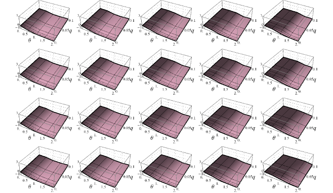
(a) Grid of 3D bias surfaces for $\hat{D}_{\mathrm{uj1}}$.

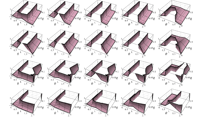
(b) Grid of 3D bias surfaces for $\hat{D}_{\mathrm{uj2}}$.

Figure 1: Notice that $\hat{D}_{\mathrm{uj1}}$ is a consistent under-estimator of distinct values. Although second order, $\hat{D}_{\mathrm{uj2}}$ has considerably worse and irregular bias behavior as compared to $\hat{D}_{\mathrm{uj1}}$. Recall that the layout of the surfaces is on the grid indicated by Table 2.

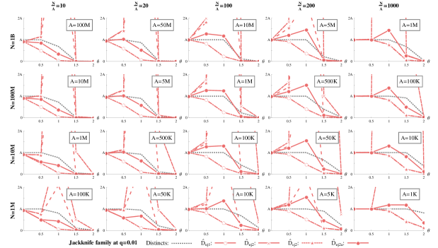
(a)

Figure 2: Relative behavior of the jackknife family at $q=0.01$, which is the lowest $q$ at which $\hat{D}_{\mathrm{uj2a}}$ has a maximum error-ratio of 5 (see Table 6). Note the consistent underestimation of $\hat{D}_{\mathrm{uj1}}$, severe mid-skew biases of $\hat{D}_{\mathrm{uj2}}$ and $\hat{D}_{\mathrm{sj2}}$, and effect of stabilization in $\hat{D}_{\mathrm{uj2a}}$.

Variation with $\frac{N}{A}$:

$\hat{D}_{\mathrm{uj1}}$ is fairly agnostic to changes in $\frac{N}{A}$, at all values of $q$. On the other hand, the positive bias of $\hat{D}_{\mathrm{uj2}}$ shoots up as $\frac{N}{A}$ increases. The magnitude of the positive bias is highest at mid-skew.

For $\hat{D}_{\mathrm{sj2}}$, the bias 3D surface illustrates best the severe positive bias at mid-skew. Importantly, the bias magnitude, as also the region, reduces as $\frac{N}{A}$ increases. In other words, smoothing is more effective as $\frac{N}{A}$ increases. At $\frac{N}{A}=10$, we need considerably over 10% sampling to get accurate estimates. As $\frac{N}{A}$ increases, the least sampling fraction $q$ required to get accurate estimates reduces.

The stabilized estimator $\hat{D}_{\mathrm{uj2a}}$ is quite accurate overall. There is a jump between low and high skew estimates that increases with $\frac{N}{A}$ when $q<0.05$. There is a bump at mid-skew for low $q$ and high $\frac{N}{A}$; it flattens out at lower $\frac{N}{A}$.

Variation with $N$ keeping $\frac{N}{A}$ fixed:

$\hat{D}_{\mathrm{uj1}}$ is fairly agnostic of $N$. On the other hand, the accuracy of $\hat{D}_{\mathrm{uj2}}$ at high skew varies with $N$: $\hat{D}_{\mathrm{uj2}}$ is more accurate at high skew at high $N$, and inaccurate at low $N$. $\hat{D}_{\mathrm{sj2}}$ is slightly worse at mid-skew as $N$ increases. Finally, $\hat{D}_{\mathrm{uj2a}}$ is fairly agnostic to $N$.

Variation with $\theta$:

As is known [3], $\hat{D}_{\mathrm{uj1}}$ is a consistent underestimator across all $\theta$. We observe that the negative bias is the worst at mid-high skew. The bias profile of $\hat{D}_{\mathrm{uj2}}$ is best described as “hat-shaped”. There is severe positive bias at mid-skew. There is slight positive bias at low-skew, and moderate to high positive bias at high-skew up to $N=100M$. At $N>100M$, $\hat{D}_{\mathrm{uj2}}$ becomes an underestimator at high-skew. The positive bias at high-skew for low $N$ gets worse as we increase $q$. $\hat{D}_{\mathrm{sj2}}$ shows the same pattern of positive bias as $\hat{D}_{\mathrm{uj2}}$, but less prominently owing to the smoothing. Smoothing also delays the poor performance at high $\frac{N}{A}$.

$\hat{D}_{\mathrm{uj2a}}$ has a crossover in the form of a reflected “S” shape as we increase skew. In other words, it overestimates at mid skew and underestimates at high skew. See also Fig. 8. At high $\frac{N}{A}$, the bias goes from positive to negative as skew increases, whereas at low $\frac{N}{A}$, it remains largely positive, with some overestimation at high $q$.

empty

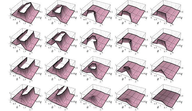
(a) Grid of 3D bias surfaces for $\hat{D}_{\mathrm{sj2}}$

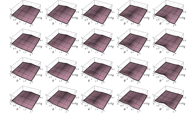
(b) Grid of 3D bias surfaces for $\hat{D}_{\mathrm{uj2a}}$

Figure 3: Effect of smoothing versus stabilization can be seen clearly: the stabilized $\hat{D}_{\mathrm{uj2a}}$ is one of the most consistently accurate estimators, while the smoothed $\hat{D}_{\mathrm{sj2}}$ is suffers severe mid-skew bias at low $\frac{N}{A}$. Note the effect of $\frac{N}{A}$ versus that of $N$ in $\hat{D}_{\mathrm{sj2}}$.

Variation with $q$:

As we might expect, $\hat{D}_{\mathrm{uj1}}$ reduces its negative bias as $q$ increases. $\hat{D}_{\mathrm{uj2}}$, at high $\frac{N}{A}$, improves dramatically in mid-skew as $q$ increases above 5%. Whereas, at low $\frac{N}{A}$, increasing $q$ does not help.

For $\hat{D}_{\mathrm{sj2}}$ increasing $q$ helps more at high $\frac{N}{A}$ (100 or greater). For $\frac{N}{A}=100$, we need $q>10\%$, for $\frac{N}{A}=200$ this drops to $q>5\%$, and for $\frac{N}{A}=1000$, we need only $q>1\%$ for acceptable estimates. $\hat{D}_{\mathrm{uj2a}}$ does well at all sampling fractions and improves accuracy with $q$. At high Zipfian skew of $\theta\geq 1.5$, we need only $q\geq 0.005$ for accurate estimates.

Anomalies:

The bias of $\hat{D}_{\mathrm{uj2}}$ is lower at $q=0.001$ as compared to higher values of $q$ in the vicinity. The smoothing technique of $\hat{D}_{\mathrm{sj2}}$ does well at low $\frac{N}{A}\sim 10$, and very low sampling ($q$ = 0.001), but then exhibits poor performance as either of these parameters increases.

4.2 The Schlosser Estimators

empty

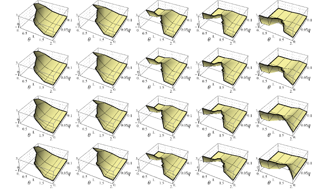
(a) Grid of 3D bias surfaces for $\hat{D}_{\mathrm{Sh}}$

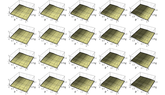
(b) Grid of 3D bias surfaces for $\hat{D}_{\mathrm{Sh2}}$

Figure 4: $\hat{D}_{\mathrm{Sh}}$ shows severe positive bias at lower skew, that is corrected only with high sampling fractions. $\hat{D}_{\mathrm{Sh2}}$ does not suffer from this problem. Note the highly regular behavior of both, especially clear with $\hat{D}_{\mathrm{Sh}}$, as a function of $\frac{N}{A}$ alone.

Bias:

The Schlossers have the general bias profile $\hat{D}_{\mathrm{Sh}}>\hat{D}_{\mathrm{Sh3}}>D>\hat{D}_{\mathrm{Sh2}}$: the exception being at low $\frac{N}{A}$ and low $q$ where $\hat{D}_{\mathrm{Sh}}$ and $\hat{D}_{\mathrm{Sh3}}$ underestimate, but only slightly.

Variation with $\frac{N}{A}$:

For $\hat{D}_{\mathrm{Sh}}$ and $\hat{D}_{\mathrm{Sh3}}$, the bias curve is a slope at lower $\frac{N}{A}$ and becomes a “hat” at higher $\frac{N}{A}$. The value of $\frac{N}{A}$ at which this shape transition happens reduces as $q$ increases. For $q=0.001$, it happens after $\frac{N}{A}>1000$, at $q=0.005$, it happens for $\frac{N}{A}$ between 1000 and 200, and for $q=0.02$, it occurs for $\frac{N}{A}$ between 200 and 100. Increase in $q$ improves accuracy as $\frac{N}{A}$ increases, with this improvement manifesting at low skewness.

$\hat{D}_{\mathrm{Sh3}}$ is reasonably accurate at $q\geq 0.005$. $\hat{D}_{\mathrm{Sh}}$ requires $q\geq 0.01$ for acceptable estimates. As $q$ increases, the $\frac{N}{A}$ at which the accuracy is attained for low skew reduces, and the range of low-skew where the accuracy is attained also increases. For low $\frac{N}{A}\sim 10$, low skew estimates remain intolerably poor until we raise the sampling fraction to $q=0.1$.

The predominant effect of increasing $\frac{N}{A}$ on all three is that the lower skew estimate becomes reasonably accurate. See also Fig. 8 for this effect in $\hat{D}_{\mathrm{Sh2}}$.

Variation with $N$:

There is little change in the shape of the bias surfaces as we increase $N$, keeping $\frac{N}{A}$ fixed.

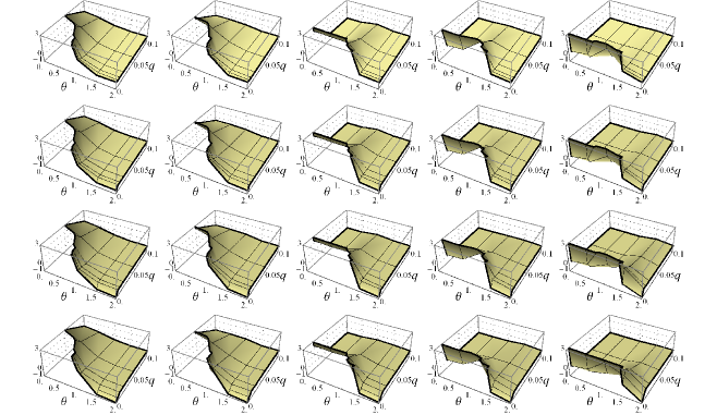
Figure 5: Grid of 3D bias surface for $\hat{D}_{\mathrm{Sh3}}$. Like $\hat{D}_{\mathrm{Sh}}$, there is severe positive bias at low skew. Note again the highly regular behavior of $\hat{D}_{\mathrm{Sh3}}$ as a function of $\frac{N}{A}$ alone.

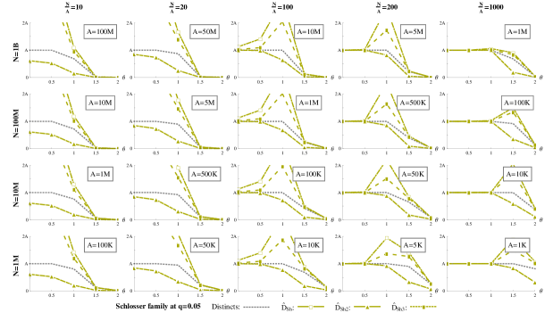
(a)

Figure 6: Relative behavior of the Schlosser family at $q=0.05$, which is the lowest $q$ at which $\hat{D}_{\mathrm{Sh2}}$ has a maximum ratio-error of 5. Even at a relatively high sampling fraction, $\hat{D}_{\mathrm{Sh}}$ and $\hat{D}_{\mathrm{Sh3}}$ show severe positive bias at low-mid skew. In order to use these estimators at low-mid skew, $q\geq 0.1$ is required.

Variation with $\theta$:

$\hat{D}_{\mathrm{Sh}}$ and $\hat{D}_{\mathrm{Sh3}}$ are extremely accurate for high-skew. When the bias curve becomes a hat, as described earlier, the estimator is accurate at low skew also (pl. see variation with $\frac{N}{A}$ for discussion of when it becomes a hat). When this happens, only mid-skew is overestimated. $\hat{D}_{\mathrm{Sh2}}$ has a negative bias at low-mid skew, but is not as extreme as $\hat{D}_{\mathrm{Sh}}$ and $\hat{D}_{\mathrm{Sh3}}$.

Variation with $q$:

This family is very sensitive to $q$, and shows monotonic improvement in accuracy (which means lesser positive bias) as $q$ increases. In the range of 5 - 10% sampling, all three estimators begin giving accurate estimates for all $\frac{N}{A}$, all skew, and all $N$, giving a maximum ratio error of $\sim 5$. Of these, $\hat{D}_{\mathrm{Sh3}}$ is requires the lowest $q$ to provide acceptable estimates across the range of skew (see Table 6.

4.3 $\hat{D}_{\mathrm{GEE}}$ and $\hat{D}_{\mathrm{AE}}$

empty

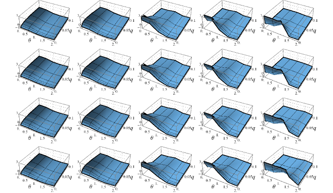
(a) Grid of 3D bias surface for $\hat{D}_{\mathrm{GEE}}$

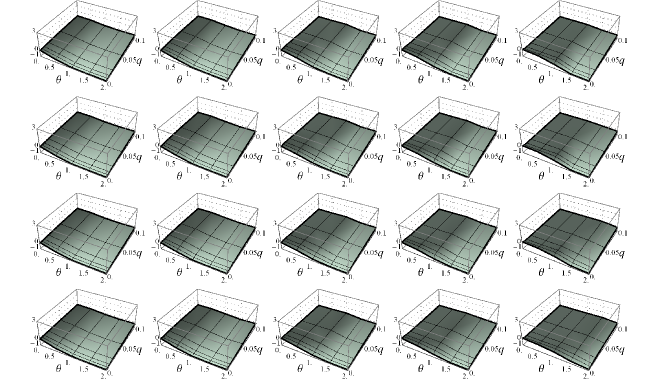
(b) Grid of 3D bias surface for $\hat{D}_{\mathrm{AE}}$

Figure 7: $\hat{D}_{\mathrm{GEE}}$ and $\hat{D}_{\mathrm{AE}}$ are among the most consistent estimators. $\hat{D}_{\mathrm{GEE}}$ does have a region of positive bias at high $\frac{N}{A}$, where it should not be used in preference to $\hat{D}_{\mathrm{AE}}$ and $\hat{D}_{\mathrm{uj2a}}$. Both estimators show highly regular behavior as a function of $\frac{N}{A}$.

Variation with $\frac{N}{A}$:

At low $\frac{N}{A}\sim 10$, both $\hat{D}_{\mathrm{GEE}}$ and $\hat{D}_{\mathrm{AE}}$ underestimate but both are reasonably accurate. As we increase $\frac{N}{A}$, this picture changes significantly for $\hat{D}_{\mathrm{GEE}}$, but not for $\hat{D}_{\mathrm{AE}}$ (see Fig. 7. $\hat{D}_{\mathrm{AE}}$ shows considerably less change w.r.t. $\frac{N}{A}$. The change of $\hat{D}_{\mathrm{GEE}}$ with $\frac{N}{A}$ is described next. There is a change from a slope to a “hat”, similar to $\hat{D}_{\mathrm{Sh}}$ and $\hat{D}_{\mathrm{Sh3}}$, as $\frac{N}{A}$ rises. However, the degree of overestimation is not comparable the Schlossers. The ratio errors for the worst case positive bias is less than 10, compared to over 200 for Schlossers. The transition to “hat” happens at $q=0.005$ at $\frac{N}{A}$ between 1000 and 200; at $q=0.02$ between 200 and 100; and at $q=0.1$ between 100 and 20.

Variation with $N$:

There is little change with $N$ except for some reduction in positive bias for high-skew for $\hat{D}_{\mathrm{GEE}}$ with $N$.

Variation with $\theta$:

$\hat{D}_{\mathrm{GEE}}$ is very good at high skew. When the transition to “hat” shape happens, it becomes good at low skew as well (see previous discussion of when this happens). $\hat{D}_{\mathrm{GEE}}$ is a mid-skew overestimator (except at very low $q$, where it underestimates). $\hat{D}_{\mathrm{AE}}$ is accurate at both high and low skew Zipfian populations, with a tendency towards negative bias. See also Fig. 8.

Since both $\hat{D}_{\mathrm{GEE}}$ and $\hat{D}_{\mathrm{AE}}$ appear in the grid of 2D bias plots for the top three estimators in Sec 5, we do not show their 2D bias plots here. Of course, all the 2D bias plots are available in the supplementaries.

Variation with $q$:

Both estimators show monotonic improvement in accuracy (reduction in positive bias) for increase in $q$. For $\hat{D}_{\mathrm{GEE}}$, at $q=0.005$ worst case ratio error is 5, at $q=0.01$, it drops to 4, at $q=0.05$, it is less than 2.

Anomalies:

When changing $\frac{N}{A}$ from 20 to 100, there is a sudden increase in $\hat{D}_{\mathrm{GEE}}$ positive bias up to $q=0.01$.

empty

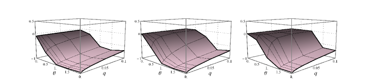
(a) $\hat{D}_{\mathrm{uj1}}$

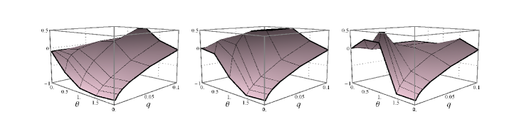
(b) $\hat{D}_{\mathrm{uj2a}}$

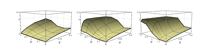
(c) $\hat{D}_{\mathrm{Sh2}}$

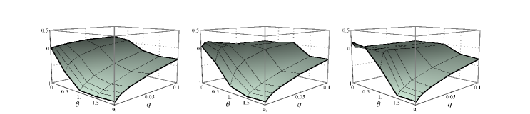
(d) $\hat{D}_{\mathrm{AE}}$

Figure 8: The “flatter” bias surfaces of $\hat{D}_{\mathrm{uj1}}$, $\hat{D}_{\mathrm{uj2a}}$, $\hat{D}_{\mathrm{Sh2}}$, and $\hat{D}_{\mathrm{AE}}$ shown with more detail. Only $N=1B$, and $\frac{N}{A}\in[10,100,1000]$ shown. Note also that these estimators are relatively agnostic to $N$, and show regularity in variation with $\frac{N}{A}$.

4.4 The Chao-Lee Estimators

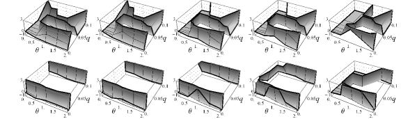
Figure 9: The two Chao-Lee estimators show highly irregular behavior that becomes extreme even at $N=10M$. Therefore we show only 1M and 10M population sizes for $\hat{D}_{\mathrm{CL2}}$. The remaining 3D surfaces for $\hat{D}_{\mathrm{CL2}}$ are available in supplementaries.

The Chao-Lee estimators show highly erratic behavior, and perform reasonably only in following regions.

At $q$ =0.001, $N$ =1M, 10M

At $q$ =0.005, $N$ =10M

At $q$ =0.001, $N$ =100M

At $q$ =0.5, $N$ =1M and 100M

At $q$ =0.1, $N$ =10M

The variations described below only pertain to the above regions.
Variation with $\frac{N}{A}$: Not much change except at q = 0.001.
Variation with $N$: Discontinuity is the predominant effect.
Variation with $\theta$ and $q$: When $q>0.005$, both underestimate in mid-high skew.

5 Discussion

The discussion is organized as follows. First we describe the relative sensitivity of each estimator to the various parameters. Then we address the question “which are the best estimators?” in terms of accuracy over the entire parameter space of our characterization. Next, we identify regions of the parameter space where certain estimators do well, even though they may not perform well over the entire parameter space. Finally, we address the question “how much sampling do we need?”

5.1 Sensitivity to Parameters

Sensitivity to $\frac{N}{A}$:

The grids of 3D bias surfaces clearly show that every family — the Schlossers, jackknives, $\hat{D}_{\mathrm{GEE}}$ and $\hat{D}_{\mathrm{AE}}$, and Chao-Lee — is sensitive to changes in $\frac{N}{A}$, and all except the last show regularity in their behaviour as a function of $\frac{N}{A}$. The parameter $\frac{N}{A}$ emerges as the single most important organizing parameter for estimator behavior overall. The sensitivity to $\frac{N}{A}$ is high in $\hat{D}_{\mathrm{Sh}}$, $\hat{D}_{\mathrm{Sh3}}$, $\hat{D}_{\mathrm{uj2}}$, $\hat{D}_{\mathrm{sj2}}$, $\hat{D}_{\mathrm{GEE}}$, $\hat{D}_{\mathrm{CL1}}$, and $\hat{D}_{\mathrm{CL2}}$. Compared to the above, there was mild sensitivity in $\hat{D}_{\mathrm{uj1}}$, $\hat{D}_{\mathrm{uj2a}}$, $\hat{D}_{\mathrm{Sh2}}$, and $\hat{D}_{\mathrm{AE}}$. Therefore, even within a family, some members are highly sensitive to changes in $\frac{N}{A}$, while others are not.

Sensitivity to Scale $N$:

Among the 11 estimators we tested, $\hat{D}_{\mathrm{sj2}}$, and the two Chao-Lee estimators were highly sensitive to scale. Namely, as we go up vertically along their grids, their 3D bias surfaces showed significant changes. Of these, the change was quite regular and predictable in $\hat{D}_{\mathrm{sj2}}$, but irregular and unpredictable in the Chao-Lee families. In the case of $\hat{D}_{\mathrm{sj2}}$, the bias increases as we increase the scale, with the increase being most prominent around mid-skew as can be seen from the 3D bias surfaces for $\hat{D}_{\mathrm{sj2}}$ (Fig 3a). See supplementaries for complete Chao-Lee estimator grids.

Sensitivity to Sampling Fraction $q$:

The 2D plots (see supplementaries) are useful to illustrate the effect of sampling fraction. The estimators that improve most as $q$ increases are $\hat{D}_{\mathrm{Sh}}$, $\hat{D}_{\mathrm{Sh3}}$, $\hat{D}_{\mathrm{GEE}}$. The estimators that are relatively less sensitive to increases in $q$ in our range, for some values of other parameters, are $\hat{D}_{\mathrm{uj2a}}$ and $\hat{D}_{\mathrm{AE}}$. For example, both of them remain relatively accurate for low skew even at low sampling fractions (see Tables 3b and 4b).

The estimators that show anomalous or irregular behavior as $q$ is increased are $\hat{D}_{\mathrm{uj2}}$, $\hat{D}_{\mathrm{sj2}}$, and the Chao-Lee family. In the case of $\hat{D}_{\mathrm{uj2}}$ and $\hat{D}_{\mathrm{sj2}}$, we see anomalous degradation in performance as we go from $q$ = 0.001 to 0.005, especially when $\frac{N}{A}<200$, see 2D plots in supplementaries.

Sensitivity to Zifpian Skew $\theta$:

Sensitivity to $\theta$ can be seen more finely in the 2D plots (see supplementaries). The estimators $\hat{D}_{\mathrm{Sh}}$, $\hat{D}_{\mathrm{Sh3}}$, $\hat{D}_{\mathrm{uj2}}$, $\hat{D}_{\mathrm{sj2}}$, and $\hat{D}_{\mathrm{GEE}}$ are highly sensitive to changes in Zipfian skew. In particular, $\hat{D}_{\mathrm{Sh}}$ and $\hat{D}_{\mathrm{Sh3}}$ are quite inaccurate at low skew. $\hat{D}_{\mathrm{uj2}}$ and $\hat{D}_{\mathrm{sj2}}$ perform poorly in mid-skew, while $\hat{D}_{\mathrm{uj2}}$ also performs poorly for smaller populations and high skew, even at high sampling fractions.

The estimators $\hat{D}_{\mathrm{Sh2}}$, $\hat{D}_{\mathrm{uj1}}$, $\hat{D}_{\mathrm{uj2a}}$, and $\hat{D}_{\mathrm{AE}}$ are relatively insensitive to changes in Zipfian skew. Finally, $\hat{D}_{\mathrm{CL1}}$ and $\hat{D}_{\mathrm{CL2}}$ respond irregularly to changes in Zifpian skew.

5.2 The Best Estimators Overall and their Relative Performance

From our extensive study, we can conclude that three estimators provide relatively strong performance across variations in all underlying parameters. These three are $\hat{D}_{\mathrm{GEE}}$, $\hat{D}_{\mathrm{AE}}$, and $\hat{D}_{\mathrm{uj2a}}$ (cf. the choice of the provisional estimator in [3], which is $\hat{D}_{\mathrm{sj2}}$). It is perhaps easiest to see this from Table 3b, and inspect the low and high sampling cases separately. Of course, which estimator is to be used for an application depends on the sampling fraction that is available (we return to this question in $\S.~{}\ref{sec:sampling-fraction})$, and the skewness of the population in case it is known. A subtler issue is whether it is the ratio error that is critical to the application, or the actual value and sign of the bias, and the role played by $\frac{N}{A}$. For example, when the number of distincts is relatively low, even large ratio errors do not result in high absolute value of bias. Therefore, we cannot speak meaningfully about “best estimator” in terms of just ratio error or bias — we do need to include the $\frac{N}{A}$ factor as well. Since in certain database query optimizers, it may be the value and sign of bias that is the critical factor in change of a query plan, while in others, it may be the ratio error, practitioners will find it useful to have an analysis along both metrics. In both cases, we discuss the low sampling scenario ($q<0.01$) below since that is where differences may be most manifest.

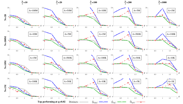
(a)

Figure 10: The three most consistent estimators at $q=0.02$, which is the lowest $q$ at which $\hat{D}_{\mathrm{AE}}$ has maximum ratio error at most 5, see Table 6 (although $\hat{D}_{\mathrm{uj2a}}$ offers the same at $q=0.01$). Note that at mid-high $\frac{N}{A}$ there is a region of significant low-mid skew bias for $\hat{D}_{\mathrm{GEE}}$, described in text.

Table 3: Ratio-error vs. $\theta$ and $\frac{N}{A}$, for low and high sampling fractions. Note that the high and low ranges for $\frac{N}{A}$ overlap on the mid-value of $\frac{N}{A}=100$.

$\begin{array}[]{|cc|cccc|cccc|}\hline\cr&&\lx@intercol\hfil\text{$0.001\leq q\leq 0.005$}\hfil\lx@intercol\vrule\lx@intercol&\lx@intercol\hfil\text{$0.01\leq q\leq 0.1$}\hfil\lx@intercol\vrule\lx@intercol\\ \cline{3-10}\cr\text{Skew}&\text{$\frac{N}{A}$}&\text{$\hat{D}_{\mathrm{uj1}}$}&\text{$\hat{D}_{\mathrm{uj2}}$}&\text{$\hat{D}_{\mathrm{sj2}}$}&\text{$\hat{D}_{\mathrm{uj2a}}$}&\text{$\hat{D}_{\mathrm{uj1}}$}&\text{$\hat{D}_{\mathrm{uj2}}$}&\text{$\hat{D}_{\mathrm{sj2}}$}&\text{$\hat{D}_{\mathrm{uj2a}}$}\bigstrut[t]\bigstrut[b]\\ \hline\cr 0\leq\theta\leq 1&\frac{N}{A}\leq 100&12.99&8.24&3.33&2.43&2.69&28.23&4.16&1.23\bigstrut[t]\\ 1.5\leq\theta\leq 2&\frac{N}{A}\leq 100&38.56&5.8&38.69&9.24&8.06&8.88&8.14&2.07\\ 0\leq\theta\leq 1&\frac{N}{A}\geq 100&3.04&19.89&3.46&1.28&1.22&19.26&1.63&1.13\\ 1.5\leq\theta\leq 2&\frac{N}{A}\geq 100&27.8&6.57&28.5&7.21&6.23&9.46&6.27&1.83\bigstrut[b]\\ \hline\cr\end{array}$

(a)

$\begin{array}[]{|cc|ccc|cc|ccc|cc|}\hline\cr&&\lx@intercol\hfil\text{$0.001\leq q\leq 0.005$}\hfil\lx@intercol\vrule\lx@intercol&\lx@intercol\hfil\text{$0.01\leq q\leq 0.1$}\hfil\lx@intercol\vrule\lx@intercol\\ \cline{3-12}\cr\text{Skew}&\text{$\frac{N}{A}$}&\text{$\hat{D}_{\mathrm{Sh}}$}&\text{$\hat{D}_{\mathrm{Sh2}}$}&\text{$\hat{D}_{\mathrm{Sh3}}$}&\text{$\hat{D}_{\mathrm{GEE}}$}&\text{$\hat{D}_{\mathrm{AE}}$}&\text{$\hat{D}_{\mathrm{Sh}}$}&\text{$\hat{D}_{\mathrm{Sh2}}$}&\text{$\hat{D}_{\mathrm{Sh3}}$}&\text{$\hat{D}_{\mathrm{GEE}}$}&\text{$\hat{D}_{\mathrm{AE}}$}\bigstrut[t]\bigstrut[b]\\ \hline\cr 0\leq\theta\leq 1&\frac{N}{A}\leq 100&19.39&25.57&16.96&2.49&4.17&5.41&3.11&4.18&1.62&1.41\bigstrut[t]\\ 1.5\leq\theta\leq 2&\frac{N}{A}\leq 100&1.15&36.32&2.53&2.69&14.29&1.07&6.86&1.06&1.93&3.09\\ 0\leq\theta\leq 1&\frac{N}{A}\geq 100&64.7&3.87&45.7&4.27&1.56&4.08&1.2&2.57&1.65&1.06\\ 1.5\leq\theta\leq 2&\frac{N}{A}\geq 100&1.81&26.19&2.23&2.12&10.94&1.32&5.39&1.23&1.65&2.62\bigstrut[b]\\ \hline\cr\end{array}$

(b)

Table 4: Percentage bias vs. $\theta$ and $\frac{N}{A}$ for low and high sampling fractions. Shaded cells indicate a change in the sign of the bias in the individual values within that region.

$\begin{array}[]{|cc|cccc|cccc|}\hline\cr&&\lx@intercol\hfil\text{$0.001\leq q\leq 0.005$}\hfil\lx@intercol\vrule\lx@intercol&\lx@intercol\hfil\text{$0.01\leq q\leq 0.1$}\hfil\lx@intercol\vrule\lx@intercol\\ \cline{3-10}\cr\text{Skew}&\text{$\frac{N}{A}$}&\text{$\hat{D}_{\mathrm{uj1}}$}&\text{$\hat{D}_{\mathrm{uj2}}$}&\text{$\hat{D}_{\mathrm{sj2}}$}&\text{$\hat{D}_{\mathrm{uj2a}}$}&\text{$\hat{D}_{\mathrm{uj1}}$}&\text{$\hat{D}_{\mathrm{uj2}}$}&\text{$\hat{D}_{\mathrm{sj2}}$}&\text{$\hat{D}_{\mathrm{uj2a}}$}\bigstrut[t]\bigstrut[b]\\ \hline\cr 0\leq\theta\leq 1&\frac{N}{A}\leq 100&\pagecolor[gray]{0.8}{-50.01}&\pagecolor[gray]{0.8}{680.77}&\pagecolor[gray]{0.8}{181.94}&\pagecolor[gray]{0.8}{-34.67}&\pagecolor[gray]{0.8}{-33.07}&\pagecolor[gray]{0.8}{2,719.94}&\pagecolor[gray]{0.8}{310.84}&\pagecolor[gray]{0.8}{6.31}\bigstrut[t]\\ 1.5\leq\theta\leq 2&\frac{N}{A}\leq 100&-96.19&\pagecolor[gray]{0.8}{68.14}&-96.22&-86.06&-83.27&\pagecolor[gray]{0.8}{610.59}&-83.36&\pagecolor[gray]{0.8}{-37.33}\\ 0\leq\theta\leq 1&\frac{N}{A}\geq 100&\pagecolor[gray]{0.8}{-32.34}&\pagecolor[gray]{0.8}{1,886.06}&\pagecolor[gray]{0.8}{241.56}&\pagecolor[gray]{0.8}{1.38}&\pagecolor[gray]{0.8}{-10.24}&\pagecolor[gray]{0.8}{1,825.79}&\pagecolor[gray]{0.8}{57.9}&\pagecolor[gray]{0.8}{12.77}\\ 1.5\leq\theta\leq 2&\frac{N}{A}\geq 100&-94.36&\pagecolor[gray]{0.8}{159.33}&-94.41&\pagecolor[gray]{0.8}{-79.67}&-77.14&\pagecolor[gray]{0.8}{661.2}&-77.24&\pagecolor[gray]{0.8}{-28.31}\bigstrut[b]\\ \hline\cr\end{array}$

(a)

$\begin{array}[]{|cc|ccc|cc|ccc|cc|}\hline\cr&&\lx@intercol\hfil\text{$0.001\leq q\leq 0.005$}\hfil\lx@intercol\vrule\lx@intercol&\lx@intercol\hfil\text{$0.01\leq q\leq 0.1$}\hfil\lx@intercol\vrule\lx@intercol\\ \cline{3-12}\cr\text{Skew}&\text{$\frac{N}{A}$}&\text{$\hat{D}_{\mathrm{Sh}}$}&\text{$\hat{D}_{\mathrm{Sh2}}$}&\text{$\hat{D}_{\mathrm{Sh3}}$}&\text{$\hat{D}_{\mathrm{GEE}}$}&\text{$\hat{D}_{\mathrm{AE}}$}&\text{$\hat{D}_{\mathrm{Sh}}$}&\text{$\hat{D}_{\mathrm{Sh2}}$}&\text{$\hat{D}_{\mathrm{Sh3}}$}&\text{$\hat{D}_{\mathrm{GEE}}$}&\text{$\hat{D}_{\mathrm{AE}}$}\bigstrut[t]\bigstrut[b]\\ \hline\cr 0\leq\theta\leq 1&\frac{N}{A}\leq 100&\text{1,839.04}&-87.59&\text{1,596.3}&\pagecolor[gray]{0.8}{13.26}&\pagecolor[gray]{0.8}{-38.34}&441.38&\pagecolor[gray]{0.8}{-46.03}&\pagecolor[gray]{0.8}{318.15}&\pagecolor[gray]{0.8}{35.78}&\pagecolor[gray]{0.8}{-10.28}\bigstrut[t]\\ 1.5\leq\theta\leq 2&\frac{N}{A}\leq 100&\pagecolor[gray]{0.8}{10.14}&-95.93&\pagecolor[gray]{0.8}{-31.19}&-58.5&-90.66&\pagecolor[gray]{0.8}{5.12}&-79.94&\pagecolor[gray]{0.8}{3.59}&-46.19&-58.73\\ 0\leq\theta\leq 1&\frac{N}{A}\geq 100&\text{6,370.46}&\pagecolor[gray]{0.8}{-49.79}&\text{4,470.08}&\pagecolor[gray]{0.8}{326.4}&\pagecolor[gray]{0.8}{-13.12}&\pagecolor[gray]{0.8}{307.72}&\pagecolor[gray]{0.8}{-9.85}&\pagecolor[gray]{0.8}{156.69}&\pagecolor[gray]{0.8}{64.86}&\pagecolor[gray]{0.8}{0.89}\\ 1.5\leq\theta\leq 2&\frac{N}{A}\geq 100&\pagecolor[gray]{0.8}{76.9}&-93.98&\pagecolor[gray]{0.8}{-3.22}&\pagecolor[gray]{0.8}{-38.63}&-86.62&\pagecolor[gray]{0.8}{30.47}&-73.45&\pagecolor[gray]{0.8}{21.91}&\pagecolor[gray]{0.8}{-29.78}&\pagecolor[gray]{0.8}{-51.53}\bigstrut[b]\\ \hline\cr\end{array}$

(b)

Table 5: Percentage RMSE vs. $\gamma^{2}$ and $\frac{N}{A}$ for low and high sampling fractions

$\begin{array}[]{|cc|cccc|cccc|}\hline\cr&&\lx@intercol\hfil\text{$0.001\leq q\leq 0.005$}\hfil\lx@intercol\vrule\lx@intercol&\lx@intercol\hfil\text{$0.01\leq q\leq 0.1$}\hfil\lx@intercol\vrule\lx@intercol\\ \cline{3-10}\cr\text{$\gamma^{2}$}&\text{$\frac{N}{A}$}&\text{$\hat{D}_{\mathrm{uj1}}$}&\text{$\hat{D}_{\mathrm{uj2}}$}&\text{$\hat{D}_{\mathrm{sj2}}$}&\text{$\hat{D}_{\mathrm{uj2a}}$}&\text{$\hat{D}_{\mathrm{uj1}}$}&\text{$\hat{D}_{\mathrm{uj2}}$}&\text{$\hat{D}_{\mathrm{sj2}}$}&\text{$\hat{D}_{\mathrm{uj2a}}$}\bigstrut[t]\bigstrut[b]\\ \hline\cr 0\leq\gamma^{2}<1&\frac{N}{A}\leq 100&63.68&\text{2,293.07}&575.77&48.91&45.78&\text{5,816.36}&705.15&26.77\bigstrut[t]\\ 1\leq\gamma^{2}\leq 50&\frac{N}{A}\leq 100&96.21&228.61&96.24&86.3&83.7&\text{1,571.14}&83.79&47.92\\ \gamma^{2}>50&\frac{N}{A}\leq 100&95.63&\text{2,300.52}&580.57&80.51&80.49&\text{5,956.07}&708.07&45.69\\ 0\leq\gamma^{2}<1&\frac{N}{A}\geq 100&46.63&\text{4,998.23}&627.08&28.2&21.49&\text{4,528.98}&230.89&23.17\\ 1\leq\gamma^{2}\leq 50&\frac{N}{A}\geq 100&94.48&467.77&94.52&81.3&78.61&\text{1,577.23}&78.7&43.14\\ \gamma^{2}>50&\frac{N}{A}\geq 100&89.48&\text{5,083.31}&640.39&70.98&68.54&\text{4,775.1}&242.68&42.17\bigstrut[b]\\ \hline\cr\end{array}$

(a)

$\begin{array}[]{|cc|ccc|cc|ccc|cc|}\hline\cr&&\lx@intercol\hfil\text{$0.001\leq q\leq 0.005$}\hfil\lx@intercol\vrule\lx@intercol&\lx@intercol\hfil\text{$0.01\leq q\leq 0.1$}\hfil\lx@intercol\vrule\lx@intercol\\ \cline{3-12}\cr\text{$\gamma^{2}$}&\text{$\frac{N}{A}$}&\text{$\hat{D}_{\mathrm{Sh}}$}&\text{$\hat{D}_{\mathrm{Sh2}}$}&\text{$\hat{D}_{\mathrm{Sh3}}$}&\text{$\hat{D}_{\mathrm{GEE}}$}&\text{$\hat{D}_{\mathrm{AE}}$}&\text{$\hat{D}_{\mathrm{Sh}}$}&\text{$\hat{D}_{\mathrm{Sh2}}$}&\text{$\hat{D}_{\mathrm{Sh3}}$}&\text{$\hat{D}_{\mathrm{GEE}}$}&\text{$\hat{D}_{\mathrm{AE}}$}\bigstrut[t]\bigstrut[b]\\ \hline\cr 0\leq\gamma^{2}<1&\frac{N}{A}\leq 100&\text{2,856.32}&88.96&\text{2,563.94}&115.98&55.95&653.14&55.16&478.76&79.1&28.25\bigstrut[t]\\ 1\leq\gamma^{2}\leq 50&\frac{N}{A}\leq 100&23.05&95.96&47.43&59.92&90.77&11.04&80.63&9.46&47.21&61.86\\ \gamma^{2}>50&\frac{N}{A}\leq 100&403.1&95.5&218.4&60.89&88.46&131.95&77.48&80.6&46.66&56.92\\ 0\leq\gamma^{2}<1&\frac{N}{A}\geq 100&\text{9,061.75}&58.72&\text{6,462.05}&433.9&32.17&610.17&20.07&339.7&106.91&8.92\\ 1\leq\gamma^{2}\leq 50&\frac{N}{A}\geq 100&185.16&94.12&62.61&57.05&87.24&64.65&75.33&45.18&41.94&56.27\\ \gamma^{2}>50&\frac{N}{A}\geq 100&\text{1,434.17}&89.1&636.45&130.03&78.32&224.9&65.37&124.14&61.5&47.23\bigstrut[b]\\ \hline\cr\end{array}$

(b)

5.2.1 By Ratio Error

See Table 3b. For low sampling fractions, for low $\frac{N}{A}$, $\hat{D}_{\mathrm{uj2a}}$ and $\hat{D}_{\mathrm{GEE}}$ are the best estimators when $0\leq\theta\leq 1$. For higher skew, only $\hat{D}_{\mathrm{GEE}}$ continues to perform well. At high $\frac{N}{A}$, and low-mid skew, $\hat{D}_{\mathrm{uj2a}}$ and $\hat{D}_{\mathrm{AE}}$ are the best, which $\hat{D}_{\mathrm{GEE}}$ again does very well as $\frac{N}{A}$ increases.

Caveat: If $\frac{N}{A}$ is mid-high, and the data has low-mid skew, then $\hat{D}_{\mathrm{GEE}}$ should not be used unless the sampling fraction is greater than 0.01.

5.2.2 By Bias

See Table 4b. For low sampling fractions and for low $\frac{N}{A}$, all three — $\hat{D}_{\mathrm{uj2a}}$, $\hat{D}_{\mathrm{GEE}}$, $\hat{D}_{\mathrm{AE}}$— do well measured by bias. For high $\frac{N}{A}$, for low-mid skew, $\hat{D}_{\mathrm{uj2a}}$ and $\hat{D}_{\mathrm{AE}}$ are the best estimators. As we raise skew, $\hat{D}_{\mathrm{GEE}}$ is more accurate than both; however, all three are good.

Note that by either metric — bias or ratio error — the provisional choice $\hat{D}_{\mathrm{CL2}}$ estimator given in [3] is poor.

5.3 Regions of Good Performance

The three estimators discussed above do reasonably well in all regions. However, there are other estimators that actually do better than these, but in small sub-domains. However, these sub-domains are clearly delineated, and therefore we can potentially use these estimators when our data lies in the corresponding domains.

5.3.1 Regions Defined by Zipfian Skew

The best example of such estimators are $\hat{D}_{\mathrm{Sh}}$ and $\hat{D}_{\mathrm{Sh3}}$. Whether sampling fractions are low or high, these estimators absolutely shine in the high skew region of $\theta>1.5$ (see Table 3b). Indeed, their ratio errors are an order of magnitude lower than other estimators in this region. Interestingly, $\hat{D}_{\mathrm{Sh2}}$, which is, on the average, a far better estimator than $\hat{D}_{\mathrm{Sh}}$ and $\hat{D}_{\mathrm{Sh3}}$ due to its reasonable performance at low-mid $\theta$, does not offer as good of a accuracy gain in this high-skew region. We also note that for high $\frac{N}{A}\sim 1000$, the bias profile of $\hat{D}_{\mathrm{Sh}}$ and $\hat{D}_{\mathrm{Sh3}}$ turns from a “slope” to a “hat”, and then they also offer reasonably accurate estimates at low-skew (see $\S.~{}\ref{sec:results:schlosser}$ for a discussion of this phenomenon).

5.3.2 Regions Defined by Coefficient of Class Variation

Earlier studies [19, 20] have reported some trends by coefficient of class variation. We validate some of these at higher scale and dimensionality of parameter space. On the other hand, other reported trends no longer continue to hold in our large-scale study. Note that we vary the sampling percentage through a wider range of values than previous studies.

$0\leq\gamma^{2}\leq 1$:

For low sampling fractions ($\leq 0.005$), $\hat{D}_{\mathrm{uj2a}}$ is the best estimator in the region $0\leq\gamma^{2}\leq 1$; however, $\hat{D}_{\mathrm{uj1}}$, $\hat{D}_{\mathrm{Sh2}}$, and $\hat{D}_{\mathrm{AE}}$ are comparable (cf. [20], where $\hat{D}_{\mathrm{uj2}}$ was declared the best estimator in this region).

For high sampling fraction ($>0.005$), the picture remains the same, except for high $\frac{N}{A}$ ($>100$), where $\hat{D}_{\mathrm{AE}}$ emerges as the best estimator. For sizes below 1B, $\hat{D}_{\mathrm{Sh2}}$ is the best estimator in this region.

$1\leq\gamma^{2}\leq 50$:

For low and high sampling fractions, $\hat{D}_{\mathrm{uj2a}}$ is the best among the jackknives, but comparable to $\hat{D}_{\mathrm{uj1}}$ and $\hat{D}_{\mathrm{sj2}}$. However, it is the Schlossers $\hat{D}_{\mathrm{Sh}}$ and $\hat{D}_{\mathrm{Sh3}}$ that are the best, by a comfortable margin in this region. Finally $\hat{D}_{\mathrm{Sh2}}$, $\hat{D}_{\mathrm{GEE}}$ and $\hat{D}_{\mathrm{AE}}$ are comparable to $\hat{D}_{\mathrm{uj2a}}$. Again, this shows that the optimal estimator for this region, which was $\hat{D}_{\mathrm{uj2a}}$ in the study of [20], is no longer optimal as we increase the scale and dimensionality of the underlying characterization (this includes reducing the average $q$).

We also note that at our scale and dimensionality, $\hat{D}_{\mathrm{Sh2}}$ shows similar accuracy to the jackknife families, but with the exception of $\hat{D}_{\mathrm{uj2}}$, for low to medium $\gamma^{2}$ (cf. [20], who do not exclude $\hat{D}_{\mathrm{uj2}}$).

$\gamma^{2}>50$:

For both low and high sampling fractions, the best estimators are the same as the three best estimators overall, namely $\hat{D}_{\mathrm{uj2a}}$, $\hat{D}_{\mathrm{GEE}}$, and $\hat{D}_{\mathrm{AE}}$, with $\hat{D}_{\mathrm{Sh2}}$ being comparable. Among these, for low $\frac{N}{A}$, $\hat{D}_{\mathrm{GEE}}$ is the best, while for high $\frac{N}{A}$, $\hat{D}_{\mathrm{uj2a}}$ is the best. The reasoning that $\hat{D}_{\mathrm{Sh}}$ is a good estimator when $\gamma^{2}$ is large since its derivation does not depend on a Taylor-series expansion in $\gamma^{2}$ [19] does not find evidence. Indeed, in the very high $\gamma^{2}$ regions of mid-Zipfian skew, all the Schlosser estimators do very poorly.

$\hat{D}_{\mathrm{Sh2}}$ is the most accurate among the Schlossers in this region, by a considerable margin, as opposed to $\hat{D}_{\mathrm{Sh3}}$ which was declared the best estimator in this range in [20].

5.4 Smoothing versus Stabilization in Jackknives

Our study also validates, at a higher scale, some observations made in [20]. Namely, stabilization works far more effectively than smoothing. In the mid-skew regions, the second order jackknives exhibit poor performance, while the stabilized $\hat{D}_{\mathrm{uj2a}}$ retains acceptable performance.

5.5 Sampling Percentages Required

In today’s large commercial databases, hundreds of millions of rows are standard, and billions of rows are frequently encountered. Therefore, the cost of sampling is significant, and is a major design consideration. In our experience, it is the second question asked by designers behind the choice of estimator. The “default” value of sampling fraction in industrial databases is 0.02, but there is increasing pressure to reduce this as database sizes increase.

From our experience of working closely with query optimizer designers, we observed a wide gulf between the accuracy that distinct value estimators can provide, and the accuracy that query optimizer designers expect. It is important to understand that without essentially scanning the entire relation, we cannot hope to achieve the accuracies that are expected for arbitrary datasets. We feel that this is a communication gap that should be addressed. The published literature that deals with required accuracies [1] is now fairly old, and was suitable to the small tables encountered then. Today’s query optimizers should be designed with the understanding that obtaining ratio errors of less than 10 consistently, with the sampling fractions that are feasible for such large tables, is itself a non-trivial problem. For instance, the ratio error bound on the GEE — the only estimator to have error bounds — at even 10% sampling, is $\sqrt{10}\sim 3.2$. At the more feasible sampling rate of 2%, this bound is $\sqrt{50}\sim 7.1$ and at the sampling rate of 1%, it is 10. Note that even a ratio error of 3.2 is enough at large database sizes to cause the query optimizer to formulate highly inefficient plans.

In Table 6, we provide the best estimator as a function of both maximum and average ratio error, for the ratio error values of two and five. Table 6 indicates that if $q=0.01$, then $\hat{D}_{\mathrm{GEE}}$ or $\hat{D}_{\mathrm{uj2a}}$ may be the better choice over $\hat{D}_{\mathrm{AE}}$. However, we should note that $\hat{D}_{\mathrm{GEE}}$ has a region of relatively poor performance at very low sampling fractions, and so we should not use $\hat{D}_{\mathrm{GEE}}$ for low-mid skew data if the sampling fraction is to be dropped below 0.005.

Table 6: Sampling percentage required for maximum/average ratio error of 2 and 5

$\begin{array}[]{cccccccccccc}\hline\cr\hline\cr\text{Error}&\hat{D}_{\mathrm{uj1}}&\hat{D}_{\mathrm{uj2}}&\hat{D}_{\mathrm{sj2}}&\hat{D}_{\mathrm{uj2a}}&\hat{D}_{\mathrm{Sh}}&\hat{D}_{\mathrm{Sh2}}&\hat{D}_{\mathrm{Sh3}}&\hat{D}_{\mathrm{GEE}}&\hat{D}_{\mathrm{AE}}&\hat{D}_{\mathrm{CL1}}&\hat{D}_{\mathrm{CL2}}\\ \hline\cr\hline\cr\text{Max 5}&0.1&na&na&0.01&0.1&0.1&0.05&0.01&0.02&na&na\\ \text{Max 2}&na&na&na&0.05&na&na&na&0.1&0.1&na&na\\ \text{Avg 5}&0.05&na&na&0.005&0.05&0.05&0.02&0.005&0.01&na&na\\ \text{Avg 2}&na&na&na&0.02&0.1&na&0.1&0.05&0.05&na&na\\ \end{array}$

5.6 Ease of Implementation

There is no significant difference in the ease of implementation among the estimators (besides our simplification for $\hat{D}_{\mathrm{Sh2}}$ on p. 7). While some of the estimators require storing values of $f_{i},i>2$, the $\hat{D}_{\mathrm{GEE}}$ requires only the storage of $f_{1}$. However, this is not a factor in today’s systems. Likewise, the iterations required for the Newton-Raphson method in the $\hat{D}_{\mathrm{AE}}$ are far too few to be a design factor. In all our experiments, Newton-Raphson converged in less than ten iterations. In summary, the choice of estimator depends only on accuracy, and not on implementation considerations.

6 Conclusion and Future Work

Conclusions.

There are two kinds of principles at play in statistics — the theoretical, and the empirical. The literature in this area has mostly postulated the former. This extensive study aimed to uncover the latter.

Our high-level conclusion is that there exist stable patterns of relative behavior of distinct value estimators over populations of real-world size and frequently occurring distributions. This provides us with the best characterization yet of the answer to “which estimators do well on which datasets?” and therefore also sheds light on the question of “what properties of datasets allow certain estimators to do well on them?” We have proposed a systematic methodology, which integrates visualization, for characterization of errors of distinct value estimators.

Some of the conclusions that arise from our study are below.

The parameter $\frac{N}{A}$ is critical in characterizing datasets.

Scale effects cannot be ignored: conclusions drawn through studies on small datasets can lead to erroneous choices for large real world datasets.

Three distinct value estimators — $\hat{D}_{\mathrm{GEE}}$, $\hat{D}_{\mathrm{AE}}$, $\hat{D}_{\mathrm{uj2a}}$— are the best estimators across a wide range of parameters, and at large scales. Each represents a different approach to estimation. Moreover, the choice of estimator should be informed by finer-grained behavior w.r.t. parameters.

Estimators obtained through “second order” methods that require estimation of $\gamma^{2}$ are highly inaccurate, especially as $\gamma^{2}$ increases.

A sampling fraction of 2% may be considered optimum in the sense that it is at the high end of what may be considered feasible for today’s large commercial databases, and at the low end of obtaining acceptable ratio errors provided good estimators are chosen.

Visualization of error patterns is a powerful methodology to gain insight into the behavior of distinct value estimators.

This paper was written for both the practitioner and the researcher. The practitioner seeks to answer questions such as sampling percentage, choice of estimator for his dataset, etc. The researcher will find the relative performance of estimators a source of challenging problems: why do certain estimators behave in certain ways relative to one another for certain population parameters.

Future Work.

It has been remarked before [19] that perhaps the reason that there is relatively less literature on the distinct values problem in the database community is that the problem is hard, and our understanding of it is limited. We hope that with the characterization we provide in this work, there will be more clarity on the accuracies we can expect for various datasets of commercial importance. An important question is: how well can we estimate $\frac{N}{A}$ for a dataset? Can we then use the resulting better understanding of errors incurred to make the query optimizer more robust?

We also hope that the understanding of the relative performances of estimator families that emerges from this study should lead to better hybrid estimators.

Finally, the empirical characterization of this work could be used to improve the theory and methods for existing families of estimators. For example, why is $\frac{N}{A}$ such a critical parameter for error patterns? Can we design estimators that operate very well for specified ranges of $\frac{N}{A}$? Can a modified form of stabilization be used on other estimators in light of its effectiveness in $\hat{D}_{\mathrm{uj2a}}$? Can we understand the “slope” to “hat” transitions that happen in multiple estimators?

Dedication

This study was carried out in 2011: the $40^{\textup{th}}$ year of the genocide of two million Hindus in 1971. This work is dedicated to their sacred memory, and especially to the women violated during that genocide; and also to Flt. Lt. Vijay Vasant Tambay.

SUPPLEMENTARY MATERIAL

A large amount of data was generated in our study. The following supplementary material is not included in the main body of the paper, but is provided in this section.

Grids of 2D bias plots for the following families: Jackknife, Schlosser, $\hat{D}_{\mathrm{GEE}}$ and $\hat{D}_{\mathrm{AE}}$ at each sampling fraction $q\in[0.001,0.005,0.01,0.02,0.1]$, excluding those that appear in the paper.

Grids of 2D bias plots for the top three estimators — $\hat{D}_{\mathrm{uj2a}}$, $\hat{D}_{\mathrm{GEE}}$, $\hat{D}_{\mathrm{AE}}$— for each sampling fraction $q\in[0.001,0.005,0.01,0.1]$.

Grid of 3D bias surfaces, and 2D plots at $q=0.1$, for $\hat{D}_{\mathrm{CL2}}$. For (1) and (2), each grid is labelled in-figure, and therefore not captioned.

empty

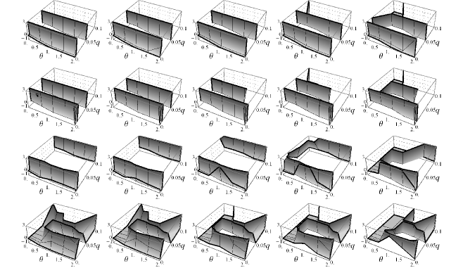
(a) 3D bias surfaces for $\hat{D}_{\mathrm{CL2}}$. The almost vertical surfaces indicate onset of severe positive bias.

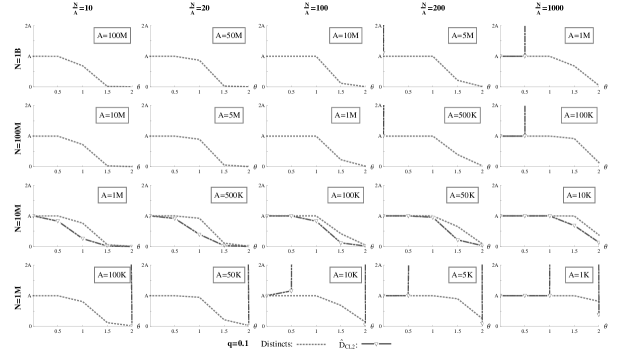
(b) $\hat{D}_{\mathrm{CL2}}$ at $q=0.1$. Even at this high sampling fraction, $\hat{D}_{\mathrm{CL2}}$ is accurate only at 10M population size. Surprisingly, it is inaccurate at the lower population size of 1M, as well as at higher sizes.

Figure 11: The highly irregular bias behavior of the Chao-Lee estimators. The difference between $\hat{D}_{\mathrm{CL1}}$ and $\hat{D}_{\mathrm{CL2}}$ is insignificant, hence only $\hat{D}_{\mathrm{CL2}}$ shown.

References

- [1] Morton M. Astrahan, Mario Schkolnick, and Kyu-Young Whang. Approximating the number of unique values of an attribute without sorting. Inf. Syst., 12(1):11–15, 1987.
- [2] Kevin Beyer, Rainer Gemulla, Peter J. Haas, Berthold Reinwald, and Yannis Sismanis. Distinct-value synopses for multiset operations. Commun. ACM, 52:87–95, October 2009.
- [3] J. Bunge and M. Fitzpatrick. Estimating the number of species: A review. Journal of the American Statistical Association, 88(421):pp. 364–373, 1993.
- [4] K. P. Burnham and W. S. Overton. Estimation of the size of a closed population when capture probabilities vary among animals. Biometrika, 65(3):pp. 625–633, 1978.
- [5] K. P. Burnham and W. S. Overton. Robust estimation of population size when capture probabilities vary among animals. Ecology, 60(5):pp. 927–936, 1979.
- [6] Anne Chao. Nonparametric estimation of the number of classes in a population. Scandinavian Journal of Statistics, 11(4):pp. 265–270, 1984.
- [7] Anne Chao and Shen-Ming Lee. Estimating the number of classes via sample coverage. Journal of the American Statistical Association, 87(417):pp. 210–217, 1992.
- [8] Anne Chao, M.-C. Ma, and Mark C. K. Yang. Stopping rules and estimation for recapture debugging with unequal failure rates. Biometrika, 80(1):pp. 193–201, 1993.
- [9] Moses Charikar, Surajit Chaudhuri, Rajeev Motwani, and Vivek R. Narasayya. Towards estimation error guarantees for distinct values. In PODS, pages 268–279, 2000.
- [10] Surajit Chaudhuri, Rajeev Motwani, and Vivek R. Narasayya. Random sampling for histogram construction: How much is enough? In SIGMOD Conference, pages 436–447, 1998.
- [11] J. N. Darroch and D. Ratcliff. A note on capture-recapture estimation. Biometrics, 36(1):pp. 149–153, 1980.
- [12] Warren W. Esty. Confidence intervals for the coverage of low coverage samples. The Annals of Statistics, 10(1):pp. 190–196, 1982.
- [13] Warren W. Esty. The efficiency of good’s nonparametric coverage estimator. The Annals of Statistics, 14(3):pp. 1257–1260, 1986.
- [14] Philippe Flajolet and G. Nigel Martin. Probabilistic counting algorithms for data base applications. J. Comput. System Sci., 31(2):182–209, 1985. Special issue: Twenty-fourth annual symposium on the foundations of computer science (Tucson, Ariz., 1983).
- [15] I. J. Good. The population frequencies of species and the estimation of population parameters. Biometrika, 40(3/4):pp. 237–264, 1953.
- [16] I. J. Good and G. H. Toulmin. The number of new species, and the increase in population coverage, when a sample is increased. Biometrika, 43(1/2):pp. 45–63, 1956.
- [17] Leo A. Goodman. On the estimation of the number of classes in a population. Ann. Math. Statistics, 20:572–579, 1949.
- [18] H. L. Gray and W. R. Schucany. The generalized jackknife statistic. Marcel Dekker Inc., New York, 1972. Statistics Textbooks and Monographs, Vol. 1.
- [19] Peter J. Haas, Jeffrey F. Naughton, S. Seshadri, and Lynne Stokes. Sampling-based estimation of the number of distinct values of an attribute. In VLDB, pages 311–322, 1995.
- [20] Peter J. Haas and Lynne Stokes. Estimating the number of classes in a finite population. Journal of the American Statistical Association, 93(444):pp. 1475–1487, 1998.
- [21] Wen-Chi Hou, Gultekin Özsoyoglu, and Baldeo K. Taneja. Statistical estimators for relational algebra expressions. In PODS, pages 276–287, 1988.
- [22] Michael Mitzenmacher. A brief history of generative models for power law and lognormal distributions. Internet Math., 1(2):226–251, 2004.
- [23] F. Mosteller. Questions and answers. American Statistician, 3:12–13, 1949.
- [24] Jeffrey F. Naughton and S. Seshadri. On estimating the size of projections. In ICDT, pages 499–513, 1990.
- [25] Gultekin Özsoyoglu, Kaizheng Du, A. Tjahjana, Wen-Chi Hou, and D. Y. Rowland. On estimating count, sum, and average. In DEXA, pages 406–412, 1991.
- [26] Herbert E. Robbins. Estimating the total probability of the unobserved outcomes of an experiment. The Annals of Mathematical Statistics, 39(1):pp. 256–257, 1968.
- [27] A. Schlosser. On estimation of the size of the dictionary of a long text on the basis of a sample. Engineering Cybernetics, 19:pp. 97–102, 1981.
- [28] H. S. Sichel. Anatomy of the generalized inverse gaussian-poisson distribution with special applications to bibliometric studies. Inf. Process. Manage., 28(1):5–18, 1992.
- [29] Eric P. Smith and Gerald van Belle. Nonparametric estimation of species richness. Biometrics, 40(1):pp. 119–129, 1984.
- [30] Tabular Analysis. Data warehouse market forecast 2017-2022.