Charmed mesons at finite temperature and chemical potential

Abstract

We compute the masses of the pseudoscalar mesons $\pi^{+}$, $K^{0}$ and $D^{+}$ at finite temperature and baryon chemical potential. The computations are based on a symmetry-preserving Dyson-Schwinger equation treatment of a vector-vector four quark contact interaction. The results found for the temperature dependence of the meson masses are in qualitative agreement with lattice QCD data and QCD sum rules calculations. The chemical potential dependence of the masses provide a novel prediction of the present computation.

1 Introduction

Heavy-light mesons, like the $D$ and $B$, are interesting QCD bound states: they play an important role in the threshold dynamics of many of the so-called X,Y,Z exotic hadrons Briceno:2015rlt and also serve as a laboratory for studying chiral properties of the light $u$ and $d$ quarks in a medium at finite temperature $T$ and baryon density $\mu$ in different contexts. Great progress has been achieved in recent years in the study of their properties with lattice QCD methods, both in vacuum and at finite temperature Skull . In the continuum, however, although in principle the complex of the Schwinger-Dyson (DS) and Bethe-Salpeter (BS) equations provides an adequate framework, tremendous challenges still remain in describing simultaneously light- and heavy-flavored mesons in vacuum within a single model interaction–truncation scheme MT ; Krass ; Rojas:2014aka . On the other hand, there is pressing need for different pieces of information on properties of such mesons both in vacuum and at finite $T$ and $\mu$ for guiding experimental proposals at existing and forthcoming facilities. Examples are charmed-hadron production via $\bar{p}p$ annihilation processes Haidenbauer:2009ad ; Haidenbauer:2014rva ; Haidenbauer:2015vra , $J/\Psi$-nuclear bound states Krein:2010vp ; Tsushima:2011kh , production in heavy-ion collisions of exotic molecules like the $\Delta\bar{D}^{*}$ Carames:2016qhr . Having this in mind, in the present contribution we extend to finite $T$ and $\mu$ a model that gives a good description of the spectrum and leptonic decay constants of pseudoscalar mesons in vacuum F.E.S . The model is based on a confining, symmetry-preserving treatment of a vector-vector four fermion contact interaction as a representation of the gluon’s two-point Schwinger function used in kernels of DS equations, originally tuned to study the pion GutierrezGuerrero:2010md .

A potential problem with contact-interaction models is their nonrenormalizability, in that it can introduce gross violations of global and local symmetries because of ambiguities related to momentum shifts in divergent integrals. Here we use a subtraction scheme Battistel:1998tj that allows us to separate symmetry-violating parts in Bethe-Salpeter amplitudes in a way independent of choices of momentum routing in divergent integrals. The scheme has been used in the past within the Nambu–Jona-Lasinio (NJL) model in vacuum Battistel:2008fd , at finite $T$ and $\mu$  Farias and, more recently Farias:2016let , it was used to explain the reason for the failure of the model to explain lattice results for the chiral transition temperature in the presence of a chiral imbalance in quark matter.

We extend the subtraction scheme of Ref. F.E.S to finite $T$ and $\mu$; the situation is more complicated than in the vacuum because Lorentz covariance is broken at finite $T$ and $\mu$ and special care must be exercised to separate purely divergent contributions from thermal effects, which are finite and do not need regularization. After setting up the scheme, we calculate the masses of the pseudoscalar mesons $\pi^{+}$, $K^{0}$ and $D^{+}$ at finite $T$ and $\mu$ and compare results with those obtained recently using QCD sum rules Suzuki:2015est and those obtained earlier with the NJL model Blaschke:2011yv ; Gottfried:1992bz .

2 Dyson-Schwinger and Bethe-Salpeter equations at finite $\bm{T}$ and $\bm{\mu}$

The Dyson-Schwinger equation (DSE) for the full quark propagator $S_{f}(k)$ of flavor $f$ is given by (in Euclidean space)

$$S^{-1}_{f}(k)=i\not{k}+m_{f}+\int\frac{d^{4}q}{(2\pi)^{4}}\,g^{2}D_{\mu\nu}(k-q)\,\frac{\lambda^{a}}{2}\gamma_{\mu}S_{f}(q)\frac{\lambda^{a}}{2}\Gamma^{f}_{\nu}(q,k)\leavevmode\nobreak\ ,$$ (1)

where $m_{f}$ is the current-quark mass, $D^{\mu\nu}$ the full gluon propagator, and $\Gamma^{f}_{\nu}$ the full quark-gluon vertex. The mass $m_{\rm PS}$ of a pseudoscalar (PS) meson with one light ($f=l$) quark and one heavy ($f=h$) quark is the eigenvalue $P^{2}=-m^{2}_{\rm PS}$ that solves the homogeneous Bethe-Salpeter equation (BSE)

$$\Gamma^{lh}_{\rm PS}(k;P)=\int\frac{d^{4}q}{(2\pi)^{4}}K(k,q;P)S_{l}(q_{+})\Gamma^{lh}_{\rm PS}(q;P)S_{h}(q_{-})\leavevmode\nobreak\ ,$$ (2)

with $K(k,q;P)$ being the fully amputated quark-antiquark scattering kernel, where $q_{\pm}=q\pm\eta_{\pm}P$ and $\eta_{+}+\eta_{-}=1$. At finite $T$ and $\mu$, the four dimensional momentum integrals in Eqs. (1) and (2) become

$$\int\frac{d^{4}q}{(2\pi)^{4}}\,F(q)\rightarrow\frac{1}{\beta}\sum^{\infty}_{m=-\infty}\int\frac{d^{3}q}{(2\pi)^{3}}\,F(\omega_{m},{\bf q})\leavevmode\nobreak\ ,$$ (3)

where $\omega_{m}=(2m+1)\,\pi/\beta$ are the fermionic Matsubara frequencies with $\beta=1/T$ and $m\in\mathds{Z}$. The contact-interaction limit of full QCD is obtained by making the following replacements in Eqs. (1) and (2)

$$g^{2}D_{\mu\nu}(p-q)\rightarrow G\,\delta_{\mu\nu},\hskip 19.91684pt\Gamma^{a}_{\mu}\rightarrow\frac{\lambda^{a}}{2}\gamma_{\mu},\hskip 19.91684ptK(k,q;P)=-G\,\left(\frac{\lambda^{a}}{2}\gamma^{\mu}\right)\otimes\left(\frac{\lambda^{a}}{2}\gamma_{\mu}\right)\leavevmode\nobreak\ ,$$ (4)

where $G$ is an effective coupling constant with dimensions of (length)². In this limit, Eq. (1) becomes

$$S^{-1}_{f}({{\bf q}},\omega_{m})=i{\bm{\gamma}}\cdot{\bf q}+i\gamma_{4}\,\omega_{m}+M_{f}\leavevmode\nobreak\ ,$$ (5)

with $M_{f}=M_{f}(T,\mu)$ given by (the gap equation)

$$M_{f}=m_{f}+\frac{16}{3}G\,\left\{I_{\rm quad}(M_{f})-\int\frac{d^{3}q}{(2\pi)^{3}}\frac{M_{f}}{2E_{f}({\bf q})}\left[f^{-}(E_{f}({\bf q}))+f^{+}(E_{f}({\bf q}))\right]\right\}\leavevmode\nobreak\ ,$$ (6)

where

$$I_{\rm quad}(M^{2})=\int\frac{d^{4}q}{(2\pi)^{4}}\,\frac{1}{q^{2}+M^{2}}\leavevmode\nobreak\ ,\hskip 14.22636ptf^{\pm}(E)=\frac{1}{1+e^{\,\beta E^{\pm}}}\leavevmode\nobreak\ ,$$ (7)

with $E^{\pm}_{f}({\bf q})=E_{f}({\bf q})\pm\mu$, and $E_{f}(q)=({\bf q}^{2}+M^{2}_{f})^{1/2}$. The Bethe-Salpeter amplitude (BSA) contains only pseudo-scalar and pseudo-vector components:

$$\Gamma^{lh}_{\rm PS}(P)=\gamma_{5}\left[iE^{lh}_{\rm PS}(P)+\frac{1}{2M_{lh}}\gamma\cdotp P\,F^{lh}_{\rm PS}(P)\right]\leavevmode\nobreak\ ,$$ (8)

with $P=(\nu_{n},{\bf P})$, $\nu_{n}=2n\pi/\beta$, and the factor $M_{lh}=M_{l}M_{h}/(M_{l}+M_{h})$, where $M_{l}$ and $M_{h}$ are solutions of Eq. (6), is introduced for convenience. Using this in Eq. (2), the BSE of can be written F.E.S as a matrix equation involving the amplitudes $E^{lh}_{\rm PS}$ and $F^{lh}_{\rm PS}$. For comparison with earlier results in the literature that use the Random Phase Approximation (RPA), one needs to use only the pseudoscalar component $E^{lh}_{\rm PS}$ in $\Gamma^{lh}_{\rm PS}(P)$. The meson mass is obtained taking $\omega=m_{\rm PS}$ in the expression

$$0=1-\frac{G}{3}\,\Pi_{\rm PS}(\nu_{n}=-i\omega,{\bf P}=0)\leavevmode\nobreak\ ,$$ (9)

with

$$\Pi^{lh}_{\rm PS}(\nu_{n},{\bf P})=-\frac{1}{\beta}\sum^{\infty}_{m=-\infty}\int\frac{d^{3}q}{(2\pi)^{3}}{\rm{Tr}}\left[\gamma_{5}\gamma_{\mu}S_{l}({\bf q}_{+},\omega_{+})\gamma_{5}\,S_{h}({\bf q}_{-},\omega_{-})\gamma_{\mu}\right]\leavevmode\nobreak\ ,$$ (10)

where ${\bf q}_{\pm}={\bf q}\pm\eta_{\pm}\,{\bf P}$ and $\omega_{\pm}=\omega_{m}\pm\chi_{\pm}\,\nu_{n}$, where $\chi_{\pm}\in\mathds{Z}$. After taking a Dirac trace we can rewrite Eq. (10) as a sum of two terms: one that contains ultraviolet divergences

$$\Pi^{lh}_{\rm PS}(P)|_{\rm div}=8\int\frac{d^{4}q}{(2\pi)^{4}}\Bigg{\{}\frac{1}{q^{2}_{+}+M^{2}_{l}}+\frac{1}{q^{2}_{-}+M^{2}_{h}}-\left[P^{2}+\left(M_{h}-M_{l}\right)^{2}\right]\frac{1}{(q^{2}_{+}+M^{2}_{l})(q^{2}_{+}+M^{2}_{h})}\Bigg{\}}\leavevmode\nobreak\ ,$$ (11)

and another that is finite, given in terms of the Fermi-Dirac distributions $f^{\pm}(E)$ defined in Eq. (7):

$$\Pi^{lh}_{\rm PS}(P)|_{\rm fin} = -4\int\frac{d^{3}q}{(2\pi)^{3}}\Bigg{\{}\frac{f^{+}(E_{l}({\bf q}_{+}))+f^{-}(E_{l}({\bf q}_{+}))}{E_{l}({\bf q}_{+}))}+\frac{f^{+}(E_{h}({\bf q}_{-}))+f^{-}(E_{h}({\bf q}_{-}))}{E_{h}({\bf q}_{-})}$$ (12)

$$+ \frac{P^{2}+(M_{l}-M_{h})^{2}}{2E_{l}({\bf q}_{+})E_{h}({\bf q}_{-})}\Bigg{[}\frac{2E_{h}({\bf q}_{-})f^{-}(E_{l}({\bf q}_{+}))}{[\omega-E_{l}({\bf q}_{+})]^{2}-E^{2}_{h}({\bf q}_{-})}+\frac{2E_{l}({\bf q}_{+})f^{-}(E_{h}({\bf q}_{-}))}{[\omega+E_{h}({\bf q}_{-})]^{2}-E^{2}_{l}({\bf q}_{+})}$$

$$+ \frac{2E_{h}({\bf q}_{-})f^{+}(E_{l}({\bf q}_{+}))}{[\omega+E_{l}({\bf q}_{+})]^{2}-E^{2}_{h}({\bf q}_{-})}+\frac{2E_{l}({\bf q}_{+})f^{+}(E_{h}({\bf q}_{-}))}{[\omega-E_{h}({\bf q}_{-})]^{2}-E^{2}_{l}({\bf q}_{+})}\Bigg{]}\Bigg{\}}\leavevmode\nobreak\ .$$

In Eqs. (11) and (12), $P=(-i\omega,{\bf P})$. The problem with symmetry violations alluded to in the Introduction comes from the divergent part: it depends on the choice made for the partition of the momenta in the loop integral when using a cutoff regularization, i.e. it is not independent of $\eta_{\pm}$. Our scheme F.E.S to obtain symmetry-preserving expressions is to perform subtractions in divergent integrals:

$$\frac{1}{q^{2}_{\pm}+M^{2}_{l,h}} = \frac{1}{q^{2}+M^{2}}+\left(\frac{1}{q^{2}_{\pm}+M^{2}_{l,h}}-\frac{1}{q^{2}+M^{2}}\right)=\frac{1}{q^{2}+M^{2}}-\frac{(q^{2}_{\pm}-q^{2}+M^{2}_{l,h}-M^{2})}{\left(q^{2}+M^{2}\right)(q^{2}_{\pm}+M^{2}_{l,h})},$$ (13)

with $M$ being an arbitrary subtraction mass scale. One performs as many subtractions as necessary to obtain one finite integral. The final result is F.E.S

$$\Pi^{lh}_{\rm PS}(P)|_{\rm div} = \frac{3}{G}-\frac{3}{2G}\left(\frac{m_{l}}{M_{l}}+\frac{m_{h}}{M_{h}}\right)-8\left[P^{2}+(M_{l}-M_{h})^{2}\right]\left[I_{\rm log}(M)-Z_{0}(M^{2}_{l},M^{2}_{h},P^{2},M^{2})\right]$$ (14)

$$\,+8\,(\eta^{2}_{+}+\eta^{2}_{-})\,A_{\mu\nu}(M^{2})\,P_{\mu}P_{\nu}\leavevmode\nobreak\ ,$$

where $I_{\rm log}(M^{2})$ is a divergent integral and $Z_{0}(M^{2}_{l},M^{2}_{h},P^{2},M^{2})$ is a finite integral

$$I_{\rm log}(M^{2})=\int\frac{d^{4}q}{(2\pi)^{4}}\,\frac{1}{\left(q^{2}+M^{2}\right)^{2}}\leavevmode\nobreak\ ,\hskip 14.22636ptZ_{0}(M^{2}_{l},M^{2}_{h},P^{2},M^{2})=\frac{1}{(4\pi)^{2}}\int^{1}_{0}dz\ln\left[\frac{H(z,P^{2})}{M^{2}}\right]\leavevmode\nobreak\ ,$$ (15)

with $H=z(z-1)P^{2}-z(M^{2}_{l}-M^{2}_{h})+M^{2}_{l}$, and $A_{\mu\nu}(M^{2})$ is another divergent integral

$$A_{\mu\nu}(M^{2})=\int\frac{d^{4}q}{(2\pi)^{4}}\frac{4q_{\mu}q_{\nu}-(q^{2}+M^{2})\delta_{\mu\nu}}{(q^{2}+M^{2})^{3}}\leavevmode\nobreak\ .$$ (16)

The finite integral in Eq. (15) is obtained by integrating over momentum, removing any regularization implicitly assumed. Clearly, the term proportional to $A_{\mu\nu}(M^{2})$ is not independent of $\eta_{\pm}$ and, therefore, violates translation symmetry. Similar expressions appear also in Ward-Takahashi identities F.E.S . Since there are regularizations schemes, like dimensional regularization, where $A_{\mu\nu}(M^{2})=0$ automatically, it is a natural prescription for obtaining symmetry-preserving amplitudes to demand the vanishing of $A_{\mu\nu}(M^{2})$ (and of all other similar terms that appear in other amplitudes, see e.g. Ref. F.E.S ), independently of the regularization used to regulate $I_{\rm quad}(M^{2})$ and $I_{\rm log}(M^{2})$.

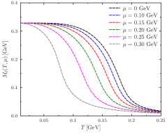
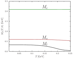
Figure 1: Constituent quark mass as function of $T$ for different values of $\mu$.

The mass scale $M$ in Eq. (13) is arbitrary; it appears in the divergent integrals $I_{\rm log}(M^{2})$ and $I_{\rm quad}(M^{2})$ and in the finite integral $Z_{0}(M^{2}_{l},M^{2}_{h},P^{2},M^{2})$. Since the model is nonrenormalizable, the integrals $I_{\rm log}(M^{2})$ and $I_{\rm quad}(M^{2})$ cannot be removed, of course. One can use an explicit regulator to evaluate the integrals and fit the regulator to physical quantities, like the quark condensate or hadron masses, or one could also fit the integrals directly to physical quantities. In either case, the fit to physical quantities is $M$-dependent, that is, physical quantities would “run with $M$”, very much like in renormalizable quantum field theories where all masses and other quantities are running functions of a mass scale that enters the theory via the regularization scheme. Here we present results using an explicit three-dimensional cutoff $\Lambda$ to regulate the divergent integrals $I_{\rm log}(M^{2})$ and $I_{\rm quad}(M^{2})$, and take $M=M_{h}$, for simplicity—further discussions on this will be presented elsewhere.

3 Numerical results and conclusions

The free parameters are: $G$, $\Lambda$ and $m_{f}$. Taking $\Lambda=0.653\leavevmode\nobreak\ {\rm GeV}$, $G\Lambda^{2}=19.26$, $m_{l}=m_{u}=m_{d}=0.005$ GeV, $m_{s}=0.161$ GeV and $m_{c}=1.544$ GeV, one obtains for the meson masses in vacuum: $m_{\pi}=0.139$ GeV, $m_{K^{0}}=0.493$ GeV and $m_{D^{+}}=1.864$ GeV. It is worth mentioning that we obtain for the constituent quark masses in vacuum the following values: $M_{l}=0.328$ GeV, $M_{s}=0.599$ GeV and $M_{c}=2.095$ GeV. The results for the $T$ dependence of $M_{l}$ for different values of $\mu$, obtained from the DSE in Eq. (6), are shown in the left panel of Fig. 1. Clearly, as $\mu$ increases, the (pseudo) critical temperature for chiral restoration decreases as $\mu$ increases, as expected. On the right panel of the figure, the temperature dependence of $M_{l}$, $M_{s}$ and $M_{c}$ for zero chemical potential: also as expected, as the current quark mass increases, the effect of the temperature becomes less important, even close to and above the pseudocritical temperature.

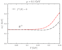
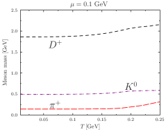
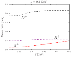
Figure 2: Meson masses as functions of $T$ for two typical values of $\mu$. Top panels: $m_{\pi^{+}}$ calculated with and without the Fermi-Dirac distributions $f^{\pm}(E)$ in the BSE. Bottom panels: masses calculated without the $f^{\pm}(E)$ in the BSE.

The last point raises the question on the importance of the Fermi-Dirac distribution functions, $f^{\pm}(E)$, in the BSE for the masses of the mesons—physically, they represent the contributions of thermally activated quark-antiquark pairs in the bound state. The answer to this question is shown in the top panels of Fig. 2: for sufficiently low values of $\mu$, the $f^{\pm}(E)$ play no significant role for $T$ smaller than the pseudocritical temperature and can, to a good approximation, be neglected. This is an important feature, as it simplifies considerably the calculations of thermal effects on hadron masses, as all $T$ and $\mu$ effects below the crossover are captured by the $T$ and $\mu$ dependence of the constituent quark masses. In the bottom panel of Fig. 2, we show the results for the mesons masses neglecting the Fermi-Dirac distributions: the results are in good quantitative agreement with early calculations using the NJL model Blaschke:2011yv ; Gottfried:1992bz . It also agrees with a very recent calculation using a chiral constituent quark model, using as input $T$ and $\mu$ dependent quark masses and quark-meson couplings Carames:2016qhr , Finally, our results are also in qualitative agreement with a recent calculation using QCD sum rules Suzuki:2015est —this last reference points to earlier calculations, that obtained the opposite trend or the $D$ meson mass. We also mention that recent lattice results Skull show that the masses of $D$ mesons increase, and become broader.

As perspectives, concrete calculations of production rates of exotic hadronic molecules in heavy-ion collisions Briceno:2015rlt ; Carames:2016qhr and of transport properties of charmed hadrons Ghosh:2015mda are top priority. In addition, it would be important to contrast results using confining chiral models. Of particular interest to us are those models inspired in QCD formulated in Coulomb gauge Bicudo:1991kz ; Fontoura:2012mz , and those based on chiral soliton models Krein:1988sb ; Krein:1988vh .

We thank B. El-Bennich for valuable discussions. Work partially by Conselho Nacional de Desenvolvimento Científico e Tecnológico - CNPq, Grants No. 305894/2009-9 (G.K.) and 140041/2014-1 (F.E.S.) and Fundação de Amparo à Pesquisa do Estado de São Paulo-FAPESP, Grant No. 2013/01907-0 (G.K.).

References

- (1) R. A. Briceno et al., Chin. Phys. C 40, 042001 (2016).
- (2) See J.-I. Skullerud and A. Kelly, these proceedings.
- (3) P. Maris and P. C. Tandy, Nucl. Phys. B, Proc. Suppl. 161, 136 (2006).
- (4) M. Gómez-Rocha, T. Hilger and A. Krassnigg, Few Body Syst. 56, 475 (2015).
- (5) E. Rojas, B. El-Bennich and J. P. B. C. de Melo, Phys. Rev. D 90, 074025 (2014).
- (6) J. Haidenbauer and G. Krein, Phys. Lett. B 687, 314 (2010).
- (7) J. Haidenbauer and G. Krein, Phys. Rev. D 89, 114003 (2014).
- (8) J. Haidenbauer and G. Krein, Phys. Rev. D 91, 114022 (2015).
- (9) G. Krein, A. W. Thomas and K. Tsushima, Phys. Lett. B 697, 136 (2011).
- (10) K. Tsushima et al. , Phys. Rev. C 83, 065208 (2011).
- (11) T. F. Caramés et al. , Phys. Rev. D 94, 034009 (2016).
- (12) F. E. Serna, M.A. Brito, and G. Krein, AIP Conf. Proc. 1701, 100018 (2016).
- (13) L. X. Gutierrez-Guerrero et al. Phys. Rev. C 81, 065202 (2010).
- (14) O. A. Battistel and M. C. Nemes, Phys. Rev. D 59, 055010 (1999).
- (15) O. A. Battistel, G. Dallabona and G. Krein, Phys. Rev. D 77 (2008) 065025.
- (16) R. L. S. Farias et al., Phys. Rev. C 77, 065201 (2008); Phys. Rev. C 73, 018201 (2006); Nucl. Phys. A 790, 332 (2007).
- (17) R. L. S. Farias, D. C. Duarte, G. Krein and R. O. Ramos, Phys. Rev. D 94, 074011 (2016).
- (18) K. Suzuki, P. Gubler and M. Oka, Phys. Rev. C 93, 045209 (2016).
- (19) D. Blaschke, P. Costa and Y. L. Kalinovsky, Phys. Rev. D 85, 034005 (2012).
- (20) F. O. Gottfried and S. P. Klevansky, Phys. Lett. B 286, 221 (1992).
- (21) S. Ghosh et al. Phys. Rev. C 93, 045205 (2016)
- (22) P. J. A. Bicudo et al., Phys. Rev. D 45, 1673 (1992).
- (23) C. E. Fontoura, G. Krein and V. E. Vizcarra, Phys. Rev. C 87, 025206 (2013).
- (24) G. Krein, P. Tang and A. G. Williams, Phys. Lett. B 215, 145 (1988).
- (25) G. Krein, P. Tang, L. Wilets and A. G. Williams, Phys. Lett. B 212, 362 (1988).