Standing on the shoulders of Dwarfs: the Kepler asteroseismic LEGACY sample I — oscillation mode parameters
Abstract
The advent of space-based missions like Kepler has revolutionized the study of solar-type stars, particularly through the measurement and modeling of their resonant modes of oscillation. Here we analyze a sample of 66 Kepler main-sequence stars showing solar-like oscillations as part of the Kepler seismic LEGACY project. We use Kepler short-cadence data, of which each star has at least 12 months, to create frequency power spectra optimized for asteroseismology. For each star we identify its modes of oscillation and extract parameters such as frequency, amplitude, and line width using a Bayesian Markov chain Monte Carlo ‘peak-bagging’ approach. We report the extracted mode parameters for all 66 stars, as well as derived quantities such as frequency difference ratios, the large and small separations and ; the behavior of line widths with frequency and line widths at with , for which we derive parametrizations; and behavior of mode visibilities. These average properties can be applied in future peak-bagging exercises to better constrain the parameters of the stellar oscillation spectra. The frequencies and frequency ratios can tightly constrain the fundamental parameters of these solar-type stars, and mode line widths and amplitudes can test models of mode damping and excitation.
Subject headings:
Asteroseismology – stars: evolution – stars: oscillations – stars: fundamental parameters1. Introduction
The study of stars and extrasolar planets via the properties of their host stars has experienced a revolution in recent years (Chaplin & Miglio 2013; Christensen-Dalsgaard 2016). This largely arose from the successful application of asteroseismology using observations from the CoRoT (Baglin et al. 2009) and Kepler missions (Gilliland et al. 2010). This application has been made possible by extracting high-precision parameters from the stellar frequency-power spectra owing to the long time-baseline and photometric quality of these space missions.
Asteroseismology allows the determination of fundamental stellar parameters such as mass, radius, and age through modeling of individual mode frequencies or frequency-difference ratios. The Kepler mission has already provided stellar parameters for a number of stars, including planetary hosts, using average seismic parameters (Chaplin et al. 2011a, 2014; Silva Aguirre et al. 2012; Huber et al. 2013), individual frequencies (Christensen-Dalsgaard et al. 2010; Basu et al. 2010; Howell et al. 2012; Metcalfe et al. 2012, 2014, 2015; Van Eylen et al. 2014; Lund et al. 2014c; Campante et al. 2015; Silva Aguirre et al. 2015), and frequency-difference ratios (Silva Aguirre et al. 2013, 2015; Lebreton & Goupil 2014).
The high precision of extracted mode frequencies further allows the study of ionization zones and the convective envelope boundary from acoustic glitches (Houdek & Gough 2007; Silva Aguirre et al. 2011; Mazumdar et al. 2014; Verma et al. 2014), and one may also learn about the physics of the excitation and damping of the oscillation modes from measured mode line widths, amplitudes, and visibilities (Houdek et al. 1999; Houdek 2006; Samadi et al. 2005, 2007; Belkacem et al. 2012).
Frequencies and line widths have been reported for several solar-like and subgiant stars observed by Kepler by Appourchaux et al. (2012b, a, 2014a), and planet-hosting stars by Davies et al. (2016). In this paper we analyze a sample of 66 main-sequence (MS) solar-like stars observed for at least 12 months by the Kepler mission. We extracted mode parameters by ‘peak-bagging’111First coined by Roger Ulrich circa 1983 (private communication) from the analogy to hill climbing where it refers to reaching the summits of a collection of peaks, the term was later re-introduced by Appourchaux (2003b). the frequency-power spectra of the stars using a Markov chain Monte Carlo (MCMC) method (Handberg & Campante 2011) and used the Bayesian quality control presented by Davies et al. (2016). For each star we report values for the mode frequencies, amplitudes, line widths, and visibilities. Additionally, we provide summary descriptions for each of the above quantities, such as average seismic parameters derived from the frequencies and prescriptions of the mode line widths against frequency. The frequencies reported here will be modeled in the accompanying paper by Silva Aguirre et al. (2016, hereafter Paper II). The lessons learned from the presented analysis will be useful for the study of MS solar-like oscillators with the TESS (Ricker et al. 2014) and PLATO (Rauer et al. 2013) missions, and the continued analysis of these data from K2 (Chaplin et al. 2015; Lund et al. 2016a, b).
The paper is structured as follows: Section 2 describes the target sample, including the preparation of Kepler data and spectroscopic properties. Section 3 is devoted to the parameter estimation from the MCMC peak-bagging, including a description of the fitting strategy, the adopted Bayesian quality assurance, and the derivation of frequency difference ratios and their correlations. In Section 4 we present our results from the peak-bagging for the mode frequencies, focusing specifically on frequency errors and average seismic parameters in Section 4.1; amplitudes in Section 4.2; line widths in Section 4.3; and visibilities in Section 4.4. In Section 5 we give an example of the output generated for each of the analyzed stars. We conclude in Section 6.
2. Target sample
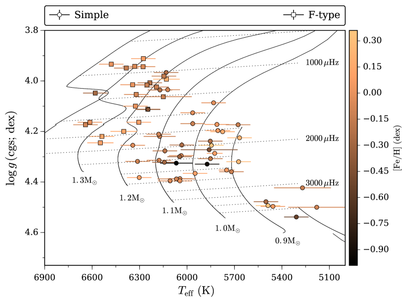
Our sample consists of 66 solar-type oscillators observed by the Kepler satellite, all part of the KASC (Kjeldsen et al. 2010) working group 1 (WG1) sample of solar-like p-mode oscillators. All stars have short-cadence (SC; ) observations with an observing base line of at least 12 months, and represent some of the highest signal-to-noise solar-like oscillators observed by Kepler. The sample consists only of main-sequence (MS) and slightly more evolved subgiant stars. These have frequency structures corresponding to the ‘Simple’ or ‘F-type’ categories by Appourchaux et al. (2012a), i.e., none of the stars show obvious bumped dipole modes. The sample was peak-bagged as part of the Kepler dwarf seismic ‘LEGACY’ project, with the asteroseismic modeling of extracted parameters presented in Paper II. In Figure 1 the sample is shown in a Kiel-diagram ( vs. ), with parameters adopted from Paper II; for additional details on the sample see Table 1. We note that all targets from the Appourchaux et al. (2014b) study of oscillation mode line widths (which included data up to Quarter 12) are part of our sample, with the exception of KIC 3424541, 3733735, 10355856, and 10909629. These four stars were classified as F-type by Appourchaux et al. (2014b), but were omitted from our sample because of possible mixed-mode structures.
| KIC | Popular | Kp | Number of | Category | Braketing | Missing | [Fe/H] | LOS | |||||
|---|---|---|---|---|---|---|---|---|---|---|---|---|---|
| name | (mag) | () | () | modes | Quarters | Quarters | (K) | (dex) | (cgs; dex) | () | () | ||
| F-like | |||||||||||||
| F-like | |||||||||||||
| Simple | |||||||||||||
| F-like | |||||||||||||
| Cassie | F-like | ||||||||||||
| Java | Simple | ||||||||||||
| Simple | |||||||||||||
| Vitto | Simple | ||||||||||||
| Kitty | Simple | ||||||||||||
| F-like | 5 | 5 | |||||||||||
| Simple | |||||||||||||
| Perky | Simple | ||||||||||||
| Nunny | Simple | ||||||||||||
| Saxo2 | Simple | ||||||||||||
| Baloo | F-like | ||||||||||||
| Saxo | Simple | ||||||||||||
| F-like | |||||||||||||
| Fred | Simple | ||||||||||||
| F-like | |||||||||||||
| Simple | 3 | 3 | |||||||||||
| Bagheera | F-like | ||||||||||||
| Simple | |||||||||||||
| Simple | |||||||||||||
| Simba | Simple | ||||||||||||
| F-like | |||||||||||||
| Simple | |||||||||||||
| Akela | F-like | ||||||||||||
| Simple | |||||||||||||
| Doris | Simple | ||||||||||||
| Simple | 3 | 3 | |||||||||||
| Simple | |||||||||||||
| Horace | Simple | ||||||||||||
| Arthur | Simple | 1 | 1 | ||||||||||
| Simple | |||||||||||||
| Simple | |||||||||||||
| Simple | |||||||||||||
| Pucky | Simple | ||||||||||||
| Java2 | Simple | ||||||||||||
| Simple | 2 | 2 | |||||||||||
| Simple | |||||||||||||
| Carlsberg | Simple | ||||||||||||
| Punto | F-like | 5 | 5 | ||||||||||
| F-like | |||||||||||||
| F-like | |||||||||||||
| Simple | |||||||||||||
| F-like | 6 | 6 | |||||||||||
| F-like | |||||||||||||
| Simple | |||||||||||||
| Simple | 2 | 2 | |||||||||||
| Simple | |||||||||||||
| Simple | |||||||||||||
| F-like | |||||||||||||
| Pinocha | Simple | ||||||||||||
| Manon | Simple | ||||||||||||
| Mowgli | Simple | ||||||||||||
| F-like | 2 | 2 | |||||||||||
| Rudy | Simple | ||||||||||||
| F-like | |||||||||||||
| Tinky | F-like | ||||||||||||
| Simple | 2 | 2 | |||||||||||
| Dushera | Simple | ||||||||||||
| F-like | |||||||||||||
| 16 Cyg A | Simple | 4 | 4 | ||||||||||
| 16 Cyg B | Simple | 4 | 4 | ||||||||||
| Barney | Simple | ||||||||||||
| F-like |
- •
2.1. Data preparation
For most targets, data were taken continuously from Quarter 5 (Q5) through Q17. To minimize gaps in the time series, data from the initial short quarters (Q0 or Q1) were omitted unless continuous with the subsequent data. Table 1 lists the quarters used for each target. Light curves were constructed from pixel data downloaded from the KASOC database222www.kasoc.phys.au.dk, using the procedure developed by S. Bloemen (private comm.) to define pixel masks for aperture photometry. The light curves were then corrected using the KASOC filter (see Handberg & Lund 2014). Briefly, the light curves were first corrected for jumps and concatenated. They were then median filtered using two filters of different widths — one long, one short — with the final filter being a weighted sum of the two filters based on the variability in the light curve. For the four Kepler objects of interest (KOIs) in the sample (KICs 3632418, 9414417, 9955598, and 10963065) an iterative removal of the planetary transits was performed based on the planetary phase-curve (see Handberg & Lund 2014 for further details).
The power density spectrum (PDS) returned from the KASOC filter is made from a weighted least-squares sine-wave fitting, single-sided calibrated, normalized to Parseval’s theorem, and converted to power density by dividing by the integral of the spectral window (Kjeldsen & Frandsen 1992; Kjeldsen 1992).
2.2. Atmospheric and stellar parameters
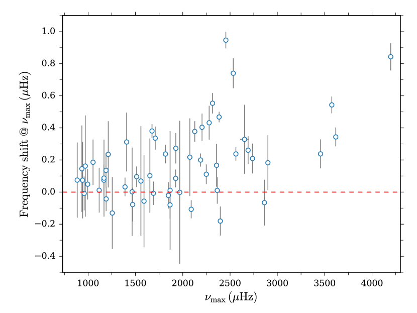
We have obtained atmospheric parameters from the Stellar Parameters Classification tool (SPC; see Buchhave et al. 2012), with data from the Tillinghast Reflector Echelle Spectrograph (TRES; Szentgyorgyi & Furész 2007; Fürész 2008) on the 1.5-m Tillinghast telescope at the F. L. Whipple Observatory. Information from the SPC analysis is available on the Kepler Community Follow-up Observing Program (CFOP) website333https://cfop.ipac.caltech.edu/home/. In the SPC derivation of parameters, values were fixed to the asteroseismic values given in Chaplin et al. (2014) to decrease the impact on uncertainties from correlations between , , and . We added in quadrature to the derived uncertainties on and systematic uncertainties of and , as suggested by Torres et al. (2012). For a subset of targets, spectroscopic values were taken from the literature (Table 1). We also list in Table 1 the line-of-sight (LOS) velocities derived from the SPC analysis, which should be used in any modeling efforts using individual frequencies to account for the Doppler shift of the frequencies (Davies et al. 2014b). In Figure 2 we show the values of these Doppler frequency shifts, which in some cases exceed the uncertainties on the individual frequencies. Even if the frequency shift is small compared to the uncertainties on the mode frequencies, it is systematic and should therefore always be corrected to avoid biases in the stellar modeling. The SPC LOS values have been corrected by to put the velocities onto the IAU system. This correction is primarily accounting for the fact that the CfA library of synthetic spectra does not include the solar gravitational redshift. Stellar parameters used in this paper, such as masses and radii, are adopted from the modeling effort presented in Paper II.
2.3. Sun-as-a-star data
As part of the project, the Sun was fitted in the same manner as the sample targets (see Section 3). This was done primarily to test the modeling efforts presented in Paper II against a known reference, and at the same time to assess the returns from the peak-bagging. The power spectrum was produced from data from VIRGO444Variability of Solar Irradiance and Gravity Oscillations (Fröhlich 2009) on-board the SoHO555Solar and Heliospheric Observatory spacecraft (Fröhlich et al. 1995; Frohlich et al. 1997). Specifically, a time series was created from a weighted sum of the green and red channels of the VIRGO Sun photometers (SPM) with central wavelengths of 500 nm (green), and 862 nm (red). Weights were selected such that the response-function weighted centroid wavelength from the two SPM channels matched that from the Kepler response function (641.7 nm). The two-component light curves were filtered individually using a 30-day median filter and then summed in relative flux units with the appropriate weights (green: 0.785; red: 0.215). The solar time series had a length of 1150 days (corresponding to years, or the approximate duration of 13 Quarters). This is the typical time series length for targets in the sample. To find the level to which the spectrum should be degraded, the magnitude distribution was computed for the sample, including also stars that have a mixed-mode character. The median magnitude of closely matches that of KIC 9139151 and so noise was added to the solar time series to match the level of this star.
The solar data set will primarily be used for estimates relating to frequencies, such as and , but not for analysis of line widths, amplitudes, or visibilities. This is because one cannot, with the simple weighting of relatively narrow band filters done here, assume that the measurements of amplitudes and visibilities adhere strictly to what would be observed with Kepler.
3. Parameter estimation
3.1. Oscillation spectrum model
To model the power spectrum, we described each oscillation mode as a Lorentzian function (), which corresponds to the shape of a stochastically-excited and intrinsically-damped mode (Batchelor 1953; Kumar et al. 1988):
| (3.1) |
Each mode is characterized by the frequency of the zonal () component, a height , a FWHM mode width , and a rotational splitting (assumed constant with frequency; see Lund et al. 2014b, for a discussion of the impact of differential rotation on the constancy of ). In , is the geometrical factor that sets the relative visibilities between the (azimuthal) -components as a function of the stellar inclination (see, Dziembowski 1977; Gizon & Solanki 2003); denotes the squared visibility (power units) of a non-radial mode relative to a radial mode at the same frequency, i.e.,
| (3.2) |
from the spatial filtering resulting from integrating the intensity for a mode of a given degree over the stellar surface; then denotes the height of the radial mode of order . The use of assumes equipartition of energy between modes of different angular degrees, thus only with a dependence on frequency. This is a good assumption for stochastically excited low degree high order acoustic modes, observed for many lifetimes (see, e.g., Christensen-Dalsgaard & Gough 1982).
The full model to fit to the power spectrum is then given by a series of the Lorentzian functions in Equation 3.1 as
| (3.3) |
Here denotes the adopted background function; is a constant white shot-noise component; describes the apodization of the signal power at frequency from the -minute sampling of the temporal signal (see, e.g., Chaplin et al. 2011c; Kallinger et al. 2014), and is given by:
| (3.4) |
where gives the integration time for the observations666In Kepler equals the sampling time wherefore sometimes is given as , where is the Nyquist frequency — this is, however, an imprecise definition, because relates to the sampling time whereas the apodization relates to the integration time.. For the background we used the function (Harvey et al. 1993; Andersen et al. 1994):
| (3.5) |
which characterizes a temporal signal from granulation having an exponentially decaying autocovariance, with a power of the temporal decay rate as ; gives the characteristic time scale of the th background component; the corresponding root-mean-square (rms) variation of the component in the time domain. The normalization constants are such that the integral (for positive frequencies) of the background component equals , in accordance with the Parseval-Plancherel theorem (see, e.g., Michel et al. 2009; Karoff et al. 2013; Kallinger et al. 2014).
In fitting Equation 3.3 to the power spectrum, we varied the mode amplitude (square-root of integrated mode power) rather than the mode height to decrease the correlation with (Toutain & Appourchaux 1994). To obtain the height () in power density units from the varied amplitude () we used the relation (Fletcher et al. 2006; Chaplin et al. 2008b):
| (3.6) |
This is a valid approximation for a single-sided power spectrum when the modes are well resolved, i.e., when the observing duration greatly exceeds the mode life time . We note that and were varied for radial modes only (), and then linearly interpolated to the frequencies of the non-radial modes. The fitting of the power spectrum then finally involved estimating the parameters .
3.2. Fitting strategy
Parameters were estimated in a Bayesian manner from a global peak-bagging fit to the power spectrum including all parameters (see, e.g., Handberg & Campante 2011). This was done by mapping the posterior probability of the parameters given the data and any prior information , which from Bayes’ theorem is given as:
| (3.7) |
Here is the prior probability assigned to the parameters given , and is the likelihood of the observed data given the parameters . , known as the evidence, is given by the integral of the numerator over the full parameter space, and thus acts as a normalization. The evidence is unnecessary in the mapping of the relative posterior distribution, so we end up mapping:
| (3.8) |
where logarithmic units are adopted for numerical stability, and is a constant. Assuming a 2-d.o.f. statistic for the power spectrum relative to the limit spectrum in Equation 3.3 (Gabriel 1994), the logarithm of the likelihood for a given observed power, , relates to the limit spectrum, , as (see Duvall & Harvey 1986; Anderson et al. 1990; Toutain & Appourchaux 1994):
| (3.9) |
Mapping of Equation 3.7 was performed using an affine invariant ensemble Markov chain Monte Carlo (MCMC) sampler (see Goodman & Weare 2010), specifically via the Python implementation emcee by Foreman-Mackey et al. (2013). For a given fit we employed 500 so-called walkers that were initiated by sampling from the priors of the model parameters (see Section 3.2.2). Each of these was run for at least 2000 steps. We further adopted parallel tempering using five temperatures, with tempering parameters determined according to Benomar et al. (2009), and a thinning of the MCMC chains by a factor of 10. As part of the post-processing, the appropriate burn-in for a given target and whether sufficient mixing had been achieved was determined by (1) visual inspection of the chain traces, (2) using the Geweke diagnostic (Geweke 1992), and (3) by assessing the length of the chain compared to the autocorrelation time (giving the number of independent draws from the target distribution).
Final parameter estimates were obtained from the median (frequencies) or mode (amplitudes, line widths, and visibilities) of the marginalized posterior probability density functions (PDFs) — with the MCMC sampling the marginalization is obtained naturally and the PDF for a given parameter is simply given by the normalized distribution of the samples of the parameter. A measure for the parameter uncertainty is given by the credible interval as the interval spanning the highest probability density (HPD) of the PDF.
3.2.1 Mode identification and initial guesses
Before the peak-bagging can commence, initial guesses must be defined for the mode-frequencies to include in Equation 3.3, and the modes must further be identified in terms of their angular degree . For acoustic modes of high radial order and low angular degree the frequencies may be approximated by the asymptotic relation (Tassoul 1980; Scherrer et al. 1983):
| (3.10) |
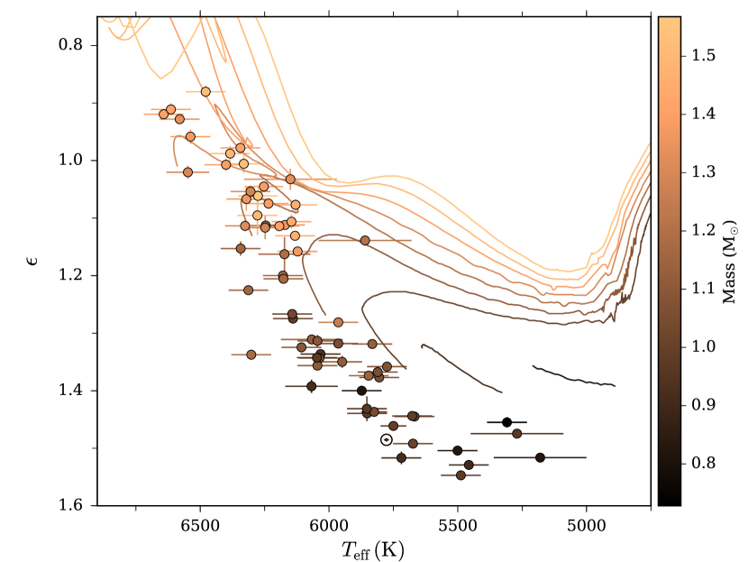
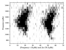
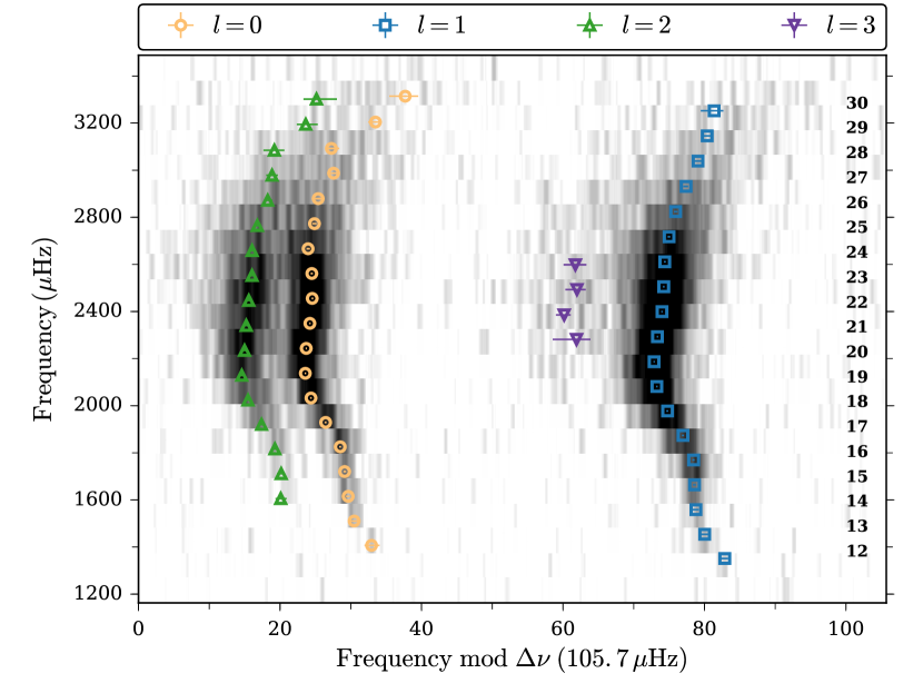
Here is the large separation, given by the average frequency spacing between consecutive overtones for modes of a given ; is a dimensionless offset sensitive to the surface layers (see, e.g., Gough 1986; Pérez Hernández & Christensen-Dalsgaard 1998; Roxburgh 2016); is sensitive to the sound-speed gradient near the stellar core (Scherrer et al. 1983; Christensen-Dalsgaard 1993). Mode identification was then, by and large, achieved via visual inspection of échelle diagrams (Grec et al. 1983; Bedding 2011). Here, modes of a given will form vertical ridges for the correct average large separation. The identification of and radial order was checked against the relation for as a function of (Figure 3), where can be found from the échelle diagram (Figure 4) by the vertical position of the radial degree () ridge (see White et al. 2011b, a).
For this study, consisting of high S/N oscillation signals, the identification was relatively simple. Initial guesses for mode frequencies were primarily defined by hand from smoothed versions of the power density spectra. These were checked against frequencies returned from applying the pseudo-global fitting method of Fletcher et al. (2009).
The power spectrum was fitted in the range to , where and denote the minimum and maximum mode frequency included in the peak-bagging. Before the peak-bagging fit, a background-only fit was performed in the range from to the SC Nyquist frequency (). In this fit, the power from solar-like oscillations was accounted for by a Gaussian envelope centered at . Using the posterior distributions from the background-only fit as priors in the peak-bagging allowed us to constrain the background in the relatively narrow frequency range included.
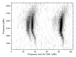
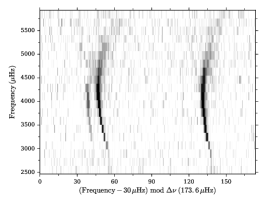
3.2.2 Prior functions
For mode frequencies, we adopted wide top-hat priors centered on the initial guesses of the frequencies. Top-hat priors were also adopted for the rotational frequency splitting and inclination , with the inclination sampled from the range to . The reason for the extended range in inclination is that if the solution is close to either or any sharp truncation from a prior at these values will make it difficult to properly sample these extreme values. The final posterior on the inclination was then obtained from folding the samples onto the range from to .
For the amplitudes and line widths we adopted a modified Jeffrey’s prior, given as (see, e.g., Handberg & Campante 2011)
| (3.11) |
which behaves as a uniform prior when and a standard scale invariant Jeffrey’s prior when . The maximum of the prior occurs at .
For mode visibilities we adopted truncated Gaussian functions as priors, defined as:
| (3.12) |
with given as:
| (3.13) |
Here, denotes the error function, and give the chosen mode value and width of the Gaussian, and and give the lower and upper truncations of the Gaussian. We specifically adopted for , for , and for . Similarly, we adopted truncated Gaussian priors for the parameters of the background. Here we used as the Gaussian mode value () the median of the posteriors from the background-only fit (see Section 3.2.1), and we adopted , , and .
To ensure that the mode identification did not swap for neighboring and modes, which is a risk especially at high frequency where the small frequency separation is small compared to the mode line width, we added the prior constraint that on that it must be positive. In principle could be negative in the event of bumped modes, however, because the stars were screened for bumped modes and the strength of an avoided crossing is expected to be lower than that of a mode due to the larger evanescent region (see, e.g., Aerts et al. 2010; Deheuvels & Michel 2011), we do not expect values of for these stars.
3.2.3 Quality assurance
For each fitted mode, we computed a metric for the quality of the fit in the same manner as detailed in Davies et al. (2016), see also Appourchaux (2004) and Appourchaux et al. (2012a). Briefly, we first ran a fast null hypothesis () test to identify which modes had an unambiguous detection, and for which the probability of detection conditioned on the data needed to be explicitly determined and evaluated. This was done because the explicit determination of is computationally expensive. In the fast test it was assessed whether the S/N in the background corrected power spectrum () for a given proposed mode, with the power binned across a number of frequencies to account for the spread in power from the mode line width, was consistent with a pure noise spectrum or whether the hypothesis could be rejected at the level (Appourchaux 2003a, 2004; Lund et al. 2012). When the high S/N modes had been identified in this manner the probability of detection was computed for the remainder low-S/N modes.
In the computation of both the probability of assuming , , and the probability of the alternative hypothesis of a detected mode, , need to be estimated. The latter was assessed by integrating the probability of measuring the data given a model over a range of mode parameters — this integration was achieved by marginalizing over , with the parameter space sampled over the posteriors from the peak-bagging using emcee. Specifically, a mixture-model was used in which both and were optimized simultaneously to give , the probability of observing the data given the model of a given set of modes with parameters :
| (3.14) |
Here, the parameter , ranging between 0 and 1, then gives the probability of the detection of the given set of modes. This probability was kept free in the emcee run, and in the end was assessed from the posterior distribution of (Hogg et al. 2010; Farr et al. 2015). We finally report the Bayes factor , given as the median of the posterior probability distributions of the natural logarithm of the ratio of over , as:
| (3.15) |
The value of can then be assessed qualitatively on the Kass & Raftery (1995) scale as follows:
For a detailed account of the quality control we refer to Davies et al. (2016).
3.3. Derived quantities and correlations
Besides the parameters included in the model of the power spectrum, we computed parameters for derived quantities, such as frequency difference ratios. Firstly, we derived the frequency ratios defined as (Roxburgh & Vorontsov 2003)
| (3.16) | ||||
Here, and are the smooth five-point small frequency separations defined as
| (3.17) | ||||
| (3.18) |
and the large separation is
| (3.19) |
These ratios are useful for model fitting, where they can be used instead of individual frequencies (Lebreton & Goupil 2014; Silva Aguirre et al. 2015) because they are largely insensitive to the stellar surface layers (Kjeldsen et al. 2008a; Ball & Gizon 2014; Roxburgh 2015; Ball et al. 2016). For further details on the use of these ratios we refer to Roxburgh & Vorontsov (2003, 2013), Roxburgh (2005), Otí Floranes et al. (2005), and Silva Aguirre et al. (2011, 2013).
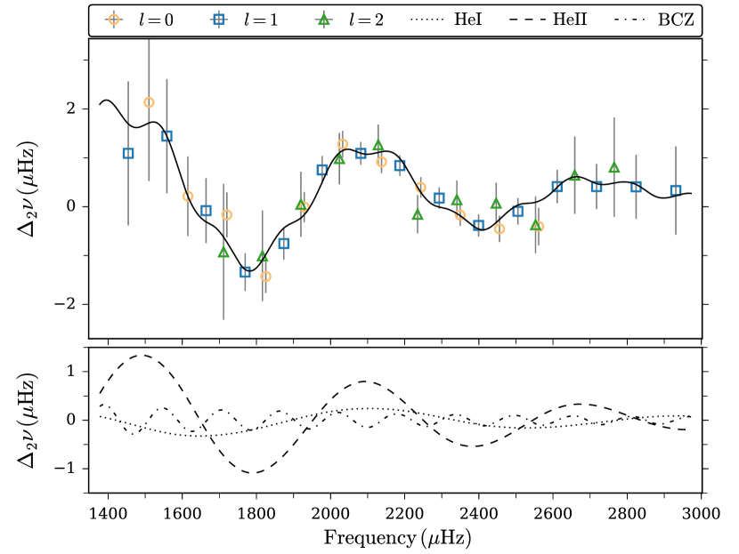
Secondly, we calculated the second differences:
| (3.20) |
which are useful for studying acoustic glitches from the base of the convection zone and the position of the second helium ionization zone (see, e.g., Basu et al. 1994, 2004; Houdek & Gough 2007; Mazumdar et al. 2014). Figure 5 gives an example of the second differences for KIC 6225718 (Saxo2), together with the best-fitting glitch model from Houdek et al. (in prep.). The second differences shown in Figure 5 were computed using Equation 3.20 on the frequencies given in Table 6, and frequency uncertainties were taken as the average of the asymmetric uncertainties.
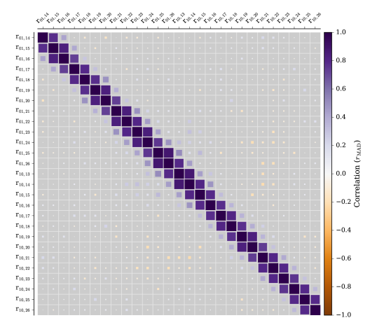
In computing these derived quantities we used the full posterior probability distributions (PPDs) of the individual frequencies entering in the descriptions, rather than using simply the median value for the PPD of a given frequency. This ensured that any asymmetries, and deviations from a Gaussian shape in general, that might be for the PPDs of the individual frequencies were properly propagated to the description of the derived quantity. The final value and credible interval were then computed from the distribution of the quantity in the same manner as for the parameters describing the model power spectrum. Using the full distribution also allowed us to easily compute the correlations between the above frequency differences and ratios, such that these might be included as a covariance matrix in any fit to the quantities.
The parameter correlations were calculated in a robust way using the median absolute deviation (MAD) correlation coefficient (see Pasman & Shevlyakov 1987; Shevlyakov & Smirnov 2011). The MAD estimator is given by the median of the absolute deviation around the median. We opted for instead of the standard Pearson product-moment correlation coefficient, because the latter would be very susceptible to even a single walker in the MCMC optimization straying away from the stationary solution. The between two parameters and was calculated as follows:
| (3.21) |
where and are the robust principle variables for and :
| (3.22) | ||||
| (3.23) |
4. Results
Below we present some of the conclusions that can be drawn on the different parameters extracted from the peak-bagging. Results on the rotational splittings and inclination angles will be presented in a separate paper. All results will be made available on the KASOC database\@footnotemark.
4.1. Mode frequencies
4.1.1 Frequency uncertainties
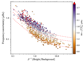
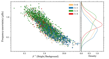
A proper understanding of the uncertainties on mode frequencies is important, because they will ultimately limit the precision with which stellar parameters can be estimated from modeling the individual frequencies. We may compare the frequency uncertainties from the peak-bagging with expectations from an analytical maximum likelihood (ML) approach (see, e.g., Libbrecht 1992; Toutain & Appourchaux 1994; Ballot et al. 2008). It should be noted that the ML estimator (if unbiased) reaches the minimum variance bound, in accordance with the Cramér-Rao theorem (Cramér 1946; Rao 1945). Thus one should expect uncertainties at least as large as those from the ML estimator (MLE). The standard way of obtaining uncertainties on a ML estimator is from inverting the negative Hessian matrix, and therefore the standard parameters come from the diagonal elements of the resulting variance-covariance matrix. The Hessian itself is obtained from the matrix of second derivatives of the log-likelihood function with respect to the parameters. Assuming an isolated mode as described by Equation 3.1 and a likelihood function as given in Equation 3.9, one may follow Libbrecht (1992) and Toutain & Appourchaux (1994) in defining a theoretical Hessian corresponding to the average of a large number of realizations. From this, the predicted frequency uncertainty for an isolated mode of a given is given as (Ballot et al. 2008):
| (4.1) |
where (the noise-to-signal ratio) is the level of the background divided by the mode height; gives the stellar inclination; is the reduced splitting, given by ; and is the observing duration. For radial modes () the factor only depends on and is given by (Libbrecht 1992):
| (4.2) |
For the general version of , see Ballot et al. (2008).
In Figure 7 we show the individual frequency uncertainties obtained from the peak-bagging as a function of , i.e., the signal-to-noise ratio of the mode. The left panel shows the behavior for the radial () modes. We see that the uncertainties for a given value of depend on as expected from Equation 4.2, and for a given a clear dependence is seen as a function of . Given the relatively small spread in , the vertical gradient largely depicts the gradient in and, as expected, the largest values of are seen towards low values because of the correlation between and mode heights. Comparing with Equation 4.1, we find that the median uncertainties from our MCMC peak-bagging are times larger than those predicted from the ML estimator.
The right panel of Figure 7 shows the uncertainties for all extracted modes. The uncertainties for each angular degree again follow the expected trend against . Some extra scatter is expected from and , but overall the modes are seen to follow the trend of the ones. The kernel density estimates of the uncertainties for a given , obtained by representing each sample with a Gaussian kernel, show that the uncertainties of dipole () modes are overall the lowest, followed by and . This is expected because (Equation 3.2), hence modes will typically have the highest S/N. The are seen not to follow this trend, probably because only the very highest amplitude were selected for fitting.
It is reassuring to see that the measured uncertainties follow expectations to this level, also considering that Equation 4.1 is constructed for an isolated mode without factoring in potential contributions from close-by neighboring modes. We note that the demonstration of the agreement is useful for predicting uncertainty yields for future missions like TESS (Ricker et al. 2014) and PLATO (Rauer et al. 2013), and could potentially be used to adjust uncertainties derived from a much faster MLE fitting (see, e.g., Appourchaux et al. 2012a) in cases where the sheer number of stars investigated would render the relatively slow MCMC approach impractical.
4.1.2 Average seismic parameters
| KIC | |||||||||
|---|---|---|---|---|---|---|---|---|---|
For each star we computed the average seismic parameters, including and , from the mode frequencies (see Table 2). The value of was obtained by fitting a Gaussian function to the extracted amplitudes as a function of frequency. The value found for the solar of is in agreement with the value of by Huber et al. (2011). We obtained and from a fit to the extracted mode frequencies with an extended version of the asymptotic relation, as in Lund et al. (2014a) (see also Mosser et al. 2011, 2013). This fit was made in a Bayesian manner using emcee, with a likelihood function assuming Gaussian frequency errors, and with final parameter values and uncertainties given by the posterior medians and HPDs. We initially adopted the following formula:
| (4.3) | ||||
Here gives the value of the large separation at . The latter corresponds to the radial order , which may take on a non-integer value. Specifically, is obtained for a given from interpolating the measured mode frequencies () against radial order () to the frequency of . This description gives a direct estimate of, for instance, the small frequency separations , given as the amount by which modes are offset from the the neighboring modes (), and (see, e.g., Bedding 2011). The value of is a good probe of the evolutionary state of the star because it is sensitive to the sound-speed gradient of the core, which in turn varies with the composition. The frequency dependence of these frequency separations is captured by the change in , assumed to change linearly with (or frequency), as found, for instance, for the Sun by Elsworth et al. (1990) (see also Toutain & Fröehlich 1992; Anguera Gubau et al. 1992). Lastly, the change in the large separation, assumed quadratic in , is included and mimics the overall curvature of the ridges in the échelle diagram.
We found this description to perform poorly across the range of stars in the sample, which is to be expected for more evolved stars (see, e.g., Gabriel 1989; Christensen-Dalsgaard 1991). To that end we modified the formula as follows:
| (4.4) | ||||
where the term has been replaced by , which takes on independent values for . Thereby we optimize independently for the separations and . In the fit we also included with a Gaussian prior from the fit to the mode amplitudes; the values of , , and correlate strongly, but we include to properly marginalize over the uncertainty of the pivoting . Figure 8 gives an example of the fit of Equation 4.4 to KIC 8228742 (Horace). All parameters from the fits are listed in Table 2.
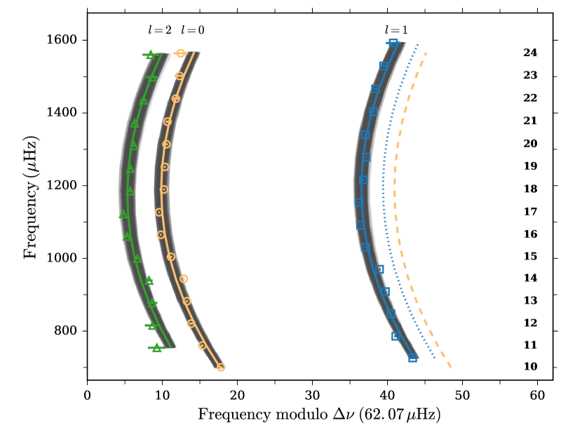
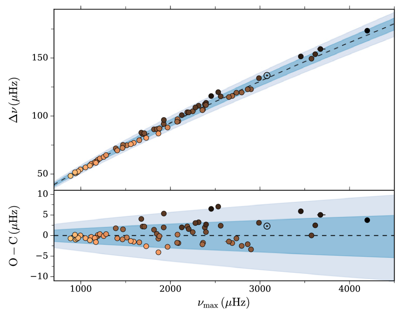
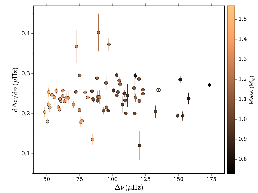
Figure 9 shows the estimated values for vs. , together with the empirical relation by Huber et al. (2011), with which we find an excellent agreement. We can even see the expected mass gradient in the residuals, with higher mass stars having slightly lower for a given . Also shown is the change in the large separation, which is found to be near-constant at and thus always with the same concavity sign, corresponding to a positive gradient of the large separation with frequency. Here one should remember that a constant value of against would correspond to a linear change in with frequency.
For the Sun we obtain a value of of ; comparing this to the value of by Huber et al. (2011) we would expect a slightly smaller value, because the curvature is incorporated in our estimation. However, the value of by Toutain & Fröehlich (1992), who also used a second-order version of the asymptotic relation, compares very well to our estimate.
The estimated values of have already been shown in Figure 3. For the estimation of it should be noted that this value is strongly anti-correlated with , and a small change in can thus induce a significant change in (White et al. 2011b). This will especially take effect if the estimate of is off, because defines the pivoting point for the change in , , and the curvatures. Like White et al. (2011b), we see an offset between the estimated and those obtained from model tracks, which is ascribed to the effects of the incorrect modeling of the stellar surface layers. In Figure 3 we show the -tracks adopted from White et al. (2011a), which were computed from evolutionary tracks from the Aarhus STellar Evolution Code (ASTEC; Christensen-Dalsgaard 2008), neglecting diffusion and core overshoot and with . It should also be noted that the from models were derived in a slightly different manner than used here, as described by White et al. (2011a). We therefore also estimated the values for and using the White et al. (2011a) method, namely from a weighted fit of the asymptotic function in Equation 3.10 to the radial mode frequencies as a function of radial order , and with weights given by a Gaussian with a FWHM of . Comparing the values for and from the fit of Equation 3.10 versus Equation 4.4 we only find minor differences in estimated values. For the maximum absolute difference was , with no systematic differences; for a maximum difference of was found, and again with no systematic differences.
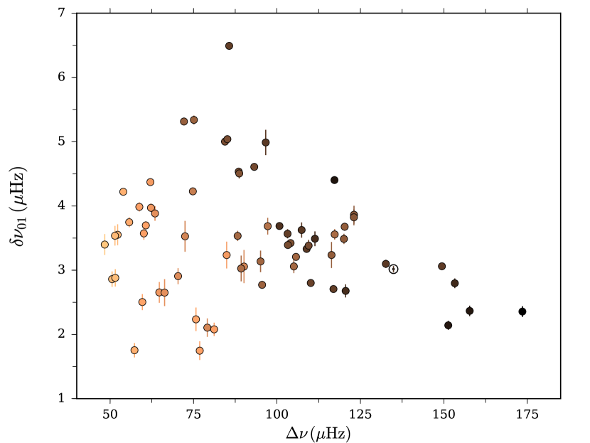
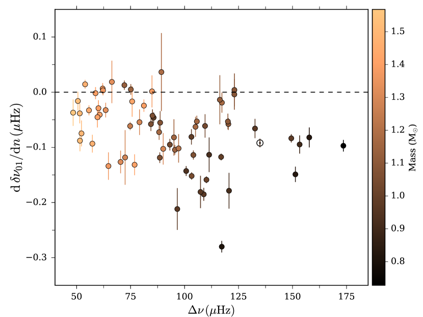
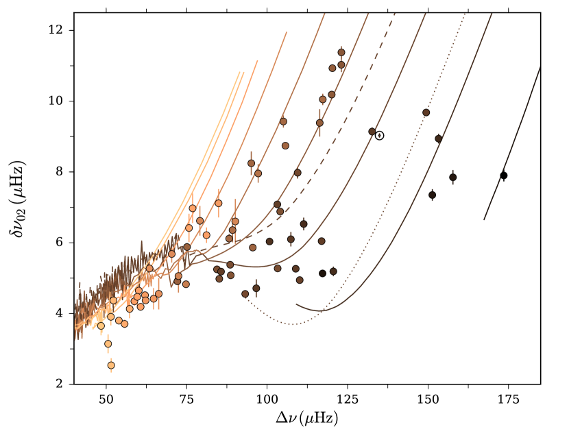
In Figures 10 and 11 we show the estimated values for the separations and , together with their gradients in (or frequency); the results for in Figure 11 are given in the form of a modified C-D diagram (see Christensen-Dalsgaard 1993; White et al. 2011b, a, 2012). Because all values for the changes in and are either zero or negative, we see that the small separations are virtually all decreasing functions of frequency. In Figure 11 we show again the ASTEC tracks from White et al. (2011a). It is interesting to see the degree to which the asymptotic relations to first (Equation 3.10) and second (Equation 4.3) order are satisfied. From these one would expect a ratio of from assuming – in Figure 12 we show this ratio for the sample.
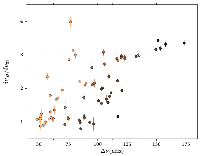
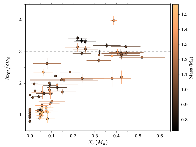
As seen, only a few stars, including the Sun, actually adhere to the expectation from the asymptotic relation. This was similarly found by Christensen-Dalsgaard & Houdek (2010)777expressed in the units and . for Cen A (Bedding et al. 2004), while Cen B (Kjeldsen et al. 2005) was found to fulfill the asymptotic relation. As explained by Christensen-Dalsgaard & Houdek (2010) this reflects a rapid variation of the sound speed in the core of Cen A from its more evolved state due to its higher mass compared to the B component. Similarly, Verma et al. (2014) found an increasing departure from the asymptotic description of the oscillation frequencies while fitting the signatures of the acoustic glitches. The departure becomes noticeable when a peak in the Brunt-Väisälä frequency develops just outside the stellar core towards the end of the MS and becomes comparable or higher than the lowest frequency fitted. To check this evolutionary explanation, we plot in the right panel of Figure 12 the against the central hydrogen content , because this serves as a good probe for the evolutionary state. As seen, stars with high , i.e., stars that are less evolved, adhere better to the asymptotic regime than the evolved stars with low . The values of were obtained as part of the modeling with the BASTA pipeline; we refer to Paper II for further details. While a difference from a ratio of can be explained from an evolutionary viewpoint, it is interesting to note that the majority of the stars analyzed indeed do not follow the asymptotic relation. This is a cautionary note to the use of Equation 3.10 and/or Equation 4.3 for extracting average seismic parameters as here, or if used for predicting the location of oscillation modes frequencies in the power spectrum from measured in an independent manner. For details on the physics behind the curvatures we refer to Tassoul (1980); Houdek & Gough (2007); Cunha & Metcalfe (2007), and Mosser et al. (2013) and references therein.
4.2. Mode amplitudes
| KIC | ||||||||||
|---|---|---|---|---|---|---|---|---|---|---|
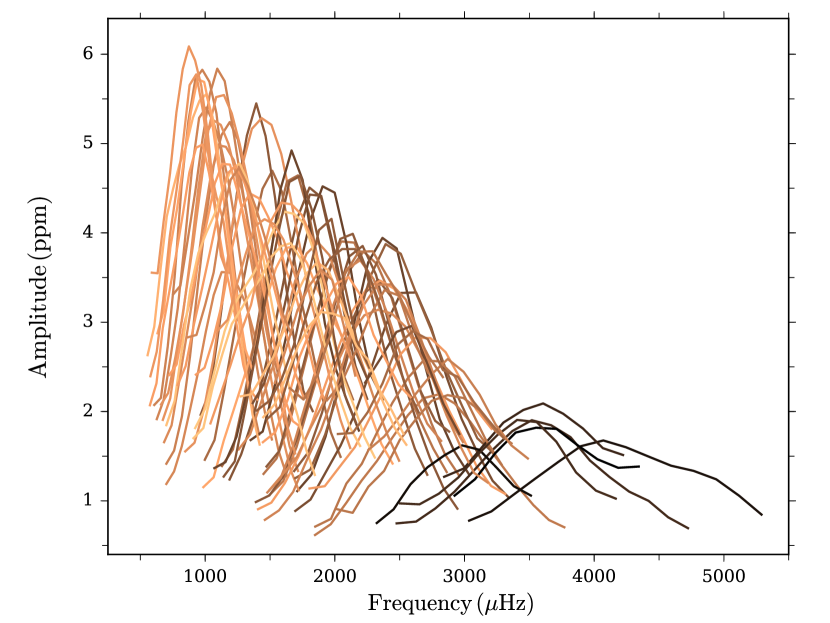
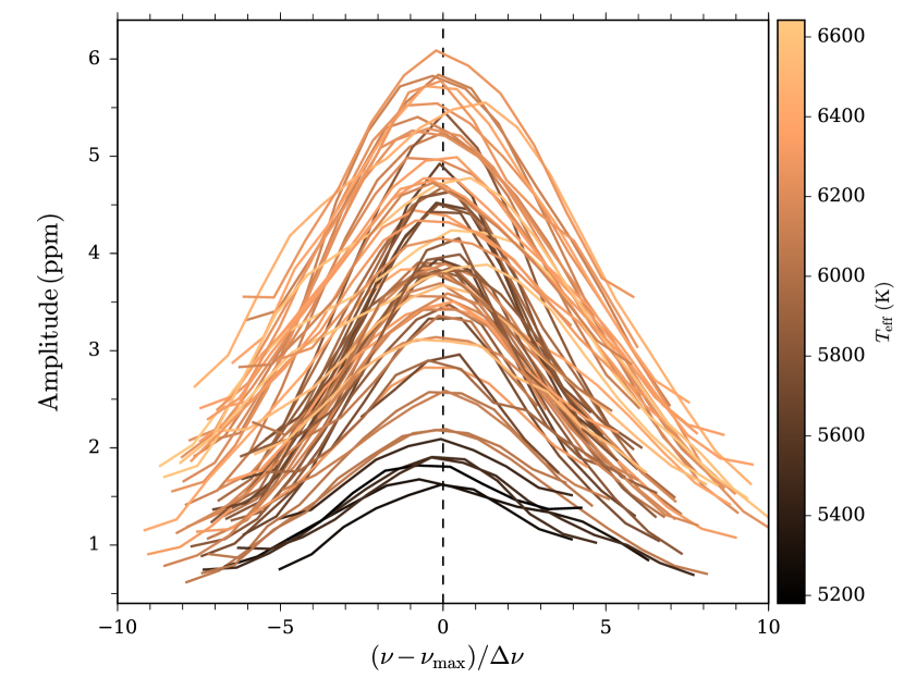
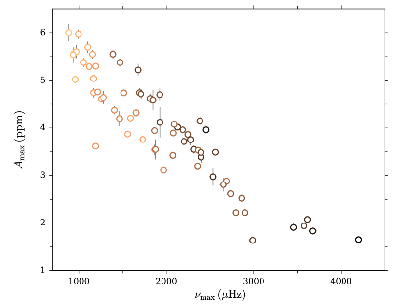
Mode amplitudes were measured in the peak-bagging as described in Section 3.1. Figure 13 displays the radial degree 5-point Epanechnikov (Epanechnikov 1969; Hastie et al. 2009) smoothed amplitudes for all the stars in the sample against frequency (left) and normalized against distance from (right). One clearly sees the overall decrease in amplitude with increasing (Kjeldsen et al. 2005; Arentoft et al. 2008), and thus decreasing (Kjeldsen & Bedding 1995, 2011; Appourchaux et al. 2014a).
The value of was estimated from the amplitudes as the frequency where the modes of oscillation show their maximum amplitude, .
Figure 14 gives the measured values for against (Table 3). We see both the expected change with , in addition to a mass gradient across the overall decrease in with (Huber et al. 2011).
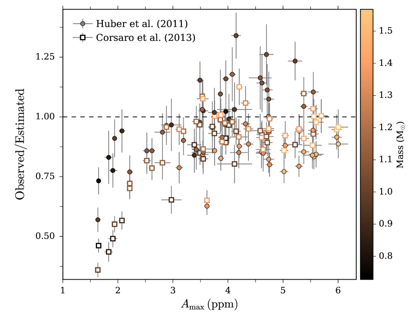
In Figure 14 we also give a comparison to the amplitudes estimated from the scaling relations of Huber et al. (2011):
| (4.5) |
with , , and and Corsaro et al. (2013):
|
|
(4.6) |
with , , , and . In converting the bolometric amplitudes from these relations to the Kepler bandpass we used the root-mean-square value of from Michel et al. (2009) and the temperature dependent bolometric correction by Ballot et al. (2011), which is specific to the Kepler spectral response function. Overall we see a reasonable agreement with a scatter within approximately as also found by Huber et al. (2011). At low amplitudes the Huber et al. (2011) relation is seen to provide the best agreement, while the Corsaro et al. (2013) relation has an overall lower scatter across the amplitude range. We note that the relations tested here were calibrated against values obtained using the method of Kjeldsen et al. (2005, 2008b) and the high range occupied by the stars in the current analysis is sparsely covered in the calibrations of the scaling relations, so a better relationship than observed cannot readily be expected (see more below). In addition, amplitudes will have natural scatter due to the impact of activity (Chaplin et al. 2011b).
4.2.1 Amplitudes from smoothed amplitude spectra
With amplitudes measured from individual modes it is interesting to see how these compare to those obtained from the often adopted method by Kjeldsen et al. (2005, 2008b). This is especially worthwhile because it is often amplitudes from this method that are extracted by automated analysis pipelines (see, e.g., Huber et al. 2009; Hekker et al. 2010; Mathur et al. 2010), and thus used in calibrating scaling relations (see, e.g., Stello et al. 2011; Huber et al. 2011; Corsaro et al. 2013).
Amplitudes were estimated following the prescription of Kjeldsen et al. (2008b). Here the power density spectrum is first convolved with a Gaussian filter with a FWHM of , to produce a spectrum with a single power hump from the oscillations. A noise background is then fitted to the smoothed spectrum and subtracted, after which the spectrum is multiplied by and the square-root is taken to convert to amplitude. The multiplication of converts to power per radial mode, with giving the effective number of radial modes per order, i.e., (see Equation 3.2). Concerning the order of the different steps in the method we subtract instead first the fitted background function from the peak-bagging, and then apply the smoothing — this removes the potential bias on both the amplitude and central frequency of the smoothed power hump from mixing background and oscillation power, and then try to fit the now smoothed underlying background with a non-smoothed background function.
The value of is often kept fixed rather than estimated for a given star following, for instance, the results by Ballot et al. (2011). Bedding et al. (2010) estimated a value of for the Sun as seen by Kepler using the method of Bedding et al. (1996) and Kjeldsen et al. (2008b) and adopting a mean observing wavelength of — this value has since been used by, e.g., Stello et al. (2011), Huber et al. (2011), and Corsaro et al. (2013). In our estimation of amplitudes we tried both the value of and the one obtained from the visibilities measured in the peak-bagging .
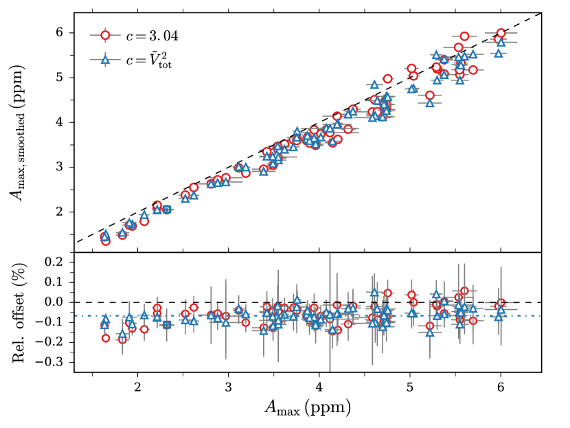
Figure 15 shows the result from this exercise; we find that the values from the above method are systematically offset (fixed bias) from those estimated from individual frequencies, with a median relative offset of ; no proportional bias is seen. This offset could in part originate from the somewhat arbitrary choice of for the smoothing window — however, if this was the only contributor one might expect a proportional offset rather than a constant one. The identified offset fully corroborates the results by Verner et al. (2011) who found a systematic offset between and from pipeline analysis of simulated data. We observe the same median offset for the different values of , but the scatter is slightly lower for the values using from the measured visibilities. Considering that and thus depends on various stellar parameters, such as , , and , it should be expected that adopting a constant adds to the scatter. The values of from the smoothing method, with both values of are given in Table 3.
4.3. Mode line widths
Following Appourchaux et al. (2014a) we adopt the following relation for the line widths against mode frequency:
| (4.7) |
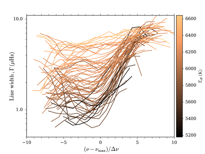
where the first part describes a power law trend with an exponent and a value of at . The second part describes a Lorentzian dip in the line widths in , centered on with a width and an depth . For the fit the values of were calculated from the posterior distributions; the -distribution is typically better approximated by a normal distribution (Toutain & Appourchaux 1994). We note that while Equation 4.7 matches that reported by Appourchaux et al. (2014a), these authors did in fact use a formula with the Lorentzian subtracted rather than added as in Equation 4.7 (Appourchaux et al. 2016). Both formulations can be used, but the reported parameters will naturally differ; in Equation 4.7 is for instance constrained to a value between 0 and 1 if a dip in is to be produced, whereas it can take on any value above 1 if the Lorentzian is instead subtracted. We chose the formulation where the Lorentzian is added in log-space, because we found that this provided better constrained fits from a lower correlation between the , , and parameters. We note that the parameter has two solutions, one higher than , and one lower — in our fits we chose the solution with a prior on . All stars were fitted using both the full version of Equation 4.7 and using only the first power law component — Figure 16 shows for all stars in the sample the measured line widths against a proxy for the radial order. The fit was made using emcee (Foreman-Mackey et al. 2013), with the parameter values and uncertainties given by the posterior distribution medians and HPD intervals. We evaluate which of the two types of fit is the best based on a visual inspection of the fits.
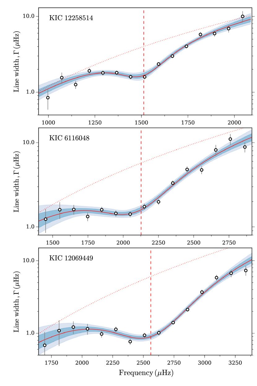
Figure 17 shows three examples where the full version of Equation 4.7 was deemed the better — as seen the line widths show a clear depression around . We omitted fitting the solar line widths from the degraded VIRGO data, because in computing relations for the fit parameters we are interested in as accurate and precise data as possible.
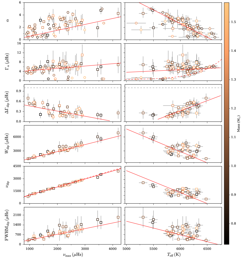
The parameters from the fits are given in Table 3 and shown in Figure 19 as a function of and . For the dependencies of the FWHM of the Lorentzian line width dip in frequency units we used the transformation (Appourchaux et al. 2016). The amplitude of the Lorentzian dip may be calculated using the transformation 888Note that this , where the Lorentzian in Equation 4.7 is added rather than subtracted, is different from that given by Appourchaux et al. (2014a) who instead has .. Like Appourchaux et al. (2014a) for their sample of 22 Kepler stars, we find a clear correlation between the Lorentzian width ( or ) and , while the power law exponent () and the dip amplitude () are found to correlate most strongly with . Only for the fits without the Lorentzian component does the value of correspond to the line width at , which is seen to correlate with . We return to the overall behavior of the line width at against below. Our estimates of agree well with updated values from Appourchaux et al. (2016). We make linear fits to the different parameters () against as and as . Specifically, we perform a Deming regression (Deming 1943) where uncertainties in both the dependent () and independent variables () are considered via the following merit function (Press et al. 1993):
| (4.8) |
which serves as our log-likelihood function in the emcee optimization. The coefficients from the different fits are given in Table 4. For the fit of against we include only the values from the fit including the Lorentzian in Equation 4.7. Some of the scatter in the relations will likely be due to activity; the dip in line widths for the Sun has for instance been found to depend on the solar cycle (see, e.g., Komm et al. 2000a, b). We note that the fit coefficients in Table 4 may well be used to define prior functions and initial guesses in future peak-bagging exercises.
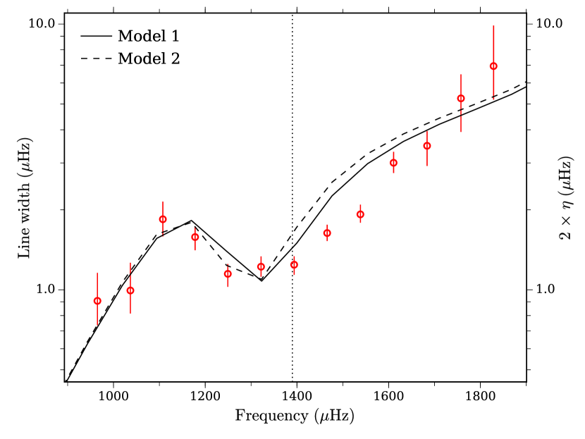
For a star with a temperature of the Sun we find that it should have an exponent of — this comes close to that measured by Komm et al. (2000b) of for frequencies below , which is about the lower limit of what one would observe for a similar star with Kepler. In general the exponent for the Sun has been measured below the dip where higher values have been found, e.g., by Libbrecht & Woodard (1991), by Chaplin et al. (1997), and by Davies et al. (2014a) — it is therefore not surprising that a lower value of is found when the measurement is done across the dip. Like Appourchaux et al. (2014a) we find that the amplitude of the line width dip decreases with . This behavior is contrary to theoretical damping-rate estimates (Balmforth 1992; Houdek 1996) which assume solar-calibrated convection parameters, such as the mixing-length and anisotropy of the turbulent velocity field, for damping-rate calculations in other stars. Updated calculations of mode damping rates (Houdek et al., in prep.) are, however, able to capture the overall behavior of the line widths for stars in the current study spanning a large range in – these new calculations adopt, in addition to the standard ingredients described in Houdek et al. (1999) and Houdek (2006), turbulent pressure profiles and relations calibrated to 3D hydrodynamical simulation results by Trampedach et al. (2014). An example of such an improved damping-rate computation provides Figure 18, which compares estimated mode line widths with observations for KIC 6933899 (Fred), using stellar parameters from the best fitting ASTFIT model (Paper II).
The estimate of at was obtained by a Monte Carlo sampling from the posteriors of the fit parameters in Equation 4.7 and the estimate of from the mode amplitudes. The values obtained are plotted against in Figure 20 and given in Table 3. We have fitted two relations for the line width at , namely, the power-law relation by Appourchaux et al. (2012b):
| (4.9) |
and the exponential relation used, for instance, by Corsaro et al. (2012):
| (4.10) |
In the fits of Equations 4.9 and 4.10 we complement our set of line widths with those from peak-bagging of 42 giants in NGC 6819 by Handberg et al. (2016, submitted) where we adopt an uncertainty of on for all stars, and 19 red giants by Corsaro et al. (2015) where we adopt values from Pinsonneault et al. (2012) (from the infra-red flux method). The line widths from Handberg et al. (2016, submitted) are given by the average of the radial modes; those from Corsaro et al. (2015) are given as the average over three radial modes centered in the mode with the highest amplitude.
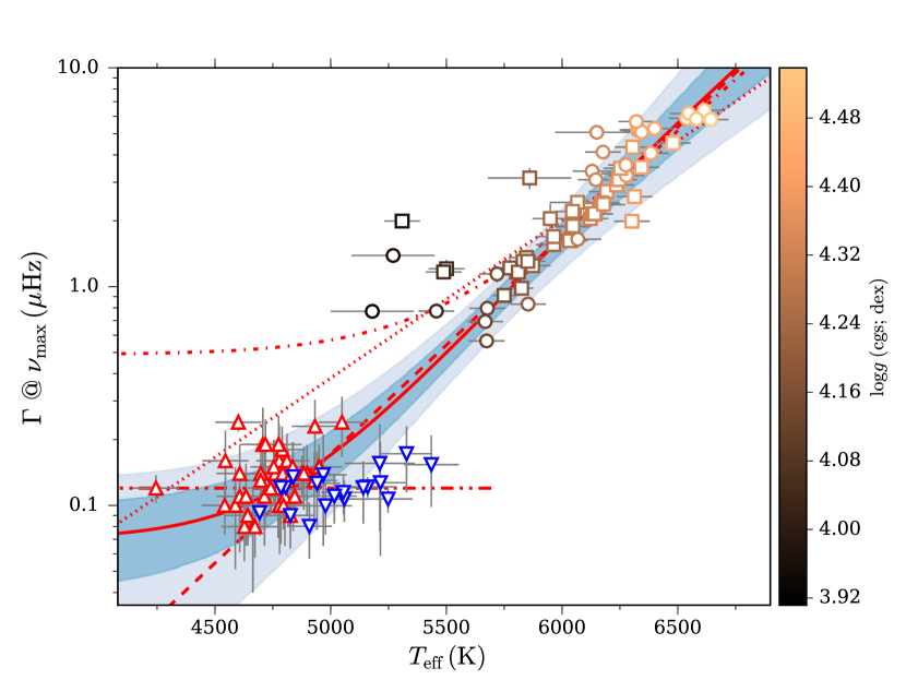
We fit both relations to the line widths using an orthogonal distance regression (ODR; Boggs & Rogers 1990) in order to take into account both the uncertainties on and . This procedure is employed in a Monte Carlo (MC) run where we in each iteration draw at random 50 stars to include in the fit. For Equation 4.9 we obtain from the MC distributions the following values for the fitting parameters: , , and ; for Equation 4.10 we obtain: and . If we fit only the red giants by a constant value for the line width we find a value of . For the parameter uncertainties we have added in quadrature the median from the internal uncertainties from the ODR and the standardized MAD of the best fit ODR values from the MC run. We note here that neglecting the uncertainties in from using, for instance, an ordinary least squares (OLS) approach will affect the fit and the parameters in Equation 4.9. Both relations perform reasonably well, but the fit of Equation 4.9 gives a slightly lower value. The resulting relations are displayed in Figure 20. Also shown in Figure 20 are the fits obtained by Appourchaux et al. (2012b) (parameters from their Table 3) and Corsaro et al. (2012).
We see that the cooler MS targets appear to be outliers to the overall relation between line width and temperature. From Figure 19 we can see that the value of has a proportional bias with respect to , hence the higher the the further below does the dip in line widths appear. For Figure 20 the line widths were estimated at and thus away from the line width dip for the highest stars, it is therefore not surprising that these deviate from the overall relation. An offset could potentially also be caused by frequency shifts from stellar activity cycles (Chaplin et al. 2007, 2008a), the evidence of which is currently being studied by Santos et al. (in prep.). The line width for KIC 7970740 was omitted in the fits as it appears to be a particularly strong outlier at K.
We find that our estimates agree well with those from Appourchaux et al. (2012b) with the main difference seen at low temperatures where the fit is the least constrained if no line widths from giants are included. The estimates from Corsaro et al. (2012) appear to be higher at low temperatures than the line widths from Handberg et al. (2016, submitted) — this could be due to the method of estimating in Corsaro et al. (2012) from collapsed échelle diagrams for a group of stars. Some scatter is to be expected, because the line widths will depend on parameters besides — Belkacem et al. (2012, 2013) specifically suggest a scaling with and . As noted by Appourchaux et al. (2012b), the uncertainty on currently sets the limitations for obtaining a more well constrained prediction for at , which may then be confronted with theoretical calculations. As for the dip amplitude, activity and stellar cycles will play a role in the scatter around the mean relation for at (Komm et al. 2000b; Chaplin et al. 2008a). For other analysis of the variation of at we refer to Goldreich & Kumar (1991); Houdek et al. (1999); Chaplin et al. (2009); Baudin et al. (2011), and Belkacem et al. (2012, 2013).
4.4. Mode visibilities
| KIC | ||||
|---|---|---|---|---|
Mode visibilities are estimated as part of the peak-bagging (see Equation 3.2); these are given in Table 5. Figure 21 shows the obtained visibilities as a function of , , and mass. The total visibilities are computed from the combination of the MCMC chains for the individual visibilities. We see no strong correlation with , (not shown), or (not shown), and some scatter is observed for the visibilities about their median values. From median binned values there are slight indications of structure in the visibilities against the plotted parameters; the visibilities do, for instance, seem to peak around a temperature of and have a depression around a mass of . None of the dependencies are, however, very strong, but they do appear similar in shape for different angular degrees.
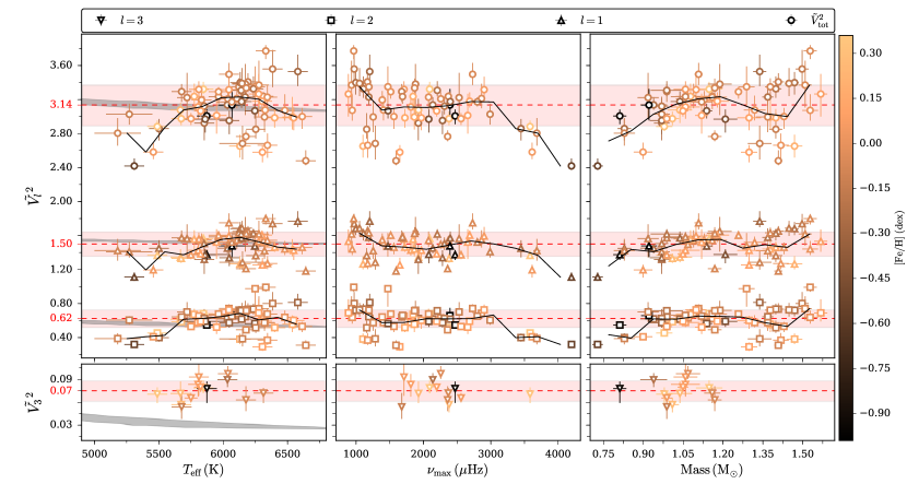
In comparing to the theoretically estimated values by Ballot et al. (2011), which are calculated considering the Kepler bandpass, we see that in median visibilities are lower than expected, those for and are larger than expected, and the total visibilities (up to ) are only slightly lower than expected. The difference is most pronounced for the modes. It is important to note that because visibilities have only been measured for a subset of stars, it might be that the remainder of the stars (with a S/N too low for a visual detection of modes) have visibilities in agreement with theory. The comparisons do, however, qualitatively match those obtained by Mosser et al. (2012) for giants observed by Kepler; the modes disagree most with theory in their results too. Similar discrepancies with theory have also been observed for individual CoRoT and Kepler targets analyzed by Deheuvels et al. (2010), Mathur et al. (2013), and Lund et al. (2014a), and the Sun by Salabert et al. (2011). Given these discrepancies we discourage the adoption of fixed mode visibilities in peak-bagging exercises. To assess which other parameters in the peak-bagging contribute the most to the uncertainties on the visibilities, and thus which parameters will be most affected by adopting fixed visibilities, we show in Figure 22 with a box-plot the correlations between the visibilities and the remainder of the fitted parameters. Correlations have been estimated using Spearman’s rank correlation (Spearman 1904) from the MCMC chains, because this better catches dependencies which are monotonic but not necessarily linear (as done in Pearson’s correlation; Pearson 1895).
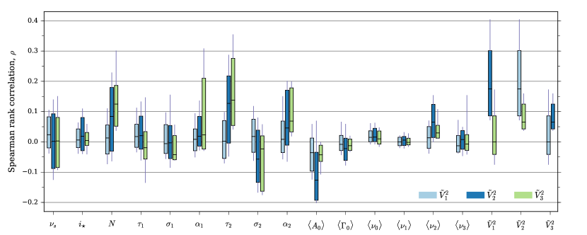
As seen, the correlations are overall quite small with median values within in all cases. The visibilities are seen to primarily correlate with the parameters of the noise background, as might be expected with an increasing correlation with increasing angular degree ; a small change in, say, has a relatively larger impact on the visibility of modes compared to that of modes and one should therefore expect a larger correlation. This suggests that fixing the visibilities might bias the fit of the background and vice versa for fixed backgrounds. One should however also be cautious with the extracted visibilities, because an inappropriate model for the background might bias the measured values.
Considering the total visibility we note that Ballot et al. (2011) include modes up to , but this should not significantly affect any observed discrepancy. The median value obtained for is , which is close to the value of (Bedding et al. 2010) often adopted in estimating radial mode amplitudes via the method of Kjeldsen et al. (2005, 2008b). In Section 4.2.1 we did indeed also find that the amplitudes from the smoothing method were equal in median from using and , with only a slightly reduced scatter from using the measured total visibility. The value of (or alternatively ) should therefore serve as a reasonably good choice for analysis of amplitudes for a large sample of stars, but the small systematic offset found in Section 4.2.1 should be remembered when comparing with theory. We note also that Mosser et al. (2012) find a mean value of from Kepler giants with between approximately 4000 and 5100 K, but with a larger scatter than for our values. This does, however, indicate that the visibilities do not increase with decreasing temperature as suggested by theory. If a trend exists with and/or , which should be the main parameters determining the visibilities, they cannot be clearly discerned from the observations.
Some of the discrepancies, and scatter in observed values, can likely be explained by some of the simplifications adopted in the calculations by Ballot et al. (2011) and in general. These include, for instance, the neglect of non-adiabatic effects and a height dependence on mode amplitudes in the stellar atmosphere (see, e.g., Baldner & Schou 2012; Schou 2014, 2015). Furthermore, phenomena such as spots and other local surface features will influence the measured visibility. An effect will also come from the way in which the stellar limb-darkening (LD) is described; the calculation of LD coefficients (LDCs) for parametrized LD laws will, e.g., depend on the description of convection in the adopted atmosphere models, the method used for integrating the specific flux, and the resolution used when fitting a parametrized LD law to these flux values. Ballot et al. (2011) compared their visibilities with those obtained using LDC from Sing (2010) (specific to the Kepler bandpass) and found that their values were generally higher. Similarly, Claret & Bloemen (2011) compared their Kepler LDCs to those of Sing (2010) and found differences. This indicates that some systematic uncertainty should be added to the theoretically derived visibilities. In any case Sing (2010) showed from fits to planetary transit curves that model computations of LDC generally disagree with those derived empirically. The treatment of the LD is, however, likely a secondary effect — as shown in Lund et al. (2014a) the specific LD law adopted (neglecting the linear one) only has minor effects on the visibilities, and the shape has to be changed by a large amount away from the limb in order to take effect. This, and the fact that discrepancies between measured and modeled visibilities are found for the Sun (Salabert et al. 2011), where the LD is well known as a function of wavelength (Neckel & Labs 1994), indicates that the simplified assumptions concerning the mode physics likely are the main contributor to the discrepancies. We note, however, that modes of would be relatively more affected by details of the LD, because of the considerably stronger cancellation for modes (total in the absence of LD), compared to modes of (Lund et al. 2014a). It could also be questioned if the assumption of equipartition of energy between modes of different angular degree holds true.
4.4.1 Detection of modes
For solar-like oscillators observed by Kepler the highest angular degree of modes is typically . Only for the highest S/N cases can higher degree modes be identified — in the current sample octupole modes were identified and included in the peak-bagging in 14 such targets. It is, however, possible to obtain information on the combined signal for modes in a given star. Such a signal could, for instance, be used in estimating the small separation which can contribute a constraint in modeling efforts (see, e.g., Bellinger et al. 2016).
To optimize the combined signal from modes of a given angular degree we applied the method outlined in Lund et al. (2014a). Briefly, the échelle diagram is collapsed along the vertical direction after having first stretched the frequency scale such that modes of a given form a straight ridge — this ensures that all mode power from the particular -values is co-added with as little spread as possible. Individual frequencies from best fitting ASTFIT models were used to stretch the frequency scale (see Paper II). Before the power is co-added the power spectrum is smoothed to account also for the mode line widths and a potential rotational splitting. In Figure 23 we show in a contour plot the collapsed échelle diagrams for all stars, optimized to increase the signal of modes. To further increase the visibility of these modes we first divided out the model of the power spectrum from the peak-bagging, including also fitted modes. We see that for most stars a clearly detectable signal from is present. It is beyond the scope of this paper to estimate for the stars and test the statistical significance of the signals, but Figure 23 should indicate that obtaining this information would be possible. Some of the signal seen around modes in the residual spectra is likely due contamination from higher degree modes () or deviations in the mode shape from the assumed simple Lorentzian — asymmetry of the modes would, for instance, leave some unaccounted for power in the residual spectrum.
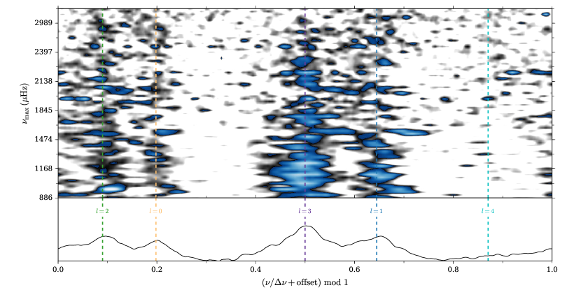
For the highest S/N targets one may further look for indications of hexadecapole modes.
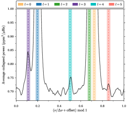
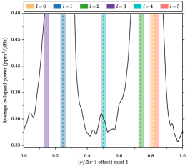
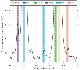
In Figure 24 we show the collapsed échelle diagrams optimized for the detection of for three targets with the strongest apparent signals, namely, KIC 6603624 (Saxo), KIC 7510397 (middle), and KIC 12069449 (16 Cyg B). As seen an excess in collapsed power in each of these cases falls close to the expected position at from the ASTFIT model. The signal seen in 16 Cyg A (not shown) and B corresponds well to the signal found in Lund et al. (2014a) from a shorter Kepler data set. Curiously, the peak around seen in Saxo and 16 Cyg B appears to coincide with the expected position of dotriacontapole modes — whether this signal truly is from modes requires further investigation. In any case, it is clear that for a star like KIC 7510397 the modes will be polluted by modes; similarly will modes pollute the signal, etc. (Appourchaux & Virgo Team 1998; Lund et al. 2014a).
5. Example output
For each of the 66 stars in the sample we have provided a set of outputs from the peak-bagging. Tables and plots for all stars will be available in the online appendices. The extracted parameters may in addition be obtained from the results section of the KASOC data base999http://kasoc.phys.au.dk/results/..
| 2.2 | |||||
| >6 | |||||
| >6 | |||||
| >6 | |||||
| >6 | |||||
| 1.45 | |||||
| >6 | |||||
| >6 | |||||
| 3.14 | |||||
| >6 | |||||
| >6 | |||||
| >6 | |||||
| >6 | |||||
| >6 | |||||
| >6 | |||||
| >6 | |||||
| >6 | |||||
| >6 | |||||
| >6 | |||||
| >6 | |||||
| >6 | |||||
| >6 | |||||
| >6 | |||||
| >6 | |||||
| >6 | |||||
| 3.01 | |||||
| >6 | |||||
| >6 | |||||
| >6 | |||||
| 3.94 | |||||
| >6 | |||||
| >6 | |||||
| >6 | |||||
| 3.66 | |||||
| >6 | |||||
| >6 | |||||
| >6 | |||||
| 3.12 | |||||
| >6 | |||||
| >6 | |||||
| >6 | |||||
| >6 | |||||
| >6 | |||||
| >6 | |||||
| >6 | |||||
| >6 | |||||
| >6 | |||||
| >6 | |||||
| 3.78 | |||||
| >6 | |||||
| >6 | |||||
| 1.45 | |||||
| >6 | |||||
| 4.92 | |||||
| 2.18 | |||||
| 3.81 | |||||
| 4.2 | |||||
| 1.22 | |||||
| 3.81 |
The outputs include first of all a table with the mode information from the MCMC peak-bagging, like the one given in Table 6 for KIC 6225718 (Saxo2). The table gives for a given mode the angular degree, radial order, frequency, amplitude, line width, and the natural logarithm of the Bayes factor from the quality control in Section 3.2.3. The uncertainties on the mode parameters are obtained from the HPD interval of the posterior probability distributions. As amplitudes and line widths are only fitted to radial modes we only give these values for these modes. The visibilities for a given star can be found in Table 5. We note that the radial orders given are obtained from matching to the expected value as a function of (see Section 3.2.1) — we suggest that this be used with some caution in modeling efforts and checked independently. A table is also included with the derived frequency difference ratios and second differences (see Section 3.3), examples of these are given in Tables 7 and 8.
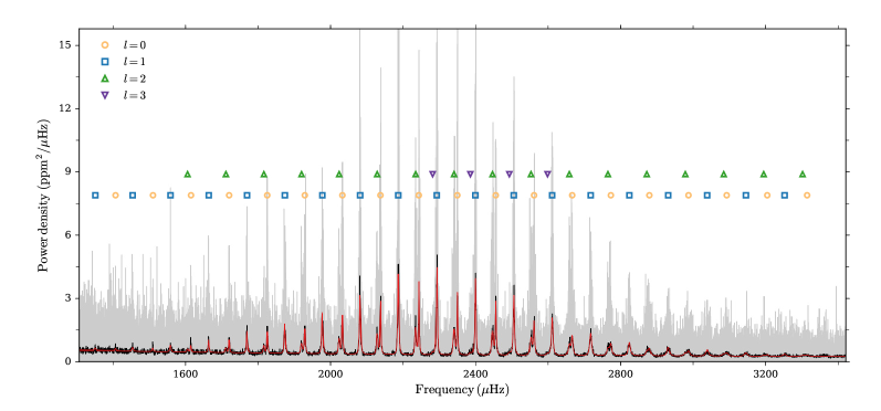
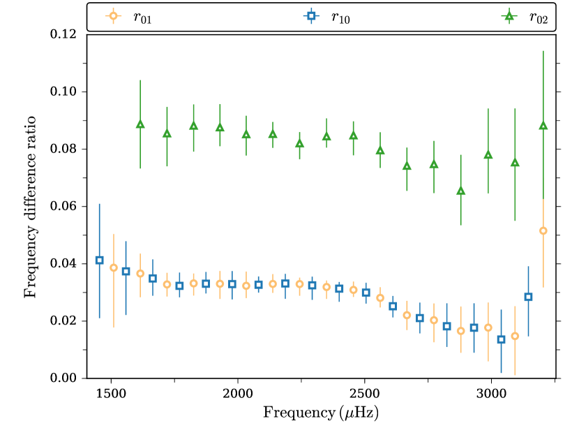
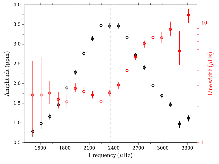
For each star a number of plots are also prepared. These include (1) a visualization of the obtained ‘best fit’ from the peak-bagging as in Figure 25, given by a plot of the power spectrum overlain with the best fit model and with an indication of the extracted modes; (2) an échelle diagram overlain with the extracted frequencies as in the left panel of Figure 26; (3) a plot of the derived frequency difference ratios as shown in the right panel of Figure 26; (4) a plot of the derived second differences as shown in Figure 5 for KIC 6225718 (Saxo2), but without model fits; (5) a plot of the extracted mode amplitudes and line widths as shown in Figure 27.
6. Conclusions
In this paper we have presented the mode parameters for a sample of 66 MS solar-like oscillators, the frequencies of which are modeled in Paper II. In addition to the individual mode frequencies we have constructed frequency difference ratios and their correlations for the use in modeling efforts. We also report for each star the values for the mode line widths, amplitudes, and visibilities. For each of these quantities we have derived summary parameters and descriptions, such as the average seismic parameters and and the behavior of mode line widths against frequency.
The reported parameters were derived through peak-bagging of the power spectra using an MCMC optimization scheme. This resulted in posterior probability distributions for each of the included parameters, from which credible intervals and correlations were directly obtained. We found that the derived frequency uncertainties adhere to the expectations from theory in terms of S/N, observing time, and line widths, and are only higher by a factor of compared to estimates from MLE. This observation will be useful for predicting seismic modeling yields for future missions such as TESS and PLATO. As a quality control on the detection of the reported modes, we performed a Bayesian hypothesis testing that for each mode gave the probability of detection (Davies et al. 2016; Appourchaux et al. 2012a). Our main conclusions are as follows:
-
The derived values for and agree with empirically derived relations from the Kepler mission. We derived parameters from an extended version of the standard asymptotic frequency relations, including mode ridge curvatures and variations of and small frequency separations. From the small frequency separations we further found that most stars deviate from the asymptotic description by an amount that correlates with the evolutionary state of the star, i.e., the central hydrogen content.
-
The measured amplitudes at for our sample largely follow the expected trend from empirical relations from Kepler. We also identified a systematic offset of approximately between the maximum amplitudes obtained from the modes and those obtained from the smoothing method by Kjeldsen et al. (2008b). This corroborates the findings by Verner et al. (2011). This systematic offset should be corrected for whenever the two methods are compared.
-
For the line widths we adopted the frequency dependence of Appourchaux et al. (2014a) given by an overall power law dependence and a Lorentzian dip near . We fitted this relation for all stars and were able to derive simple relations between the parameters of the fit and and . These were found to confirm the results by Appourchaux et al. (2014a). Such relations will be useful for future simulations of solar-like oscillators and may be compared to theory. We also obtained a fit for the dependence of the line width at , complementing our values with line widths from 42 giants in NGC 6819 (Handberg et al., submitted). The obtained dependence largely agreed with that found by Appourchaux et al. (2012b), except for stars with low .
-
Concerning the estimated mode visibilities, we found that those for were slightly lower than expected from the theoretical calculations by Ballot et al. (2011), whereas those for and were larger than expected, especially for the modes. We found no overall dependence on , which is also evident from the fact that Mosser et al. (2012) found a mean value of the total visibility at nearly the same level as here for Kepler giants, which have values lower by about K. Some structure was observed in the visibilities against and mass, but it was not possible to say directly if this is simply due to scatter from the measurements or if they have some underlying physical explanation. Applying the method of Lund et al. (2014a) enabled us to identify power from modes in most stars, and for some high S/N targets even for .
Acknowledgments
Funding for this Discovery mission is provided by NASA’s Science Mission Directorate. The authors acknowledge the dedicated team behind the Kepler and K2 missions, without whom this work would not have been possible. We thank Thierry Appourchaux for useful discussions on the properties of the line width fits, Ian Roxburgh for discussions on mode frequencies, and Enrico Corsaro for supplying line widths for a set of 19 red giants. We thank Jens Jessen-Hansen for inspiration to the paper title. Funding for the Stellar Astrophysics Centre (SAC) is provided by The Danish National Research Foundation (Grant DNRF106). The research was supported by the ASTERISK project (ASTERoseismic Investigations with SONG and Kepler) funded by the European Research Council (Grant agreement no.: 267864). MNL acknowledges the support of The Danish Council for Independent Research | Natural Science (Grant DFF-4181-00415). VSA and TRW acknowledges support from VILLUM FONDEN (research grant 10118). GRD and WJC acknowledge the support of the UK Science and Technology Facilities Council (STFC). SB is partially supported by NSF grant AST-1514676 and NASA grant NNX16A109G. DH acknowledges support by the Australian Research Council’s Discovery Projects funding scheme (project number DE140101364) and support by the National Aeronautics and Space Administration under Grant NNX14AB92G issued through the Kepler Participating Scientist Program. WHB acknowledges research funding by Deutsche Forschungsgemeinschaft (DFG) under grant SFB 963/1 “Astrophysical flow instabilities and turbulence” (Project A18).
References
- Aerts et al. (2010) Aerts, C., Christensen-Dalsgaard, J., & Kurtz, D. W. 2010, Asteroseismology, Astronomy and Astrophysics Library (Springer Netherlands)
- Andersen et al. (1994) Andersen, B. N., Leifsen, T. E., & Toutain, T. 1994, Sol. Phys., 152, 247
- Anderson et al. (1990) Anderson, E. R., Duvall, Jr., T. L., & Jefferies, S. M. 1990, ApJ, 364, 699
- Anguera Gubau et al. (1992) Anguera Gubau, M., Palle, P. L., Perez Hernandez, F., Regulo, C., & Roca Cortes, T. 1992, A&A, 255, 363
- Appourchaux (2003a) Appourchaux, T. 2003a, A&A, 412, 903
- Appourchaux (2003b) —. 2003b, Ap&SS, 284, 109
- Appourchaux (2004) —. 2004, A&A, 428, 1039
- Appourchaux & Virgo Team (1998) Appourchaux, T., & Virgo Team. 1998, in ESA Special Publication, Vol. 418, Structure and Dynamics of the Interior of the Sun and Sun-like Stars, ed. S. Korzennik, 99
- Appourchaux et al. (2012a) Appourchaux, T., Chaplin, W. J., García, R. A., et al. 2012a, A&A, 543, A54
- Appourchaux et al. (2012b) Appourchaux, T., Benomar, O., Gruberbauer, M., et al. 2012b, A&A, 537, A134
- Appourchaux et al. (2014a) Appourchaux, T., Antia, H. M., Benomar, O., et al. 2014a, A&A, 566, A20
- Appourchaux et al. (2014b) —. 2014b, ArXiv e-prints 1403.7046
- Appourchaux et al. (2016) —. 2016, A&A, 595, C2
- Arentoft et al. (2008) Arentoft, T., Kjeldsen, H., Bedding, T. R., et al. 2008, ApJ, 687, 1180
- Baglin et al. (2009) Baglin, A., Auvergne, M., Barge, P., et al. 2009, in IAU Symposium, Vol. 253, IAU Symposium, ed. F. Pont, D. Sasselov, & M. J. Holman, 71–81
- Baldner & Schou (2012) Baldner, C. S., & Schou, J. 2012, ApJ, 760, L1
- Ball et al. (2016) Ball, W. H., Beeck, B., Cameron, R. H., & Gizon, L. 2016, A&A, 592, A159
- Ball & Gizon (2014) Ball, W. H., & Gizon, L. 2014, A&A, 568, A123
- Ballot et al. (2008) Ballot, J., Appourchaux, T., Toutain, T., & Guittet, M. 2008, A&A, 486, 867
- Ballot et al. (2011) Ballot, J., Barban, C., & van’t Veer-Menneret, C. 2011, A&A, 531, A124
- Balmforth (1992) Balmforth, N. J. 1992, MNRAS, 255, 603
- Basu et al. (1994) Basu, S., Antia, H. M., & Narasimha, D. 1994, MNRAS, 267, 209
- Basu et al. (2010) Basu, S., Chaplin, W. J., & Elsworth, Y. 2010, ApJ, 710, 1596
- Basu et al. (2004) Basu, S., Mazumdar, A., Antia, H. M., & Demarque, P. 2004, MNRAS, 350, 277
- Batchelor (1953) Batchelor, G. K. 1953, The Theory of Homogeneous Turbulence
- Baudin et al. (2011) Baudin, F., Barban, C., Belkacem, K., et al. 2011, A&A, 529, A84
- Bedding (2011) Bedding, T. R. 2011, ArXiv e-prints 1107.1723
- Bedding et al. (2004) Bedding, T. R., Kjeldsen, H., Butler, R. P., et al. 2004, ApJ, 614, 380
- Bedding et al. (1996) Bedding, T. R., Kjeldsen, H., Reetz, J., & Barbuy, B. 1996, MNRAS, 280, 1155
- Bedding et al. (2010) Bedding, T. R., Kjeldsen, H., Campante, T. L., et al. 2010, ApJ, 713, 935
- Belkacem et al. (2013) Belkacem, K., Appourchaux, T., Baudin, F., et al. 2013, in European Physical Journal Web of Conferences, Vol. 43, European Physical Journal Web of Conferences, 3009
- Belkacem et al. (2012) Belkacem, K., Dupret, M. A., Baudin, F., et al. 2012, A&A, 540, L7
- Bellinger et al. (2016) Bellinger, E. P., Angelou, G. C., Hekker, S., et al. 2016, ArXiv e-prints 1607.02137
- Benomar et al. (2009) Benomar, O., Appourchaux, T., & Baudin, F. 2009, A&A, 506, 15
- Boggs & Rogers (1990) Boggs, P. T., & Rogers, J. E. 1990, in Contemp. Math., Vol. 112, Statistical analysis of measurement error models and applications (Arcata, CA, 1989) (Amer. Math. Soc., Providence, RI), 183–194
- Buchhave et al. (2012) Buchhave, L. A., Latham, D. W., Johansen, A., et al. 2012, Nature, 486, 375
- Campante et al. (2015) Campante, T. L., Barclay, T., Swift, J. J., et al. 2015, ApJ, 799, 170
- Casagrande et al. (2014) Casagrande, L., Silva Aguirre, V., Stello, D., et al. 2014, ApJ, 787, 110
- Chaplin et al. (2007) Chaplin, W. J., Elsworth, Y., Houdek, G., & New, R. 2007, MNRAS, 377, 17
- Chaplin et al. (1997) Chaplin, W. J., Elsworth, Y., Isaak, G. R., et al. 1997, MNRAS, 288, 623
- Chaplin et al. (2008a) Chaplin, W. J., Elsworth, Y., New, R., & Toutain, T. 2008a, MNRAS, 384, 1668
- Chaplin et al. (2008b) Chaplin, W. J., Houdek, G., Appourchaux, T., et al. 2008b, A&A, 485, 813
- Chaplin et al. (2009) Chaplin, W. J., Houdek, G., Karoff, C., Elsworth, Y., & New, R. 2009, A&A, 500, L21
- Chaplin & Miglio (2013) Chaplin, W. J., & Miglio, A. 2013, ARA&A, 51, 353
- Chaplin et al. (2011a) Chaplin, W. J., Kjeldsen, H., Christensen-Dalsgaard, J., et al. 2011a, Science, 332, 213
- Chaplin et al. (2011b) Chaplin, W. J., Bedding, T. R., Bonanno, A., et al. 2011b, ApJ, 732, L5
- Chaplin et al. (2011c) Chaplin, W. J., Kjeldsen, H., Bedding, T. R., et al. 2011c, ApJ, 732, 54
- Chaplin et al. (2014) Chaplin, W. J., Basu, S., Huber, D., et al. 2014, ApJS, 210, 1
- Chaplin et al. (2015) Chaplin, W. J., Lund, M. N., Handberg, R., et al. 2015, PASP, 127, 1038
- Christensen-Dalsgaard (1991) Christensen-Dalsgaard, J. 1991, Some aspects of the theory of solar oscillations, http://cds.cern.ch/record/226720
- Christensen-Dalsgaard (1993) Christensen-Dalsgaard, J. 1993, in Astronomical Society of the Pacific Conference Series, Vol. 42, GONG 1992. Seismic Investigation of the Sun and Stars, ed. T. M. Brown, 347
- Christensen-Dalsgaard (2008) —. 2008, Ap&SS, 316, 13
- Christensen-Dalsgaard (2016) —. 2016, ArXiv e-prints 1602.06838
- Christensen-Dalsgaard & Gough (1982) Christensen-Dalsgaard, J., & Gough, D. O. 1982, MNRAS, 198, 141
- Christensen-Dalsgaard & Houdek (2010) Christensen-Dalsgaard, J., & Houdek, G. 2010, Ap&SS, 328, 51
- Christensen-Dalsgaard et al. (2010) Christensen-Dalsgaard, J., Kjeldsen, H., Brown, T. M., et al. 2010, ApJ, 713, L164
- Claret & Bloemen (2011) Claret, A., & Bloemen, S. 2011, A&A, 529, A75
- Corsaro et al. (2015) Corsaro, E., De Ridder, J., & García, R. A. 2015, A&A, 579, A83
- Corsaro et al. (2013) Corsaro, E., Fröhlich, H.-E., Bonanno, A., et al. 2013, MNRAS, 430, 2313
- Corsaro et al. (2012) Corsaro, E., Stello, D., Huber, D., et al. 2012, ApJ, 757, 190
- Cramér (1946) Cramér, H. 1946, Mathematical Methods of Statistics, Princeton Mathematical Series, vol. 9 (Princeton University Press, Princeton, N. J.), xvi+575
- Cunha & Metcalfe (2007) Cunha, M. S., & Metcalfe, T. S. 2007, ApJ, 666, 413
- Davies et al. (2014a) Davies, G. R., Broomhall, A. M., Chaplin, W. J., Elsworth, Y., & Hale, S. J. 2014a, MNRAS, 439, 2025
- Davies et al. (2014b) Davies, G. R., Handberg, R., Miglio, A., et al. 2014b, MNRAS, 445, L94
- Davies et al. (2016) Davies, G. R., Aguirre, V. S., Bedding, T. R., et al. 2016, MNRAS, 456, 2183
- Deheuvels & Michel (2011) Deheuvels, S., & Michel, E. 2011, A&A, 535, A91
- Deheuvels et al. (2010) Deheuvels, S., Bruntt, H., Michel, E., et al. 2010, A&A, 515, A87
- Deming (1943) Deming, W. E. 1943, Statistical Adjustment of Data (Wiley & Sons, Inc., N. Y.), x+261
- Duvall & Harvey (1986) Duvall, Jr., T. L., & Harvey, J. W. 1986, in NATO ASIC Proc. 169: Seismology of the Sun and the Distant Stars, ed. D. O. Gough, 105–116
- Dziembowski (1977) Dziembowski, W. 1977, Acta Astron., 27, 203
- Elsworth et al. (1990) Elsworth, Y., Howe, R., Isaak, G. R., McLeod, C. P., & New, R. 1990, Nature, 347, 536
- Epanechnikov (1969) Epanechnikov, V. A. 1969, Theory of Probability and Its Applications, 14
- Farr et al. (2015) Farr, W. M., Gair, J. R., Mandel, I., & Cutler, C. 2015, Phys. Rev. D, 91, 023005
- Fletcher et al. (2009) Fletcher, S. T., Chaplin, W. J., Elsworth, Y., & New, R. 2009, ApJ, 694, 144
- Fletcher et al. (2006) Fletcher, S. T., Chaplin, W. J., Elsworth, Y., Schou, J., & Buzasi, D. 2006, MNRAS, 371, 935
- Foreman-Mackey et al. (2013) Foreman-Mackey, D., Hogg, D. W., Lang, D., & Goodman, J. 2013, PASP, 125, 306
- Fröhlich (2009) Fröhlich, C. 2009, A&A, 501, L27
- Fröhlich et al. (1995) Fröhlich, C., Romero, J., Roth, H., et al. 1995, Sol. Phys., 162, 101
- Frohlich et al. (1997) Frohlich, C., Andersen, B. N., Appourchaux, T., et al. 1997, Sol. Phys., 170, 1
- Fürész (2008) Fürész, G. 2008, PhD thesis, Univertisy of Szeged, Hungary
- Gabriel (1989) Gabriel, M. 1989, A&A, 226, 278
- Gabriel (1994) —. 1994, A&A, 287, 685
- Geweke (1992) Geweke, J. 1992, in Bayesian statistics, 4 (Peñíscola, 1991) (Oxford Univ. Press, New York), 169–193
- Gilliland et al. (2010) Gilliland, R. L., Brown, T. M., Christensen-Dalsgaard, J., et al. 2010, PASP, 122, 131
- Gizon & Solanki (2003) Gizon, L., & Solanki, S. K. 2003, ApJ, 589, 1009
- Goldreich & Kumar (1991) Goldreich, P., & Kumar, P. 1991, ApJ, 374, 366
- Goodman & Weare (2010) Goodman, J., & Weare, J. 2010, Comm. App. Math. Comp. Sci., 5, 65
- Gough (1986) Gough, D. O. 1986, in Hydrodynamic and Magnetodynamic Problems in the Sun and Stars, ed. Y. Osaki, 117
- Grec et al. (1983) Grec, G., Fossat, E., & Pomerantz, M. A. 1983, Sol. Phys., 82, 55
- Handberg & Campante (2011) Handberg, R., & Campante, T. L. 2011, A&A, 527, A56
- Handberg & Lund (2014) Handberg, R., & Lund, M. N. 2014, MNRAS, 445, 2698
- Harvey et al. (1993) Harvey, J. W., Duvall, Jr., T. L., Jefferies, S. M., & Pomerantz, M. A. 1993, in ASP Conf. Ser., Vol. 42, GONG 1992. Seismic Investigation of the Sun and Stars, ed. T. M. Brown, 111
- Hastie et al. (2009) Hastie, T., Tibshirani, R., & Friedman, J. 2009, The Elements of Statistical Learning: Data Mining, Inference, and Prediction, Second Edition, Springer Series in Statistics (Springer Science & Business Media)
- Hekker et al. (2010) Hekker, S., Broomhall, A.-M., Chaplin, W. J., et al. 2010, MNRAS, 402, 2049
- Hinton et al. (1986) Hinton, G., McClelland, J. L., & E., R. D. 1986, Distributed representations. In Parallel Distributed Representations: Explorations in the Microstructure of Cognition, ed. M. J. L. Rumelhart E., Vol. 1 (Cambridge, MA, MIT Press), 77–109
- Hogg et al. (2010) Hogg, D. W., Bovy, J., & Lang, D. 2010, ArXiv e-prints 1008.4686
- Houdek (1996) Houdek, G. 1996, PhD thesis, ”Ph.D. Thesis, Formal- und Naturwisseschaftliche Fakult”at der Universität Wien, (1996)”
- Houdek (2006) —. 2006, ArXiv e-prints 0612024
- Houdek et al. (1999) Houdek, G., Balmforth, N. J., Christensen-Dalsgaard, J., & Gough, D. O. 1999, A&A, 351, 582
- Houdek & Gough (2007) Houdek, G., & Gough, D. O. 2007, MNRAS, 375, 861
- Howell et al. (2012) Howell, S. B., Rowe, J. F., Bryson, S. T., et al. 2012, ApJ, 746, 123
- Huber et al. (2009) Huber, D., Stello, D., Bedding, T. R., et al. 2009, CoAst, 160, 74
- Huber et al. (2011) Huber, D., Bedding, T. R., Stello, D., et al. 2011, ApJ, 743, 143
- Huber et al. (2013) Huber, D., Chaplin, W. J., Christensen-Dalsgaard, J., et al. 2013, ApJ, 767, 127
- Kallinger et al. (2014) Kallinger, T., De Ridder, J., Hekker, S., et al. 2014, A&A, 570, A41
- Karoff et al. (2013) Karoff, C., Campante, T. L., Ballot, J., et al. 2013, ApJ, 767, 34
- Kass & Raftery (1995) Kass, R. E., & Raftery, A. E. 1995, J. Amer. Statist. Assoc., 90, 773
- Kjeldsen (1992) Kjeldsen, H. 1992, PhD thesis, University of Aarhus, Denmark, (1992)
- Kjeldsen & Bedding (1995) Kjeldsen, H., & Bedding, T. R. 1995, A&A, 293, 87
- Kjeldsen & Bedding (2011) —. 2011, A&A, 529, L8
- Kjeldsen et al. (2008a) Kjeldsen, H., Bedding, T. R., & Christensen-Dalsgaard, J. 2008a, ApJ, 683, L175
- Kjeldsen et al. (2010) Kjeldsen, H., Christensen-Dalsgaard, J., Handberg, R., et al. 2010, AN, 331, 966
- Kjeldsen & Frandsen (1992) Kjeldsen, H., & Frandsen, S. 1992, PASP, 104, 413
- Kjeldsen et al. (2005) Kjeldsen, H., Bedding, T. R., Butler, R. P., et al. 2005, ApJ, 635, 1281
- Kjeldsen et al. (2008b) Kjeldsen, H., Bedding, T. R., Arentoft, T., et al. 2008b, ApJ, 682, 1370
- Komm et al. (2000a) Komm, R. W., Howe, R., & Hill, F. 2000a, ApJ, 531, 1094
- Komm et al. (2000b) —. 2000b, ApJ, 543, 472
- Kumar et al. (1988) Kumar, P., Franklin, J., & Goldreich, P. 1988, ApJ, 328, 879
- Lebreton & Goupil (2014) Lebreton, Y., & Goupil, M. J. 2014, A&A, 569, A21
- Libbrecht (1992) Libbrecht, K. G. 1992, ApJ, 387, 712
- Libbrecht & Woodard (1991) Libbrecht, K. G., & Woodard, M. F. 1991, Science, 253, 152
- Lund et al. (2012) Lund, M. N., Chaplin, W. J., & Kjeldsen, H. 2012, MNRAS, 427, 1784
- Lund et al. (2014a) Lund, M. N., Kjeldsen, H., Christensen-Dalsgaard, J., Handberg, R., & Silva Aguirre, V. 2014a, ApJ, 782, 2
- Lund et al. (2014b) Lund, M. N., Miesch, M. S., & Christensen-Dalsgaard, J. 2014b, ApJ, 790, 121
- Lund et al. (2014c) Lund, M. N., Lundkvist, M., Silva Aguirre, V., et al. 2014c, A&A, 570, A54
- Lund et al. (2016a) Lund, M. N., Chaplin, W. J., Casagrande, L., et al. 2016a, ArXiv e-prints 1608.07292
- Lund et al. (2016b) Lund, M. N., Basu, S., Silva Aguirre, V., et al. 2016b, MNRAS, 463, 2600
- Mathur et al. (2010) Mathur, S., García, R. A., Régulo, C., et al. 2010, A&A, 511, A46
- Mathur et al. (2013) Mathur, S., Bruntt, H., Catala, C., et al. 2013, A&A, 549, A12
- Mazumdar et al. (2014) Mazumdar, A., Monteiro, M. J. P. F. G., Ballot, J., et al. 2014, ApJ, 782, 18
- Metcalfe et al. (2015) Metcalfe, T. S., Creevey, O. L., & Davies, G. R. 2015, ApJ, 811, L37
- Metcalfe et al. (2012) Metcalfe, T. S., Chaplin, W. J., Appourchaux, T., et al. 2012, ApJ, 748, L10
- Metcalfe et al. (2014) Metcalfe, T. S., Creevey, O. L., Doğan, G., et al. 2014, ApJS, 214, 27
- Michel et al. (2009) Michel, E., Samadi, R., Baudin, F., et al. 2009, A&A, 495, 979
- Mosser et al. (2011) Mosser, B., Belkacem, K., Goupil, M. J., et al. 2011, A&A, 525, L9
- Mosser et al. (2012) Mosser, B., Elsworth, Y., Hekker, S., et al. 2012, A&A, 537, A30
- Mosser et al. (2013) Mosser, B., Michel, E., Belkacem, K., et al. 2013, A&A, 550, A126
- Neckel & Labs (1994) Neckel, H., & Labs, D. 1994, Sol. Phys., 153, 91
- Otí Floranes et al. (2005) Otí Floranes, H., Christensen-Dalsgaard, J., & Thompson, M. J. 2005, MNRAS, 356, 671
- Pasman & Shevlyakov (1987) Pasman, V. R., & Shevlyakov, G. L. 1987, Avtomat. i Telemekh., 70
- Pearson (1895) Pearson, K. 1895, "Note on Regression and Inheritance in the Case of Two Parents"., Proceedings of the Royal Society (Royal Society)
- Pérez Hernández & Christensen-Dalsgaard (1998) Pérez Hernández, F., & Christensen-Dalsgaard, J. 1998, MNRAS, 295, 344
- Pinsonneault et al. (2012) Pinsonneault, M. H., An, D., Molenda-Żakowicz, J., et al. 2012, ApJS, 199, 30
- Pinsonneault et al. (2014) Pinsonneault, M. H., Elsworth, Y., Epstein, C., et al. 2014, ApJS, 215, 19
- Press et al. (1993) Press, W. H., Teukolsky, S. A., Vetterling, W. T., & Flannery, B. P. 1993, Numerical Recipes in FORTRAN; The Art of Scientific Computing, 2nd edn. (New York, NY, USA: Cambridge University Press)
- Ramírez et al. (2009) Ramírez, I., Meléndez, J., & Asplund, M. 2009, A&A, 508, L17
- Rao (1945) Rao, C. R. 1945, Bull. Calcutta Math. Soc., 37, 81
- Rauer et al. (2013) Rauer, H., Catala, C., Aerts, C., et al. 2013, ArXiv e-prints 1310.0696
- Ricker et al. (2014) Ricker, G. R., Winn, J. N., Vanderspek, R., et al. 2014, in Society of Photo-Optical Instrumentation Engineers (SPIE) Conference Series, Vol. 9143, Society of Photo-Optical Instrumentation Engineers (SPIE) Conference Series, 20
- Roxburgh (2005) Roxburgh, I. W. 2005, A&A, 434, 665
- Roxburgh (2015) —. 2015, A&A, 581, A58
- Roxburgh (2016) —. 2016, A&A, 585, A63
- Roxburgh & Vorontsov (2003) Roxburgh, I. W., & Vorontsov, S. V. 2003, A&A, 411, 215
- Roxburgh & Vorontsov (2013) —. 2013, A&A, 560, A2
- Salabert et al. (2011) Salabert, D., Ballot, J., & García, R. A. 2011, A&A, 528, A25
- Samadi et al. (2007) Samadi, R., Georgobiani, D., Trampedach, R., et al. 2007, A&A, 463, 297
- Samadi et al. (2005) Samadi, R., Goupil, M.-J., Alecian, E., et al. 2005, J. Astrophys. Astron., 26, 171
- Scherrer et al. (1983) Scherrer, P. H., Wilcox, J. M., Christensen-Dalsgaard, J., & Gough, D. O. 1983, Sol. Phys., 82, 75
- Schou (2014) Schou, J. 2014, in IAU Symposium, Vol. 301, IAU Symposium, ed. J. A. Guzik, W. J. Chaplin, G. Handler, & A. Pigulski, 481–482
- Schou (2015) Schou, J. 2015, A&A, 580, L11
- Shevlyakov & Smirnov (2011) Shevlyakov, G. L., & Smirnov, P. 2011, AJS, 40, 147
- Silva Aguirre et al. (2011) Silva Aguirre, V., Ballot, J., Serenelli, A. M., & Weiss, A. 2011, A&A, 529, A63
- Silva Aguirre et al. (2012) Silva Aguirre, V., Casagrande, L., Basu, S., et al. 2012, ApJ, 757, 99
- Silva Aguirre et al. (2013) Silva Aguirre, V., Basu, S., Brandão, I. M., et al. 2013, ApJ, 769, 141
- Silva Aguirre et al. (2015) Silva Aguirre, V., Davies, G. R., Basu, S., et al. 2015, MNRAS, 452, 2127
- Silva Aguirre et al. (2016) Silva Aguirre, V., Lund, M. N., Antia, H. M., et al. 2016, ArXiv e-prints 1611.08776
- Sing (2010) Sing, D. K. 2010, A&A, 510, A21
- Spearman (1904) Spearman, C. 1904, American Journal of Psychology, 15, 88
- Stello et al. (2011) Stello, D., Huber, D., Kallinger, T., et al. 2011, ApJ, 737, L10
- Szentgyorgyi & Furész (2007) Szentgyorgyi, A. H., & Furész, G. 2007, in Revista Mexicana de Astronomia y Astrofisica Conference Series, Vol. 28, Revista Mexicana de Astronomia y Astrofisica Conference Series, ed. S. Kurtz, 129–133
- Tassoul (1980) Tassoul, M. 1980, ApJS, 43, 469
- Torres et al. (2012) Torres, G., Fischer, D. A., Sozzetti, A., et al. 2012, ApJ, 757, 161
- Toutain & Appourchaux (1994) Toutain, T., & Appourchaux, T. 1994, A&A, 289, 649
- Toutain & Fröehlich (1992) Toutain, T., & Fröehlich, C. 1992, A&A, 257, 287
- Trampedach et al. (2014) Trampedach, R., Stein, R. F., Christensen-Dalsgaard, J., Nordlund, Å., & Asplund, M. 2014, MNRAS, 442, 805
- Van Eylen et al. (2014) Van Eylen, V., Lund, M. N., Silva Aguirre, V., et al. 2014, ApJ, 782, 14
- Verma et al. (2014) Verma, K., Antia, H. M., Basu, S., & Mazumdar, A. 2014, ApJ, 794, 114
- Verner et al. (2011) Verner, G. A., Elsworth, Y., Chaplin, W. J., et al. 2011, MNRAS, 415, 3539
- Weiss & Schlattl (2008) Weiss, A., & Schlattl, H. 2008, Ap&SS, 316, 99
- White et al. (2011a) White, T. R., Bedding, T. R., Stello, D., et al. 2011a, ApJ, 743, 161
- White et al. (2011b) —. 2011b, ApJ, 742, L3
- White et al. (2012) White, T. R., Bedding, T. R., Gruberbauer, M., et al. 2012, ApJ, 751, L36