A Microfilament-Eruption Mechanism for Solar Spicules

Alphonse C. Sterling¹¹affiliation: Heliophysics and Planetary Science Office, ZP13, Marshall Space Flight Center, Huntsville, AL 35812, USA; alphonse.sterling@nasa.gov, ron.moore@nasa.gov & Ronald L. Moore¹¹affiliation: Heliophysics and Planetary Science Office, ZP13, Marshall Space Flight Center, Huntsville, AL 35812, USA; alphonse.sterling@nasa.gov, ron.moore@nasa.gov ²²affiliation: Center for Space Plasma and Aeronomic Research, University of Alabama in Huntsville, Huntsville, AL 35899, USA

Abstract

Recent investigations indicate that solar coronal jets result from eruptions of small-scale chromospheric filaments, called minifilaments; that is, the jets are produced by scaled-down versions of typical-sized filament eruptions. We consider whether solar spicules might in turn be scaled-down versions of coronal jets, being driven by eruptions of microfilaments. Assuming a microfilament’s size is about a spicule’s width ( $\sim$ 300 km), the estimated occurrence number plotted against the estimated size of erupting filaments, minifilaments, and microfilaments approximately follows a power-law distribution (based on counts of CMEs, coronal jets, and spicules), suggesting that many or most spicules could result from microfilament eruptions. Observed spicule-base Ca ii brightenings plausibly result from such microfilament eruptions. By analogy with coronal jets, microfilament eruptions might produce spicules with many of their observed characteristics, including smooth rise profiles, twisting motions, and EUV counterparts. The postulated microfilament eruptions are presumably eruptions of twisted-core micro magnetic bipoles that are $\sim$ 1 ${}^{\prime\prime}.0$ wide. These explosive bipoles might be built and destabilized by merging and cancelation of magnetic-flux elements of $\sim$ few $\times 100$ G and of size $\raisebox{-4.30554pt}{$\stackrel{{\scriptstyle\textstyle<}}{{\sim}}$}0^{\prime\prime}.5$ — $1^{\prime\prime}.0$ . If however spicules are relatively more numerous than indicated by our extrapolated distribution, then only a fraction of spicules might result from this proposed mechanism.

Sun: chromosphere — Sun: filaments, prominences — Sun: flares — Sun: surface magnetism

^†^†slugcomment: Published 2016 Sep 1: ApJ Letters, 828, L9

1 Introduction

Ground-based observation of solar spicules has a long history (e.g. Beckers, 1968). For $\sim$ 10 years now they have been observed from space with the Ca ii filter of the Solar Optical Telescope (SOT) on Hinode. Viewed at the limb with SOT, De Pontieu et al. (2007) report that spicules observed in quiet-Sun and coronal-hole regions have different average properties from those typically found in active regions, calling the former type II spicules and the latter type I spicules. Among the differences, type II spicules have velocities and lifetimes of $\sim$ 30—110 km s^-1 and $\stackrel{{\scriptstyle\textstyle>}}{{\sim}}$ 50—150 s, respectively, while type I spicules have velocities and lifetimes of $\sim$ 15—40 km s^-1 and $\sim$ 150—400 s (De Pontieu et al., 2007; Pereira et al., 2012; Skogsrud et al., 2015).

(A side note: Discussions are ongoing on whether there is an essential difference between spicule “types”; see Zhang et al. (2012) and Pereira et al. (2012), and also Skogsrud et al. (2015). It is still uncertain how the historical ground-based-observed spicules described by, e.g., Beckers (usually observed in H $\alpha$ ) correspond to type I and type II spicules (usually observed by Hinode in Ca ii); following Sterling et al. (2010a) and Pereira et al. (2013), we call the historical ground-based-observed features “classical spicules.” We do not belabor questions about spicule types here, but expect clarification from future studies.)

What drives solar spicules? De Pontieu et al. (2004) suggest that active region (type I) spicules result from waves generated by photospheric p-modes. The mechanism for the much-faster-moving type II spicules however is seemingly a greater mystery: p-mode waves move through the chromosphere at roughly the acoustic sound speed ( $\sim$ 10 km s^-1), and in non-linear simulations they can result in features that look like type I spicules (with velocities $\sim$ 20 km s^-1), but not the much-faster ( $\sim$ 100 km s^-1) type II spicules. Detailed MHD modeling by Martinez-Sykora et al. (2013) resulted in a simulated feature that resembled a type II spicule, but one of several difficulties noted by the authors is that this mechanism does not produce type II spicules with nearly-enough frequency to match the huge numbers of observed spicules. Other recent models do not produce 100 km s^-1 spicules (e.g. Iijima & Yokoyama, 2015), and older spicule models also have difficulties (Sterling, 2000).

On a size scale substantially larger than spicules, jet-like structures also are commonly observed with coronal imaging instruments, in X-rays and EUV (e.g. Shibata et al., 1992; Cirtain et al., 2007; Nisticò, 2009). A natural question is whether these coronal jets might be larger-scale versions of spicules. Recent observations indicate that coronal jets result from eruptions of small-scale filaments, or minifilaments (Sterling et al., 2015, 2016). Here we explore the idea of whether by the same mechanism spicules may result from eruptions of filament-like objects smaller than minifilaments, which we term microfilaments.

2 Coronal Jets

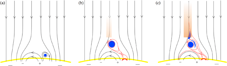
Images from the Hinode/X-ray telescope (XRT) show X-ray jets in coronal holes occurring at a rate $\sim$ 60/day, with average widths of 8000 km and lifetimes of $\sim$ 10 min (Savcheva et al., 2007). (See, e.g. Shimojo et al., 1996, for active-region-jet parameters.) Many, if not all, X-ray jets have EUV-jet counterparts (e.g. Raouafi et al., 2008; Moore et al., 2013; Sterling et al., 2015). Various studies also show that X-ray jets usually have a brightening off to one side of their base; we refer to that brightening as the “jet bright point” (JBP). Sterling et al. (2015) found that a jet minifilament erupts from the location where the JBP forms. They concluded that polar-coronal-hole coronal jets are scaled-down versions of typical-sized filament eruptions that drive a coronal mass ejection (CME) and produce a solar flare at the site of the pre-eruption filament, where analogously the minifilament eruption drives the jet and produces a miniflare (the JBP) at the site of the pre-eruption minifilament. Sterling et al. (2016) found that at least some active-region coronal jets also result from minifilament eruptions. Figure 1 shows their schematic interpretation of the mechanism producing the jets.

What leads to the minifilament eruptions has not yet been addressed systematically. Several on-disk studies of individual jets suggest that nearly-concurrent flux cancelation frequently occurs at the base (e.g., Huang et al., 2012). In the neighborhood of active regions, there is evidence that sometimes emerging flux together with canceling flux lead to the minifilament eruptions (Chandrashekhar et al., 2014; Sterling et al., 2016).

3 Spicules as Small-Scale Coronal Jets?

Just as CMEs and coronal jets respectively are consequences of filament eruptions and minifilament eruptions, perhaps spicules are consequences of even-smaller-scale microfilament eruptions.

To consider this suggestion’s plausibility, we estimate the size-scale distribution of erupting filament-like objects from the number of eruptions of three size classes: eruptions of typical filaments, minifilaments, and (if they exist) microfilaments, respectively corresponding to CME/flare eruptions, coronal jets, and spicules.

For typical-filament lengths, Bernasconi et al. (2005) gives a range of $3\times 10^{4}$ — $1.1\times 10^{5}$ km; we will use $(7\pm 4)\times 10^{4}$ km. For minifilaments, Sterling et al. (2015) found sizes of $(8\pm 3)\times 10^{3}$ km. Next we must estimate what size a postulated spicule microfilament might be. We note that the average measured size of 8000 km for the length of coronal-jet minifilaments from Sterling et al. (2015) is the same as the average width of X-ray jets measured by Savcheva et al. (2007). Similarly we hypothesize that the spicule-microfilament length would be about equal to the spicule width, which is $\sim$ 300 km (Pereira et al., 2012); we assume a range $\pm 100$ km.

How many of each class of filament eruption at a time might we expect? A value is readily available for the number of spicules (reaching above 3000 km) on the Sun at any time: that is $9.3\times 10^{4}$ from Athay (1959). Lynch et al. (1973) suggest numbers of $\raisebox{-4.30554pt}{$\stackrel{{\scriptstyle\textstyle<}}{{\sim}}$}5$ -times higher; we will use this as our upper limit. We do not know a similar quote for the number of coronal jets on the Sun at any given time, but we estimate this using the value of 60 X-ray jets/day in the two polar coronal holes from Savcheva et al. (2007). Averaged over a day, this is 2.5 jets/hour, or 0.42 jets every 10 min. Since the average lifetime of a jet is 10 min (Savcheva et al., 2007), we expect $\sim$ 0.5 jet among the two polar coronal holes at any given time (i.e., looking at two independent times will likely detect one jet on average). At the time of the Savcheva et al. (2007) study, each of the two polar coronal holes covered $\stackrel{{\scriptstyle\textstyle<}}{{\sim}}$ 5% of the Sun’s surface (Hess Webber et al., 2014). So we might guess that there would be about ten times the number of jets over the whole Sun as were in the polar coronal holes. (Coronal jets are common in active regions and quiet Sun, e.g., Shimojo et al. 1996, in addition to coronal holes.) So we estimate that there are $\sim$ 5 coronal jets on the Sun at any given time. For “typical” filament eruptions, we note that CMEs occur at between 0.5 and 6 per day (Yashiro et al., 2004; Chen, 2011); using a C/M-class flare’s strong-phase duration (NOAA-listed end-minus-start time) of $\sim$ 20 min (Veronig et al., 2002) to estimate a CME’s filament-eruption-phase duration gives $\sim$ 0.03 CME-producing typical filament eruptions occurring on the Sun at any given time.

Figure 2 plots these values, giving a number-versus-size distribution for filament-eruption-like events on the Sun, going down to microfilament eruptions postulated to produce spicules. This plot indicates that the idea of a microfilament-eruption origin of spicules is consistent with a power-law distribution of filament sizes from large-scale erupting filaments of typical solar eruptions, through erupting coronal-jet minifilaments and on down to spicule-producing erupting microfilaments.

If spicules are more numerous than the above-cited measurements determined, as perhaps indicated by Hinode/SOT observations, then our extrapolated distribution might substantially underestimate the number of spicules. In that case only a fraction of spicules may result from erupting microfilaments. In at least some cases however, the Hinode/SOT observations show many narrow spicule strands within a wider-erupting feature, giving an overcount of spicule-producing eruptions (Sterling et al., 2010a). Further studies should address this question.

4 Consequences and Expectations for Microfilament-Eruption Spicules

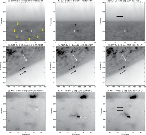
If microfilament eruptions drive spicules, we would expect a brightening corresponding to the JBP observed in solar jets (Fig. 1). Earlier numerical-simulation spicule models predicted brightening at the base of spicules near the time of their formation, but lack of identification of such brightenings in H $\alpha$ (Suematsu et al., 1995) has been presented as evidence against such models (Sterling, 2000). More recently however, subtle brightenings at the base of some rising spicules have been observed by Sterling et al. (2010b) in near-limb Hinode/SOT Ca ii movies. They found a plethora of small ( $\raisebox{-4.30554pt}{$\stackrel{{\scriptstyle\textstyle<}}{{\sim}}$}0^{\prime\prime}.5$ ), transient (few-100 s lifetime) “Ca ii brightenings” moving laterally at $\sim$ 10 km s^-1, some of which occurred when and where spicules formed. Figures 3(a—c) and 3(d—f) show two other such SOT Ca ii episodes, processed only with “fg_prep” and an unsharp mask. On-disk spicules are difficult to see in SOT/Ca ii images (Beck et al., 2013), and only a few are identifiable just inside the limb; some brightenings may be source locations for some invisible-against-the-disk spicules. In Figure 3(g—i) we show a Hinode/XRT X-ray jet from Sterling et al. (2015), with a color-reversed scaling. Except for the size-scale difference, coronal-jet morphology in the X-ray images is similar to the spicule morphology in the SOT images, in terms of the jet/spicule base brightenings. (Non-color-reversed XRT and AIA images and movies of the Figure 3(g—i) jet are available in Sterling et al. 2015.) Thus it is plausible that some base brightenings and accompanying spicules in the SOT Ca ii movies may be due to microfilament eruptions, just as the JBP brightenings and coronal jets in the XRT and AIA movies are due to minifilament eruptions. (See, e.g., Rutten & Uitenbroek 1991 and Sterling et al. 2010b for possible non-microfilament-eruption causes for Ca ii brightenings.)

Transient brightenings and small-scale jets are also seen at transition region temperatures by the Interface Region Imaging Spectrograph (IRIS) spacecraft (Tian et al., 2014), and base brightenings of small-scale active region Hinode/Ca ii-observed “Ca jets” (Shibata et al., 2007) are also candidates for base brightenings from putative microfilament eruptions.

There is evidence that coronal jets consist of two components: a hotter component, visible in X-rays and in hotter AIA EUV channels such as 171 Å, 193 Å, and 211 Å; and a cooler component frequently visible in cooler AIA EUV channels, especially 304 Å (Moore et al., 2013; Sterling et al., 2015). In the erupting-minifilament picture we expect the hotter component to form when the outer envelope of the exploding minifilament field (the part that does not contain minifilament material) undergoes reconnection with the ambient coronal field (“envelope reconnection”; Fig. 1(b)), and the cooler jet to form when the core of the exploding field (the part containing the cool material) undergoes that reconnection (“core reconnection”; Fig. 1(c)). Similar core and envelope reconnections should occur if microfilament eruptions make spicules. In that case, analogously, the core reconnection would expel upward cool chromospheric material to form the commonly-observed chromospheric spicules, while the envelope reconnection could produce the EUV spicules reported by De Pontieu et al. (2011) (and perhaps also UV spicules); the EUV spicules would be a co-produced hotter component of chromospheric spicules, and would not necessarily imply that spicules supply a large portion of the corona’s hot material (Madjarska et al., 2011; Klimchuk & Bradshaw, 2014). Additionally, the microfilaments might either fully erupt, or be partially confined, as with minifilaments (Sterling et al., 2015).

5 Summary and Discussion

Recent observations indicate that coronal jets result from minifilament eruptions, and so a natural suggestion is that spicules result from eruptions of even smaller “microfilaments” (cf. Moore, 1990). Moore et al. (2011) considered that spicules are small-scale jets, but that was based on earlier theoretical ideas of how coronal jets worked (e.g. Shibata et al., 1992), prior to our inferred minifilament scenario of Figure 1 (Sterling et al., 2015). Based on that new picture, our rough estimation of the number distribution of filament-eruption events (Fig. 2) allows that the majority of spicules could operate in this fashion.

A microfilament-eruption mechanism could address several hitherto-puzzling aspects of spicules:

•

Spicule energy source. Non-potential magnetic energy stored in the core of the pre-eruption microfilament field would power the spicules.
•

Smooth rise trajectories. Hinode observations indicate that spicules accelerate smoothly (e.g. De Pontieu et al., 2007), which is different from the predicted velocity jumps of some earlier models (see Sterling, 2000). Cool coronal jets (likely due to minifilament eruptions) observed in AIA 304 Å images also follow smooth trajectories (Moschou et al., 2013). So analogously we would expect microfilament eruptions to result in spicules following smooth trajectories, as observed (although detailed comparisons of the respective trajectories have not yet been made).
•

Twisting spicules. Long-suspected twisting of spicules have now been observed with confidence (e.g. De Pontieu et al., 2012). Twisting is also observed in coronal jets, including ones clearly due to minifilament eruptions (Moore et al., 2015, and references therein). This twist could be conveyed from the erupting closed, twisted field carrying the minifilament to open ambient field by the external reconnection of Figure 1(b), and 1(c), as in Shibata & Uchida (1986). A similar process could explain twisting of spicules if they result from microfilament eruptions.
•

Spicule lateral motions. De Pontieu et al. (2012) and other workers note transverse motions of spicules. Lateral (transverse) motions also occur on X-ray jets (Cirtain et al., 2007; Savcheva et al., 2007). A jet from an erupting micro- or minifilament might acquire undulatory horizontal motion from the reconnection with the ambient field; cf. Fig. 1(b). Also, this reconnection could produce progressive illumination of the ambient field lines, resulting in apparent splitting (Sterling et al., 2010b).
•

Hotter spicule components. EUV and UV spicules (§4 above, and references in Sterling 2000) could result naturally when the envelope of the microfilament field carrying less-dense material reconnects with the ambient field (§4).
•

Gap at spicule bases. The sometimes-observed gap between the photospheric limb and the bottoms of spicules (e.g., Gaizauskas, 1984) could result from the spire of the spicule forming by reconnection at the height of the neighboring bipole (Fig. 1).

We can estimate the pre-eruption magnetic field strength, $B$ , required for the postulated microfilament flux ropes (cf. Falconer et al., 2003) that erupt to produce spicules. Sterling (2000) estimates a spicule to have energy $\stackrel{{\scriptstyle\textstyle<}}{{\sim}}$ 10²⁵ erg. (Dimensions for a type II spicule from, e.g., Pereira et al. 2012, are smaller than those assumed in Sterling 2000, implying lower energy. But their type II spicule speeds are larger than assumed in Sterling 2000, and Alfvén wave energy was not included in Sterling 2000 and could add $\sim$ 50% to the energy (Moore et al. 2011). So $\sim$ 10²⁵ erg is a reasonable estimate.) We equate this to the flux-rope total magnetic energy of $V(B^{2}/8\pi)$ , where the flux rope of length $l$ and radius $r$ has volume $V$ of $\pi r^{2}l$ . Taking $l\sim$ 500 km (about the size of the Ca ii brightenings in Fig. 3, and similar to spicule width used in Sterling 2000), and estimating $l/r\sim 10$ (as in filaments; cf. Falconer et al., 2003), gives $B\sim 250$ G for the flux rope, and hence for the host bipole. Network-boundary magnetic cancelations of this size are observed (e.g. Gos̆ić et al., 2016), but it has not yet been demonstrated that the strength of the canceling field is of the correct magnitude or that the canceling field is connected to spicules.

We can estimate the temperature regime in which the base brightenings should appear by equating the estimated spicule energy, $E,$ deposited in a volume, $V,$ as thermal energy, $(3/2)nVkT$ , where $n$ , $k$ , and $T$ are particle number density, Boltzmann’s constant, and temperature, respectively. With $V$ as above, this gives $E\sim[(3/2)10^{-2}\pi k]nl^{3}T.$ For a spicule/microfilament, using $E$ and $l$ as above, and $n\sim 10^{14}$ cm^-3 (Vernazza et al., 1981, model C at 755 km), gives $T\sim 10^{5}$ K, consistent with chromospheric/transition region emission (e.g., H $\alpha$ , Si iv). For a jet/minifilament, taking $E\sim 10^{27}$ erg (Pucci et al., 2013), $l=8000$ km (Sterling et al., 2015), and $n\sim 10^{11}$ (Vernazza et al., 1981, model C at 1990 km), gives $T\raisebox{-4.30554pt}{$\stackrel{{\scriptstyle\textstyle>}}{{\sim}}$}10^{6}$ K, consistent with coronal emission. Modeling is required to test in detail predictions of the proposed mechanism.

Theoretical calculations suggest that type I spicules might result from p-mode oscillations (e.g., Hansteen et al., 2006). Erupting microfilaments also might occur in active regions too, leading to type I spicules. Moreover, p-mode oscillations could conceivably drive repeated cancelations, each leading to an erupting microfilament flux rope (perhaps driving waves/shocks). This is still speculation, however.

Our conjectured microfilaments may have not yet been detected because of their expected small size ( $\stackrel{{\scriptstyle\textstyle<}}{{\sim}}$ 0. ${}^{\prime\prime}5$ — $1^{\prime\prime}.0$ ). In addition, Sterling et al. (2016) suggested that minifilaments that cause jets in active regions might often not be visible when low to the photosphere because of surrounding obscuring material. Similarly, spicule-producing microfilaments might be unobscured, and hence observable, only infrequently. Finally, the microfilament-carrying twisted-core magnetic bipole might only be created near or during the microfilament-eruption time, making the pre-eruption microfilament short lived. Further observations may provide additional hints as to whether microfilament eruptions make spicules, but a clear determination may have to await a new generation of instruments, such as DKIST or the next space-based follow on to Hinode/SOT.

This work was supported by funding from the Heliophysics Division of NASA’s Science Mission Directorate through the Heliophysics Guest Investigator (HGI) Program, and the Hinode Project. We thank T. Tarbell for assistance with SOT images. Hinode is a Japanese mission developed and launched by ISAS/JAXA, with NAOJ as domestic partner and NASA and STFC (UK) as international partners, and operated by these agencies in co-operation with ESA and NSC (Norway). Figure 1, and Figure and video 3(g—i), adapted by permission from Macmillan Publishers Ltd: Nature, Sterling et al. (2015), copyright 2015.

References

Athay (1959) Athay, R. G. 1959, ApJ, 129, 164
Beck et al. (2013) Beck, C., Rezaei, R., & Puschmann, K. G. 2013, A&A, 556, 127
Beckers (1968) Beckers, J. M. 1968, Sol. Phys., 3, 367
Bernasconi et al. (2005) Bernasconi, P. N., Rust, D. M., & Hakim, D. 2005, Sol. Phys., 228, 97
Chandrashekhar et al. (2014) Chandrashekhar, K., Morton, R. J., Banergee, D., & Gupta, G. R. 2014, A&A, 562, 98
Chen (2011) Chen, P. F. 2011, LRSP, 8, 1
Cirtain et al. (2007) Cirtain, J. W., Golub, L., Winebarger, A. R., et al. 2007, Science, 318, 1580
De Pontieu et al. (2004) De Pontieu, B., Erd’elyi, R., & James, S. P. 2004, Nature, 430, 536
De Pontieu et al. (2007) De Pontieu, B., McIntosh, S., Hansteen, V. H., et al. 2007, PASJ, 59, S655
De Pontieu et al. (2011) De Pontieu, B., McIntosh, S. W., Carlsson, M., et al. 2011, Science, 331, 55
De Pontieu et al. (2012) De Pontieu, B., Carlsson, M., Rouppe van der Voort, L. H. M., et al. 2012, ApJ, 752L, 12
Falconer et al. (2003) Falconer, D. A., Moore, R. L., Porter, J. G., & Hathaway, D. H. 2003, ApJ, 593, 549
Gaizauskas (1984) Gaizauskas, V. 1984, Sol. Phys., 93, 257
Gos̆ić et al. (2016) Gos̆ić, M., Bellot Rubio, L. R., del Toror Iniesta, J. C., Orozco Suárez, D., & Katsukawa, Y. 2016, ApJ, 820, 35
Hansteen et al. (2006) Hansteen, V. H., De Pointieu, B., Rouppe van der Voort, L., van Noort, M., & Carlsson, M. 2006, ApJ, 647L, 73
Hess Webber et al. (2014) Hess Webber, S. A., Karna, N., Pesnell, W. D., & Kirk, M. S. 2014, Sol. Phys., 289, 4047
Huang et al. (2012) Huang, Z., Madjarska, M. S., Doyle, J. G., & Lamb, D. A. 2012, A&A, 548, A62
Iijima & Yokoyama (2015) Iijima, H. & Yokoyama, T. 2015, ApJ, 812L, 30
Klimchuk & Bradshaw (2014) Klimchuk, J. A., & Bradshaw, S. J. 2014, ApJ, 791, 60
Lynch et al. (1973) Lynch, D. K., Beckers, J. M., & Dunn, R. B. 1973, Sol. Phys., 30, 63L
Madjarska et al. (2011) Madjarska, M. S., Vanninathan, K., Doyle, J. G. 2011, A&A, 532L, 1
Martinez-Sykora et al. (2013) Martinez-Sykora, J., De Pontieu, B., Leenaarts, J., et al. 2013, ApJ, 771, 66
Moore (1990) Moore, R. L. 1990, Mem. Soc. Astron. Ital., 61, 317
Moore et al. (2011) Moore, R. L., Sterling, A. C., Cirtain, J. W., & Falconer, D. A. 2011, ApJ, 731L, 18
Moore et al. (2013) Moore R. L., Sterling A. C., Falconer D. A. & Robe D. 2013 ApJ, 769 134
Moore et al. (2015) Moore, R. L., Sterling, A. C., & Falconer, D. A. 2015, ApJ, 806, 11
Moschou et al. (2013) Moschou, S. P., Tsinganos, K., Vourlidas, A., & Archontis, V. 2013, Sol. Phys., 284, 427
Nisticò (2009) Nisticò, G., Bothmer, V., Patsourakos, S., & Zimbardo, G. 2009, Sol. Phys., 259, 87
Pereira et al. (2012) Pereira, T. M. D., De Pontieu, B., & Carlsson, M. 2012, ApJ, 759, 18
Pereira et al. (2013) Pereira, T. M. D., De Pontieu, B., & Carlsson, M. 2013, ApJ, 764, 69
Pucci et al. (2013) Pucci, S., Poletto, G., Sterling, A. C., & Romoli, M. 2013, ApJ, 776, 16
Raouafi et al. (2008) Raouafi, N.-E., Petrie, G. J. D., Norton, A. A., Henney, C. J., & Solanki, S. K. 2008, ApJ, 682, L137
Rutten & Uitenbroek (1991) Rutten, R. J. & Uitenbroek, H. 1991, Sol. Phys., 134, 15
Savcheva et al. (2007) Savcheva, A., Cirtain, J. W., DeLuca, E. E., et al. 2007, PASJ, 59S, 771S
Shibata & Uchida (1986) Shibata, K., & Uchida, Y. 1986, Sol. Phys., 103, 299
Shibata et al. (1992) Shibata, K., Ishido, Y., Acton, L. W., et al. 1992, PASJ, 44, 173L
Shibata et al. (2007) Shibata, K., Nakamura, T., Matsumoto, T., et al. 2007, Science, 318, 1591
Shimojo et al. (1996) Shimojo, M., Hashimoto, S., Shibata, K., Hirayama, T., Hudson, H. S., & Acton, L. W. 1996, PASJ, 48, 123
Skogsrud et al. (2015) Skogsrud, H., Rouppe van der Voort, L., De Pontieu, B., & Pereira, T. M. D. 2015, ApJ, 806L, 170
Sterling (2000) Sterling, A. C. 2000 Sol. Phys., 196, 79
Sterling et al. (2010a) Sterling, A. C., Harra, L. K., & Moore, R. L. 2010a, ApJ, 722, 1644
Sterling et al. (2010b) Sterling, A. C., Moore, R. L., & DeForest, C. E. 2010b, ApJ, 714L, 1
Sterling et al. (2015) Sterling, A. C., Moore, R. L., Falconer, D. A., & Adams, M. 2015, Nature, 523, 437
Sterling et al. (2016) Sterling, A. C., Moore, R. L., Falconer, D. A., et al. 2016, ApJ, 821, 100
Suematsu et al. (1995) Suematsu, Y., Wang, H., & Zirin, H. 1995, ApJ, 450, 411
Tian et al. (2014) Tian, H., DeLuca, E. E., Crammer, S. R., et al. 2014, Science, 346, 315
Vernazza et al. (1981) Vernazza, J. E., Avrett, E. H., & Loeser, R. 1981, ApJS, 45, 635
Veronig et al. (2002) Veronig, A., Temmer, M., Hanslmeier, A., Otruba, W., & Messerotti, M. 2002, A&A, 382, 1070
Yashiro et al. (2004) Yashiro, S., Gopalswamy, N., Michalek, G., et al. 2004, JGRA, 109, 7105
Zhang et al. (2012) Zhang, Y. Z., Shibata, K., Wang, J. X., et al., ApJ, 750, 16

Refer to caption — Figure 1: Schematic of minifilament eruption leading to a coronal jet (modified version of Sterling et al. 2015, Fig. 2). Black lines show magnetic fields, with arrows indicating polarities. Red lines indicate fields that have undergone magnetic reconnection, with red “X”-es showing reconnection locations. (a) Initially, a minifilament (blue) sits in a compact sheared bipole adjacent to a larger less-sheared bipole, all inside surrounding open field. (b) An unspecified agent triggers the minifilament field to erupt like a larger-scale filament eruption. Reconnection at the left-side red X between the envelope of the erupting minifilament field and the open coronal field results in a hot jet (shaded-orange strip), visible as a hotter-EUV (e.g., 211 Å) or X-ray jet. Reconnection interior to the exploding minifilament field at the right-side red X results in the JBP (bold red semicircle), analogous to a solar flare in large-scale filament eruptions. (c) If the minifilament erupts far enough into the opposite-polarity open-field region, then the left-side reconnection “eats away” enough of the enveloping outer field surrounding the minifilament in the core for minifilament material to be expelled along the vertical field, resulting in a cool (e.g., EUV 304 Å) jet component. See Sterling et al. (2015, 2016) for details.