Playing Doom with SLAM-Augmented Deep Reinforcement Learning
Abstract
A number of recent approaches to policy learning in 2D game domains have been successful going directly from raw input images to actions. However when employed in complex 3D environments, they typically suffer from challenges related to partial observability, combinatorial exploration spaces, path planning, and a scarcity of rewarding scenarios. Inspired from prior work in human cognition that indicates how humans employ a variety of semantic concepts and abstractions (object categories, localisation, etc.) to reason about the world, we build an agent-model that incorporates such abstractions into its policy-learning framework. We augment the raw image input to a Deep Q-Learning Network (DQN), by adding details of objects and structural elements encountered, along with the agent’s localisation. The different components are automatically extracted and composed into a topological representation using on-the-fly object detection and 3D-scene reconstruction. We evaluate the efficacy of our approach in “Doom”, a 3D first-person combat game that exhibits a number of challenges discussed, and show that our augmented framework consistently learns better, more effective policies.
1 Introduction
Recent approaches to policy learning in games [30, 29] have shown great promise and success over a number of different scenarios. A particular feature of such approaches is the ability to take the visual game state directly as input and learn a mapping to actions such that the agent effectively explores the world and solves predetermined tasks. Their success has largely been made possible thanks to the ability of deep reinforcement learning (deepRL) networks, neural networks acting as function approximators within the reinforcement-learning framework. A particular variant, Deep Q-Learning Networks (DQN), has been widely used in a range of different settings with excellent results. It employs convolutional neural networks (CNN) as a building block to effectively extract features from the observed input images, subsequently learning policies using these features.
For the majority of scenarios that have been tackled thus far, a common characteristic has been that the domain is 2-dimensional. Here, going directly from input image pixels to learned policy works well due to two important factors: i) a reasonable amount of the game’s state is directly observable in the image, and ii) a combination of a lower-dimensional action space and smaller exploration requirements result in a smaller search space. The former ensures that the feature extraction always has sufficient information to influence policy learning, and the latter makes learning consistent features easier. Despite stellar success in the 2D domain, these models struggle in more complicated domains such as 3D games.
 |
 |
 |
 |
 |
 |
3D domains exhibit a multitude of challenges that cause the standard approaches discussed above to struggle. The introduction of an additional spatial dimension, first introduces notions of partial observability and occlusions, and secondly causes complications due to viewpoint variance. Not only is the agent viewing a relatively smaller portion (volume) of the environment, it also must reconcile observing a variety of other objects in different contexts under projective transformations. Furthermore, adding an extra dimension also combinatorially complicates matters in terms of exploration of the environment. This typically manifests itself in the form of sparse feedback in the learning process because the agent’s inability to explore the environment directly penalizes its learning capacity. Moreover, complications in exploration directly affect any planning that may be required for tasks and actions. Finally, with larger search and state spaces comes the likelihood that any rewards that might help move learning along are also harder to come by.
Sutton et al. (1999) [42] propose an extension of the RL framework that can potentially learn hierarchical policies. However this, and similar methods, have not been able to scale beyond small gridworld domains [1]. Kulkarni et al. (2016) [24] proposes to tackle environments with delayed rewards by coupling options learning and intrinsically driven exploration methods. Options are however notoriously hard to train, requiring a great deal of effort before intrinsically motivated agents can safely deal with generic hierarchical spatial domains.
Prior work in behavioural modelling and cognitive neuroscience suggests that humans employ particular, highly specialised mechanisms to construct representations of, and reason about, the world. These typically take the form of semantic concepts and abstractions such as object identity, categories, and localisation. Freedman and Miller (2008) [14] review evidence from neurophysiology that explore the learning and representation of object categories. Burgess (2008) [4] discusses evidence from neuroscience for the presence and combination of different viewpoints (e.g., egocentric) and the role of representing layouts (e.g., boundaries and landmarks) in the spatial cognition process. Moser et al. (2008) [31] also discuss the presence of highly specialised representation regions in the brain that encode localisation and spatial reasoning. Denis and Loomis (2007) [7] provide a review from behavioural psychology on the subject of spatial cognition and related topics.
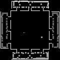
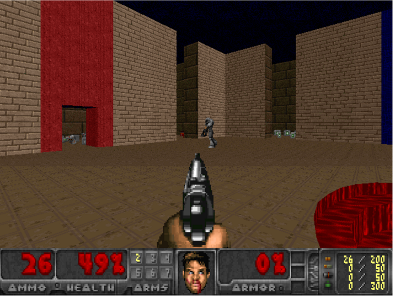
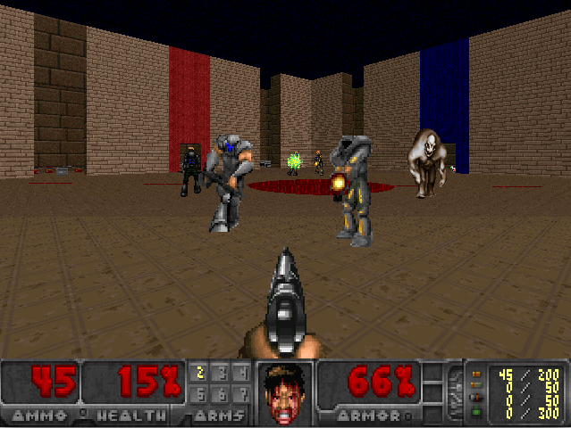
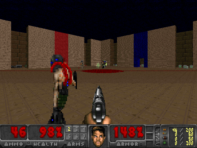
In this paper, we take inspiration from such work to propose a system that explicitly constructs a joint semantic and topological representation of the state, and further augment its input with this representation (Fig. 1) in an attempt to learn policies more effectively in such complex 3D domains. To this end, we construct a novel model that incorporates an automatic, on-the-fly scene reconstruction component into a standard deep-reinforcement learning framework. Our work provides a streamlined system to immediately enhance current state-of-the-art learning algorithms in 3D spatial domains, additionally obtaining insight on the efficacy of spatially enhanced representations against those learned in a purely bottom-up manner.
2 Related work
2.1 Deep Reinforcement Learning
Reinforcement Learning is a commonly employed set of techniques for learning agents that can execute generic and interactive decision making. Its mathematical framework is based on Markov Decision Processes (MDPs). An MPD is a tuple , where is the set of states, is the set of actions the agent can take at each time step , is the transition probability of going from state to using action , is the reward function defining the signal the agent receives after taking actions and changing states, and is a discount factor. The goal of Reinforcement Learning is to learn a policy that maximises the expected discounted average reward over the agent run. A commonly used technique to learn such a policy is to learn the action-value function iteratively, so as to gradually approximate the expected reward in a model-free fashion.
They have, however, traditionally struggled to deal with high-dimensional environments, due in large part to the curse of dimensionality. Deep Reinforcement Learning algorithms such as Deep-Q Networks extend model-free RL algorithms like Q-Learning to use Deep Neural Networks as function approximators, implicitly capturing hierarchies in the state representation that make the RL problem scale even to visual input states. Unfortunately, they still suffer from some of the problems that standard RL cannot deal with:
-
•
delayed reward signals require non-stochastic exploration strategies [24];
-
•
learning to abstract policies hierarchically is currently an unsolved but key problem to make RL scale to tasks requiring long-term planning [1];
-
•
partial observability in state requires use of models that can encode at least short-term memory, specially when training end-to-end [17].
Some recent work has also explored ways to develop agents that can learn to play Doom. Lample and Chaplot (2016) [25] take the approach of using a variant of DRQN [18] together with some game features extracted directly from the game environment through its data structures. Our method is similar in the spirit, but can be applied to any environment with a significant 3D navigation component, as our SLAM and object recognition pipeline is not intrinsically dependent to the VizDoom platform. Another interesting approach is the one presented by Dosovitskiy and Koltun (2016) [8]. This approach, featured as the winner in the VizDoom competition [20], changed the supervision signal from a single scalar reward to a vector of measurements provided by the game engine. This is used to train a network that, given the visual input, the current measurements, and the goal, predicts future measurements. The action to perform is then chosen greedily according the predicted future measurements. This is orthogonal to our approach; both algorithms could benefit from the novelties introduced by the other, however we leave such an extension on our part for the future.
2.2 Simultaneous Localization and Mapping
Early approaches to camera-pose estimation relied on matching a limited number of sparse feature points between consecutive video frames [6]. A common drawback of such solutions is relatively quick error accumulation which results in significant camera drift. This may be addressed with PTAM [22], which achieved globally optimal solutions at real-time rates by running bundle adjustment in a background thread. Further improvements include re-localization, loop-closure detection, and faster matching with binary features [5, 32, 23]. Recently, matching hand-crafted features has been replaced by semi-dense direct methods [10]. However, these approaches only provide very limited information about the environment.
A more complete map representation is provided by dense approaches [41, 34, 27]. They estimate dense depth from monocular camera input, but their use of a regular voxel grid limits reconstruction to small volumes due to memory requirements. KinectFusion-based approaches [33] sense depth measurements directly using active sensors and fuse them over time to recover high-quality surfaces, but they too suffer from the same issue. This drawback has since been removed by scalable approaches that allocate space only for those voxels that fall within a small distance of the perceived surfaces, to avoid storing unnecessary data for free space [35]. All approaches mentioned above assume the observed scenes are static. This assumption can be relaxed by full SLAM with generalized (moving) objects or some of its more efficient variants [45, 3], but this is beyond the scope of this paper.
Approaches such as RatSLAM [28] and its derivatives propose instances of SLAM based on models inspired by biological agents, showing promising results in environments where the navigation task requires some reasoning about landmarks and non-Cartesian grid representations.
2.3 Object detection
Early approaches to object detection include constellation models and pictorial structures [13]. The very first object detector capable of real-time detection rates was [44], who solved an inherent problem of sliding-window approaches by learning a sequential decision process that rapidly rejects locations which are unlikely to contain any objects. This concept has since then evolved into a distinct set of algorithms called proposals, whose only goal is to quickly localize potential objects [19]. These locations are then fed into more complex classifiers to determine the class label (or assign a background). Deformable part models [11] are a prominent example of such, being able to represent highly variable object classes. Recently, it has been shown that deformable part models can be interpreted as a convolutional network [16], which led to replacement of handcrafted features by convolutional feature maps [15]. Finally the Faster-RCNN [36] combines the region proposals and object detector into a single unified network trainable end-to-end with shared convolutional features which leads to very fast detection rates.
3 Semantic Mapping
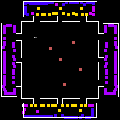
In this paper, we introduce an algorithm based on the Deep Q Network (DQN) that has been successfully applied to many Atari games [30]. Inspired by prior work in human cognition that indicates how humans employ a variety of semantic concepts and abstractions (object categories, localization, etc.) to reason about the world, we build an agent-model that incorporates such abstractions into its policy-learning framework. We augment the first-person raw image input to a DQN by adding details about objects and structural elements encountered, along with the agent’s localization to cope with complex 3D environments. This is represented as a 2D map (top-down view) encoding three distinct sources of information: i) positions of static structures and obstacles such as walls, ii) position and orientation of the agent, and iii) positions and class labels of important objects such as health packs, weapons and enemies. Our representation is being updated over time as the agent explores the environment. This allows the agent to keep information about areas observed in the past and build an aggregated model of the 3D environment, as indicated in Fig. 1. Such representation allows the agent to behave properly even with respect to the elements no longer present in the first-person view.
Semantic representation.
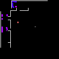
As the agent explores the environment, we simultaneously estimate localization of the agent and obstacles (e.g., walls) in order to build the map of the surrounding 3D environment from the first-person-view at each frame. In parallel, we detect important objects in the scene such as weapons and ammunition. And since we want to minimize the dimensionality of the augmented representation to allow more efficient learning, we project all semantic information onto a single common 2D map of a fixed size. Essentially a “floor-plan” with the positions of objects and agents. This is achieved by encoding different entities by different gray-scale values, in the form of heat-maps (cf., bottom right of Fig. 1).
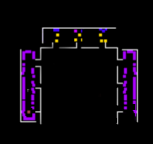
Our representation encodes position of walls and obstacles (white) extracted directly from the depth data provided by the VizDoom API. Information about agent’s position and orientation on the 2D map is represented as a green directed arrow. We also want to provide the agent semantic information about a variety of objects present in the environment. For Doom, we encode the following five object categories: monsters (red), health packs (purple), high-grade weapons (violet), high-grade ammunition (blue), other weapons and other ammunition (yellow). Since these objects could either move or be picked up by another player (e.g., deathmatch scenario), we project only those objects that are visible in the current view onto the common map. This could be addressed by more advanced data association techniques such as [45, 3], but this is beyond the scope of this paper.
4 Recognition and Reconstruction
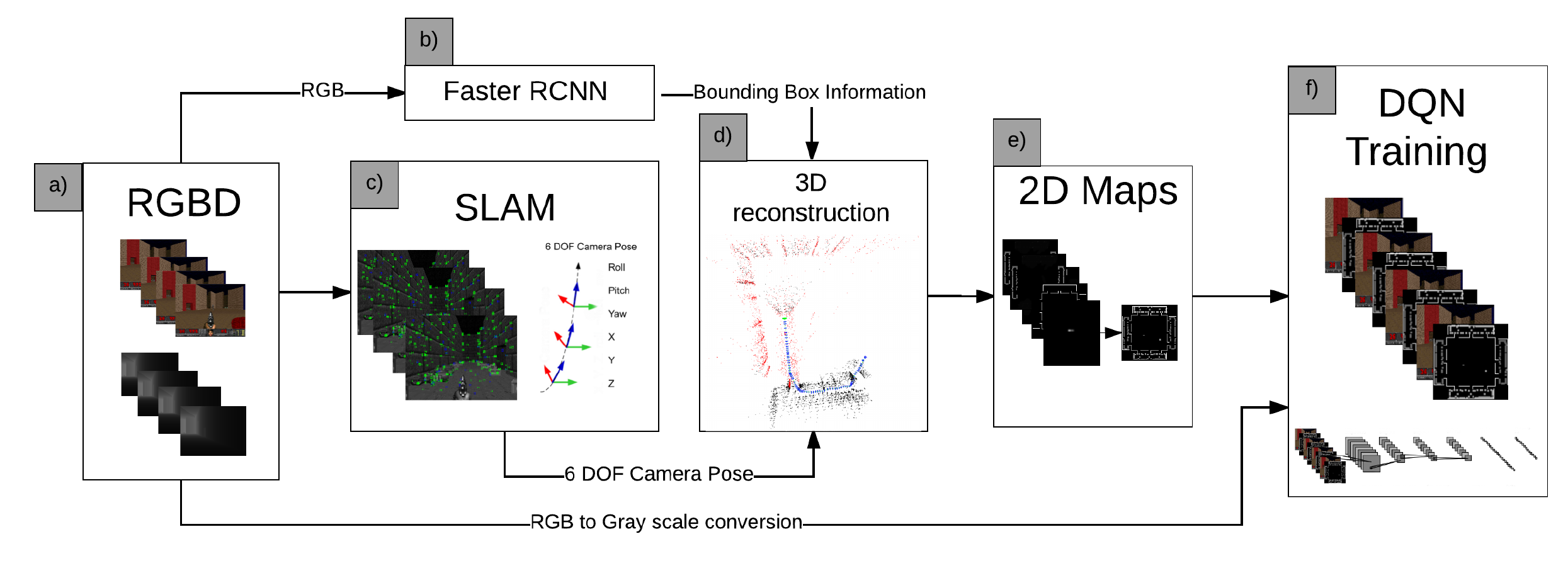
Here, we describe the process of automatically creating semantic maps on-the-fly. Fig. 2 depicts the architecture of our pipeline. As input, we use the image data provided by the VizDoom API, i.e., RGB video frames visualizing the 3D environment from agents (first person) perspective and a z-buffer providing depth information of the observed scene. In order to build a map of the 3D environment, we need to detect and remove all objects from the z-buffer since we want to i) provide explicit semantic information about various objects (monsters, weapons, etc.) and ii) avoid nuisance visual events such as weapon discharges in the depth buffer. We also need to know the current pose of the camera, so we run a camera-pose tracker in parallel with the object detector. Then, we project the observed scene on a common 3D map and provide its 2D visualization (top-down view) to the agent. Note, that the mapping system could work even without access to the z-buffer, i.e., using solely the RGB data [9]. We now describe the components of our pipeline (object detection, camera pose estimation and map fusion) in greater detail.
4.1 Object detection
To detect the objects, we use the Faster-RCNN object detector [36], which is a convolutional network that combines the attention mechanism (region proposals) and object detector into a single unified network, trainable end-to-end. The first module is a deep fully-convolutional network that simultaneously predicts object bounds and objectness scores at each position, and the second module is the Fast R-CNN detector [15] that uses the proposed regions. Since both modules share the same features, it offers very fast detection rates.
As input, we use the RGB image resized to the standard resolution of pixels. Next, the image is pushed through the network and a convolutional feature map is extracted. We use the model of Zeiler and Fergus (2014) [47] to extract these feature maps. To generate region proposals, this feature map is processed in a sliding-window manner with two fully-connected layers predicting position of the region proposal and a binary class label indicating “objectness”. For each region proposal, the corresponding (shared) feature maps are fed into 2 fully-connected layers with 2048 units that produce soft-max probabilities over object classes (and background) and positions of bounding boxes of the detected objects. We trained this object detector on five classes corresponding to objects and monsters that are projected onto the common map.
4.2 Camera pose estimation
Despite using ground-truth depth maps provided by the z-buffer, ICP-like approaches [2] do not work well in game environments since such environments lack many geometrical features (they are typically represented as textured planar surfaces to allow fast rendering). Hence, we use the sparse feature-based ORB-SLAM2 for 6-DoF camera-pose estimation [32]. As input, we use RGB images down-sampled to pixels and a z-buffer.
First, we build an eight-level image pyramid with a scale factor . Then, we extract a set of sparse local features representing corner-like structures. For this, we use oriented multi-scale FAST detector [37] with an adaptively-chosen threshold to detect a sufficient number of features. The feature extraction step is biased by bucketing to ensure features are uniformly distributed across space and scale (at least 5 corners per cell). A constant-velocity motion model predicting the camera pose is used to constrain matching onto local search windows. The extracted features are associated with local binary-patterns (256 bits ORB [38]) and matched using a mutual-consistency check. A robust estimate is performed by RANSAC [12] with least-squares refinement on the inliers.
Robustness is further increased by keyframes that reduce drift when the camera viewpoint does not change significantly. If tracking is lost, the current frame is converted into a bag-of-words and queried against the database of keyframe candidates for global re-localization. The camera is re-localized using the PnP algorithm [26] with RANSAC. Global consistency is achieved by loop-closing pose-graph optimization that distributes the loop-closing error along the graph in a background thread [23].
4.3 Mapping
Once we have the camera poses and a object-masked depth map, we can project the current frame on a common 3D map. At each frame , we back-project all image pixels into the current camera reference frame to obtain a vertex map
| (1) |
Here, denotes the inverse of the camera calibration matrix (using parameters from the VizDoom configuration file), denote image pixels in homogeneous coordinates, and is depth. We also want to maintain previously-visited areas in memory so we project the (homogenized) vertex map from camera to global reference frame as , where is a rigid body transformation mapping the camera coordinate frame at time into the global frame . Since the fixed volumetric 3D representation severely limits the reconstruction size that can be handled, we use the hash-based method of [35].
The resulting 2D map is generated by placing a virtual camera at the top-down view, ignoring all points above and below some height thresholds to remove areas that would otherwise occlude the map, such as ceilings and floors.
5 Experiments
In this section, we demonstrate the advantage of adding the semantic map presented in Sec. 3 to the standard first-person view while working inside the “Doom” environment. Code and results for these experiments will be made available online. We use the ViZDoom [21] platform for all our experiments. It is built on top of the first person combat game “Doom”, and allows easy synchronous control of the original game, where execution is user-controlled, getting the first-person-view from the engine at the current step, and stepping forward by sending it keystrokes. The environment where the player performs is specified as scenario.
In this paper, we focus on the deathmatch scenario, in which the map is a simple arena as can be seen in Fig. 1 and the goal is to eliminate as many opponents as possible before being eliminated. A proficient agent for this scenario would be the one that is efficient at eliminating enemies whilst being able to both collect more effective weapons and keep its own health as high as possible. This scenario was the basis of the CIG 2016 competition [20] where different autonomous agent competed in a deathmatch tournament.
The quantitative results for all the experiments carried out are summarised in Tab. 1. The individual features of the experiments run, and the insights obtained from these runs, are described in subsequent sections, following detailed discussion of the various components of our framework.
| Settings | Rewards |
|---|---|
| Random Play | |
| NOSM (player/objects) | |
| OSM (no FPV) | |
| baseline | |
| NOSM (objects) | |
| NOSM (walls) | |
| Prior Dueling DQN | |
| RSM (localisation) | |
| OSM (localisation) | |
| RSM | |
| OSM | |
| Human Player |
Recognition and Reconstruction.
As described in Sec. 4.1, we use the Faster-RCNN detector and feed it with the RGB image given by the platform. We use a network pre-trained on Imagenet [39] that we fine-tuned on a dataset consisting of 2000 training and 1000 validation examples extracted from the ViZDoom engine, performing 5-fold cross-validation. These images were manually annotated with ground-truth bounding boxes corresponding to 7 classes: monsters, health packs, high-grade weapons, high-grade ammunition, other weapons/ammunition, monsters’ ammunition, and agent’s ammunition. After fine-tuning, the model achieved an average precision of . The reconstruction system presented in Sec. 4.2 uses the RGB-D images provided by the VizDoom platform.
Policy Learning.
We use the DQN framework from [30] to perform policy learning with our augmented features. The only modification to the original algorithm is the CNN architecture that needs to be able to cope with the extended state. The first person view (FPV) images are resized to pixel, converted to grayscale and normalized. The semantic 2D map is represented as a single channel image of the same resolution. The different object categories are encoded by different grayscale values. For the experiments that use both the FPV and the 2D map, we concatenate them along the channel dimension. The Q network is composed of 3 convolutional layers having respectively, 32, 64 and 64 output channels with filters of sizes , and and 4, 2 and 1 strides. The fully-connected layer has 512 units and is followed by an output SoftMax layer. All hidden layers are followed by rectified linear units (ReLU). Adding the 2D map associated to each FPV image changes input channels from 4 to 8 for the first convolutional layer, and thus increase the number of parameters from to , a increase. For training, we use the hyper-parameters from [29] and RMSProp for all experiments.
Action Space.
The action space for this environment is an order of magnitude larger than the Atari environment. Indeed, “Doom” accepts any combination of unique keystrokes as input. Following the observation that a human player uses only a small subset of these combinations to play the game, we recorded actions performed by humans and selected a representative subset. These actions can be divided into three groups: i) actions corresponding to a single keystroke allowing the agent to move and shoot, ii) combinations of two keystrokes corresponding to moving and shooting at the same time and iii) actions associated with switching weapons. We arbitrarily chose the top 13 actions performed by humans, categorising them into the 3 groups mentioned above. We did so primarily to constrain the action space to a reasonably tractable size, while still maintaining richness of actions that could be performed in the environment.
Reward Function.
Our reward function is designed to capture the primary goal of the agent: to eliminate opponents. We represent this as , an indicator variable for an opponent being eliminated since the last step. To encourage the agent to live longer, we also consider , the health variation between the current step and the previous step. We explicitly structure the health reward to be zero-sum in order to remove any biases towards preserving health to the detriment of the primary goal. The reward incorporating both these terms is written as: where and
Evaluation Metrics.
We use two different scores to evaluate and compare different architectures. The main metric is the reward function as it allows observing the agent’s behaviour with respect to the primary objective. The second reported metric is the number of steps the agent has lived. This is important as living increases the agent’s chance to kill opponents and increase its reward in the longer term. All reported metrics are mean values over test games.
Time Complexity.
The complete framework has to be fast enough to allow playing at the game’s native speed. To do so, we run the object detector in parallel with the camera-pose estimation. On average, the detector requires ms to process an image while camera-pose estimation and latency take ms and ms respectively. Semantic map construction takes ms, and DQN training requires ms to process a frame and perform one learning step. The complete pipeline is able to process, on average, 10 images per second. Given that inside the ViZDoom platform each step represents 4 frames of the game (as does the Atari emulator), our system plays at approximately 40 frames per second, which exceeds typical demands of gameplay. All experiments were run on a Intel Core i7-5930K machine with 32GB RAM and one NVidia Titan X GPU.
 |
 |
5.1 Oracle Semantic Maps (OSM)
The first set of experiments allows us to evaluate the efficacy of our semantic representation. We first isolate potential errors introduced by the recognition and reconstruction pipeline by extracting ground-truth information about classes and positions of all objects that are used in the semantic map representation. In other words, this experiment presents the results we would get if we had perfect detection and reconstruction, and is used as an “oracle”.
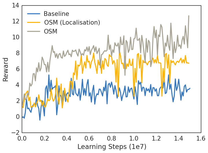
As the baseline, we use the standard DQN approach trained solely on the first person view images (referred to as baseline in the following). This baseline is compared to i) model trained with both, the first person view and the 2D map encoding ground-truth walls and player position (localisation OSM) ii) model trained with both, the first person view augmented by the complete 2D maps containing ground-truth walls and positions of player and objects.
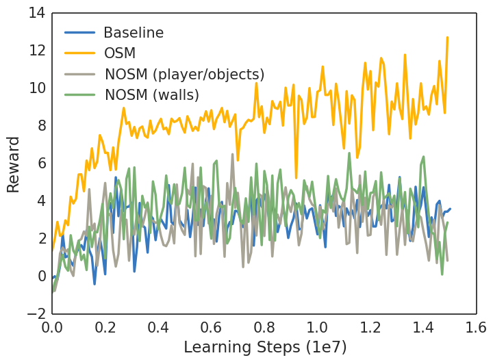
As can be seen in Fig. 3, the baseline is not able to learn as good policy as model with our semantic maps. Moreover, we see that the baseline model quickly reaches a plateau and does not improve afterwards. Adding a 2D map of the environment (i.e., without objects) allows the agent to learn a significantly better policy as the reward is almost doubled compared to the baseline. Adding the objects seen by the agent onto this map gives another significant improvement leading to reward of compared to the achieved by the baseline. Moreover, we can see that the network provided with the complete 2D map (including objects) is able to learn faster than the models provided with fewer information. This result proves that providing higher level, complex representation of the surrounding of the agent allows it to learn faster and converge to a better policy.
|
|
|
5.2 Noisy Oracle Semantic Maps (NOSM)
Unfortunately, the detection and reconstruction pipelines are often imperfect in real world scenarios. Next, we study the impact of providing a very poor spatial representation to the agent. To do that, we add a significant amount of noise to the ground-truth data extracted from the game to see how the DQN framework reacts.
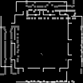
First, we consider the case where we add the same Gaussian noise to the agent’s and all objects’ positions, referenced as NOSM (player/objects), meaning that these elements are not properly positioned with respect to the static objects. Fig. 4(l) shows the results of adding that noise. The OSM map is shown on top and its noisy version is shown below. One thing to note here is that these maps have gray scale pixel values to define different abstractions and objects. This gray scaled format was used for training as discussed in the previous sections. Next, we add Gaussian noise to the positions of walls, referenced as NOSM (walls), meaning that some element that appear accessible in the 2D map cannot be reached in the real environment. Fig. 4(m) shows the results of adding that noise.
As can be seen in Fig. 3(bottom), this very high amount of noise in the 2D maps prevent the DQN framework to learn a good policy. However, it is important to note that in the worst case, the noisy version matches the performances of the baseline as the network learns to ignore it.
5.3 Reconstructed Semantic Maps (RSM)
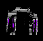
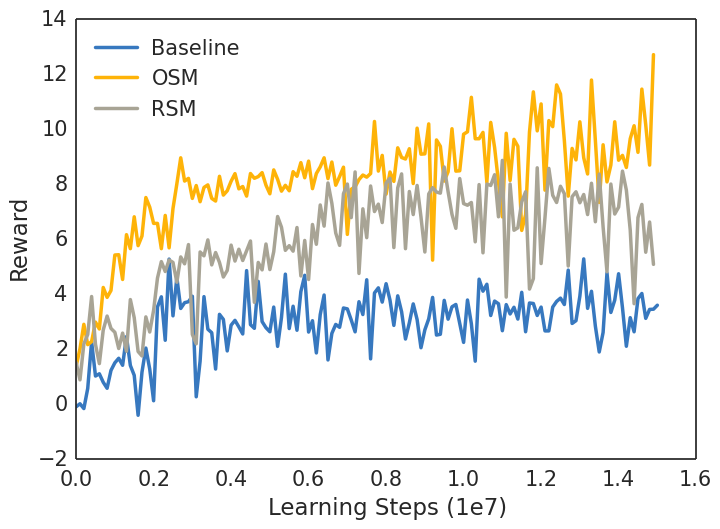
In Sec. 5.1, we have shown the efficacy of Q-learning with ground-truth version of our semantic maps. As a proof of concept, we now evaluate performance with the real maps generated on-the-fly by the approach described in Sec. 4 (RSM). This experiment allows us to evaluate the quality of the policy that can be learned when using the standard detection and mapping techniques without any extra engineering. In other words, we measure the drop in performance caused by imperfect object detection and SLAM in a real world scenario with respect to the oracle. The difference between the OSM and the RSM is seen in Fig. 4(r). Here, the semantic categories are coloured instead of greyscale levels for emphasis.
As seen in Fig. 5(l), the reconstructed map leads to significantly better results than the baseline. Even though it doesn’t match the oracle, we clearly see that the RSM is much closer to the OSM than the baseline. The remaining gap can be further reduced with progress in the field.
 |
 |
 |
5.4 Prioritized Duel DQN
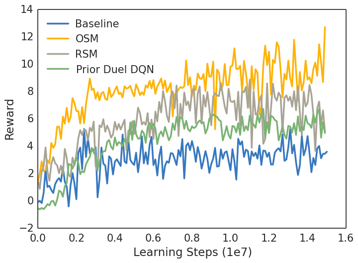
Combination of the prioritized experience replay [40] and dueling network architecture [46] has demonstrated superior results on 57 Atari games (2D environment) compared to the vanilla DQN approach that is the baseline considered above. In this experiment, we compare this successful model (referred as dDQN) with the basic DQN model augmented with our semantic maps.
Fig. 5(m) shows that while the combination of PRL with dual DQN achieves better results than the DQN baseline, the model with our semantic maps, despite trained with the basic DQN, outperformed the PRL with dual DQN trained on first person views. It is also interesting to note that these two approaches are orthogonal and could be combined. We leave this study for the future work.
5.5 Mean Run Length
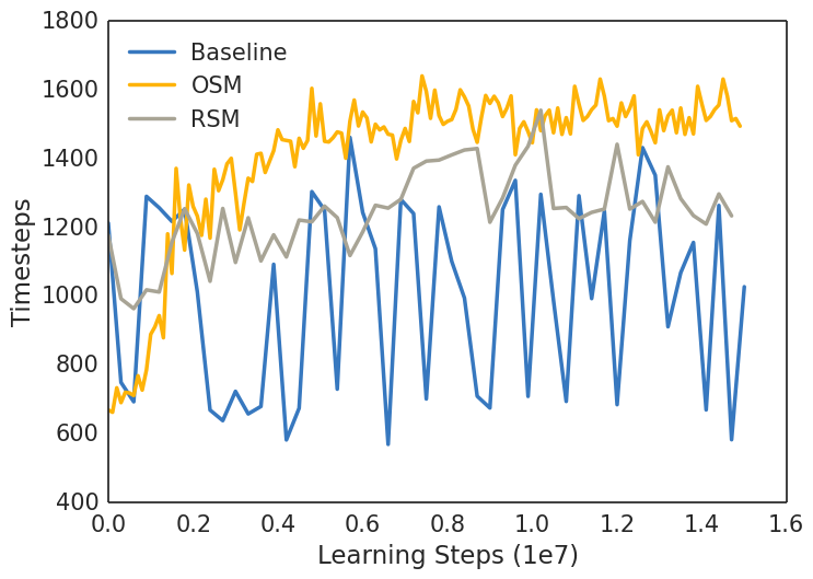
As can be seen in Fig. 5(r), the agent trained with semantic maps is able to typically live longer than the one trained only on the first-person view. This is a consequence of the fact that the OSM agent inherently attempts to build a representation of the environment it is in, which helps it adapt better from arbitrary initialisation points. The baseline however, does not have access to such capabilities, and hence performs incoherently in these situations. In keeping with the general characteristics of the results seen thus far, the RMS agent typically underperforms in relation to the ORM agent, but still significantly outperforms the baseline.
6 Discussion and Conclusion
We proposed to augment the standard DQN model with semantic maps; a representation that provides aggregated information about the 3D environment around the agent. We have demonstrated the efficacy of our approach with both oracle maps, and automatically reconstructed maps using object detection and SLAM, demonstrating the efficacy of our approach with standard computer-vision recognition and reconstruction pipeline (e.g., for road scene understanding [43]) and a standard off-the-shelf policy learner (DQN).
Our central thesis is exploring the benefits of semantic representations augmenting the directly-from-pixels learning approach typically employed. While we do not claim major contributions to policy-learning algorithms themselves, the effort nonetheless provides insight on the efficacy of such representations against those learned in a purely bottom-up manner. It also potentially serves as a benchmark for effectiveness of representations learned in a purely bottom-up manner. Moreover, our approach has the potential to extend and scale beyond the Doom environment by virtue of its applicability to any environment with a reasonable number of potential other entities and the extractability of 3D information.
In terms of future directions, we would like to extend our framework along a variety of different axes. One particular direction is improving our resilience to layered environments as we are currently unable to represent environments such as buildings (“stacked floors/levels”). Another direction involves relaxing the metric constraints that our maps are currently constructed under. Better localisation and semantic representations could exist that do not necessarily require metric reconstruction, but perhaps a more relativistic, graph-based approach. And finally, we are interested in extending our experiments to incorporate more maps (beyond the deathmatch scenario we currently employ), and elicit qualitative judgments of the learned gameplay.
References
- [1] A. G. Barto and S. Mahadevan. Recent advances in hierarchical reinforcement learning. Discrete Event Dynamic Systems, 13(4):341–379, 2003.
- [2] P. J. Besl and N. D. McKay. A method for registration of 3-d shapes. T-PAMI, 1992.
- [3] C. Bibby. Probabilistic Methods for Enhanced Marine Situational Awareness. PhD thesis, University of Oxford, 2010.
- [4] N. Burgess. Spatial cognition and the brain. Annals of the New York Academy of Sciences, 1124(1):77–97, 2008.
- [5] M. Cummins. Probabilistic Localization and Mapping in Appearance Space. PhD thesis, University of Oxford, 2009.
- [6] A. J. Davison, I. D. Reid, N. D. Molton, and O. Stasse. Monoslam: Real-time single camera slam. T-PAMI, 2007.
- [7] M. Denis and J. M. Loomis. Perspectives on human spatial cognition: memory, navigation, and environmental learning. Psychological Research, 71(3):235–239, 2007.
- [8] A. Dosovitskiy and V. Koltun. Learning to act by predicting the future. ICLR-2017 submission, 2016.
- [9] D. Eigen, C. Puhrsch, and R. Fergus. Depth map prediction from a single image using a multi-scale deep network. In NIPS. 2014.
- [10] J. Engel, T. Schöps, and D. Cremers. LSD-SLAM: Large-scale direct monocular SLAM. In ECCV, 2014.
- [11] P. F. Felzenszwalb, R. B. Girshick, D. A. McAllester, and D. Ramanan. Object detection with discriminatively trained part-based models. T-PAMI, 2010.
- [12] M. A. Fischler and R. C. Bolles. Random sample consensus: A paradigm for model fitting with applications to image analysis and automated cartography. Commun. ACM, 1981.
- [13] M. A. Fischler and R. A. Elschlager. The representation and matching of pictorial structures. T-Computers, 1973.
- [14] D. J. Freedman and E. K. Miller. Neural mechanisms of visual categorization: insights from neurophysiology. Neuroscience & Biobehavioral Reviews, 32(2):311–329, 2008.
- [15] R. Girshick. Fast R-CNN. ICCV, 2015.
- [16] R. Girshick, F. Iandola, T. Darrell, and J. Malik. Deformable part models are convolutional neural networks. In CVPR, 2015.
- [17] M. Hausknecht and P. Stone. Deep recurrent q-learning for partially observable mdps. arXiv preprint arXiv:1507.06527, 2015.
- [18] M. Hausknecht and P. Stone. Deep recurrent q-learning for partially observable mdps. arXiv preprint arXiv:1507.06527, 2015.
- [19] J. Hosang, R. Benenson, P. Dollar, and B. Schiele. What makes for effective detection proposals? T-PAMI, 2016.
- [20] W. Jaśkowski, M. Kempka, M. Wydmuch, and J. Toczek. Vizdoom competition.
- [21] M. Kempka, M. Wydmuch, G. Runc, J. Toczek, and W. Jaśkowski. Vizdoom: A doom-based ai research platform for visual reinforcement learning. arXiv preprint arXiv:1605.02097, 2016.
- [22] G. Klein and D. W. Murray. Parallel tracking and mapping for small ar workspaces. In ISMAR, 2007.
- [23] R. Kuemmerle, G. Grisetti, H. Strasdat, K. Konolige, and W. Burgard. g2o: A general framework for graph optimization. In ICRA, 2011.
- [24] T. D. Kulkarni, K. R. Narasimhan, A. Saeedi, and J. B. Tenenbaum. Hierarchical deep reinforcement learning: Integrating temporal abstraction and intrinsic motivation. arXiv preprint arXiv:1604.06057, 2016.
- [25] G. Lample and D. S. Chaplot. Playing fps games with deep reinforcement learning. arXiv preprint arXiv:1609.05521, 2016.
- [26] V. Lepetit, F. Moreno-Noguer, and P. Fua. Epnp: An accurate o(n) solution to the pnp problem. IJCV, 2009.
- [27] S. Liwicki, C. Zach, O. Miksik, and P. H. S. Torr. Coarse-to-fine planar regularization for dense monocular depth estimation. In ECCV, 2016.
- [28] M. J. Milford, G. F. Wyeth, and D. Prasser. Ratslam: a hippocampal model for simultaneous localization and mapping. In ICRA, 2004.
- [29] V. Mnih, K. Kavukcuoglu, D. Silver, A. Graves, I. Antonoglou, D. Wierstra, and M. Riedmiller. Playing atari with deep reinforcement learning. In NIPS Deep Learning Workshop. 2013.
- [30] V. Mnih, K. Kavukcuoglu, D. Silver, A. A. Rusu, J. Veness, M. G. Bellemare, A. Graves, M. Riedmiller, A. K. Fidjeland, G. Ostrovski, et al. Human-level control through deep reinforcement learning. Nature, 2015.
- [31] E. I. Moser, E. Kropff, and M.-B. Moser. Place cells, grid cells, and the brain’s spatial representation system. Annual Review of Neuroscience, 31(1):69–89, 2008.
- [32] R. Mur-Artal, J. M. M. Montiel, and J. D. Tardós. ORB-SLAM: a versatile and accurate monocular SLAM system. T-RO, 2015.
- [33] R. A. Newcombe, S. Izadi, O. Hilliges, D. Molyneaux, D. Kim, A. J. Davison, P. Kohli, J. Shotton, S. Hodges, and A. Fitzgibbon. Kinectfusion: Real-time dense surface mapping and tracking. In ISMAR, 2011.
- [34] R. A. Newcombe, S. Lovegrove, and A. J. Davison. Dtam: Dense tracking and mapping in real-time. In ICCV, 2011.
- [35] M. Nießner, M. Zollhöfer, S. Izadi, and M. Stamminger. Real-time 3d reconstruction at scale using voxel hashing. ACM TOG, 2013.
- [36] S. Ren, K. He, R. Girshick, and J. Sun. Faster R-CNN: Towards real-time object detection with region proposal networks. T-PAMI, 2015.
- [37] E. Rosten, R. Porter, and T. Drummond. Faster and better: A machine learning approach to corner detection. T-PAMI, 2010.
- [38] E. Rublee, V. Rabaud, K. Konolige, and G. R. Bradski. Orb: An efficient alternative to sift or surf. In ICCV, 2011.
- [39] O. Russakovsky and et al. ImageNet Large Scale Visual Recognition Challenge. IJCV, 2015.
- [40] T. Schaul, J. Quan, I. Antonoglou, and D. Silver. Prioritized experience replay. Advances in ICLR, 2016.
- [41] J. Stühmer, S. Gumhold, and D. Cremers. Real-time dense geometry from a handheld camera. In DAGM, 2010.
- [42] R. S. Sutton, D. Precup, and S. Singh. Between mdps and semi-mdps: A framework for temporal abstraction in reinforcement learning. AI, 112(1):181–211, 1999.
- [43] V. Vineet, O. Miksik, M. Lidegaard, M. Nießner, S. Golodetz, V. A. Prisacariu, O. Kähler, D. W. Murray, S. Izadi, P. Perez, and P. H. S. Torr. Incremental dense semantic stereo fusion for large-scale semantic scene reconstruction. In ICRA, 2015.
- [44] P. Viola and M. J. Jones. Robust real-time face detection. IJCV, 2004.
- [45] C.-C. Wang, C. Thorpe, S. Thrun, M. Hebert, and H. Durrant-Whyte. Simultaneous localization, mapping and moving object tracking. IJRR, 2007.
- [46] Z. Wang, T. Schaul, M. Hessel, H. van Hasselt, M. Lanctot, and N. de Freitas. Dueling Network Architectures for Deep Reinforcement Learning. arXiv preprint arXiv:1511.06581, 2016.
- [47] M. D. Zeiler and R. Fergus. Visualizing and understanding convolutional networks. In ECCV, 2014.
