Equilibration in one-dimensional quantum hydrodynamic systems

Dedicated to John Cardy on the occasion of his 70th birthday

Abstract We study quench dynamics and equilibration in one-dimensional quantum hydrodynamics, which provides effective descriptions of the density and velocity fields in gapless quantum gases. We show that the information content of the large time steady state is inherently connected to the presence of ballistically moving localised excitations. When such excitations are present, the system retains memory of initial correlations up to infinite times, thus evading decoherence. We demonstrate this connection in the context of the Luttinger model, the simplest quantum hydrodynamic model, and in the quantum KdV equation. In the standard Luttinger model, memory of all initial correlations is preserved throughout the time evolution up to infinitely large times, as a result of the purely ballistic dynamics. However nonlinear dispersion or interactions, when separately present, lead to spreading and delocalisation that suppress the above effect by eliminating the memory of non-Gaussian correlations. We show that, for any initial state that satisfies sufficient clustering of correlations, the steady state is Gaussian in terms of the bosonised or fermionised fields in the dispersive or interacting case respectively. On the other hand, when dispersion and interaction are simultaneously present, a semiclassical approximation suggests that localisation is restored as the two effects compensate each other and solitary waves are formed. Solitary waves, or simply solitons, are experimentally observed in quantum gases and theoretically predicted based on semiclassical approaches, but the question of their stability at the quantum level remains to a large extent an open problem. We give a general overview on the subject and discuss the relevance of our findings to general out of equilibrium problems.

I Introduction

A decade ago Calabrese and Cardy CC_QQ introduced the concept of quantum quench as a generic physical setup for the study of universal features in out-of-equilibrium quantum statistical physics. Together with a profound conjecture for the large time steady state in integrable models, the Generalised Gibbs Ensemble (GGE) of Rigol et al. Rigol_GGE proposed in the same year, these two concepts have been highly inspiring, especially as a means to understand the mechanism of equilibration in closed quantum systems Eisert ; s-jstat1 ; s-jstat2 ; s-jstat3 ; Bernard-Doyon ; QA2 ; s-jstat6 ; quasi-local2 ; s-jstat7 . Interestingly, the celebrated first experimental observation of a GGE that was only recently achieved exp:GGE brings back the original problem considered in CC_QQ , that of the quantum dynamics in a one-dimensional (1D) gapless system.

Perhaps the most intriguing problem regarding equilibration in quantum systems is the mechanism of memory loss: Let us consider an extended quantum system prepared in a general initial state and let it evolve under unitary dynamics over a long time. Would it relax locally to a statistical ensemble that retains comparatively little memory of the initial state? What are the physical conditions and what the physical mechanism of this memory loss? What presicely is the information content of the steady state ensemble for a general initial state?

Integrable models are, in this respect, an ideal testing ground of equilibration: on the one hand, they are characterised by an extensive number of conservation laws that prevent relaxation to a thermal ensemble; on the other hand, their exact solvability allows the ab initio study of their dynamics, thus offering us the opportunity to identify the physical principles behind memory loss and memory preservation in out-of-equilibrium quantum systems. What the GGE conjecture essentially postulates is that, while such integrable systems do not thermalise, they still equilibrate locally but to an ensemble that contains information about their extra conservation laws. Even though it is still unclear which conserved quantities should be included in the general case, in its currently most complete form GGEfail1 ; GGEfail2 ; completeGGE the GGE is defined through the information of the distribution densities of distinct types of initial excitations, which amounts to including both local and the recently discovered quasi-local conserved charges quasi-local ; quasi-local2 . Despite the fact that the number of such charges in a thermodynamically large system is infinite, this is still an enormously economic ensemble: While a complete description of local observables in a general initial state would require knowledge of each multi-point correlation function separately, or equivalently, of the amplitudes of clusters of excitations of any order cluster , the above ensemble contains information only about the distribution densities of excitations. Therefore relaxation to the GGE is associated with an enormous memory loss, from an initial information content that scales exponentially with the system size to just linear scaling in the final state. This memory loss effect is expected to be a consequence of dephasing due to the destructive interference of quasiparticles originating from very distant initially points. From this perspective gapless systems are somewhat special: the absence of an energy gap means that there is no stationary phase point, which is the most common cause of dephasing.

While the GGE conjecture has been verified in a large number of quantum quenches, the general conditions for its validity, the set of conserved charges it must generally contain and more importantly a deeper understanding of its success, are still missing. One approach to prove it from first principles of quantum many-body physics relates it to two precise and broadly applicable physical conditions, one for the initial state and one for the dynamics Cramer-Eisert ; Cramer-Eisert_b ; SC_GGE-val ; FE_cluster-dec ; S15 ; doyon ; Eisert16 . For the initial state the key factor is the clustering of correlations of local fields, a rather general property of quench initial states as a consequence of the locality of the pre-quench Hamiltonian. The role of initial clustering in equilibration was first demonstrated in Cramer-Eisert_b in the context of non-interacting lattice models, where it was shown that any initial state that satisfies the cluster property relaxes locally to a Gaussian GGE. The loss of memory is clearly reflected in the fact that a general non-Gaussian initial state relaxes to a Gaussian one that is completely determined by the knowledge of its two point correlation function. Apart from initial clustering, the proof relied also on the presence of a maximum velocity of propagation, as rigorously expressed by the Lieb-Robinson bound of lattice systems with finite-range couplings LR . This approach has been recently extended to the far more general case of genuinely interacting lattice systems with finite-range couplings, including non-integrable ones doyon . In the context of continuous field theories, the importance of the cluster property was rediscovered in SC_GGE-val . The existence of a maximum group velocity of excitations is by default a property of relativistic quantum field theories, but it turned out that it is not a necessary condition for the validity of the GGE, since the same conclusion was reached also in a non-relativistic bosonic system. On the other hand, in S15 it was shown that when the evolution follows a free massless relativistic field theory, despite the inherent light-cone dynamics, the equilibrium state is not described by a Gaussian GGE, as memory of all initial correlation functions is preserved up to infinite time. Back to the lattice, a new perspective on the equilibration mechanism was introduced in Eisert16 by unveiling a link to transport properties. It was discovered that a sufficient condition on the dynamics is that the evolution Hamiltonian exhibits delocalised transport, i.e. spreading of initially localised wavepackets such that they decay with time uniformly in the whole space. Even though all above results, with the exception of doyon , were demonstrated under the assumption of essentially non-interacting dynamics, the conclusions of doyon suggest that they naturally extend to the interacting case.

The condition of delocalised transport can be easily understood intuitively: if the time evolution follows a Hamiltonian characterised by localisation, then the initial state and its correlations practically “freeze” and do not evolve significantly theor:MBL-dynamics . In fact this effect was exploited for the experimental observation of many body localisation induced by disorder exp:MBL . Though seemingly contraddictory, a not so different type of localisation occurs also in systems that exhibit purely ballistic transport: those for which the Heisenberg equations of motion admit ballistically moving localised solutions. Gapless relativistically invariant systems described by the standard Luttinger model with linear dispersion are the simplest examples of such type of transport. Due to the purely ballistic nature of transport, entangled clusters of left or right-moving particle excitations of the initial state are parallel transported throughout the time evolution, carrying their initial correlations intact up to infinite times S15 .

The demonstration of the above memory effect in the Luttinger model relies on its gaplessness and relativistic invariance. While this model has been argued to provide a good description of the dynamics in relevant cold atom experiments exp:lightcone1 ; exp:lightcone2 , the ultimate fate of this memory effect depends on whether deviations of physical systems from the Luttinger model undermine the stability of such ballistic localised excitations. The most important deviations in quantum gases are the nonlinear dispersion and the presence of interactions that are not captured by the standard Luttinger model nonlinear_LL1 ; nonlinear_LL . We show that each of these features, when considered separately, breaks the purely ballistic character of the dynamics, leading to spreading of wavepackets and delocalisation. Due to this effect, in analogy with Eisert16 we show that in both of these cases equilibration is characterised by memory loss and the steady state is a Gaussian GGE in terms of a suitable choice of fields. On the other hand, in the presence of both dispersion and interactions their combined effect opens up another possibility: Let us recall that in classical integrable models solitary waves, or simply solitons, emerge as the result of mutual cancellation between dispersion and interaction and notice that solitary waves are characterised by precisely the features we have identified as leading to memory preservation, i.e. ballistic transport and localisation. As observed in GP-solitons ; classical_soliton-quench , we find that a semiclassical approach would suggest that such solitons emerge and restore the ballistic localised character of the dynamics, raising the question whether this type of behaviour persists when quantum fluctuations are taken into account.

This brings to the forefront the emerging field of 1D quantum hydrodynamics q_hydrodyn1 ; QH0 ; QH1 ; QH2 ; QH3 ; QH4 ; GP-solitons_long ; q_hydrodyn2 ; Bernard-Doyon2 and, as a prototype model, the quantum Korteweg-de Vries (KdV) equation qKdV-LL ; qKdV1 ; qKdV2 ; GP-solitons ; GP-solitons_long , which is expected to capture the leading deviations from Luttinger model that are relevant to the dynamics of 1D Bose gases qKdV-LL ; GP-solitons . Experiments in 1D cold atomic gases have achieved the observation of dispersionless bright solitons exp:bright_soliton and the formation and propagation of soliton trains exp:soliton_train in the case of attractive interaction, as well as dark solitons that eventually disperse in the case of repulsive interactions exp:dark_soliton . The existence of solitons in such quantum gases has been theoretically predicted by means of the semiclassical approach, using the Gross-Pitaevski or Non-Linear Schrödinger Equation (NLSE) theor:solitons_NLS , the KdV KdV_solution ; ZK and the Benjamin-Ono equation B-O , all of which admit classical soliton solutions. Stable soliton solutions have been argued to persist at the quantum level in the quantum Benjamin-Ono equation q_hydrodyn1 , which is the hydrodynamic description of the Calogero-Sutherland model, confirming in this way earlier predictions Jevicki ; soliton_calogero ; soliton_calogero2 . These findings are evidence of the existence of solitary waves in quantum hydrodynamic systems, whose presence in different models remains however an open problem. More specifically, in the repulsive Lieb-Liniger model, whose low-energy effective hydrodynamic description is given by the quantum KdV equation, the semiclassical approach in combination with Bethe-Ansatz analysis suggests that the solitons become unstable and disperse at large times, even though with a weaker dispersion law than the phononic excitations qKdV-LL . In this model it has been conjectured that static dark solitons can be formed out of Lieb’s type-II excitations dark-solitons-Lieb2 ; classical-quantum_NLSE and numerical results seem to confirm this conjecture, although they are not yet conclusive about their dynamical stability ds_debate1 ; dark_soliton_debate1 ; ds_debate2 ; deguchi . In the context of quenches, the KdV and NLSE equations have been used for the study of dynamics of a soliton undergoing an interaction quench GP-solitons ; GP-solitons_long .

Coming back to the problem of determining the steady state’s information content, we realise that the crucial question that arises is if the long time asymptotics of the (operatorial now) solution of the equations of motion involves solitary waves. In such case, memory of all initial soliton correlations survives in the steady state. Systems exhibiting quantum solitary waves can therefore evade decoherence and the memory loss typically associated with the equilibration process, yet exhibiting non-trivial dynamics without the local freezing of disorder-induced localisation. These features make quantum solitons perfect candidates for applications to quantum communication and quantum information processing in many-body systems, for which reason their dynamics, collisions and entanglement properties have been the subject of recent studies entanglement_q-solitons ; entangl ; entangl_2 ; entangl_3 ; soliton_dyn ; soliton_qdyn ; Bell-states ; coll_dyn . Motivated by the semiclassical approximation to the quantum KdV equation, it is tempting to give a positive answer to the above question: the general solution to the classical KdV equation for an arbitrary initial condition always decomposes into a finite number of solitons and a decaying dispersive component math:KdV_asympt . In fact it was exactly the observation of solitons in the classical KdV equation by Zabusky and Kruskal that led them to the explanation of the absence of ergodicity in the Fermi-Pasta-Ulam problem in their seminal work ZK . However, this semiclassical argument is insufficient in order to address the above question in the quantum case, as it ignores the effects of quantum fluctuations on the soliton stability.

In this work we study the large time correlation functions of the density and velocity or phase field after a quench in a 1D Bose gas using its quantum hydrodynamic description. We first introduce the various effective theories (Sec. II), starting with the Luttinger model and extending it to the quantum KdV model by including dispersion and chiral interaction terms. We then show that time evolution following the standard Luttinger model preserves the memory of all initial correlation functions (Sec. III), while dispersion (Sec. IV) or interaction (Sec. V) considered separately lead to delocalisation which suppresses this effect: Under the condition of sufficient initial clustering, the steady state is in both cases a Gaussian GGE in terms of the bosonisation fields or the dual fermion field respectively. The main results of our analysis are two scaling relations for the time decay of corrections to the steady state values of correlation functions, which are deduced as a combination of the scaling of the initial clustering and of the dynamical spreading. In the dispersive case such a scaling relation for exponential initial clustering is given in Eq. (47), while in the interacting case it is expressed as an upper bound in Eq. (66). Next, we show that the semiclassical approximation to the quantum KdV equation suggests that the combination of dispersion and interaction restores localisation through the emergence of solitary waves (Sec. VI) and, provided that the latter persist at the quantum level, memory of soliton correlation functions is preserved at large times (Sec. VII). Lastly, we discuss the implications of our analysis (Sec. VIII) and identify open questions for future investigation (Sec. IX).

II Quantum Hydrodynamics and the Quantum KdV Equation

We are interested in the dynamics of 1D non-relativistic quantum gases, which are realised in cold atom experiments like the quasi-condensate splitting experiments in which the first observation of a GGE was achieved exp:GGE . We present quantum hydrodynamics descriptions of such systems in terms of the density and phase fields in the thermodynamic limit. We first introduce the standard bosonisation approach Haldane i.e. the Luttinger model, which is essentially a free massless relativistic field theory effectively describing the low-energy limit of such systems. We then introduce the quantum KdV equation as a nonlinear extension of the Luttinger model that incorporates effects of dispersion and interactions of the bosonised fields qKdV-LL . In particular we discuss arguments that have been used to justify this effective description in the context of out-of-equilibrium physics and in particular quantum quenches.

We consider an interacting non-relativistic Bose gas in 1D generally described by the Hamiltonian

$$\hat{H}=\int dx\,\partial_{x}\hat{\Psi}^{\dagger}(x)\partial_{x}\hat{\Psi}(x)+\int dxdx^{\prime}\,V(x-x^{\prime})\hat{\Psi}^{\dagger}(x)\hat{\Psi}(x)\hat{\Psi}^{\dagger}(x^{\prime})\hat{\Psi}(x^{\prime})$$ (1)

We have set the boson mass to $1/2$ and fix the number of particles $\hat{N}=\int dx\,\hat{\Psi}^{\dagger}(x)\hat{\Psi}(x)$. In the case of contact interaction this reduces to the integrable Lieb-Liniger Hamiltonian

$$\hat{H}_{LL}=\int dx\,\left(\partial_{x}\hat{\Psi}^{\dagger}\partial_{x}\hat{\Psi}+c\hat{\Psi}^{\dagger}\hat{\Psi}^{\dagger}\hat{\Psi}\hat{\Psi}\right)$$ (2)

Bosonisation and more general quantum hydrodynamics arise when the boson field operator $\hat{\Psi}$ is expressed in terms of the dual density and phase fields $\hat{\rho}$ and $\hat{\phi}$

$$\hat{\Psi}^{\dagger}(x)=\sqrt{\hat{\rho}(x)}\mathrm{e}^{-\mathrm{i}\hat{\phi}(x)}$$ (3)

satisfying canonical commutation relations $[\hat{\rho}(x),\hat{\phi}(x^{\prime})]=\mathrm{i}\delta(x-x^{\prime})$. The original Hamiltonian $\hat{H}$ is then written as

$$\hat{H}=\int dx\,\left[\hat{\rho}\left(\partial_{x}\hat{\phi}\right)^{2}+\tfrac{1}{4}\hat{\rho}^{-1}\left(\partial_{x}\hat{\rho}\right)^{2}\right]+\int dxdx^{\prime}\,V(x-x^{\prime})\hat{\rho}(x)\hat{\rho}(x^{\prime})$$ (4)

In order to focus on the fluctuations of the density about its mean value $\rho_{0}=N/L$ we set, following Haldane Haldane

$$\hat{\rho}(x)=\rho_{0}+\frac{1}{\pi}\partial_{x}\hat{\theta}(x)$$ (5)

where the new field $\hat{\theta}(x)$ satisfies the commutation relations

$$[\partial_{x}\hat{\theta}(x),\hat{\phi}(x^{\prime})]=-[\hat{\theta}(x),\partial_{x^{\prime}}\hat{\phi}(x^{\prime})]=\mathrm{i}\pi\delta(x-x^{\prime})$$ (6)

In the bosonised description, local observables correspond to exponentials of the fields $\hat{\phi}$ and $\hat{\theta}$, the “vertex operators”, or their derivatives. Vertex operators correspond to the original boson field $\hat{\Psi}$, while derivatives correspond to the density and current density operators

$$\hat{\rho}(x) =\hat{\Psi}^{\dagger}(x)\hat{\Psi}(x)=\rho_{0}+\frac{1}{\pi}\partial_{x}\hat{\theta}(x)$$ (7)

$$\hat{j}(x) =-\frac{\mathrm{i}}{2}\left(\hat{\Psi}^{\dagger}(x)\partial_{x}\hat{\Psi}(x)-\partial_{x}\hat{\Psi}^{\dagger}(x)\hat{\Psi}(x)\right)=\sqrt{\hat{\rho}(x)}\left(\partial_{x}\hat{\phi}(x)\right)\sqrt{\hat{\rho}(x)}\sim\rho_{0}\partial_{x}\hat{\phi}(x)$$ (8)

Substituting to the above Hamiltonian and expanding in powers of $\partial_{x}\hat{\theta}$, we obtain low energy effective Hamiltonians for the system. The simplest low energy description is given by the standard Luttinger model Hamiltonian

$$\hat{H}_{Lm}=\frac{v}{2\pi}\int dx\,\left[K\left(\partial_{x}\hat{\phi}\right)^{2}+\frac{1}{K}\left(\partial_{x}\hat{\theta}\right)^{2}\right]$$ (9)

with $v=2\rho_{0}\sqrt{\gamma}$ the sound velocity, $K=\pi/\sqrt{\gamma}$ the Luttinger liquid parameter and $\gamma=c/\rho_{0}$ the dimensionless interaction strength.

It is convenient to introduce the left and right-moving chiral fields, respectively $\hat{\varphi}_{+}$ and $\hat{\varphi}_{-}$, in terms of which the Hamiltonian decouples. These are defined by

$$\hat{\varphi}_{\pm}=\frac{1}{\sqrt{K}}\hat{\theta}\mp\sqrt{K}\hat{\phi}$$ (10)

and their commutation relations are therefore

$$[\hat{\varphi}_{\sigma}(x),\partial_{x^{\prime}}\hat{\varphi}_{\sigma^{\prime}}(x^{\prime})]=2\sigma\pi\mathrm{i}\delta_{\sigma\sigma^{\prime}}\delta(x-x^{\prime})$$ (11)

We also define the rescaled bosonisation fields

$$\hat{\vartheta} =\frac{1}{2}\left(\hat{\varphi}_{+}+\hat{\varphi}_{-}\right)=\frac{1}{\sqrt{K}}\hat{\theta}$$ (12)

$$\hat{\varphi} =\frac{1}{2}\left(-\hat{\varphi}_{+}+\hat{\varphi}_{-}\right)=\sqrt{K}\hat{\phi}$$ (13)

In terms of these fields the Luttinger model Hamiltonian reads

$$\hat{H}_{Lm}=\frac{v}{4\pi}\sum_{\sigma=\pm}\int dx\,\left(\partial_{x}\hat{\varphi}_{\sigma}\right)^{2}=\frac{v}{2\pi}\int dx\,\left[\left(\partial_{x}\hat{\varphi}\right)^{2}+\left(\partial_{x}\hat{\vartheta}\right)^{2}\right]$$ (14)

Deviations from the standard Luttinger model can be taken into account by including higher order terms in the expansion of field derivatives. To determine the leading corrections that are relevant at equilibrium, one would typically apply Renormalisation Group theory arguments regarding the relevance of perturbative corrections. While these arguments are justified for the study of ground or thermal state physics, in the context of quenches higher energy excitations need also to be taken into account. This can be done to first order by including terms of the next-to-leading scaling dimension qKdV-LL . On the other hand, non-chiral contributions to the Hamiltonian can be neglected to first approximation. Such terms are expected to induce a modification of the velocity of the chiral excitations Cardy ; Bernard-Doyon2 .

Under the above assumptions, we include only chiral terms of scaling dimension three or four, thus obtaining the Hamiltonian

$$\hat{H}=\hat{H}_{Lm}+\hat{H}_{KdV}$$ (15)

where $\hat{H}_{KdV}$ is the quantum KdV Hamiltonian

$$\hat{H}_{KdV}=\frac{1}{4\pi}\sum_{\sigma=\pm}\int dx\,\left[\alpha\left(\partial_{x}\hat{\varphi}_{\sigma}\right)^{3}+\beta\left(\partial_{x}^{2}\hat{\varphi}_{\sigma}\right)^{2}\right]$$ (16)

with $\alpha=1/(2\sqrt{K})$ and $\beta=K/(4\pi^{2}\rho_{0})$. The first term in the above Hamiltonian

$$\hat{H}_{int}=\frac{\alpha}{4\pi}\sum_{\sigma=\pm}\int dx\,\left(\partial_{x}\hat{\varphi}_{\sigma}\right)^{3}$$ (17)

is an interaction in terms of the bosonisation fields, while the second term

$$\hat{H}_{disp}=\frac{\beta}{4\pi}\sum_{\sigma=\pm}\int dx\,\left(\partial_{x}^{2}\hat{\varphi}_{\sigma}\right)^{2}$$ (18)

is only a quadratic dispersion term.

Another convenient field transformation is introduced by the fermionisation method refermionisation ; qKdV1 ; BF . Based on the boson-fermion correspondence, introduced in the seminal works of Mattis and Mandelstam Mandelstam ; Mattis ; Coleman ; Mattis-Lieb ; Luther-Peschel , we define the fermionic quasiparticle field

$$\hat{\Phi}_{\sigma}^{\dagger}(x)=\hat{F}_{\sigma}\frac{1}{\sqrt{2\pi a}}\mathrm{e}^{2\pi\mathrm{i}\sigma\rho_{0}x}\mathrm{e}^{\mathrm{i}(\sigma\hat{\vartheta}(x)-\hat{\varphi}(x))}$$ (19)

where $\hat{F}_{\sigma}$ are the Klein factors and $a$ a short distance cutoff (or lattice spacing in lattice model applications). Using this transformation the Luttinger model Hamiltonian can be written as a free fermion Hamiltonian with linear dispersion

$$\hat{H}_{Lm}=-\mathrm{i}v\sum_{\sigma=\pm}\sigma\int dx\,:\hat{\Phi}_{\sigma}^{\dagger}(x)\partial_{x}\hat{\Phi}_{\sigma}(x):$$ (20)

where $:\,:$ denotes normal ordering in terms of the fermions. Moreover, the bosonic interaction term of the quantum KdV Hamiltonian can be written as a free fermionic dispersion term qKdV1 ; qKdV-LL ; refermionisation

$$\hat{H}_{int}=\frac{1}{2m_{*}}\sum_{\sigma=\pm}\int dx\,:{\left(\partial_{x}\hat{\Phi}_{\sigma}^{\dagger}\right)\left(\partial_{x}\hat{\Phi}_{\sigma}\right)}:$$ (21)

with $m_{*}\propto 1/\alpha$ the effective fermion mass.

We notice that the quantum KdV Hamiltonian contains only terms which are quadratic in either the bosonised or the fermion fields qKdV1 ; qKdV2 . In particular if the bosonic interaction term is absent ($\alpha=0$) the Hamiltonian is free in terms of the bosonised fields, while if the dispersion term is absent ($\beta=0$) the Hamiltonian is free in terms of the fermionic field. The various Hamiltonian terms and their physical meaning in terms of the three field theoretic descriptions, the original boson field, the density and phase fields and the fermionic quasiparticle field, are summarised in Table 1. In particular, non-linear dispersion of the bosonisation fields arises as a result of an inter-particle interaction that is not of local (point-like) type, but non-local, or from the inclusion of next-to-leading order terms in the expansion of the kinetic energy part of the Hamiltonian. On the other hand, interaction of the bosonised fields arises as a result of the non-linear (non-relativistic) dispersion of the original bosonic particles. More details on this correspondence can be found in nonlinear_LL and a discussion of their role on dynamics in qKdV-LL .

original bosons/fermions $\hat{\Psi}^{\dagger}$	bosonisation fields $\hat{\phi},\hat{\theta}$		fermionic quasiparticles $\hat{\Phi}^{\dagger}$
local interaction	free	linear dispersion	free	linear disp.
non-local interaction		non-linear dispersion	interacting	interaction + nl. disp.
kinetic energy (next-to-leading order corrections)
non-linear dispersion / band curvature	interacting	non-chiral interaction		irrelevant interaction
		chiral interaction	free	non-linear disp.

Table 1: The dictionary of Luttinger liquids.

III Time Evolution in the Luttinger Model

We derive the long time limit of correlation functions for the density and phase fields assuming that the evolution follows the standard Luttinger model, i.e. the free massless and relativistic boson Hamiltonian. We will see that, due to the purely ballistic time evolution of the fields, dephasing is suppressed and the initial correlations are preserved intact up to infinite times, with no memory loss. The only mixing of information that takes place is the averaging between the left and right-moving chiral modes. Moreover tracking the initial origin of the information that survives at large times we see that it is located at the two spatial infinities. Therefore the large time correlations are independent of initial correlations in any finite part in the middle. These features are characteristics of the linear dispersion relation of the model.

The Heisenberg equations of motion corresponding to the standard Luttinger model Hamiltonian (9), (14) are

$$\partial_{t}\hat{\phi} =-\frac{v}{K}\partial_{x}\hat{\theta}$$ (22)

$$\partial_{t}\hat{\theta} =-vK\partial_{x}\hat{\phi}$$ (23)

or, in decoupled form in terms of the chiral fields (10),

$$\partial_{t}\hat{\varphi}_{\pm}=\pm v\partial_{x}\hat{\varphi}_{\pm}$$ (24)

which are simply equivalent forms of the wave equation in one dimension $\partial_{t}^{2}\hat{\phi}=v^{2}\partial_{x}^{2}\hat{\phi}$, with the same equation for the field $\hat{\theta}$. Its general solution for any initial field configuration, defined by the initial conditions $\hat{\phi}(x,0)$ and $\partial_{t}\hat{\phi}(x,0)=-\frac{v}{K}\partial_{x}\hat{\theta}(x,0)$, is given by d’Alembert’s formula

$$\hat{\phi}(x,t) =\frac{1}{2}\left(\hat{\phi}(x-vt,0)+\hat{\phi}(x+vt,0)\right)+\frac{1}{2v}\int_{x-vt}^{x+vt}dx^{\prime}\,\partial_{t}\hat{\phi}(x^{\prime},0)$$

$$=\frac{1}{2}\left(\hat{\phi}(x-vt,0)+\hat{\phi}(x+vt,0)\right)+\frac{1}{2K}\left(\hat{\theta}(x-vt,0)-\hat{\theta}(x+vt,0)\right)$$

$$=-\frac{1}{2\sqrt{K}}\sum_{\sigma=\pm}\sigma\partial_{x}\hat{\varphi}_{\sigma}(x+\sigma vt,0)$$ (25)

We are interested however in the values of local observables at long times, which as explained above correspond to vertex operators or derivatives of the bosonisation fields. For simplicity here we focus on density fluctuations, which are given in terms of the rescaled field (12) by the derivative $\partial_{x}\hat{\vartheta}$. Its time evolution is given by

$$\partial_{x}\hat{\vartheta}(x,t) =\frac{1}{2}\sum_{\sigma=\pm}\partial_{x}\hat{\varphi}_{\sigma}(x+\sigma vt,0)$$ (26)

that is, it is expressed in terms of initial local fields located at the lightcone projection points $x\pm vt$.

Having a direct relation between the time evolved local field and initial local fields, it is now easy to calculate the long time asymptotics of its correlations. The general multi-point correlation function at time $t$ is

$$\left\langle\prod_{i=1}^{n}\partial_{x}\hat{\vartheta}(x_{i},t)\right\rangle =\frac{1}{2^{n}}\left\langle\prod_{i=1}^{n}\sum_{\sigma=\pm}\partial_{x}\hat{\varphi}_{\sigma}(x_{i}+\sigma vt,0)\right\rangle=\frac{1}{2^{n}}\sum_{\{\sigma_{i}\}}\left\langle\prod_{i=1}^{n}\partial_{x}\hat{\varphi}_{\sigma_{i}}(x_{i}+\sigma_{i}vt,0)\right\rangle$$ (27)

where the expectation value refers to the initial state $|\Omega\rangle$. In the long time limit the above expectation values correspond to initial correlation functions between right chiral fields spatially located at points tending to $-\infty$ and left chiral fields at points tending to $+\infty$. Since these fields are local, by application of the cluster decomposition property of the initial state we find that as $t\to\infty$ the above correlation functions factorise to a product of two components, one for each of the spatial infinities (Fig. 1)

$$\lim_{t\to\infty}\left\langle\prod_{i=1}^{n}\partial_{x}\hat{\varphi}_{\sigma_{i}}(x_{i}+\sigma_{i}vt,0)\right\rangle =\lim_{t\to\infty}\left\langle\prod_{i:\,\sigma_{i}=-}\partial_{x}\hat{\varphi}_{-}(x_{i}-vt,0)\right\rangle\left\langle\prod_{i:\,\sigma_{i}=+}\partial_{x}\hat{\varphi}_{+}(x_{i}+vt,0)\right\rangle$$

$$=\left\langle\prod_{i:\,\sigma_{i}=-}\partial_{x}\hat{\varphi}_{-}(x_{i},0)\right\rangle_{-\infty}\quad\left\langle\prod_{i:\,\sigma_{i}=+}\partial_{x}\hat{\varphi}_{+}(x_{i},0)\right\rangle_{+\infty}$$ (28)

where the indices $\pm\infty$ refer to the asymptotic values of initial correlation functions at the respective spatial infinities. This formula is valid even if the initial state is not translationally invariant in the whole space but only asymptotically at the two spatial infinities (as in the widely studied case of a system that is initially split in two halves at different temperature or presents any type of step-like inhomogeneity Bernard-Doyon ). If instead we assume that the initial state is translationally invariant, we can drop the $\pm\infty$ indices since the expectation values at both spatial infinities are equal.

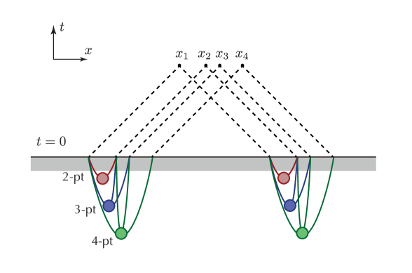
Figure 1: Diagrammatic representation of the calculation of long time correlations in the standard Luttinger model.

The above can be expressed elegantly in terms of connected correlation functions. Connected (also called ‘truncated’) correlation functions are defined as joint cumulants between local fields located at different points, i.e. they are equal to correlation functions from which all possible combinations of factorised correlations have been subtracted off. More precisely, the above definition explains the use of the term ‘truncated’, while the term ‘connected’ is justified by the linked cluster theorem, which shows that the above defined truncated correlation functions are identified with correlation functions defined through connected graphs NO . The cluster decomposition property is rephrased as decay of the connected correlation fuctions with the distance between any subset of points and the rest, and comes obviously as a direct consequence of their connectedness. Expressed in momentum space, the cluster decomposition property means that the Fourier transform of connected correlation functions can contain at most one $\delta$-function singularity that accounts for momentum conservation, i.e. translational invariance of the state, but no other such singularity Weinberg . Milder singularities, like poles or branch cuts at the real axis are instead allowed and reflect algebraically decaying correlations, as in ground states of gapless systems. If there is no singularity along the real momentum axis, but only elsewhere in the complex plane, then correlations decay exponentially as in ground states of gapped systems or in thermal states of quantum gases at non-zero temperature. A state that is Gaussian in terms of some choice of local fields, has vanishing connected correlation functions for those fields for all orders higher than two. This is a consequence of Wick’s theorem, which is valid precisely for Gaussian states.

From the above results, we find that connected correlation functions between the two distinct chiral field components vanish in the large time limit, as they originate from two different spatial infinities at initial time. Denoting connected correlation functions by double angular brackets $\mathopen{\hbox{${\langle}$}\kern-2.72221pt\leavevmode\hbox{${\langle}$}}\dots\mathclose{\hbox{${\rangle}$}\kern-2.72221pt\leavevmode\hbox{${\rangle}$}}$ and using their multi-linearity, the above result can be expressed as

$$\lim_{t\to\infty}\mathopen{\hbox{${\bigg{\langle}}$}\kern-2.72221pt\leavevmode\hbox{${\bigg{\langle}}$}}\prod_{i=1}^{n}\partial_{x}\hat{\vartheta}(x_{i},t)\mathclose{\hbox{${\bigg{\rangle}}$}\kern-2.72221pt\leavevmode\hbox{${\bigg{\rangle}}$}} =\lim_{R\to\infty}\left[\mathopen{\hbox{${\bigg{\langle}}$}\kern-2.72221pt\leavevmode\hbox{${\bigg{\langle}}$}}\prod_{i=1}^{n}\partial_{x}\hat{\varphi}_{-}(x_{i}-R)\mathclose{\hbox{${\bigg{\rangle}}$}\kern-2.72221pt\leavevmode\hbox{${\bigg{\rangle}}$}}+\mathopen{\hbox{${\bigg{\langle}}$}\kern-2.72221pt\leavevmode\hbox{${\bigg{\langle}}$}}\prod_{i=1}^{n}\partial_{x}\hat{\varphi}_{+}(x_{i}+R)\mathclose{\hbox{${\bigg{\rangle}}$}\kern-2.72221pt\leavevmode\hbox{${\bigg{\rangle}}$}}\right]$$

$$=\mathopen{\hbox{${\bigg{\langle}}$}\kern-2.72221pt\leavevmode\hbox{${\bigg{\langle}}$}}\prod_{i=1}^{n}\partial_{x}\hat{\varphi}_{-}(x_{i})\mathclose{\hbox{${\bigg{\rangle}}$}\kern-2.72221pt\leavevmode\hbox{${\bigg{\rangle}}$}}_{-\infty}+\mathopen{\hbox{${\bigg{\langle}}$}\kern-2.72221pt\leavevmode\hbox{${\bigg{\langle}}$}}\prod_{i=1}^{n}\partial_{x}\hat{\varphi}_{+}(x_{i})\mathclose{\hbox{${\bigg{\rangle}}$}\kern-2.72221pt\leavevmode\hbox{${\bigg{\rangle}}$}}_{+\infty}$$ (29)

since all other combinations of fields involve certainly both chiral components. Equivalent results have been derived in S15 and in the more general context of out of equilibrium Conformal Field Theory in Bernard-Doyon1a ; Bernard-Doyon1b .

While we have focused on field derivatives, the calculation can be easily repeated for general correlation functions of vertex operators. As shown in S15 , in the long time limit the so-called ‘neutrality condition’ is restored, which means that only correlations of chiral field differences between any point and some reference point survive. As for field derivatives, correlations between field differences originate from initial correlations at the left and right spatial infinities, therefore the same arguments apply also here.

IV The Effect of Nonlinear Dispersion

We now turn our attention to the effect of nonlinear dispersion, which is induced by terms in the Hamiltonian that involve higher spatial derivatives and are quadratic in the bosonisation fields. Considering as before the propagation of initially localised fields, we realise that nonlinear dispersion leads to spreading and consequently decay of the propagator with time. This effect, in combination with sufficient initial clustering of correlations, is responsible for the relaxation towards a Gaussian GGE in terms of the bosonised fields.

The time evolution in the present case is described by the Hamiltonian $\hat{H}_{Lm}+\hat{H}_{\text{disp}}$ with

$$\hat{H}_{\text{disp}}=\frac{\beta}{2\pi}\int dx\,\left[K\left(\partial_{x}^{2}\hat{\phi}\right)^{2}+\frac{1}{K}\left(\partial_{x}^{2}\hat{\theta}\right)^{2}\right]=\frac{\beta}{4\pi}\sum_{\sigma=\pm}\int dx\,\left(\partial_{x}^{2}\hat{\varphi}_{\sigma}\right)^{2}$$ (30)

Since this Hamiltonian is also quadratic in the bosonised fields, the time evolution can be still derived exactly. Using the commutation relations (11), the equations of motion $\partial_{t}\hat{\varphi}=i[\hat{H},\hat{\varphi}]$ can be easily shown to be

$$\partial_{t}\hat{\varphi}_{\pm}(x,t)=\pm\left(v\partial_{x}\hat{\varphi}_{\pm}(x,t)-\beta\partial_{x}^{3}\hat{\varphi}_{\pm}(x,t)\right)$$ (31)

or in terms of the field $\hat{\phi}$

$$\partial^{2}_{t}\hat{\phi}(x,t)=\left(v\partial_{x}-\beta\partial_{x}^{3}\right)^{2}\hat{\phi}(x,t)$$ (32)

and similarly for $\hat{\theta}$. The general solution to the equations of motion for any quadratic bosonic field theory is given by

$$\hat{\phi}(x,t)=\int dx^{\prime}\left(\partial_{t}G(x-x^{\prime},t)\hat{\phi}(x^{\prime},0)+G(x-x^{\prime},t)\partial_{t}\hat{\phi}(x^{\prime},0)\right)$$ (33)

where $G(x,t)$ is the (retarded) Green’s function of the equation of motion, which is

$$G(x,t)=\int\frac{dk}{2\pi}\,\mathrm{e}^{\mathrm{i}kx}\frac{\sin\omega(k)t}{\omega(k)}$$ (34)

with $\omega(k)$ the dispersion relation. One way to show the above is to express the equation of motion in momentum space, solve it for arbitrary initial conditions

$$\hat{\phi}_{k}(t)=\hat{\phi}_{k}(0)\cos\omega(k)t+\partial_{t}\hat{\phi}_{k}(0)\frac{\sin\omega(k)t}{\omega(k)}=\frac{1}{2}\sum_{\sigma=\pm 1}\left(\hat{\phi}_{k}(0)+\sigma\frac{\partial_{t}\hat{\phi}_{k}(0)}{\mathrm{i}\omega(k)}\right)\mathrm{e}^{\mathrm{i}\sigma\omega(k)t}$$ (35)

and then return to coordinate space.

In the present case, the dispersion relation is

$$\omega(k)=|k|\left(v+\beta k^{2}\right)$$ (36)

as we can easily find by substituting the general solution to the equation of motion (32). More generally, the phonon dispersion relation in gapless systems is a function of the form

$$\omega(k)=v|k|f(k)\sim v|k|+\lambda|k|^{\gamma}+...$$ (37)

where the function $f(k)$ satisfies $f(0)=1$ and is assumed to be monotonically increasing, in order to ensure that bosonisation can be applied Haldane . In the present case the first order correction to the linear dispersion is cubic i.e. $\gamma=3$ with $\lambda>0$. In non-relativistic interacting Bose gases the phonon dispersion is typically of the Bogoliubov form, whose leading low-momentum correction to the linear dispersion is precisely as in (36). However there is no fundamental reason preventing a quadratic correction i.e. $\gamma=2$: in fact this type of dispersion is encountered in the Calogero-Sutherland model whose quantum hydrodynamic field theory description is given by the Benjamin-Ono equation q_hydrodyn2 ; B-O2 . In gapless lattice models with finite range interactions, like the Ising model in transverse field, XY or XXZ models in their critical phases, we find cubic corrections with $\lambda<0$ consistently with the Lieb-Robinson bound.

For a linear dispersion relation, we set $\beta=0$ and the Green’s function is

$$G(x,t)=\int\frac{dk}{2\pi}\,\mathrm{e}^{\mathrm{i}kx}\frac{\sin v|k|t}{v|k|}=\frac{1}{2v}\Theta(vt-|x|)$$ (38)

thus we recover d’Alembert’s formula. For non-linear dispersion the Green’s function retains qualitatively its step-like form, but it is no longer sharp: it is smeared over a length that grows algebraically with time. This means in particular that field derivatives, which are those that represent local fields, are no longer simply equal to initial fields at the two light-cone projection points $x\pm vt$, but instead convolutions of initial derivative fields, centered at those points, which now spread and decay with time. More explicitly we have

$$\partial_{x}\hat{\vartheta}(x,t) =\int dx^{\prime}\left(\partial_{t}G(x-x^{\prime},t)\partial_{x^{\prime}}\hat{\vartheta}(x^{\prime},0)+\partial_{x}G(x-x^{\prime},t)\partial_{t}\hat{\vartheta}(x^{\prime},0)\right)$$

$$=\sum_{\nu=0,1}\int dx^{\prime}\,G^{(\nu,1-\nu)}(x-x^{\prime},t)\hat{\vartheta}^{(1-\nu,\nu)}(x^{\prime},0)$$ (39)

with the shorthand notation $f^{(\nu,\mu)}(x,t)\equiv\partial_{x}^{\nu}\partial_{t}^{\mu}f(x,t)$. From the expression (34) for the Green’s function $G(x,t)$, we can calculate its derivatives that enter in the last expression

$$\partial_{t}G(x,t) =\int\frac{dk}{2\pi}\,\mathrm{e}^{\mathrm{i}kx}\cos\omega(k)t=\sum_{\sigma=\pm}\Delta^{(0)}(x+\sigma vt;\sigma t)$$ (40)

$$\partial_{x}G(x,t) =\int\frac{dk}{2\pi}\,\mathrm{e}^{\mathrm{i}kx}\frac{\mathrm{i}k}{\omega(k)}\sin\omega(k)t=\sum_{\sigma=\pm}\sigma\Delta^{(1)}(x+\sigma vt;\sigma t)$$ (41)

where we have defined the functions

$$\Delta^{(0)}(r;t) =\frac{1}{2}\int\frac{dk}{2\pi}\,\mathrm{e}^{\mathrm{i}kr}\mathrm{e}^{\mathrm{i}vk(f(k)-1)t}$$ (42)

$$\Delta^{(1)}(r;t) =\frac{1}{2}\int\frac{dk}{2\pi}\,\mathrm{e}^{\mathrm{i}kr}\frac{\mathrm{e}^{\mathrm{i}vk(f(k)-1)t}}{vf(k)}$$ (43)

with $f(k)$ given by (37). (Notice that since the functions $\cos x$ and $(\sin x)/x$ are even, we can remove the absolute value that appears in (37) from the expressions (40) and (41) above, which we have used in the definitions of the functions $\Delta^{(0)}$ and $\Delta^{(1)}$.) The above functions play the role of propagators of local fields. Using the general form of the function $f(k)$ as defined in (37), we observe that both of these functions are centered at $r=0$, so that in (40) and (41) they follow the light-cone projection points $x\pm vt$. Moreover we find that they spread with time and their central values decay as $\sim t^{-1/\gamma}$. In the special case of cubic dispersive correction (36) considered here, $\Delta^{(0)}(r;t)=\frac{1}{2}\text{Ai}\left(r/(3\beta t)^{1/3}\right)/(3\beta t)^{1/3}$ where $\text{Ai}(x)$ denotes the Airy function.

Substituting in the expression for the time evolution of $\partial_{x}\hat{\vartheta}(x,t)$ (39) we find

$$\partial_{x}\hat{\vartheta}(x,t)=\sum_{\sigma=\pm 1}\sum_{\nu=0,1}\sigma^{\nu}\int dx^{\prime}\,\Delta^{(\nu)}(x-x^{\prime}+\sigma vt;\sigma t)\hat{\vartheta}^{(1-\nu,\nu)}(x^{\prime},0)$$ (44)

Note that this is a relation between time evolved local fields and initial local fields. As anticipated, from the expressions for the propagators $\Delta^{(\nu)}(r;t)$ we see that the above convolutions are still centered at the points $x\pm vt$, but their width spreads with time and their central peak decays with time (Fig. 2). In particular, their time decay is uniform in space, i.e. at any time $t$ they satisfy the relation $\left|\Delta^{(\nu)}(r;t)\right|<\text{(const.)}\times t^{-1/\gamma}$ for all $r$. The same spreading effect has been observed in the dynamics of perturbed Conformal Field Theories Bernard-Doyon2 ; Cardy and in the original Tomonaga-Luttinger model with non-local interactions LLMM , which also correspond to nonlinear dispersion in terms of the bosonisation fields (Table 1).

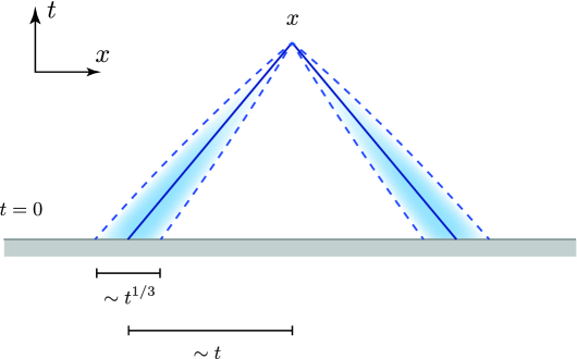
Figure 2: The effect of nonlinear dispersion is to blur the light-cone projections from precise points to spatial intervals, which however remain well separated since their width scales slower with time ($\sim t^{1/3}$ for cubic nonlinearity) than their spatial separation ($\sim t$).

From the explicit relation between time evolved local fields and initial local fields, we can easily derive the long time asymptotics of connected correlation functions. We find that, as a result of the nonlinear dispersion, they vanish at large times for all orders larger than two, i.e. the large time limit is described by a Gaussian state in terms of the bosonisation fields. We will report our results below and present an intuitive explanation, leaving the rigorous derivation for App. A.

Let us start with the two-point function, for which we obtain (87)

$$\lim_{t\to\infty}\mathopen{\hbox{${\bigg{\langle}}$}\kern-2.72221pt\leavevmode\hbox{${\bigg{\langle}}$}}\partial_{x}\hat{\vartheta}(x,t)\partial_{y}\hat{\vartheta}(y,t)\mathclose{\hbox{${\bigg{\rangle}}$}\kern-2.72221pt\leavevmode\hbox{${\bigg{\rangle}}$}} =\frac{1}{2}\int\frac{dk}{2\pi}\,\mathrm{e}^{\mathrm{i}k(x-y)}\left(\tilde{C}_{0}^{(0,0)}(k)+\frac{1}{v^{2}f^{2}(k)}\tilde{C}_{0}^{(1,1)}(k)\right)$$ (45)

Note that the large time two-point correlation function depends significantly on the nonlinearity of the dispersion relation through the function $f(k)$, even if this dependence does not affect its large distance asymptotics, since $f(k)$ is smooth for $k\to 0$ with $f(0)=1$.

For higher order connected correlation functions $n>2$, we find that they decay algebraically with time and the scaling of decaying corrections is controlled by both the large distance decay of initial correlations and the leading power law correction to the linear dispersion relation, i.e. by the low energy limit of

$$\omega(k)-v|k|\sim\lambda|k|^{\gamma}$$ (46)

according to (37). Assuming exponential initial clustering, in which case connected correlation functions have no singularity for real small momenta, we obtain the general scaling law (92)

$$\lim_{t\to\infty}\mathopen{\hbox{${\bigg{\langle}}$}\kern-2.72221pt\leavevmode\hbox{${\bigg{\langle}}$}}\prod_{i=1}^{n}\partial_{x}\hat{\vartheta}(x_{i},t)\mathclose{\hbox{${\bigg{\rangle}}$}\kern-2.72221pt\leavevmode\hbox{${\bigg{\rangle}}$}}\sim\frac{1}{t^{(n-1)/\gamma}}F(\{x_{i}/t^{1/\gamma}\})$$ (47)

where $F(\{s_{i}\})$ has a finite non-zero value when all of its arguments are zero. For algebraic initial clustering, additional multiplicative factors are expected, depending on the low-momentum behaviour of initial correlations. Overall this suggests a certain universality of the scaling of time decaying corrections. Note that in the present case as well as for a Bogoliubov-type dispersion relation, $\gamma=3$ and $\lambda=\frac{1}{2}v\beta$. The same exponent $\gamma=3$ appears in the dispersion relation of typical critical lattice systems, like the critical Ising model, and was proposed to control in a universal way the perturbative corrections to Conformal Field Theory predictions in quantum transport Bernard-Doyon2 . The time decay of transients in out-of-equilibrium problems has been studied extensively both in quench and transport problems long-t-cor_3 ; long-t-cor_2 ; long-t-cor_4 ; long-t-corrections_1 ; bertini_long-t-cor ; Bernard-Doyon , revealing a certain universality of the scaling laws, in agreement with our analysis.

The vanishing of connected correlation functions of order $n>2$ at large times can be seen as a direct consequence of initial clustering and of the uniform time decay of the propagators due to dispersion, using the following simplified and intuitive (though non-rigorous) argument: For sufficient initial clustering, such that the spatial integral of the initial correlation function over the coordinate differences in the whole space is convergent, the large time limit is bounded by the time decaying factors contributed by all but one propagators. In more detail, the relation of the time evolved correlations in terms of initial ones can be written as

$$C(x_{1},...,x_{2};t)=\int_{-\infty}^{+\infty}\prod_{i=1}^{n}dx^{\prime}_{i}\,\prod_{i=1}^{n}\,G(x_{i}-x^{\prime}_{i};t)C_{0}(x^{\prime}_{1},x^{\prime}_{2},...,x^{\prime}_{n})$$ (48)

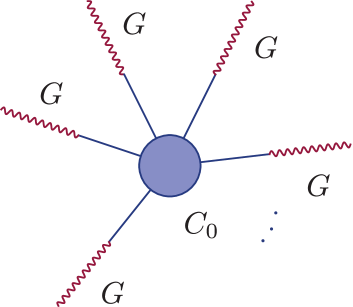
Figure 3: General form of Feynman diagrams for the time evolved connected correlation functions after a quantum quench from an interacting to a free field theory. The central graph (in blue) corresponds to the initial connected correlation function $C_{0}$, while the attached extensions of the external legs (curly red lines) correspond to the propagators $G$ that perform the time evolution.

In the diagrammatic language of quantum field theory, this expression means that time evolution amounts to extending the external legs of initial correlation functions by free propagators of the post-quench Hamiltonian (Fig. 3). Assuming initial clustering such that

$$\int_{-\infty}^{+\infty}\prod_{i=2}^{n}dr_{i}\,\left|C_{0}(0,r{}_{2},...,r_{n})\right|=c_{0}<\infty$$ (49)

and propagator uniformly decaying with time

$$\left|G(x;t)\right|<g(t)\to 0,\text{ as }t\to\infty$$ (50)

with spatial integral bounded as

$$\int_{-\infty}^{+\infty}dr\,G(r;t)<h$$ (51)

the following bound on the time evolved correlations holds

$$\left|C(x_{1},...,x_{n};t)\right| \leq\left|\int_{-\infty}^{+\infty}dx^{\prime}_{1}\,G(x_{1}-x^{\prime}_{1};t)\int_{-\infty}^{+\infty}\prod_{i=2}^{n}d(x^{\prime}_{i}-x^{\prime}_{1})\,\prod_{i=2}^{n}\left|G(x_{i}-x^{\prime}_{i};t)\right|\left|C_{0}(0,x^{\prime}_{2}-x^{\prime}_{1},...,x^{\prime}_{n}-x^{\prime}_{1})\right|\right|$$

$$<c_{0}h\left(g(t)\right)^{n-1}\to 0,\text{ as }t\to\infty\quad(n>2)$$ (52)

In the above we assumed a translationally invariant initial state and dropped the field component indices $\nu_{i}$ to lighten the notation. The condition (49) on the finiteness of the spatial integral of initial correlations should be read as “finite in the thermodynamic limit”, i.e. exhibiting no infrared divergence (ultraviolet divergences are irrelevant in this physical context). The condition (51) of bounded spatial integral of the propagator is generally satisfied as a result of conservation of particle number, which in fact means that $\int_{-\infty}^{+\infty}dr\,G(r;t)=\text{const.}$. Note also that in the above argument, a uniform decay of the propagator is required, i.e. at any time it must be bounded in the whole space by a time decaying function (50), otherwise initial fluctuations may be transported away from their original spatial point but without decaying. We can easily see now the connection between dispersion and time decay of correlations: in systems with conserved particle number, the integral of the propagator over all space is constant in time and therefore dispersive spreading of the propagator is related to decay with time of its maximum value as a function of the spatial coordinate.

Even though the above argument is quite intuitive, it is not rigorous, as the validity of the inequalities relies on mathematical conditions that are not strictly satisfied for the involved functions. For this reason cancellations of oscillatory terms are disregarded by this argument. That is why the argument fails for $n=2$: in this case, the two-point correlations involve terms in which the time dependent oscillatory terms exactly cancel due to the condition of momentum conservation, thus giving a non-vanishing contribution at large times. In contrast, for $n>2$ the momentum conservation condition is not sufficient to ensure the cancellation of oscillatory terms (such cancellations occur only in regions of zero integration measure and do not contribute in the large time limit). A rigorous derivation of the large time asymptotics is given in App. A.

As a last comment, we mention that the monotonicity of the dispersion relation $\omega(k)$ is a non-trivial and relevant assumption, as it affects the form of the Fourier transforms of the derivatives of the propagator. In the context of non-relativistic quantum gases, this assumption breaks down at the bottom of the Luttinger liquid Fermi sea. This is expected to lead to additional time decaying factors that are typically captured by the “mobile impurity” approach of nonlinear Luttinger liquids nonlinear_LL .

V The Effect of Chiral Interaction

We now focus on the opposite limit, in which interaction is present but no dispersion. Using the boson-fermion correspondence, we will see that the bosonic interaction is equivalent to dispersion of the fermionic quasiparticles, thus leading again to a Gaussian GGE but in terms of the fermionised fields this time.

The time evolution is described by the Hamiltonian $\hat{H}_{Lm}+\hat{H}_{int}$ with

$$\hat{H}_{int}=\frac{\alpha}{4\pi}\sum_{\sigma=\pm}\int dx\,\left(\partial_{x}\hat{\varphi}_{\sigma}\right)^{3}$$ (53)

Despite the presence of bosonic interaction, this Hamiltonian can be solved exactly by means of the fermionisation method BF . Indeed, as shown in refermionisation ; qKdV1 , when expressed in terms of the fermionic quasiparticle field defined through the bosonisation formula (19)

$$\hat{\Phi}_{\sigma}^{\dagger}(x)=\hat{F}_{\sigma}\frac{1}{\sqrt{2\pi a}}\mathrm{e}^{2\pi\mathrm{i}\sigma\rho_{0}x}\mathrm{e}^{\mathrm{i}(\sigma\hat{\vartheta}(x)-\hat{\varphi}(x))}$$ (54)

the Hamiltonian $\hat{H}_{int}$ reduces to the non-interacting Hamiltonian of non-relativistic fermions

$$\hat{H}_{int}=\frac{1}{2m^{*}}\sum_{\sigma=\pm}\int dx\,:\left(\partial_{x}\hat{\Phi}_{\sigma}^{\dagger}\right)\left(\partial_{x}\hat{\Phi}_{\sigma}\right):$$ (55)

with effective mass $m^{*}\propto 1/\alpha$.

We will study the time evolution and large time asymptotics of fermionic correlation functions, focusing in particular on density correlations. The method we use is analogous to that of non-relativistic bosons studied in SC_GGE-val and that of the Tonks-Girardeau dynamics of a BEC initial state KCC which in some sense we extend to more general initial states, relying merely on the assumption of clustering of initial fermionic correlations. Indeed as we will see, for the same reasons as in the dispersive case, the large time correlation functions decompose into two contributions, one from each of the two spatial infinities corresponding to the two decoupled chiral fields $\sigma=\pm 1$. We can therefore focus on one of the two chiral components, removing the ballistic coordinate shift of the propagator. The physical problem is then mathematically equivalent to the quench dynamics under the Tonks-Girardeau Hamiltonian, starting from a general initial state.

The Heisenberg equation of motion for the fermion field is

$$\mathrm{i}\partial_{t}\hat{\Phi}_{\pm}(x,t) =\pm\mathrm{i}v\partial_{x}\hat{\Phi}_{\pm}(x,t)-\frac{1}{2m^{*}}\partial^{2}_{x}\hat{\Phi}_{\pm}(x,t)$$ (56)

with solution

$$\hat{\Phi}_{\sigma}(x,t)=\int\mathrm{d}x^{\prime}G_{f}^{\sigma}(x-x^{\prime},t)\hat{\Phi}_{\sigma}(x^{\prime},0)$$ (57)

where

$$G_{f}^{\sigma}(x-x^{\prime},t)=\int\frac{\mathrm{d}k}{2\pi}\,\mathrm{e}^{\mathrm{i}k(x-x^{\prime})+\mathrm{i}k\sigma vt-\mathrm{i}{k^{2}}t/(2m^{*})}=\sqrt{\frac{m^{*}}{2\pi\mathrm{i}t}}\mathrm{e}^{\mathrm{i}m^{*}(x-x^{\prime}+\sigma vt)^{2}/(2t)}$$ (58)

The fermionic two-point correlation function is time independent and automatically described by the fermionic Gaussian GGE, since it is directly related by Fourier transform to the conserved momentum-mode occupation number operators $\hat{n}_{\sigma}(k)=\hat{\Phi}_{\sigma k}^{\dagger}\hat{\Phi}_{\sigma k}$, which play the role of conserved charges of the GGE SC_GGE-val ; KCC . The first non-trivial check of Gaussianity of the steady state comes from the study of density-density correlations and higher order ones. As before we will restrict ourselves to density correlations.

From the bosonisation formula (54) the density field can be easily expressed in terms of the densities of fermionic fields

$$\delta\hat{\rho}(x) \equiv\hat{\Psi}^{\dagger}(x)\hat{\Psi}(x)-\rho_{0}=\frac{1}{\pi}\partial_{x}\hat{\theta}(x)=\sum_{\sigma=\pm}\hat{\Phi}_{\sigma}^{\dagger}(x)\hat{\Phi}_{\sigma}(x)$$ (59)

From the above we find that the time evolution of the density operator is given in terms of the fermion fields by

$$\delta\hat{\rho}(x,t) =\sum_{\sigma=\pm}\int\mathrm{d}s\mathrm{d}s^{\prime}\,G_{f}^{\sigma*}(x-s,t)G_{f}^{\sigma}(x-s^{\prime},t)\;\hat{\Phi}_{\sigma}^{\dagger}(s,0)\hat{\Phi}_{\sigma}(s^{\prime},0)$$ (60)

This formula for the general solution of the equations of motion has been derived in equivalent form in qKdV1 ; qKdV2 . We therefore find that the $n$-point density correlation function is given in terms of initial $2n$-point fermionic correlation functions

$$\left\langle\prod_{i=1}^{n}\delta\hat{\rho}(x_{i},t)\right\rangle =\sum_{\sigma_{i}=\pm}\int\mathrm{d}s_{i}\mathrm{d}s_{i}^{\prime}\,\prod_{i=1}^{n}G_{f}^{\sigma_{i}*}(x_{i}-s_{i},t)G_{f}^{\sigma_{i}}(x_{i}-s_{i}^{\prime},t)\;\left\langle\prod_{i=1}^{n}\hat{\Phi}_{\sigma_{i}}^{\dagger}(s_{i},0)\hat{\Phi}_{\sigma_{i}}(s^{\prime}_{i},0)\right\rangle$$ (61)

For the connected correlation functions of the density, using the multi-linearity of connected correlations, we find

$$\mathopen{\hbox{${\bigg{\langle}}$}\kern-2.72221pt\leavevmode\hbox{${\bigg{\langle}}$}}\prod_{i=1}^{n}\delta\hat{\rho}(x_{i},t)\mathclose{\hbox{${\bigg{\rangle}}$}\kern-2.72221pt\leavevmode\hbox{${\bigg{\rangle}}$}}=\sum_{\sigma_{i},\sigma^{\prime}_{i}=\pm}\int\mathrm{d}s_{i}\mathrm{d}s_{i}^{\prime}\,\prod_{i=1}^{n}G_{f}^{\sigma_{i}*}(x_{i}-s_{i},t)G_{f}^{\sigma^{\prime}_{i}}(x_{i}-s_{i}^{\prime},t)\;C_{0f}^{\{\sigma_{i},\sigma^{\prime}_{i}\}}\left(\{(s_{i},s_{i}^{\prime})\}\right)$$

$$=\sum_{\sigma_{i},\sigma^{\prime}_{i}=\pm}\int\prod_{i=1}^{n}\frac{dk_{i}dk^{\prime}_{i}}{(2\pi)^{2}}\,\mathrm{e}^{\mathrm{i}\sum_{i}\left[-(k_{i}-k^{\prime}_{i})x_{i}-\mathrm{i}\left(k_{i}\sigma_{i}-k^{\prime}_{i}\sigma^{\prime}_{i}\right)vt+\mathrm{i}(k_{i}^{2}-\left.k^{\prime}_{i}\right.^{2})t/(2m^{*})\right]}\;\delta({\textstyle\sum_{i}k_{i}-\sum_{i}k^{\prime}_{i}})\tilde{C}_{0f}^{\{\sigma_{i},\sigma^{\prime}_{i}\}}\left(\{(k_{i},k^{\prime}_{i})\}\right)$$ (62)

where

$$C_{0f}^{\{\sigma_{i},\sigma^{\prime}_{i}\}}\left(\{(s_{i},s_{i}^{\prime})\}\right)=\mathopen{\hbox{${\bigg{\langle}}$}\kern-2.72221pt\leavevmode\hbox{${\bigg{\langle}}$}}\prod_{i=1}^{n}\hat{\Phi}_{\sigma_{i}}^{\dagger}(s_{i},0)\hat{\Phi}_{\sigma_{i}}(s^{\prime}_{i},0)\mathclose{\hbox{${\bigg{\rangle}}$}\kern-2.72221pt\leavevmode\hbox{${\bigg{\rangle}}$}}$$ (63)

are $2n$-point initial fermionic connected correlation functions.

At this point we should analyse the condition of cluster decomposition property of initial fermionic correlation functions, since there are some obvious differences with the previous case. This condition is non-trivial because, unlike the boson field $\hat{\Psi}^{\dagger}(x)$, the fermion field $\hat{\Phi}_{\sigma}^{\dagger}(x)$ is essentially non-local. Indeed from the bosonisation formula (54) which defines the fermion field in terms of the bosonisation fields, by expressing the exponent in terms of chiral field derivatives, which are local fields, we find

$$\hat{\Phi}_{\sigma}^{\dagger}(x)\sim\mathrm{e}^{\mathrm{i}\pi\int_{-\infty}^{x}\hat{\rho}_{\sigma}(x^{\prime})\mathrm{d}x^{\prime}}$$ (64)

where $\hat{\rho}_{\sigma}(x)=\partial_{x}\hat{\varphi}_{\sigma}(x)/\pi$ corresponds to densities of chiral fields. The above relation is essentially a Jordan-Wigner type of transformation nonlinear_LL , which is manifestly non-local. Despite this fact, it can be shown that at least a weak version of the cluster property is still valid for the fermionic correlations. While we cannot provide a general proof that the strong version of cluster property is also valid, i.e. that clustering of bosonic correlations would also imply clustering of fermionic correlations, nevertheless by studying special types of fermionic correlation functions we find evidence that this may be true. In fact even if bosonic correlations exhibit mild algebraic clustering, fermionic correlations can exhibit exponential clustering, as is the case for at least one type of state studied in the literature KCC . A detailed analysis of fermionic clustering property is given in App. B.

Assuming that the clustering property holds for the fermionic correlations, we can follow the same arguments as in the previous dispersive case. Since the propagator (58) decays with time uniformly in the whole space, assuming sufficiently fast decaying initial correlations, the connected correlations decay with time. We also find that the leading contributions to the large time limit come from the left and right spatial infinities, since the propagators spread slower than the ballistic separation of the left and right lightcone projections. This can be seen from (62): it is only the terms with all $\sigma_{i}=\sigma^{\prime}_{i}$ that determine the slowest time decay, since all other terms come with extra factors of $1/t$. Therefore

$$\lim_{t\to\infty}\mathopen{\hbox{${\bigg{\langle}}$}\kern-2.72221pt\leavevmode\hbox{${\bigg{\langle}}$}}\prod_{i=1}^{n}\delta\hat{\rho}(x_{i},t)\mathclose{\hbox{${\bigg{\rangle}}$}\kern-2.72221pt\leavevmode\hbox{${\bigg{\rangle}}$}} =\lim_{t\to\infty}\sum_{\sigma=\pm}\int\prod_{i=1}^{n}\frac{dk_{i}dk^{\prime}_{i}}{(2\pi)^{2}}\,\mathrm{e}^{-\mathrm{i}\sum_{i}(k_{i}-k^{\prime}_{i})x_{i}+\mathrm{i}\sum_{i}(k_{i}^{2}-\left.k^{\prime}_{i}\right.^{2})t/(2m^{*})}\;\delta({\textstyle\sum_{i}k_{i}-\sum_{i}k^{\prime}_{i}})\tilde{C}_{0f}^{\sigma}\left(\{(k_{i},k^{\prime}_{i})\}\right)$$ (65)

By re-scaling the integration variables, the above formula suggests as a maximum bound of the time decay the following scaling relation

$$\lim_{t\to\infty}\mathopen{\hbox{${\bigg{\langle}}$}\kern-2.72221pt\leavevmode\hbox{${\bigg{\langle}}$}}\prod_{i=1}^{n}\delta\hat{\rho}(x_{i},t)\mathclose{\hbox{${\bigg{\rangle}}$}\kern-2.72221pt\leavevmode\hbox{${\bigg{\rangle}}$}}<t^{-(2n-1)/2}F_{f}(\{x_{i}^{2}/t\})$$ (66)

However the time decaying factor in this relation is overestimated, since the antisymmetry of the initial fermionic correlation functions means that there may be extra factors of $k_{i},k^{\prime}_{i}$ in the integrand that downgrade it further.

To summarise this section, we have shown that, provided that initial correlations satisfy sufficient clustering (in terms of the fermion field this time), connected correlation functions of the density of order $n>1$ decay with time, as a consequence of the time decay of the propagators. This means that the large time limit of density correlations is given by an ensemble that is Gaussian in terms of the fermionic quasiparticle field.

VI Semiclassical Analysis of the Quantum KdV Equation

We now consider the time evolution under the quantum KdV Hamiltonian. Integrability of the quantum KdV and related modified equations has been studied due to their connection with Conformal Field Theories BLZ . The construction of commuting local conserved charges has been studied in qKdV_charges and the Algebraic Bethe Ansatz formulation has been studied in KdV+ABA . Unlike the previous essentially free models, the exact general solution of the Heisenberg equations of motion is not known, however some hints about the nature of the dynamics can be drawn from the semiclassical approximation qKdV-LL ; GP-solitons . The latter ignores the effects of quantum fluctuations on local fields, but is expected to give qualitatively correct results. Under this approximation, the time evolution of a local perturbation of the density is described by the classical KdV equation, which is known to exhibit solitary wave solutions, i.e. ballistically moving localised and shape-preserving waves. Their existence, perhaps the most characteristic feature of integrability, is due to a cancellation of the effects of dispersion and non-linearity (interaction). Moreover it is known that the long time asymptotics of the solution for a general initial condition consists always of a set of solitary waves with different velocities and a continuum of decaying dispersive waves math:KdV_asympt . In particular point-like initial fluctuations always decompose asymptotically to exactly one solitary wave for each of the two chiral modes, together with a dispersive component. Below we review the semiclassical analysis as well as general results for the long time asymptotics of the classical KdV in more detail.

We first derive the equations of motion corresponding to the quantum KdV Hamiltonian

$$\hat{H}_{KdV}=\frac{1}{4\pi}\sum_{\sigma=\pm}\int dx\,\left[\alpha\left(\partial_{x}\hat{\varphi}_{\sigma}\right)^{3}+\beta\left(\partial_{x}^{2}\hat{\varphi}_{\sigma}\right)^{2}\right]$$ (67)

As in the classical KdV equation, the parameters $\alpha$ and $\beta$ can be absorbed by a suitable redefinition of space and time variables. We can therefore write

$$\sigma\partial_{t}\hat{\varphi}_{\sigma}=\frac{3}{2}:\left(\partial_{x}\hat{\varphi}_{\sigma}\right)^{2}:-\partial_{x}^{3}\hat{\varphi}_{\sigma}$$ (68)

Since the two chiral components of the field evolve independently, we can focus on one of them, say the right moving one, $\sigma=+$. The solution for the other chiral component can be found by a simple space reflection transformation. The equation for the local derivative field $\hat{u}=\frac{1}{2}\partial_{x}\hat{\varphi}_{+}$ is

$$\partial_{t}\hat{u}=3:\left[\left(\partial_{x}\hat{u}\right)\hat{u}+\hat{u}\left(\partial_{x}\hat{u}\right)\right]:-\partial_{x}^{3}\hat{u}$$ (69)

We are interested in the localisation properties of the operator-valued field solution of the above equation in the long time limit. In absence of exact results for the general solution, we restrict ourselves to a partial check that can be performed using the semiclassical approximation. More specifically we will consider the dynamical response of the system to an arbitrary localised initial fluctuation, i.e. a local quantum quench. This problem has been previously studied in GP-solitons considering as initial state a soliton configuration corresponding to different values of the parameters of the Hamiltonian. It was shown that this pre-quench soliton splits into two stable localised wavepackets moving to opposite directions. This should be compared with the previously studied cases: in the presence of either dispersion or interaction the dynamics for such a local quench would result in spreading of the initially localised fluctuation and decay of its amplitude with time.

The semiclassical approximation corresponds to considering the expectation value of the above equation in some state of the bosonised Hilbert space and ignoring the effects of local quantum fluctuations, i.e. approximating the expectation value of the product of operators in the above equation by the product of their expectation values. Setting $u(x,t)=\langle\hat{u}(x,t)\rangle$ and applying the semiclassical approximation in the above equation for the right moving chiral mode, we end up with the standard form of the classical KdV equation

$$\partial_{t}u(x,t)=6u(x,t)\partial_{x}u(x,t)-\partial_{x}^{3}u(x,t)$$ (70)

As is well-known, this classical equation admits solitary wave solutions, as well as multi-soliton solutions and dispersive wave solutions. Its general solution for an arbitrary initial condition is given by the inverse scattering transform. In combination with the nonlinear steepest descent method, it has be shown that at long times any initially localised field profile decomposes to a superposition of one or more solitons moving at different velocities to the same direction and a decaying in time dispersive part moving to the opposite direction math:KdV_asympt . A short overview of the properties of the classical KdV equation is given in App. C. The above general result shows that, at least in the regime of validity of the semiclassical approximation, localised field fluctuations evolve so that they always form ballistically moving localised excitations. The effect of quantum fluctuations may however affect the stability of solitons, ultimately leading to complete decay of these excitations. Below we analyse the effects of potentially stable quantum solitons on equilibration.

VII Quantum Solitary Waves and Equilibration

We showed that evolution under the standard Luttinger model preserves the memory of initial correlations up to infinite times. We will now show that this effect can be interpreted as a consequence of the ballistic and localised character of excitations in the standard Luttinger model. Motivated by the semiclassical analysis of the quantum KdV equation, we then conclude that whenever solitary waves remain stable at the quantum level, equilibration exhibits the same memory preservation effect.

As explained earlier, using the boson-fermion correspondence

$$\hat{\Phi}_{\sigma}^{\dagger}(x)=\hat{F}_{\sigma}\frac{1}{\sqrt{2\pi a}}\mathrm{e}^{2\pi\mathrm{i}\sigma\rho_{0}x}\mathrm{e}^{\mathrm{i}(\sigma\hat{\vartheta}(x)-\hat{\varphi}(x))}$$ (71)

the Luttinger model can be equivalently written as a system of free fermions with linear dispersion, i.e. free massless Majorana fermions in the language of relativistic field theory

$$\hat{H}_{Lm} =-\mathrm{i}v\sum_{\sigma=\pm}\sigma\int dx\,:\hat{\Phi}_{\sigma}^{\dagger}(x)\partial_{x}\hat{\Phi}_{\sigma}(x):$$ (72)

The operators $\hat{\Phi}_{\sigma}^{\dagger}(x)$ can be recognised as soliton creation operators Mandelstam , since their commutation relations with the bosonisation field $\hat{\varphi}(x)$ are

$$[\hat{\varphi}_{\sigma}(x),\hat{\Phi}_{\sigma}^{\dagger}(x^{\prime})] =\pi\Theta(x-x^{\prime})\hat{\Phi}_{\sigma}^{\dagger}(x^{\prime})$$ (73)

where $\Theta(x)$ is the step function. This means that $\hat{\Phi}_{\sigma}^{\dagger}(x)$ creates a static soliton state out of the vacuum. The equations of motion for the soliton operator under $\hat{H}_{Lm}$ are

$$\partial_{t}\hat{\Phi}_{\sigma}^{\dagger}(x,t) =\sigma v\partial_{x}\hat{\Phi}_{\sigma}^{\dagger}(x,t)$$ (74)

whose general solution in terms of the initial conditions is

$$\hat{\Phi}_{\sigma}^{\dagger}(x,t) =\hat{\Phi}_{\sigma}^{\dagger}(x+\sigma vt,0)$$ (75)

We see that the soliton operators evolve purely ballistically. This feature is expected to be valid in any other system in which there exist local field operators whose evolution satisfies the wave equation, like for example the massless Thirring model.

Note the distinction we use between the terms “soliton” and “solitary wave”: the former is used to describe static field configurations interpolating between different asymptotic vacua, while the latter describe dynamical fields, i.e. operatorial solutions of the Heisenberg equation of motion, that correspond to ballistically moving localised fields. Static solitons may be stable or unstable in which case they decompose to other excitations, depending on the Hamiltonian that governs their time evolution. Solitary waves may have no connection with static solitons or may correspond to clusters of solitons. In the present case, where the conservation of boson particle number constrains us to the Hilbert space sector with zero overall solitons, such excitations appear in the initial state only in pairs of soliton creation and annihilation operators.

From the above relation we can derive the large time limit of any fermionic correlation function in terms of initial ones, assuming that the initial state satisfies translation invariance and cluster property in terms of the fermions

$$\lim_{t\to\infty}\mathopen{\hbox{${\bigg{\langle}}$}\kern-2.72221pt\leavevmode\hbox{${\bigg{\langle}}$}}\prod_{i=1}^{n}\hat{\Phi}_{\sigma_{i}}^{\dagger}(x_{i},t)\hat{\Phi}_{\sigma_{i}}(y_{i},t)\mathclose{\hbox{${\bigg{\rangle}}$}\kern-2.72221pt\leavevmode\hbox{${\bigg{\rangle}}$}}=\sum_{\sigma=\pm}\mathopen{\hbox{${\bigg{\langle}}$}\kern-2.72221pt\leavevmode\hbox{${\bigg{\langle}}$}}\prod_{i=1}^{n}\hat{\Phi}_{\sigma}^{\dagger}(x_{i})\hat{\Phi}_{\sigma}(y_{i})\mathclose{\hbox{${\bigg{\rangle}}$}\kern-2.72221pt\leavevmode\hbox{${\bigg{\rangle}}$}}$$ (76)

Let us now consider the general case of an interacting evolution equation, like the quantum KdV. The time evolution of the field in the Heisenberg picture is $\hat{\phi}(x,t)=\mathrm{e}^{\mathrm{i}\hat{H}t}\hat{\phi}(x)e^{-i\hat{H}t}$ where $\hat{\phi}(x)=\hat{\phi}(x,0)$ is the initial field configuration. Using the general Baker-Campbell-Hausdorff formula, we can formally express $\hat{\phi}(x,t)$ as an expansion in a basis of initial, not necessarily local, fields

$$\hat{\phi}(x,t)=\sum_{\alpha}\int_{-\infty}^{+\infty}dx^{\prime}\,G_{\alpha}(x-x^{\prime};t)\hat{\Phi}_{\alpha}(x^{\prime})$$ (77)

This formal expansion represents the propagation of field fluctuations from the initial state up to time $t$. The basis $\{\hat{\Phi}_{\alpha}\}$ is in general infinite and includes derivatives of $\phi$ of any order, as well as composite operators. Clearly the fields $\hat{\Phi}_{\alpha}$ are not limited to local fields. Even though for a continuous Hamiltonian involving only contact interactions, the Baker-Campbell-Hausdorff formula would produce commutators that are seemingly local (derivatives of the Dirac $\delta$-function of arbitrary high order), such fields are ill-defined and require normal-ordering or point-splitting that essentially means that they are non-local. This can be clearly seen in lattice systems where the general term corresponds to a composite operator of arbitrarily large length of spatial support. In the case of a Hamiltonian quadratic in $\hat{\phi}$ and its canonically conjugate field $\hat{\pi}=\partial_{t}\hat{\phi}$ satisfying the canonical commutation relation $[\hat{\phi}(x),\hat{\pi}(x^{\prime})]=i\delta(x-x^{\prime})$, the algebra of these operators closes and we obtain a linear evolution

$$\hat{\phi}(x,t)=\int_{-\infty}^{+\infty}dx^{\prime}\,\left(\dot{G}(x-x^{\prime};t)\hat{\phi}(x^{\prime})+G(x-x^{\prime};t)\hat{\pi}(x^{\prime})\right)$$ (78)

Dispersive modes would be associated with time decaying propagators $G_{\alpha}(x;t)$. Instead solitary wave solutions of the Heisenberg equations of motion are defined as localised operator solutions that evolve ballistically i.e. of the form

$$\hat{\phi}(x,t)=\hat{\Phi}_{s}(x-v_{s}t-x_{0})$$ (79)

where $x_{0}$ is a free parameter, the initial position of the solitary wave, and $v_{s}$ is its velocity. Equivalently, such localised fields satisfy the dynamical condition

$$\mathrm{e}^{\mathrm{i}Ht}\hat{\Phi}_{s}(x)\mathrm{e}^{-\mathrm{i}Ht}=\hat{\Phi}_{s}(x-v_{s}t)=\mathrm{e}^{-\mathrm{i}Pv_{s}t}\hat{\Phi}_{s}(x)\mathrm{e}^{\mathrm{i}Pv_{s}t}$$ (80)

where $\hat{P}$ is the momentum operator, generator of spatial translations. The above equation suggests that the operators $\hat{\Phi}_{s}(x),\hat{H}$ and $\hat{P}$ form a closed subalgebra. The localisation condition can be expressed as exponential decay with the distance of the norm of the commutator between the solitary wave operator and the fundamental local field

$$\left\|\left[\hat{\Phi}_{s}(x),\hat{\phi}(y)\right]\right\|<\text{const.}\,\mathrm{e}^{-\lambda_{s}|x-y|}$$ (81)

We will call such solutions “quantum solitary waves”. The existence of such solutions depends on whether quantum corrections preserve the localisation features of the classical solitary waves or not, and in general it cannot be excluded from first principles.

Motivated by the semiclassical results for the KdV equation, let us now consider an analogous large time asymptotic expansion in the quantum case, i.e. that any initial field configuration $\hat{\phi}_{0}(x)$ evolves so that it eventually splits into a number of quantum solitary waves $\hat{\Phi}_{s}$ and a time decaying dispersive component $\hat{R}$. In this case we would write a formal expansion

$$\hat{\phi}(x,t)\sim\sum_{s}\hat{\Phi}_{s}(x-x_{0s}-v_{s}t)+\hat{R}(t),\ \text{for }t\to\infty$$ (82)

where the residual component $\hat{R}(t)$ has extensive spatial support, but its projection onto a local basis of field operators decays uniformly with time. In analogy to the classical case we may expect that the above sum consists of a single solitary wave only, since the initial field configuration $\hat{\phi}_{0}(x)$ is a point-like field. However we do not need to restrict ourselves with this expectation.

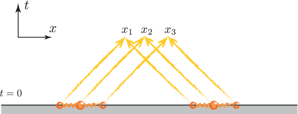
Figure 4: Equilibration in the presence of quantum solitary waves in 1D hydrodynamic systems: Due to their localised nature and ballistic dynamics, large time correlations between a set of points are equal to the initial solitary wave field correlations at their light-cone projections. Due to clustering of initial correlations, the large time correlations are decomposed into a sum of two components originating from the two spatial infinities.

By now it should be obvious what the consequences of this scenario would be for our quench problem. Let us focus on the long time asymptotics of connected correlation functions of the local field $\hat{\phi}(x,t)$. Using the above formula and applying it to the time inverted evolution in order to trace back to the initial fields from which the large time field $\hat{\phi}(x,t)$ originates, we obtain

$$\lim_{t\to\infty}\left\langle\prod_{i}\hat{\phi}(x_{i},t)\right\rangle=\lim_{t\to\infty}\left\langle\prod_{i}\sum_{s}\hat{\Phi}_{s}(x_{i}-x_{0s}-v_{s}t)+\hat{R}(t)\right\rangle$$ (83)

We can omit the time decaying dispersive part, except for the two point functions where it does contribute, as in the non-interacting case. Since the solitary wave operators are spatially localised and moving away from each other due to their different velocities, from the cluster property of the initial state the above correlation function splits into a sum of clusters of same type solitary waves. Lastly using the translational invariance of the initial state we can remove the coordinate shifts $-x_{0s}-v_{s}t$. We therefore conclude that

$$\lim_{t\to\infty}\left\langle\prod_{i}\hat{\phi}(x_{i},t)\right\rangle =\sum_{s}\left\langle\prod_{i}\hat{\Phi}_{s}(x_{i})\right\rangle_{0}$$ (84)

which means that initial correlations of solitary wave operators of all orders survive up to infinite time (Fig. 4). Note that the key features of the definition of quantum solitary waves that are important in the above arguments are that they are localised fields, so that their correlations satisfy the cluster property, and that they are preserved by time evolution, in particular that the norm of the time-evolved operators does not reduce with time, as that of the dispersive components.

VIII Discussion of results

Experimental relevance

Experimental realisation of quench protocols that are described by continuous quantum field theories has been achieved in the framework of 1D split atomic quasi-condensates, which has recently led to the celebrated first observation of a GGE exp:GGE . The theoretical description of such cold-atom experiments, assuming point-like interactions, is given by the integrable Lieb-Liniger model. On the other hand, their low-energy effective description in terms of the atomic wavefunction’s density and phase fields is given by the sine-Gordon model and, in the gapless phase, the Luttinger model exp:sG3 ; exp:sG2 . More specifically it has been argued that the experimental system can be prepared in a state that resembles the ground state of the sine-Gordon model for arbitrary interaction exp:sine-Gordon . Basic features of the general sine-Gordon ground state, like the non-Gaussianity of correlation functions and the presence of massive excitations and static solitons, have been observed experimentally. On the other hand, the evolution Hamiltonian is typically chosen to lie in the gapless regime, which is described at low-energies by the standard Luttinger model exp:lightcone1 ; exp:lightcone2 ; exp:LL . In particular the light-cone form of dynamics as predicted by the Luttinger model has been observed in exp:lightcone1 .

Both the sine-Gordon model and the Luttinger model are only low-energy effective descriptions of the actual system, which may not be expected to provide exact descriptions of quantum quenches, due to the fact that instantaneous quenches typically create excitations of arbitrarily high-energies. One way to suppress the creation of high-energy excitations so as to remain in the regime of validity of the low-energy approximation, is to perform the quench over a finite time interval, which is perhaps a more realistic experimental protocol. In fact the observation of a light-cone effect, despite the non-relativistic nature of the system, may be a sign that the presence of high-energy excitations in the initial state is suppressed.

On the contrary, in order to take into account the presence of high-energy excitations, it is necessary to go beyond the standard Luttinger model description and include the effects of non-linear dispersion and interactions on the dynamics, which are captured by quantum hydrodynamic models, like the quantum KdV model studied here. Therefore the quantum analogue of the problem Zabusky and Kruskal considered 50 years ago ZK can now be studied efficiently in cold atom experiments.

Our analysis shows that in the standard Luttinger model, due to the purely ballistic nature of dynamics, dephasing is prevented and equilibration is characterised by preservation of the memory of initial non-Gaussian correlations. In the presence of dispersion or self-interaction of the bosonised fields, this memory effect breaks down and the steady state is a Gaussian GGE in terms of the bosonisation or fermionisation fields respectively. Dispersion of the bosonised fields is a consequence of a non-local interaction between the original bosons or next-to-leading order contributions of the kinetic energy in the hydrodynamic equations. On the other hand, interaction between the bosonised fields corresponds to non-linear dispersion of the original boson fields. The combination of dispersion and interaction gives rise to a new possibility, the formation of solitary waves, the stability of which under the effect of quantum fluctuations remains an open problem. In the presence of such ballistic localised excitations the previous memory preservation effect is restored. In this context, more specifically in the Lieb-Liniger description of the experimental system, solitons have been proposed to correspond to Lieb’s second type of excitations which describe hole excitations. In exp:GGE instead a Bogoliubov dispersion relation is used for the description of the post-quench excitations. This type of dispersion is associated with Lieb’s first type of fundamental excitations that describe phononic excitations. Assuming that excitations of the second type are suppressed in the initial state, our analysis suggests that, as a result of the dispersion of the phonons, the steady state is Gaussian in terms of the density and phase fields.

It is worth mentioning that, in the same way that integrability, as an approximation of real physical systems, manifests itself on their dynamics as pre-thermalisation described by a GGE-type equilibration before thermalisation eventually takes place, quantum hydrodynamics may also be expected to describe the early stages of quench dynamics. In particular, considered as an approximation of other integrable models, quantum hydrodynamical equilibration would correspond to a “pre-equilibration” stage, before equilibration to some version of the GGE takes place. This scenario relies however on the assumption of a clear separation between the power-law exponents characterising the temporal decay of corrections at each of these stages. In fact we have already seen that the low-momentum scaling of the dispersion relation of different types of excitations determines the large time decay of transients before equilibration is finally reached.

Comparison with the GGE and Quench Action method

Let us now clarify the relation of our arguments and approach with two main concepts in the field of out-of-equilibrium quantum physics in general integrable models: the GGE and the Quench Action method. We have argued that the presence of ballistically moving localised excitations, like stable quantum solitons, is associated with preservation of the memory of all their initial correlations at all times. In such systems, like in the standard Luttinger model discussed here, mere knowledge of the initial density of excitations is not sufficient for the complete description of the long time steady state. Nevertheless, even though solitary waves are one of the principal features of classical integrability, the existence of such excitations in quantum integrable systems remains largely unexplored. Adopting the above point of view, we are led to the conclusion that in principle integrable dynamics do not necessarily identify with the memory loss of conventional equilibration and the economy that characterises typical statistical ensembles. Instead, the decisive factor regarding the information content of the steady state appears to be the locality properties of the excitations, which is only indirectly constrained by integrability.

While the GGE has been implicitly associated with extensive memory loss, since the number of local charges in a typical integrable model increases only linearly with the system size, in fact its precise definition is less restricting than that: it is always possible that there exist additional local or quasi-local charges whose number increases faster than linearly with the system size and which would capture all necessary information. In a non-interacting system, like the standard Luttinger model, such charges would have to be non-quadratic in the fields so that the large time steady state is non-Gaussian in terms of them. In this scenario the GGE would be still valid, even though it would be qualitatively different from its conventional form and no longer economic: the number of required charges would not increase simply linearly with the system size as typically in integrable models but rather exponentially, like the number of clusters between different points, a feature characteristic of super-integrability or non-Abelian integrability non-abelian , rather than mere integrability. Moreover, the question of existence of unknown extra charges perhaps makes this problem of academic rather than practical interest.

In general, although from a fundamental perspective it is important to understand if the set of local charges is indeed sufficient for the complete description of the steady state in a general quantum quench problem, from a practical point of view it is more important to develop methods to extract partial information about the steady state (a particular physical observable) from partial information about the initial state (a set of initial observables). This is even more essential in systems where the local charges are not explicitly known or, even if they are, they are ill-defined, as is typically the case in continuous systems. On the other hand, while explicit knowledge of the expansion of the initial state in terms of post-quench eigenstates provides all information needed for the calculation of, in principle, any local observable, in practice the derivation of such expansions can be achieved inevitably only for special types of initial states, like those involving only pairs of oppositely moving excitations BEC1 ; BEC2 ; KCC ; Neel ; atr_LL . The method advocated here circumvents completely both problems of finding the expansion of the initial state and of determining the set of suitable charges of the GGE and deriving its predictions. Instead, our approach is to track the origin of the information that is required for the derivation of large time observables from initial ones, by focusing on the long time asymptotics of solutions of the Heisenberg equations of motion.

Another analytical method for the solution of quantum quench problems in Bethe Ansatz solvable models, which is largely inspired by statistical physics concepts, is the so-called Quench Action or representative state method QA ; QA2 . In this approach the initial state is described in the thermodynamic limit by a representative state and nearby excitations DNPC . Under the assumption of dephasing during the time evolution, the effect of such excitations decays with time, so that in the large time limit local observables are expected to be completely described by the representative state only. According to this approach the large time steady state for a non-interacting model is predicted to be Gaussian and only information about the density of momentum excitations is expected to survive at large times, as long as we restrict ourselves to local observables. We have demonstrated that this is not true for systems with non-interacting dynamics characterised by linear dispersion, where essentially all information about non-Gaussian initial correlations is transferred intact up to infinite times. The reason is quite simple: one of the conditions of the quench action method is that the evolution induces dephasing that wipes out all information about separate clusters of initial excitations, which is obviously not valid here. More specifically, even if it is true that the initial state can be completely described by a representative state and the set of adjacent excitations, in the absence of dephasing all such excitations remain present in the steady state and therefore the representative state alone does not provide a complete description.

In general, the physical conditions on the dynamics that would guarantee sufficient dephasing in order for the quench action method to be applicable remain to be specified. While the linear dispersion considered above is an idealised and rather unrealistic case, as we have argued the same memory effect is expected to be present in systems exhibiting stable solitons, a genuine feature of classical integrability albeit elusive in the framework of the Bethe Ansatz solution for quantum integrable models. Therefore it remains an interesting open question to test if sufficient dephasing takes place in general, especially when the initial state does not simply consist of opposite momentum pair excitations BEC1 ; BEC2 ; KCC ; Neel ; atr_LL . Such states are special and analogous to Gaussian states in non-interacting systems, in the sense that they are fully determined by their density of momentum excitations, for which reason they are not so suitable for the study of memory loss.

IX Conclusions & Outlook

We have studied quench dynamics and equilibration in quantum hydrodynamic systems. Equilibration in such systems presents special interest since, due to the gaplessness of the evolution Hamiltonian, the stationary phase argument which is the typical explanation of dephasing in quantum systems is not directly applicable. Moreover, as we have shown, the low-energy description of such systems as given by the standard Luttinger model exhibits purely ballistic dynamics which prevents dephasing so that equilibration preserves the memory of non-Gaussian initial correlations. However, while the gaplessness of the energy spectrum appears to be a necessary condition for this memory effect, it is not a sufficient one. What we have shown in the present work is that this effect is actually a consequence of a very delicate property of the Luttinger model, its linear dispersion relation. In fact, the presence of either dispersion or chiral interactions, which are irrelevant at equilibrium, breaks down this effect and induces dephasing so that the steady state is given by a Gaussian GGE in terms of the bosonisation or fermionisation fields respectively. In the case of simultaneous presence of both dispersion and chiral interactions, the interplay between these two effects and their role on equilibration remains an open problem, since the potential formation of dynamically stable quantum solitons would restore the ballistic localised character of dynamics and the memory preservation effect. Following the connection between the nature of equilibration and transport properties introduced in Eisert16 , we have identified quantum solitons as carriers of information of initial correlations in quantum quenches, opening a new perspective to the ongoing research on the stability of soliton excitations in 1D quantum systems q_hydrodyn1 ; QH0 ; QH1 ; QH2 ; QH3 ; QH4 .

Although we have focused on aspects of quench dynamics and equilibration in 1D quantum hydrodynamics, our analysis has consequences on several physical problems in the broader context of quantum out-of-equilibrium physics. First of all, our analysis of the effects of dispersion provides a number of conclusions about the application of Luttinger liquid theory to quantum quenches Cazalilla ; s-jstat3 . It is clear that the standard Luttinger model does not lead to Gaussian relaxation in terms of the bosonised fields, since a non-Gaussian initial state would remain such for all times due to the linear dispersion relation. (It is still possible however that an out-of-equilibrium version of the “Luttinger liquid conjecture” for the relation between exponents of correlation functions, analogous to that at equilibrium LL_conj , may still hold out of equilibrium.) In order to study quench dynamics and equilibration it is therefore necessary to go beyond the standard Luttinger model with linear dispersion and take into account e.g. dispersion effects which are the result of a non-local interaction or next-to-leading order contributions of the kinetic energy Cazalilla . In this case, the steady state correlations depend significantly on the nonlinearity of the dispersion relation, as shown in (45), even though the latter does not affect their large distance asymptotics. These remarks may explain the minor discrepancies between numerics and Luttinger liquid predictions in spin chains observed in CCE .

While we focused our analysis on the quantum KdV equation, which provides a general low-energy effective description of the one-dimensional interacting Bose gas, the latter can be faithfully described also by the Lieb-Liniger model, an integrable model of non-relativistic bosons with contact interactions that can be solved exactly by means of the Bethe Ansatz. In the case of repulsive interaction, evolution under the Lieb-Liniger Hamiltonian is expected to lead to dispersion of the KdV solitons, at least on the basis of semiclassical calculations qKdV-LL . It is worth mentioning that the soliton dispersion relation is different from that of phonons and would lead to a slower dispersion as $t^{-5/2}$. It can be therefore expected that it is exactly the soliton excitations that govern the large time scaling of the corrections to equilibration. In the attractive case, on the other hand, such localised solutions are expected to be more stable and may be linked to many particle bound states. A challenging question is to study the soliton stability in the attractive Lieb-Liniger model and their effect on equilibration after a quench starting from a general initial state.

Our analysis of the dispersionless interacting KdV applies equally well to general quantum quenches to the Tonks-Girardeau limit of quantum gases, since in this case the dynamics is described essentially by the same free fermion Hamiltonian. We have shown that, at least under the assumption of clustering of fermionic correlations in the initial state, the large time density correlations are Gaussian, thus generalising results of KCC for the BEC state. However, as we explained, the condition of initial clustering of fermionic correlations is non-trivial, due to the non-local nature of the Jordan-Wigner transformation. We have shown that clustering is valid for composite fermionic operators of even number and we have given some arguments that the exponential clustering observed for the BEC state KCC is expected to be more generally valid.

Evidence for the existence of dynamically stable quantum solitons comes mainly from continuous rather than lattice systems. Indeed, in the most prominent examples of integrable spin chains, like the XXZ model, dispersion seems to always dominate, so that initially prepared static solitons spread and appear to decay with time when they are let to evolve spin-chain_solitons . It is an interesting question if this type of behaviour holds generally as a consequence of some more fundamental property. For example, a general feature of the dynamics of spin chains with short (finite) range interactions is the Lieb-Robinson bound LR ; Lieb-Robinson ; LR_BHV , i.e. the existence of a maximum velocity of signal propagation. This bound constrains the dynamics and the excitation spectrum, so that it may obstruct the emergence of stable solitons. Long-range lattice systems instead, similarly to continuous non-relativistic systems, do not exhibit such constraints on their dynamics.

Our analysis may also be relevant to the problem of quantum transport in integrable models, as in the case of quenches starting from inhomogeneous initial states. In this context, a (classical) generalised hydrodynamic behaviour has been recently shown to emerge hydrodynamics1 ; hydrodynamics2 . Quantum hydrodynamics is conceptually and in principle different from the latter approach, which refers to hydrodynamic equations satisfied by, not the quantum fields themselves, but rather their expectation values. An open question is whether the emergence of generalised hydrodynamics implies the validity of underlying quantum hydrodynamics as well. In this case, the presence of stable quantum solitons is expected to affect the steady state values of higher order cumulants of the currents.

On the more mathematical side, an important open question is that of the existence and stability of solitary waves in quantum systems which can be studied by going beyond the semiclassical approximation. Some arguments analogous to the semiclassical analysis come from the collective field theory of Jevicki and Sakita JS ; Jevicki as applied to the Calogero model, which is described by the Benjamin-Ono hydrodynamic equation. On the other hand, an exact treatment could be based on the application of the Quantum Inverse Scattering Method Faddeev ; thacker , especially as a means to derive the general solution of the Heisenberg equations of motion in infinite space through the Gelfand-Levitan-Marchenko equations and the Rosales series solution IST_quench-map . To the best of our knowledge this approach has not been applied to the quantum KdV equation . Another approach may be based on the interpretation of the quantum KdV equation as a Riemann-Hilbert problem for an operator-valued field, i.e. the problem of determining an analytic field inside a domain when matching conditions are given along its boundary. Such an approach has been applied to the quantum Benjamin-Ono equation in q_hydrodyn1 . In analogy to the classical case, the long time asymptotics may then be obtained using a quantum version of the non-linear steepest descent method math:KdV_asympt .

Appendix A Derivation of scaling relations in the dispersive case

In this appendix we present a detailed calculation of connected correlation functions of field derivatives in the presence of dispersion of the bosonisation fields. We show that, as a result of dispersion, they vanish at large times for all orders larger than two, i.e. the large time limit is described by a Gaussian state in terms of the bosonisation fields.

Let us start with the two-point function, which we express in terms of the initial one

$$\mathopen{\hbox{${\bigg{\langle}}$}\kern-2.72221pt\leavevmode\hbox{${\bigg{\langle}}$}}\partial_{x}\hat{\vartheta}(x,t)\partial_{y}\hat{\vartheta}(y,t)\mathclose{\hbox{${\bigg{\rangle}}$}\kern-2.72221pt\leavevmode\hbox{${\bigg{\rangle}}$}} =\int dx^{\prime}dy^{\prime}\,\sum_{\nu,\mu=0,1}G^{(\nu,1-\nu)}(x-x^{\prime},t)G^{(\mu,1-\mu)}(y-y^{\prime},t)C_{0}^{(\nu,\mu)}(x^{\prime}-y^{\prime})$$

$$=\int\frac{dk}{2\pi}\,\mathrm{e}^{\mathrm{i}k(x-y)}\sum_{\nu,\mu=0,1}\tilde{G}^{(\nu,1-\nu)}(k,t)\tilde{G}^{(\mu,1-\mu)}(-k,t)\tilde{C}_{0}^{(\nu,\mu)}(k)$$ (85)

where

$$C_{0}^{(\nu,\mu)}(x-y)=\mathopen{\hbox{${\bigg{\langle}}$}\kern-2.72221pt\leavevmode\hbox{${\bigg{\langle}}$}}\hat{\vartheta}^{(1-\nu,\nu)}(x)\hat{\vartheta}^{(1-\mu,\mu)}(y)\mathclose{\hbox{${\bigg{\rangle}}$}\kern-2.72221pt\leavevmode\hbox{${\bigg{\rangle}}$}}$$ (86)

are the initial two-point correlation functions of field derivatives and in the Fourier transform we have explicitly factorised the momentum conserving $\delta$-function. In the large time limit, the oscillating terms that result from the expressions (40) and (41) decay with time, provided that the initial two-point correlations exhibit no divergences for small momenta, which is ensured by sufficiently strong initial clustering (exponential or sufficiently strong algebraic decay with the distance). We therefore obtain

$$\lim_{t\to\infty}\mathopen{\hbox{${\bigg{\langle}}$}\kern-2.72221pt\leavevmode\hbox{${\bigg{\langle}}$}}\partial_{x}\hat{\vartheta}(x,t)\partial_{y}\hat{\vartheta}(y,t)\mathclose{\hbox{${\bigg{\rangle}}$}\kern-2.72221pt\leavevmode\hbox{${\bigg{\rangle}}$}} =\frac{1}{2}\int\frac{dk}{2\pi}\,\mathrm{e}^{\mathrm{i}k(x-y)}\left(\tilde{C}_{0}^{(0,0)}(k)+\frac{1}{v^{2}f^{2}(k)}\tilde{C}_{0}^{(1,1)}(k)\right)$$ (87)

For higher order connected correlation functions $n>2$, we have

$$\mathopen{\hbox{${\bigg{\langle}}$}\kern-2.72221pt\leavevmode\hbox{${\bigg{\langle}}$}}\prod_{i=1}^{n}\partial_{x}\hat{\vartheta}(x_{i},t)\mathclose{\hbox{${\bigg{\rangle}}$}\kern-2.72221pt\leavevmode\hbox{${\bigg{\rangle}}$}} =\int\prod_{i=1}^{n}dx_{i}^{\prime}\,\prod_{i=1}^{n}\sum_{\nu_{i}=0,1}G^{(\nu_{i},1-\nu_{i})}(x_{i}-x^{\prime}_{i},t)C_{0}^{\{\nu_{i}\}}(\{x^{\prime}_{i}\})$$

$$=\int\prod_{i=1}^{n}dx^{\prime}_{i}\,\prod_{i=1}^{n}\sum_{\sigma_{i}=\pm}\sum_{\nu_{i}=0,1}\sigma_{i}^{\nu_{i}}\Delta^{(\nu_{i})}(x^{\prime}_{i};\sigma_{i}t)C_{0}^{\{\nu_{i}\}}(\{x_{i}-x^{\prime}_{i}+\sigma_{i}vt\})$$ (88)

where

$$C_{0}^{\{\nu_{i}\}}(\{x_{i}\})=\mathopen{\hbox{${\bigg{\langle}}$}\kern-2.72221pt\leavevmode\hbox{${\bigg{\langle}}$}}\prod_{i=1}^{n}\hat{\vartheta}^{(1-\nu_{i},\nu_{i})}(x{}_{i})\mathclose{\hbox{${\bigg{\rangle}}$}\kern-2.72221pt\leavevmode\hbox{${\bigg{\rangle}}$}}$$ (89)

are initial connected correlation functions between local fields.

The analysis of the long time asymptotics can be done easier in Fourier space, using standard results from the theory of multiple Fourier transforms book:asymptotics . In Fourier space, (88) can be written explicitly as

$$\mathopen{\hbox{${\bigg{\langle}}$}\kern-2.72221pt\leavevmode\hbox{${\bigg{\langle}}$}}\prod_{i=1}^{n}\partial_{x}\hat{\vartheta}(x_{i},t)\mathclose{\hbox{${\bigg{\rangle}}$}\kern-2.72221pt\leavevmode\hbox{${\bigg{\rangle}}$}}=\int\prod_{i=1}^{n}\frac{dk_{i}}{2\pi}\,\mathrm{e}^{\mathrm{i}\sum_{i}k_{i}x_{i}}\prod_{i=1}^{n}\sum_{\nu_{i}=0,1}\tilde{G}^{(\nu_{i},1-\nu_{i})}(k_{i},t)\delta({\textstyle\sum_{i}k_{i}})\tilde{C}_{0}^{\{\nu_{i}\}}(\{k_{i}\})$$

$$\quad=\frac{1}{2^{n}}\int\prod_{i=1}^{n}\frac{dk_{i}}{2\pi}\,\mathrm{e}^{\mathrm{i}\sum_{i}k_{i}x_{i}}\sum_{\sigma_{i}=\pm}\sum_{\nu_{i}=0,1}\sigma_{i}^{\nu_{i}}\mathrm{e}^{\mathrm{i}vt\sum_{i}\sigma_{i}k_{i}}\mathrm{e}^{\mathrm{i}vt\sum_{i}\sigma_{i}k_{i}(f(k_{i})-1)}\prod_{i=1}^{n}\frac{1}{\left(vf(k_{i})\right)^{\nu_{i}}}\delta({\textstyle\sum_{i}k_{i}})\tilde{C}_{0}^{\{\nu_{i}\}}(\{k_{i}\})$$ (90)

According to the cluster decomposition property, the Fourier transform of the initial connected correlation functions contains a momentum conservation $\delta$-function singularity, which we have explicitly factorised, but no other such singularity. We now observe that, first of all, the leading large time corrections come from the two contributions of initial correlations at the left and right spatial infinities. These correspond to the two terms of the above sum for which all $\sigma_{i}$ are equal to either 1 or -1, i.e.

$$\lim_{t\to\infty}\mathopen{\hbox{${\bigg{\langle}}$}\kern-2.72221pt\leavevmode\hbox{${\bigg{\langle}}$}}\prod_{i=1}^{n}\partial_{x}\hat{\vartheta}(x_{i},t)\mathclose{\hbox{${\bigg{\rangle}}$}\kern-2.72221pt\leavevmode\hbox{${\bigg{\rangle}}$}} \sim\frac{1}{2^{n}}\sum_{\sigma=\pm}\int\prod_{i=1}^{n}\frac{dk_{i}}{2\pi}\,\mathrm{e}^{\mathrm{i}\sum_{i}k_{i}x_{i}}\sum_{\nu_{i}=0,1}\sigma^{\nu_{i}}\mathrm{e}^{\mathrm{i}\sigma vt\sum_{i}k_{i}(f(k_{i})-1)}\prod_{i=1}^{n}\frac{1}{\left(vf(k_{i})\right)^{\nu_{i}}}\delta({\textstyle\sum_{i}k_{i}})\tilde{C}_{0}^{\{\nu_{i}\}}(\{k_{i}\})$$ (91)

For these terms the factor $\mathrm{e}^{\mathrm{i}vt\sum_{i}\sigma_{i}k_{i}}$ disappears due to the $\delta({\textstyle\sum_{i}k_{i}})$ and the asymptotics is determined by the dispersive scaling law $\mathrm{e}^{\mathrm{i}\sigma vt\sum_{i}k_{i}(f(k_{i})-1)}$. On the contrary, for all other terms additional multiplicative factors $\sim 1/t$ enter in the asymptotics and therefore they decay much faster with time. Intuitively the reason for this decomposition into two contributions from the two spatial infinities is that the support of the propagator is centered at the two light-cone projection points which move away from each other faster than its spreading.

From the above formula, by rescaling the integration variables as $k_{i}\to t^{-1/\gamma}k_{i}$ and assuming exponential initial clustering, in which case connected correlation functions have no singularity for real small momenta, we obtain a general scaling law

$$\lim_{t\to\infty}\mathopen{\hbox{${\bigg{\langle}}$}\kern-2.72221pt\leavevmode\hbox{${\bigg{\langle}}$}}\prod_{i=1}^{n}\partial_{x}\hat{\vartheta}(x_{i},t)\mathclose{\hbox{${\bigg{\rangle}}$}\kern-2.72221pt\leavevmode\hbox{${\bigg{\rangle}}$}}\sim\frac{1}{t^{(n-1)/\gamma}}F(\{x_{i}/t^{1/\gamma}\})$$ (92)

where $F(\{s_{i}\})$ has a finite non-zero value when all of its arguments are zero. For algebraic initial clustering, additional multiplicative factors are expected, depending on the low-momentum behaviour of initial correlations.

Appendix B Cluster decomposition of fermionic correlations

In this appendix we analyse the condition of cluster decomposition property of fermionic correlation functions in a state that exhibits this property for bosonic correlation functions. Using the transformation (64) relating the original boson and fermion fields, which is essentially a Jordan-Wigner transformation, we can write pairs of fermion operators as string operators

$$\hat{\Phi}_{\sigma}^{\dagger}(s)\hat{\Phi}_{\sigma}(s^{\prime}) \sim\exp\left(\mathrm{i}\pi\int_{\min\{s,s^{\prime}\}}^{\max\{s,s^{\prime}\}}\mathrm{d}y\,\hat{\rho}_{\sigma}(y)\right)$$

$$=\,\,:\exp\left(-2\int_{\min\{s,s^{\prime}\}}^{\max\{s,s^{\prime}\}}\mathrm{d}y\,\hat{\rho}_{\sigma}(y)\right):$$ (93)

where in the last form we used the normal ordering formula $\mathrm{e}^{\lambda A}=\;:\mathrel{\mathrm{missing}}{e}^{(\mathrm{e}^{\lambda}-1)A}:$ Grosse . From the latter relation, it can be easily seen that, despite the fact that the string operators are non-local, the following clustering property holds for any translationally invariant state that is local in terms of the chiral field derivatives, that is, in terms of the original boson field

$$\lim_{R\to\infty}\left\langle\prod_{i=1}^{2n}\hat{\Phi}^{s_{i}}(x_{i})\prod_{j=1}^{2m}\hat{\Phi}^{s_{j}}(x{}_{j}+R)\right\rangle=\left\langle\prod_{i=1}^{2n}\hat{\Phi}^{s_{i}}(x_{i})\right\rangle\left\langle\prod_{j=1}^{2m}\hat{\Phi}^{s_{j}}(x{}_{j})\right\rangle$$ (94)

The latter property means that correlations of fermionic operators factorise when the points are split into two subsets of even number. (In the above the superscripts $s_{i}$ denote creation or annihilation operators). This is because the Jordan-Wigner strings always connect operators that are successive in spatial ordering, since, when two strings overlap in space, they cancel in their common overlap (Fig. 5). Therefore separating the set of coordinates in subsets of even number always results in two extended operators that are however supported in finite spatial intervals. In fact the above property has been explicitly used in the special case of a BEC initial state considered in KCC .

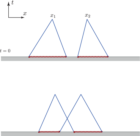
Figure 5: The effect of interaction can be seen in the fermionised representation as dispersion. Large time correlations are determined by the large distance asymptotics of Jordan-Wigner string correlations, which despite their non-local nature, satisfy the clustering property due to the cancellation of overlapping strings.

The non-trivial case is when the set of points is split into subsets of odd number, since then there is one infinitely long string connecting the two subsets (the rightmost operator of the left subset to the leftmost operator of the right subset). While it may be true that clustering of correlations of the local boson field $\hat{\Psi}$ implies also clustering of correlations of the non-local fermion field $\hat{\Phi}$, we will not address this question here. We should mention however that in the only case of initial state for which fermionic correlations have been explicitly calculated, the BEC state, fermionic correlations turn out to satisfy exponential clustering KCC . This is expected to be more generally valid, as we can see by writing the expectation value of the string operator as a cluster expansion

$$\left\langle\exp\left(\mathrm{i}\pi\int_{x}^{y}\mathrm{d}s\,\hat{\rho}(s)\right)\right\rangle =\left\langle:\exp\left(-2\int_{x}^{y}\mathrm{d}s\,\hat{\rho}(s)\right):\right\rangle$$

$$=\exp\left(-2\rho_{0}|x-y|+\sum_{n=2}^{\infty}\frac{(-2)^{n}}{n!}\prod_{i=1}^{n}\int_{x}^{y}ds_{i}\,C_{0}^{\rho}(s_{1},s_{2},...,s_{n})\right)$$ (95)

where

$$C_{0}^{\rho}(x_{1},x_{2},...,x_{n}) =\left\langle:\rho(x_{1})\rho(x_{2})...\rho(x_{n}):\right\rangle$$ (96)

are the normal-ordered connected correlation functions of the density operator. At large distances we find

$$\left\langle\exp\left(\mathrm{i}\pi\int_{x}^{y}\mathrm{d}s\,\hat{\rho}(s)\right)\right\rangle \sim\exp\left[-\left(2\rho_{0}+\sum_{n=2}^{\infty}\frac{(-\text{1})^{n+1}}{n!}\prod_{i=2}^{n}\int_{-\infty}^{+\infty}ds_{i}\,C_{0}^{\rho}(0,s_{2},...,s_{n})\right)|x-y|\right],\quad\text{for }|x-y|\to\infty$$ (97)

The convergence of the integrals in the thermodynamic limit is guaranteed by a sufficiently strong cluster property. Note that this time the required cluster property refers to correlations of the density which is a local field. On ground states of 1D quantum gases the large distance decay of connected density correlations is algebraic. Following a standard result of Luttinger liquid theory Haldane , the decay of the density two-point correlation function is proportional to the inverse square of the distance. Similarly, for higher order correlation functions Luttinger liquid theory gives at most inverse square decay. Therefore each of the above integrals is convergent in ground states of Luttinger liquids. On the other hand, the convergence of the series can be expected to be true at least for sufficiently low densities, since $C_{0}^{\rho}(x_{1},x_{2},...,x_{n})\sim\rho_{0}^{n}$ so the series can be seen as a Taylor expansion in the density.

Appendix C The classical KdV equation and its general solution

In this appendix we give an overview of the general solution of the classical KdV equation and its long time asymptotics. The KdV equation in its standard form is

$$\partial_{t}u(x,t)=6u(x,t)\partial_{x}u(x,t)-\partial_{x}^{3}u(x,t)$$ (98)

As is well-known, this integrable differential equation admits solitary wave solutions. The one-soliton solution is

$$u_{s}(x,t)=-\frac{1}{2}\frac{v_{s}}{\cosh^{2}\left[\tfrac{1}{2}\sqrt{v_{s}}\left(x-v_{s}t-x_{0}\right)\right]}$$ (99)

where $v_{s}>0$ is the soliton velocity and $x_{0}$ is arbitrary. Multi-soliton solutions also exist, as well as dispersive wave solutions.

The general solution to this equation for an arbitrary initial condition is given by the inverse scattering transform, which was actually discovered and first applied to precisely this equation KdV_solution . The inverse scattering approach reduces the above nonlinear equation to two linear problems: finding the spectrum of the Schrödinger equation with an external potential (direct scattering problem) and inversely finding the potential that corresponds to a given spectrum (inverse-scattering problem). In more detail the solution steps are as follows:

1. From the initial condition $u(x,0)$ derive the scattering data of the associated Schrödinger equation

   $$-\frac{d^{2}}{dx^{2}}\psi+u(x,0)\psi=E\psi$$ (100)

   with potential $V(x)=u(x,0)$, i.e. the discrete spectrum $E=-\kappa_{n}^{2}$ corresponding to bound states of the Schrödinger equation, the associated norming (normalisation) constants $c_{n}$ and the reflection coefficient $R(k)$ of the continuous spectrum.

2. Time evolve the scattering data: the discrete spectrum eigenvalues $\kappa_{n}$ remain time invariant, while $c_{n}(t)=c_{n}(0)\mathrm{e}^{A\kappa_{n}^{3}t}$ and $R(k,t)=R(k,0)\mathrm{e}^{\mathrm{i}Bk^{3}t}$.

3. Solve the inverse scattering problem of deriving the time evolved solution $u(x,t)$ as the potential of a Schrödinger equation associated with the time evolved scattering data.

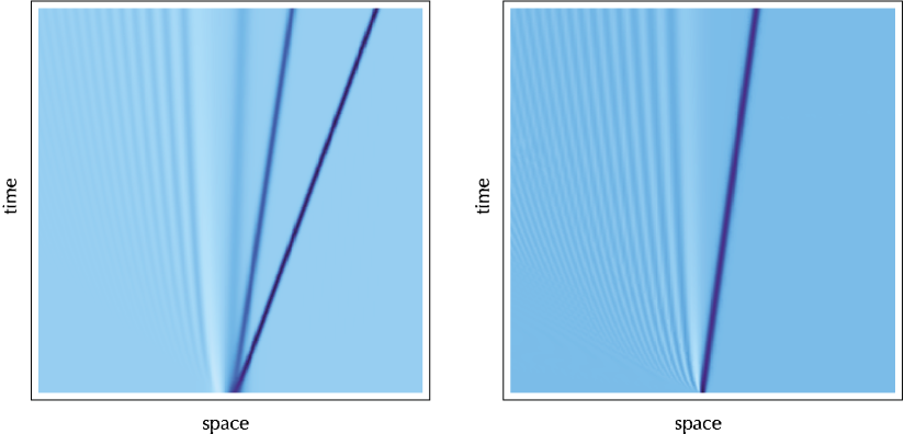
Figure 6: Time evolution of an initial fluctuation following the classical KdV equation. Two different initial conditions are considered: In the general case (left) the evolution leads to decomposition into a number of solitons travelling to one direction and dispersive modes travelling to the opposite. For a single narrowly-localised pulse (right) there is precisely one soliton.

Discrete eigenvalues of the Schrödinger equation correspond to solitary waves, while the continuum part of the spectrum corresponds to dispersive modes. Note that there is at least one discrete eigenvalue for any negative initial condition $u(x,0)$. In the limit of an infinitely narrow localised initial configuration, the Dirac $\delta$-pulse $u(x,0)=-\lambda\delta(x)$, there is precisely one bound state eigenvalue $\kappa=\frac{1}{2}\lambda$.

What we are interested in however is not a formal expression for the general solution, but rather the general form of the long time asymptotics for any initial condition. The power of integrability can be seen in the fact that this partial but most essential information about the solution can be derived without explicitly knowing it. Indeed using the nonlinear steepest descent method, it has be shown that at large times the general solution for any initial condition that is sufficiently fast decaying at spatial infinities, decomposes to a superposition of a finite number of solitons moving at different velocities to the same direction and a decaying in time dispersive part moving to the opposite direction math:KdV_asympt (Fig. 6)

$$u(x,t)\sim\begin{cases}-2\sum_{j=1}^{N}\frac{\kappa_{j}^{2}}{\cosh^{2}(\kappa_{j}x-4\kappa_{j}^{3}t-a_{j})}&,\,x/t>0\\ O\left(t^{-1/2}\right)&,\,x/t<0\end{cases}\quad\text{for }t\to\infty,\,x/t\text{ fixed}$$ (101)

for some suitable phase shifts $a_{j}$.