Optimal discrimination designs for semi-parametric models

Holger Dette
Ruhr-Universität Bochum
Fakultät für Mathematik
44780 Bochum, Germany
e-mail: holger.dette@ruhr-uni-bochum.de
   Roman Guchenko, Viatcheslav Melas
St. Petersburg State University
Faculty of Mathematics and Mechanics
St. Petersburg, Russia
e-mail: romanguchenko@ya.ru, vbmelas@post.ru
   Weng Kee Wong
Department of Biostatistics
UCLA Fielding School of Public Health
Los Angeles, CA 90095-1772
e-mail: wkwong@ucla.edu
Abstract

Much of the work in the literature on optimal discrimination designs assumes that the models of interest are fully specified, apart from unknown parameters in some models. Recent work allows errors in the models to be non-normally distributed but still requires the specification of the mean structures. This research is motivated by the interesting work of Otsu, (2008) to discriminate among semi-parametric models by generalizing the KL-optimality criterion proposed by López-Fidalgo et al., (2007) and Tommasi and López-Fidalgo, (2010). In our work we provide further important insights in this interesting optimality criterion. In particular, we propose a practical strategy for finding optimal discrimination designs among semi-parametric models that can also be verified using an equivalence theorem. In addition, we study properties of such optimal designs and identify important cases where the proposed semi-parametric optimal discrimination designs coincide with the celebrated T𝑇T-optimal designs.

Keywords and Phrases: continuous design, discrimination design, equivalence theorem, semi-parametric model, T𝑇T-optimality, variational calculus.

1 Introduction

Finding optimal discrimination designs dates back to 1970’s and probably earlier. Early references are Stigler, (1971) who considered nested models and Atkinson and Fedorov, 1975a ; Atkinson and Fedorov, 1975b , where they proposed T𝑇T-optimal designs to discriminate among models when errors are normally distributed. The first of the two last named papers concerns discrimination between two models and the second paper generalized the problem to multiple models. T𝑇T-optimality for discriminating between parametric models assumes that we have a known null model and we wish to test whether a rival model with unknown parameter holds. A likelihood ratio test is then used to discriminate between the two rival models and under local alternatives, the non-centrality parameter of the chi-square distribution of the test statistic, which contains the unknown parameters from the alternative model, is proportional to the T𝑇T-optimality criterion (Wiens, , 2009). Since a larger non-centrality parameter provides a more powerful test, the T𝑇T-optimal design strategy is to find a design that maximizes the minimum value of the non-centrality parameter, where the minimum is taken over all possible values of the parameters in the model under the alternative hypothesis. Consequently, T𝑇T-optimality criterion is a type of maximin optimality criterion and designs that maximize the minimum of the non-centrality parameter are called T𝑇T-optimal designs.

The two seminal papers of Atkinson and Fedorov, 1975a ; Atkinson and Fedorov, 1975b contain illustrative examples. Because the T𝑇T-optimality criterion is not differentiable, calculations to determine the optimal design can be involved even for relatively simple models; see for example, Dette et al., (2012) and Dette et al., 2016b for some explicit non-trivial results. For the same reason, the construction of efficient algorithms for finding T𝑇T-optimal designs is a challenging problem. Some recent progress in this direction includes Braess and Dette, (2013); Dette et al., (2015); Dette et al., 2016a and Tommasi et al., (2016). An interactive software tool for finding optimal discrimination designs is available in Stegmaier et al., (2013).

There is notable progress in tackling optimal discrimination design problems on various fronts; the progress appeared periodic a few decades ago and seems to have picked up in recent years. Advances include alternative problem formulations and broader applications of such designs in cognitive science (Covagnaro et al., , 2010), psychology (Myung and Pitt, , 2009) and chemical engineering (Alberton et al., , 2011), to name a few. Different and more flexible optimality criteria have also been proposed. In particular, advances in the construction of optimal discrimination designs include the following: (i) the frequently criticized unrealistic assumption in the T𝑇T-optimality criterion that requires a known model in the null hypothesis is now removed (Jamsen et al., , 2013); (ii) the class of models of interest now includes generalized linear models, where outcomes can be discrete (Waterhouse et al., , 2008), (iii) optimal designs for discriminating multivariate models (Yanagisawa, , 1990; Ucinski and Bogacka, , 2005); (iv) Bayesian optimal designs for model discrimination (Felsenstein, , 1992; Tommasi and López-Fidalgo, , 2010; Dette et al., , 2015) , (v) dual-objective optimal designs for model discrimination (Atkinson et al., , 1998; Ng and Chick, , 2004; Atkinson, , 2008; Alberton et al., , 2011; Abd El-Monsef and Seyam, , 2011), (vi) discriminating models with correlated errors (Campos-Barreiro and Lopez-Fidalgo, , 2016), (vii) adaptive designs for model discrimination (Myung and Pitt, , 2009; Donckels et al., , 2009) and (viii) optimal discrimination designs for dynamic models (Ucinski and Bogacka, , 2005). Other important references that describe alternative approaches and properties of optimal discrimination designs are López-Fidalgo et al., (2007); Dette and Titoff, (2009); Dette et al., (2015), among others.

All references cited so far require a parametric specification of the conditional distribution of the response, which raises some robustness issues in the application of the T𝑇T-optimality criterion for constructing optimal discrimination designs. Robustness properties of optimal discrimination designs with respect to various model assumptions have been considered by Wiens, (2009); Ghosh and Dutta, (2013) and Dette et al., (2013). Otsu, (2008) proposed a new optimality criterion for discriminating between models, which is similar in spirit to the classical T𝑇T-optimality criterion and its extensions except that it does not require an exact specification of the conditional distribution. Optimal discrimination designs were found using the duality relationships in entropy-like minimization problems (Borwein and Lewis, , 1991) and the resulting optimal designs are called semi-parametric optimal discrimination designs.

The present paper provides a more careful analysis of the novel approach proposed by Otsu, (2008). We propose a more practical strategy for finding semi-parametric optimal discrimination designs and derive several important properties of such optimal designs. In Section 2, we define semi-parametric optimal discrimination designs and derive several auxiliary results that substantially simplify the calculation of optimal designs. In Section 3, we provide equivalence theorems to characterize semi-parametric optimal discrimination designs and demonstrate that all designs derived by Otsu, (2008) are in fact not optimal. Section 4 describes the relation between semi-parametric optimal discrimination designs and optimal discrimination designs under some criteria discussed in the literature. In particular, we identify cases, where the semi-parametric optimal discrimination designs proposed by Otsu, (2008) coincide with the T𝑇T-optimal discrimination designs and KL-optimal designs introduced by Atkinson and Fedorov, 1975a ; Atkinson and Fedorov, 1975b and López-Fidalgo et al., (2007), respectively. Section 5 presents numerical results and all technical details are deferred to the appendix in Section 6.

2 Semi-parametric discrimination designs

We model the response variable Y𝑌Y as a function of a vector of explanatory variables x𝑥x defined on a given compact design space 𝒳𝒳\mathcal{X}. Suppose the density of Y𝑌Y with respect to the Lebesgue measure is f(y,x)𝑓𝑦𝑥f(y,x), and we have resources to take a fixed number of observations, say n𝑛n, for the study. Following Kiefer, (1974), we focus on approximate designs which are essentially probability measures defined on 𝒳𝒳\mathcal{X}. If an approximate design has k𝑘k support points, say x1,,xksubscript𝑥1subscript𝑥𝑘x_{1},\ldots,x_{k}, and the corresponding weights are ω1,,ωksubscript𝜔1subscript𝜔𝑘\omega_{1},\ldots,\omega_{k}, then approximately nωi𝑛subscript𝜔𝑖n\omega_{i} observations are taken at xi,i=1,,kformulae-sequencesubscript𝑥𝑖𝑖1𝑘x_{i},i=1,\ldots,k. In practice, a rounding procedure is applied to every nωi𝑛subscript𝜔𝑖n\omega_{i} so that they are positive integers nisubscript𝑛𝑖n_{i} (i=1,,k)i=1,\ldots,k) and i=1kni=nsuperscriptsubscript𝑖1𝑘subscript𝑛𝑖𝑛\sum_{i=1}^{k}n_{i}=n. The experimenter then takes nisubscript𝑛𝑖n_{i} independent observations with Yi,1,,Yi,nisubscript𝑌𝑖1subscript𝑌𝑖subscript𝑛𝑖Y_{i,1},\ldots,Y_{i,n_{i}} at xisubscript𝑥𝑖x_{i} which are assumed to have a density f(y,xi)𝑓𝑦subscript𝑥𝑖f(y,x_{i}) with respect to the Lebesgue measure, i=1,,k𝑖1𝑘i=1,\ldots,k.

To construct efficient designs for discriminating between two competing models for f(y,x)𝑓𝑦𝑥f(y,x), López-Fidalgo et al., (2007) assumed parametric densities, say fj(y,x,θj)subscript𝑓𝑗𝑦𝑥subscript𝜃𝑗f_{j}(y,x,\theta_{j}), where the parameter θjsubscript𝜃𝑗\theta_{j} varies in a compact parameter space, say Θj,subscriptΘ𝑗\Theta_{j}, j=1,2𝑗12j=1,2. To fix ideas, we ignore nuisance parameters which may be present in the models. The Kullback-Leibler distance between two densities f1subscript𝑓1f_{1} and f2subscript𝑓2f_{2} is

I1,2(x,f1,f2,θ1,θ2)=f1(y,x,θ1)logf1(y,x,θ1)f2(y,x,θ2)dysubscript𝐼12𝑥subscript𝑓1subscript𝑓2subscript𝜃1subscript𝜃2subscript𝑓1𝑦𝑥subscript𝜃1subscript𝑓1𝑦𝑥subscript𝜃1subscript𝑓2𝑦𝑥subscript𝜃2𝑑𝑦I_{1,2}(x,f_{1},f_{2},\theta_{1},\theta_{2})=\int f_{1}(y,x,\theta_{1})\log\frac{f_{1}(y,x,\theta_{1})}{f_{2}(y,x,\theta_{2})}dy (2.1)

and it measures the discrepancy between the densities. López-Fidalgo et al., (2007) assumed that the model f1subscript𝑓1f_{1} is the “true” model with a fixed parameter vector θ¯1subscript¯𝜃1\overline{\theta}_{1} and call a design local KL-optimal discriminating design for the models f1subscript𝑓1f_{1} and f2subscript𝑓2f_{2} if it maximizes the criterion

KL1,2(ξ,θ¯1)=infθ2Θ2𝒳I1,2(x,f1,f2,θ¯1,θ2)ξ(dx).subscriptKL12𝜉subscript¯𝜃1subscriptinfimumsubscript𝜃2subscriptΘ2subscript𝒳subscript𝐼12𝑥subscript𝑓1subscript𝑓2subscript¯𝜃1subscript𝜃2𝜉𝑑𝑥\mathrm{KL}_{1,2}(\xi,\overline{\theta}_{1})=\inf_{\theta_{2}\in\Theta_{2}}\int_{\mathcal{X}}I_{1,2}(x,f_{1},f_{2},{\overline{\theta}_{1}},\theta_{2})\xi(dx). (2.2)

Otsu, (2008) considered a novel setup and proposed a design criterion for discriminating a parametric model defined by its density and another nonparametric model. More precisely, this author considered the design problem for testing the hypothesis

H0:η(x)=η1(x,θ1)versusH1:η(x)=η2(x,θ2):subscript𝐻0𝜂𝑥subscript𝜂1𝑥subscript𝜃1versussubscript𝐻1:𝜂𝑥subscript𝜂2𝑥subscript𝜃2H_{0}:\eta(x)=\eta_{1}(x,\theta_{1})\leavevmode\nobreak\ \leavevmode\nobreak\ \mbox{versus}\leavevmode\nobreak\ \leavevmode\nobreak\ H_{1}:\eta(x)=\eta_{2}(x,\theta_{2}) (2.3)

where

ηj(x,θj)=yfj(y,x,θj)𝑑y,j=1,2,formulae-sequencesubscript𝜂𝑗𝑥subscript𝜃𝑗𝑦subscript𝑓𝑗𝑦𝑥subscript𝜃𝑗differential-d𝑦𝑗12\eta_{j}(x,\theta_{j})=\int yf_{j}(y,x,\theta_{j})dy,\;j=1,2,

is the conditional mean of the density fj(y,x,θj)subscript𝑓𝑗𝑦𝑥subscript𝜃𝑗f_{j}(y,x,\theta_{j}) with support set

𝒮fj,θj,x={y|fj(y,x,θj)>0},j=1,2.formulae-sequencesubscript𝒮subscript𝑓𝑗subscript𝜃𝑗𝑥conditional-set𝑦subscript𝑓𝑗𝑦𝑥subscript𝜃𝑗0𝑗12{\cal S}_{f_{j},\theta_{j},x}=\big{\{}y\leavevmode\nobreak\ |\leavevmode\nobreak\ f_{j}(y,x,\theta_{j})>0\big{\}}\leavevmode\nobreak\ ,\leavevmode\nobreak\ \leavevmode\nobreak\ j=1,2. (2.4)

The setup is therefore more general than that in López-Fidalgo et al., (2007), who assumed that f1subscript𝑓1f_{1} and f2subscript𝑓2f_{2} are known and one of the parametric models is fully specified. To be more specific, let f1(y,x,θ¯1)subscript𝑓1𝑦𝑥subscript¯𝜃1f_{1}(y,x,\overline{\theta}_{1}) be a parametric density with a fixed parameter θ¯1subscript¯𝜃1\overline{\theta}_{1} and define

2,x,θ2={f2:f2(y,x,θ2)𝑑y=1,yf2(y,x,θ2)𝑑y=η2(x,θ2),𝒮f2,θ2,x=𝒮f1,θ¯1,x},subscript2𝑥subscript𝜃2conditional-setsubscript𝑓2formulae-sequencesubscript𝑓2𝑦𝑥subscript𝜃2differential-d𝑦1formulae-sequence𝑦subscript𝑓2𝑦𝑥subscript𝜃2differential-d𝑦subscript𝜂2𝑥subscript𝜃2subscript𝒮subscript𝑓2subscript𝜃2𝑥subscript𝒮subscript𝑓1subscript¯𝜃1𝑥\displaystyle\mathcal{F}_{2,x,\theta_{2}}=\Big{\{}f_{2}:\int f_{2}(y,x,\theta_{2})\,dy=1,\;\int yf_{2}(y,x,\theta_{2})dy=\eta_{2}(x,\theta_{2}),\leavevmode\nobreak\ \mathcal{S}_{f_{2},\theta_{2},x}=\mathcal{S}_{f_{1},\overline{\theta}_{1},x}\Big{\}}, (2.5)

which is the class of all conditional densities (at the point x𝑥x) with parameter θ2subscript𝜃2\theta_{2} and conditional mean η2(x,θ2)subscript𝜂2𝑥subscript𝜃2\eta_{2}(x,\theta_{2}). Consider the set obtained from 2,x,θ2subscript2𝑥subscript𝜃2\mathcal{F}_{2,x,\theta_{2}} by letting the ranges of x𝑥x and θ2subscript𝜃2\theta_{2} vary over all their possible values:

2={2,x,θ2|x𝒳;θ2Θ2}subscript2conditional-setsubscript2𝑥subscript𝜃2formulae-sequence𝑥𝒳subscript𝜃2subscriptΘ2\displaystyle\mathcal{F}_{2}=\big{\{}\mathcal{F}_{2,x,\theta_{2}}\leavevmode\nobreak\ |\leavevmode\nobreak\ x\in{\cal X};\leavevmode\nobreak\ \theta_{2}\in\Theta_{2}\big{\}}

and call a design ξsuperscript𝜉\xi^{*} semi-parametric optimal design for discriminating between the model f1(y,x,θ¯1)subscript𝑓1𝑦𝑥subscript¯𝜃1f_{1}(y,x,\overline{\theta}_{1}) and models in the class 2subscript2\mathcal{F}_{2} if it maximizes the optimality criterion

K(a)(ξ,θ¯1)=infθ2Θ2Xinff22,x,θ2I1,2(x,f1,f2,θ¯1,θ2)ξ(dx)subscript𝐾𝑎𝜉subscript¯𝜃1subscriptinfimumsubscript𝜃2subscriptΘ2subscript𝑋subscriptinfimumsubscript𝑓2subscript2𝑥subscript𝜃2subscript𝐼12𝑥subscript𝑓1subscript𝑓2subscript¯𝜃1subscript𝜃2𝜉𝑑𝑥\displaystyle K_{(a)}(\xi,{\overline{\theta}_{1}})=\inf_{\theta_{2}\in\Theta_{2}}\int_{X}\inf_{f_{2}\in\mathcal{F}_{2,x,\theta_{2}}}I_{1,2}(x,f_{1},f_{2},{\overline{\theta}_{1}},\theta_{2})\,\xi(dx) (2.6)

among all approximate designs defined on the design space 𝒳𝒳{\cal X}. Note that this criterion is a local optimality criterion in the sense of Chernoff, (1953) as it depends on the parameter θ¯1subscript¯𝜃1\overline{\theta}_{1}. The subscript (a)𝑎(a) denotes the first design criterion with the subscript (b)𝑏(b) for the second design criterion below.
Similarly, we may fix the conditional density f2(y,x,θ2)subscript𝑓2𝑦𝑥subscript𝜃2f_{2}(y,x,\theta_{2}) and define

1,x,θ¯1subscript1𝑥subscript¯𝜃1\displaystyle\mathcal{F}_{1,x,\overline{\theta}_{1}} ={f1:f1(y,x,θ¯1)𝑑y=1,yf1(y,x,θ¯1)𝑑y=η1(x,θ¯1),𝒮f1,θ¯1,x=𝒮f2,θ2,x},absentconditional-setsubscript𝑓1formulae-sequencesubscript𝑓1𝑦𝑥subscript¯𝜃1differential-d𝑦1formulae-sequence𝑦subscript𝑓1𝑦𝑥subscript¯𝜃1differential-d𝑦subscript𝜂1𝑥subscript¯𝜃1subscript𝒮subscript𝑓1subscript¯𝜃1𝑥subscript𝒮subscript𝑓2subscript𝜃2𝑥\displaystyle=\Big{\{}f_{1}:\int f_{1}(y,x,{\overline{\theta}_{1}})\,dy=1,\int yf_{1}(y,x,{\overline{\theta}_{1}}){dy}=\eta_{1}(x,{\overline{\theta}_{1}}),\leavevmode\nobreak\ \mathcal{S}_{f_{1},\overline{\theta}_{1},x}=\mathcal{S}_{f_{2},\theta_{2},x}\Big{\}}, (2.7)

which is the class of all conditional densities with parameter θ¯1subscript¯𝜃1\overline{\theta}_{1} and conditional mean η1(x,θ¯1)subscript𝜂1𝑥subscript¯𝜃1\eta_{1}(x,\overline{\theta}_{1}). For fixed θ¯1subscript¯𝜃1\overline{\theta}_{1}, let

1subscript1\displaystyle\mathcal{F}_{1} ={1,x,θ¯1|x𝒳}absentconditional-setsubscript1𝑥subscript¯𝜃1𝑥𝒳\displaystyle=\big{\{}\mathcal{F}_{1,x,\overline{\theta}_{1}}\leavevmode\nobreak\ |\leavevmode\nobreak\ x\in{\cal X}\big{\}}

and we call a design ξ𝜉\xi locally semi-parametric optimal design for discriminating between the model f2(y,x,θ2)subscript𝑓2𝑦𝑥subscript𝜃2f_{2}(y,x,\theta_{2}) and the class 1subscript1\mathcal{F}_{1} if it maximizes the optimality criterion

K(b)(ξ,θ¯1)=infθ2Θ2Xinff11,x,θ¯1I1,2(x,f1,f2,θ¯1,θ2)ξ(dx),subscript𝐾𝑏𝜉subscript¯𝜃1subscriptinfimumsubscript𝜃2subscriptΘ2subscript𝑋subscriptinfimumsubscript𝑓1subscript1𝑥subscript¯𝜃1subscript𝐼12𝑥subscript𝑓1subscript𝑓2subscript¯𝜃1subscript𝜃2𝜉𝑑𝑥\displaystyle K_{(b)}(\xi,{\overline{\theta}_{1}})=\inf_{\theta_{2}\in\Theta_{2}}\int_{X}\inf_{f_{1}\in\mathcal{F}_{1,x,\overline{\theta}_{1}}}I_{1,2}(x,f_{1},f_{2},{\overline{\theta}_{1}},\theta_{2})\,\xi(dx), (2.8)

among all approximate designs defined on the design space 𝒳𝒳{\cal X}.

Remark 2.1

We note that the above approach can be similarly applied when the response variable Y𝑌Y is discrete and it has one of two possible discrete probability measures that depends on x𝑥x and θ¯1subscript¯𝜃1\overline{\theta}_{1}. Let these two competing measures with the same support be

P(x,θ¯1)=[y1(x,θ¯1)ys(x,θ¯1)p1(x,θ¯1)ps(x,θ¯1)]andQ(x,θ2)=[y1(x,θ¯1)ys(x,θ¯1)q1(x,θ2)qs(x,θ2)].𝑃𝑥subscript¯𝜃1matrixsubscript𝑦1𝑥subscript¯𝜃1subscript𝑦𝑠𝑥subscript¯𝜃1subscript𝑝1𝑥subscript¯𝜃1subscript𝑝𝑠𝑥subscript¯𝜃1and𝑄𝑥subscript𝜃2matrixsubscript𝑦1𝑥subscript¯𝜃1subscript𝑦𝑠𝑥subscript¯𝜃1subscript𝑞1𝑥subscript𝜃2subscript𝑞𝑠𝑥subscript𝜃2\displaystyle P(x,\overline{\theta}_{1})=\begin{bmatrix}y_{1}(x,\overline{\theta}_{1})&\dots&y_{s}(x,\overline{\theta}_{1})\\ p_{1}(x,\overline{\theta}_{1})&\dots&p_{s}(x,\overline{\theta}_{1})\end{bmatrix}\;\leavevmode\nobreak\ \text{and}\leavevmode\nobreak\ Q(x,\theta_{2})=\begin{bmatrix}y_{1}(x,\overline{\theta}_{1})&\dots&y_{s}(x,\overline{\theta}_{1})\\ q_{1}(x,\theta_{2})&\dots&q_{s}(x,\theta_{2})\end{bmatrix}.

If we let yi=yi(x,θ¯1)subscript𝑦𝑖subscript𝑦𝑖𝑥subscript¯𝜃1y_{i}=y_{i}(x,\overline{\theta}_{1}), let pi=pi(x,θ¯1)subscript𝑝𝑖subscript𝑝𝑖𝑥subscript¯𝜃1p_{i}=p_{i}(x,\overline{\theta}_{1}) and let qi=qi(x,θ2)subscript𝑞𝑖subscript𝑞𝑖𝑥subscript𝜃2q_{i}=q_{i}(x,\theta_{2}) for simplicity, we have i=1spi=1=i=1sqisuperscriptsubscript𝑖1𝑠subscript𝑝𝑖1superscriptsubscript𝑖1𝑠subscript𝑞𝑖\sum_{i=1}^{s}p_{i}=1=\sum_{i=1}^{s}q_{i} and i=1syipi=η1(x,θ¯1)superscriptsubscript𝑖1𝑠subscript𝑦𝑖subscript𝑝𝑖subscript𝜂1𝑥subscript¯𝜃1\sum_{i=1}^{s}y_{i}p_{i}=\eta_{1}(x,\overline{\theta}_{1}). Define two sets

Qx,θ2={q:i=1sqi=1,i=1syiqi=η2, 0<qi1}andQ={Qx,θ2|x𝒳;θ2Θ2}.subscript𝑄𝑥subscript𝜃2conditional-set𝑞formulae-sequencesuperscriptsubscript𝑖1𝑠subscript𝑞𝑖1formulae-sequencesuperscriptsubscript𝑖1𝑠subscript𝑦𝑖subscript𝑞𝑖subscript𝜂2 0subscript𝑞𝑖1and𝑄conditional-setsubscript𝑄𝑥subscript𝜃2formulae-sequence𝑥𝒳subscript𝜃2subscriptΘ2\displaystyle Q_{x,\theta_{2}}=\Big{\{}q:\sum_{i=1}^{s}q_{i}=1,\;\sum_{i=1}^{s}y_{i}q_{i}=\eta_{2},\;0<q_{i}\leq 1\Big{\}}\ \text{and}\leavevmode\nobreak\ Q=\Big{\{}Q_{x,\theta_{2}}\leavevmode\nobreak\ |\leavevmode\nobreak\ x\in{\cal X};\leavevmode\nobreak\ \theta_{2}\in\Theta_{2}\Big{\}}.

To find a semi-parametric optimal design ξsuperscript𝜉\xi^{*} for discriminating between the model P(x,θ¯1)𝑃𝑥subscript¯𝜃1P(x,\overline{\theta}_{1}) and the class Q𝑄Q we may use the discrete version of the criterion (2.6), which is

K~(a)(ξ,θ¯1)=infθ2Θ2XinfqQx,θ2i=1spi(x,θ¯1)logpi(x,θ¯1)qi(x,θ2)ξ(dx).subscript~𝐾𝑎𝜉subscript¯𝜃1subscriptinfimumsubscript𝜃2subscriptΘ2subscript𝑋subscriptinfimum𝑞subscript𝑄𝑥subscript𝜃2superscriptsubscript𝑖1𝑠subscript𝑝𝑖𝑥subscript¯𝜃1subscript𝑝𝑖𝑥subscript¯𝜃1subscript𝑞𝑖𝑥subscript𝜃2𝜉𝑑𝑥\displaystyle\tilde{K}_{(a)}(\xi,{\overline{\theta}_{1}})=\inf_{\theta_{2}\in\Theta_{2}}\int_{X}\inf_{q\in Q_{x,\theta_{2}}}\sum_{i=1}^{s}p_{i}(x,\overline{\theta}_{1})\log{\frac{p_{i}(x,\overline{\theta}_{1})}{q_{i}(x,\theta_{2})}}\,\xi(dx).

We then write down the discrete version of (2.8) in a similar manner and proceed, omitting details for space consideration.

In what is to follow, we assume for simplicity that f1(y,x,θ1)subscript𝑓1𝑦𝑥subscript𝜃1f_{1}(y,x,\theta_{1}), f2(y,x,θ2)subscript𝑓2𝑦𝑥subscript𝜃2f_{2}(y,x,\theta_{2}), η1(x,θ1)subscript𝜂1𝑥subscript𝜃1\eta_{1}(x,\theta_{1}), η2(x,θ2)subscript𝜂2𝑥subscript𝜃2\eta_{2}(x,\theta_{2}) are differentiable with respect to y𝑦y, x𝑥x, θ1subscript𝜃1\theta_{1} and θ2subscript𝜃2\theta_{2}, even though these assumptions can be weakened a bit for what we plan to do here. Otsu, (2008) derived an explicit form for the two criteria. For the criterion (2.6), he obtained

K(a)(ξ,θ¯1)=infθ2Θ2X{μ+1+log{μλ(yη2(x,θ2))}f1(y,x,θ¯1)𝑑y}ξ(dx),subscript𝐾𝑎𝜉subscript¯𝜃1subscriptinfimumsubscript𝜃2subscriptΘ2subscript𝑋𝜇1𝜇𝜆𝑦subscript𝜂2𝑥subscript𝜃2subscript𝑓1𝑦𝑥subscript¯𝜃1differential-d𝑦𝜉𝑑𝑥\displaystyle K_{(a)}(\xi,{\overline{\theta}_{1}})=\inf_{\theta_{2}\in\Theta_{2}}\int_{X}\left\{\mu+1+\int\log\left\{-\mu-\lambda(y-\eta_{2}(x,\theta_{2}))\right\}f_{1}(y,x,{\overline{\theta}_{1}})dy\right\}\xi(dx),

where the constants λ𝜆\lambda and μ𝜇\mu depend on x𝑥x , θ¯1subscript¯𝜃1\overline{\theta}_{1} and θ2subscript𝜃2\theta_{2} and are roots of the system of equations

f1(y,x,θ¯1)μ+λ(yη2(x,θ2))𝑑y=1,(yη2(x,θ2))f1(y,x,θ¯1)μ+λ(yη2(x,θ2))𝑑y=0formulae-sequencesubscript𝑓1𝑦𝑥subscript¯𝜃1𝜇𝜆𝑦subscript𝜂2𝑥subscript𝜃2differential-d𝑦1𝑦subscript𝜂2𝑥subscript𝜃2subscript𝑓1𝑦𝑥subscript¯𝜃1𝜇𝜆𝑦subscript𝜂2𝑥subscript𝜃2differential-d𝑦0\displaystyle-\int\frac{f_{1}(y,x,{\overline{\theta}_{1}})}{\mu+\lambda(y-\eta_{2}(x,\theta_{2}))}dy=1,\;\int\frac{(y-\eta_{2}(x,\theta_{2}))f_{1}(y,x,{\overline{\theta}_{1}})}{\mu+\lambda(y-\eta_{2}(x,\theta_{2}))}dy=0

that satisfy the constraint

μ+λ(yη2(x,θ2))<0, for all y𝒮f1,θ¯1,x.formulae-sequence𝜇𝜆𝑦subscript𝜂2𝑥subscript𝜃20 for all 𝑦subscript𝒮subscript𝑓1subscript¯𝜃1𝑥\displaystyle\mu+\lambda(y-\eta_{2}(x,\theta_{2}))<0,\;\mbox{\leavevmode\nobreak\ for all \leavevmode\nobreak\ }y\in{\cal S}_{f_{1},\overline{\theta}_{1},x}.

A similar result can be obtained for the criterion (2.8) using somewhat similar arguments and they are omitted for space consideration. In either case, the desired values for μ𝜇\mu and λ𝜆\lambda have to be found numerically. Otsu, (2008) did not provide an effective numerical procedure for finding solutions in the two dimensional space that solve the system of equations and satisfy the constraint. In what is to follow, we show that the inner optimization problems in (2.6) and (2.8) can be reduced to solving a single equation, which is much faster and more reliable. For this purpose we derive simpler expressions for the criteria (2.6) and (2.8) that facilitate the computation of the semi-parametric optimal discriminating designs. One of our key results is the following.

Theorem 2.1

(a) Assume that for each x𝒳𝑥𝒳x\in\mathcal{X} the support of the conditional density f1(y,x,θ¯1)subscript𝑓1𝑦𝑥subscript¯𝜃1f_{1}(y,x,\overline{\theta}_{1}) is an interval, i.e. 𝒮f1,θ¯1,x=[yx,min,yx,max]subscript𝒮subscript𝑓1subscript¯𝜃1𝑥subscript𝑦𝑥subscript𝑦𝑥{\cal S}_{f_{1},\overline{\theta}_{1},x}=[y_{x,\min},y_{x,\max}], such that yx,min<η2(x,θ2)<yx,maxsubscript𝑦𝑥subscript𝜂2𝑥subscript𝜃2subscript𝑦𝑥y_{x,\min}<\eta_{2}(x,\theta_{2})<y_{x,\max} for all θ2Θ2subscript𝜃2subscriptΘ2\theta_{2}\in\Theta_{2}. Assume further that for all x𝒳𝑥𝒳x\in\mathcal{X} and for all θ2Θ2subscript𝜃2subscriptΘ2\theta_{2}\in\Theta_{2} there exists a unique non-zero solution λ¯(x,θ¯1,θ2)¯𝜆𝑥subscript¯𝜃1subscript𝜃2\overline{\lambda}(x,\overline{\theta}_{1},\theta_{2}) of the equation

f1(y,x,θ¯1)1+λ(yη2(x,θ2))𝑑y=1,subscript𝑓1𝑦𝑥subscript¯𝜃11𝜆𝑦subscript𝜂2𝑥subscript𝜃2differential-d𝑦1\displaystyle\int\frac{f_{1}(y,x,\overline{\theta}_{1})}{1+\lambda(y-\eta_{2}(x,\theta_{2}))}dy=1, (2.9)

that satisfies

1yx,maxη2(x,θ2)<λ¯(x,θ¯1,θ2)<1yx,minη2(x,θ2).1subscript𝑦𝑥subscript𝜂2𝑥subscript𝜃2¯𝜆𝑥subscript¯𝜃1subscript𝜃21subscript𝑦𝑥subscript𝜂2𝑥subscript𝜃2\displaystyle-\frac{1}{y_{x,\max}-\eta_{2}{(x,\theta_{2})}}<\overline{\lambda}(x,\overline{\theta}_{1},\theta_{2})<-\frac{1}{y_{x,\min}-\eta_{2}(x,\theta_{2})}. (2.10)

The criterion (2.6) then takes the form

K(a)(ξ,θ¯1)subscript𝐾𝑎𝜉subscript¯𝜃1\displaystyle K_{(a)}(\xi,\overline{\theta}_{1}) =infθ2Θ2𝒳log{1+λ¯(x,θ¯1,θ2)(yη2(x,θ2))}f1(y,x,θ¯1)𝑑yξ(dx)absentsubscriptinfimumsubscript𝜃2subscriptΘ2subscript𝒳1¯𝜆𝑥subscript¯𝜃1subscript𝜃2𝑦subscript𝜂2𝑥subscript𝜃2subscript𝑓1𝑦𝑥subscript¯𝜃1differential-d𝑦𝜉𝑑𝑥\displaystyle=\inf_{\theta_{2}\in\Theta_{2}}\int_{\mathcal{X}}\int\log\left\{1+\overline{\lambda}(x,\overline{\theta}_{1},\theta_{2})(y-\eta_{2}(x,\theta_{2}))\right\}f_{1}(y,x,\overline{\theta}_{1})dy\xi(dx) (2.11)

and the “optimal” density f2superscriptsubscript𝑓2f_{2}^{*} in (2.6) is given by

f2(y,x,θ2)=f1(y,x,θ¯1)1+λ¯(x,θ¯1,θ2)(yη2(x,θ2)).superscriptsubscript𝑓2𝑦𝑥subscript𝜃2subscript𝑓1𝑦𝑥subscript¯𝜃11¯𝜆𝑥subscript¯𝜃1subscript𝜃2𝑦subscript𝜂2𝑥subscript𝜃2\displaystyle f_{2}^{*}(y,x,\theta_{2})=\frac{f_{1}(y,x,\overline{\theta}_{1})}{1+\overline{\lambda}(x,\overline{\theta}_{1},\theta_{2})(y-\eta_{2}(x,\theta_{2}))}. (2.12)

(b) Assume that the integrals

f2(y,x,θ2)exp(λy)𝑑y and yf2(y,x,θ2)exp(λy)𝑑ysubscript𝑓2𝑦𝑥subscript𝜃2𝜆𝑦differential-d𝑦 and 𝑦subscript𝑓2𝑦𝑥subscript𝜃2𝜆𝑦differential-d𝑦\displaystyle\int f_{2}(y,x,\theta_{2})\exp(-\lambda y)dy\leavevmode\nobreak\ \mbox{ and }\leavevmode\nobreak\ \int yf_{2}(y,x,\theta_{2})\exp(-\lambda y)dy

exist for all x𝒳𝑥𝒳x\in\mathcal{X} and for all λ𝜆\lambda. The criterion (2.8) takes the form

K(b)(ξ)=infθ2Θ2𝒳[log{μ(λ¯x)}λ¯xy]f2(y,x,θ2)exp(λ¯xy)μ(λ¯x)𝑑yξ(dx)subscript𝐾𝑏𝜉subscriptinfimumsubscript𝜃2subscriptΘ2subscript𝒳delimited-[]superscript𝜇subscript¯𝜆𝑥subscript¯𝜆𝑥𝑦subscript𝑓2𝑦𝑥subscript𝜃2subscript¯𝜆𝑥𝑦superscript𝜇subscript¯𝜆𝑥differential-d𝑦𝜉𝑑𝑥\displaystyle K_{(b)}(\xi)=\inf_{\theta_{2}\in\Theta_{2}}\int_{\mathcal{X}}\int\left[\log\left\{\mu^{\prime}(\overline{\lambda}_{x})\right\}-\overline{\lambda}_{x}y\right]f_{2}(y,x,\theta_{2})\exp(-\overline{\lambda}_{x}y)\mu^{\prime}(\overline{\lambda}_{x})dy\xi(dx) (2.13)

where

μ(λ)=μ(λ,x,θ2)=1f2(y,x,θ2)exp(λy)𝑑ysuperscript𝜇𝜆superscript𝜇𝜆𝑥subscript𝜃21subscript𝑓2𝑦𝑥subscript𝜃2𝜆𝑦differential-d𝑦\displaystyle\mu^{\prime}(\lambda)=\mu^{\prime}(\lambda,x,\theta_{2})=\frac{1}{\int f_{2}(y,x,\theta_{2})\exp(-\lambda y)dy} (2.14)

and λ¯x=λ¯(x,θ¯1,θ2)subscript¯𝜆𝑥¯𝜆𝑥subscript¯𝜃1subscript𝜃2\overline{\lambda}_{x}=\overline{\lambda}(x,\overline{\theta}_{1},\theta_{2}) is the nonzero root of the equation

yf2(y,x,θ2)exp(λy)𝑑yf2(y,x,θ2)exp(λy)𝑑y=η1(x,θ¯1).𝑦subscript𝑓2𝑦𝑥subscript𝜃2𝜆𝑦differential-d𝑦subscript𝑓2𝑦𝑥subscript𝜃2𝜆𝑦differential-d𝑦subscript𝜂1𝑥subscript¯𝜃1\displaystyle\frac{\int yf_{2}(y,x,\theta_{2})\exp(-\lambda y)dy}{\int f_{2}(y,x,\theta_{2})\exp(-\lambda y)dy}=\eta_{1}(x,\overline{\theta}_{1}). (2.15)

Moreover, the “optimal” density f1superscriptsubscript𝑓1f_{1}^{*} in (2.8) is given by

f1(y,x,θ¯1)=f2(y,x,θ2)exp(λ¯(x,θ¯1,θ2)y)f2(y,x,θ2)exp(λ¯(x,θ¯1,θ2)y)𝑑y.superscriptsubscript𝑓1𝑦𝑥subscript¯𝜃1subscript𝑓2𝑦𝑥subscript𝜃2¯𝜆𝑥subscript¯𝜃1subscript𝜃2𝑦subscript𝑓2𝑦𝑥subscript𝜃2¯𝜆𝑥subscript¯𝜃1subscript𝜃2𝑦differential-d𝑦\displaystyle f_{1}^{*}(y,x,\overline{\theta}_{1})=\frac{f_{2}(y,x,\theta_{2})\exp(-\overline{\lambda}(x,{\overline{\theta}_{1}},\theta_{2})y)}{\int f_{2}(y,x,\theta_{2})\exp(-\overline{\lambda}(x,\overline{\theta}_{1},\theta_{2})y)dy}. (2.16)

The main implication of Theorem 2.1 is that we first solve equations (2.9) and (2.15) numerically for λ𝜆\lambda. For the solution of (2.9), it is natural to presume that λ<0𝜆0\lambda<0 if η1(x,θ¯1)<η2(x,θ2)subscript𝜂1𝑥subscript¯𝜃1subscript𝜂2𝑥subscript𝜃2\eta_{1}(x,\overline{\theta}_{1})<\eta_{2}(x,\theta_{2}). This is because, in this case, the function 1/[1+λ(yη2(x,θ2))]1delimited-[]1𝜆𝑦subscript𝜂2𝑥subscript𝜃21/[1+\lambda(y-\eta_{2}(x,\theta_{2}))] is increasing whenever y𝒮f1,θ¯1,x𝑦subscript𝒮subscript𝑓1subscript¯𝜃1𝑥y\in{\cal S}_{f_{1},\overline{\theta}_{1},x}, allowing us to shift the average of the function f1(y,x,θ¯1)/[1+λ(yη2(x,θ2))]subscript𝑓1𝑦𝑥subscript¯𝜃1delimited-[]1𝜆𝑦subscript𝜂2𝑥subscript𝜃2f_{1}(y,x,\overline{\theta}_{1})/[1+\lambda(y-\eta_{2}(x,\theta_{2}))] to the right. Similarly, if η1(x,θ¯1)>η2(x,θ2)subscript𝜂1𝑥subscript¯𝜃1subscript𝜂2𝑥subscript𝜃2\eta_{1}(x,\overline{\theta}_{1})>\eta_{2}(x,\theta_{2}), we search for λ>0𝜆0\lambda>0. We state this intuitive consideration formally in the following lemma, whose proof is deferred to the appendix.

Lemma 2.1

Assume that v22(x,θ2)=(yη2(x,θ2))2f2(y,x,θ2)𝑑ysuperscriptsubscript𝑣22𝑥subscript𝜃2superscript𝑦subscript𝜂2𝑥subscript𝜃22subscript𝑓2𝑦𝑥subscript𝜃2differential-d𝑦v_{2}^{2}(x,\theta_{2})=\int(y-\eta_{2}(x,\theta_{2}))^{2}f_{2}(y,x,\theta_{2})dy exists and is positive. If λ¯¯𝜆\overline{\lambda} is a solution of the equation (2.9) and satisfies (2.10), then λ¯¯𝜆\overline{\lambda} has the same sign as the difference η1(x,θ1)η2(x,θ2)subscript𝜂1𝑥subscript𝜃1subscript𝜂2𝑥subscript𝜃2\eta_{1}(x,\theta_{1})-\eta_{2}(x,\theta_{2}).

Example 2.1

Let f1(y,x,θ¯1)subscript𝑓1𝑦𝑥subscript¯𝜃1f_{1}(y,x,\overline{\theta}_{1}) be the truncated normal density 𝒩(η(x,θ¯1),1)𝒩𝜂𝑥subscript¯𝜃11\mathcal{N}(\eta(x,\overline{\theta}_{1}),1) on the interval [3+η1(x,θ¯1),3+η1(x,θ¯1)]3subscript𝜂1𝑥subscript¯𝜃13subscript𝜂1𝑥subscript¯𝜃1[-3+\eta_{1}(x,\overline{\theta}_{1}),3+\eta_{1}(x,\overline{\theta}_{1})]. This density is a function of η1(x,θ¯1)subscript𝜂1𝑥subscript¯𝜃1\eta_{1}(x,\overline{\theta}_{1}) and it follows from (2.12) that the optimal density f2(y,x,θ2)superscriptsubscript𝑓2𝑦𝑥subscript𝜃2f_{2}^{*}(y,x,\theta_{2}) is a function of η1(x,θ¯1)subscript𝜂1𝑥subscript¯𝜃1\eta_{1}(x,\overline{\theta}_{1}) and η2(x,θ2)subscript𝜂2𝑥subscript𝜃2\eta_{2}(x,\theta_{2}) in this case. Figure 1 shows plots of the function f2superscriptsubscript𝑓2f_{2}^{*} for η1(x,θ¯1)0subscript𝜂1𝑥subscript¯𝜃10\eta_{1}(x,\overline{\theta}_{1})\equiv 0 and different values of η2(x,θ2)subscript𝜂2𝑥subscript𝜃2\eta_{2}(x,\theta_{2}) on the interval [3,3]33[-3,3]. On the top of each figure the value λ¯¯𝜆\overline{\lambda} shows the solution of equation (2.9).

Refer to caption
Refer to caption
Refer to caption
Refer to caption
Refer to caption
Refer to caption
Figure 1: The density f1subscript𝑓1f_{1} (solid line) of a truncated standard normal distribution on the interval [3,3]33[-3,3] and the solution f2superscriptsubscript𝑓2f_{2}^{*} in (2.12) for various choices of the mean function, that is η2(x,θ2)=0.5,0.4,0.3,+0.5,+0.4,+0.3subscript𝜂2𝑥subscript𝜃20.50.40.30.50.40.3\eta_{2}(x,\theta_{2})=-0.5,-0.4,-0.3,+0.5,+0.4,+0.3.

3 Equivalence theorems

In our setup, the variables we wish to optimize in the design problem are the number of support points, the locations of the support points and the weights at each of the support point. Because the number of support points in the optimal design is not known in advance, the dimension of the optimization is unknown at the onset. A common strategy is to confine the search for the optimal design to a smaller class of designs, say, with a fixed number point designs. This may simplify the search and result in a closed-form description of the optimal design; however, such an approach may not produce a design that is optimal among all designs on 𝒳𝒳\mathcal{X}.

When the design problem is formulated as a convex or concave optimization problem, it is possible to derive an equivalence theorem to verify if a given design is optimal among all designs on the given design space. Each convex or concave functional has a unique equivalence theorem but they all have same form with an inequality bounded above by 00 with equality at the support points of the optimal design. Frequently, the function on the left hand side of the inequality in the equivalence theorem is called the sensitivity function and if the dimension of the design space is small, optimality of a design can be directly verified by plotting the sensitivity function over the design space and examining the resulting plot. Design monographs, such as Pázman, (1986); Silvey, (1980); Pukelsheim, (2006) present equivalence theorems for various convex criteria. When the design criterion is concave (or convex) and not differentiable, the equivalence theorems involve subgradients and consequently, the optimal designs are more difficult to find and confirm via an equivalence theorem. However, they still have the same form as just discussed, see Wong, (1992); Dette, (1997) and others, for example. For T𝑇T-optimality and its other variations, equivalence theorems are available in López-Fidalgo et al., (2007); Dette and Titoff, (2009) among others.

Our proposed optimality criterion is a concave functional on the space of all approximate designs and so it is possible to derive an equivalence theorem for confirming the optimality of a design as a semi-parametric optimal discrimination design. The next theorem presents the equivalence theorems for checking the optimality of a design under the two new criteria. A major difference here compared to the “traditional” equivalence theorems is that now ours’ does not involve the Fisher information matrix.

Theorem 3.1

Suppose that the conditions of Theorem 2.1 hold and the infimum in (2.6) and (2.8) is attained at a unique point θ2Θ2superscriptsubscript𝜃2subscriptΘ2\theta_{2}^{*}\in\Theta_{2} for the optimal design ξsuperscript𝜉\xi^{*}.
(a) A design ξsuperscript𝜉\xi^{*} is a semi-parametric optimal design for discriminating between the model f1(y,x,θ¯1)subscript𝑓1𝑦𝑥subscript¯𝜃1f_{1}(y,x,{\overline{\theta}_{1}}) and the class 2subscript2\mathcal{F}_{2} if and only if the following inequality holds for all x𝒳𝑥𝒳x\in{\cal X}:

I1,2(x,f1,f2,θ¯1,θ2)𝒳I1,2(x,f1,f2,θ¯1,θ2)ξ(dx) 0,subscript𝐼12𝑥subscript𝑓1superscriptsubscript𝑓2subscript¯𝜃1superscriptsubscript𝜃2subscript𝒳subscript𝐼12𝑥subscript𝑓1superscriptsubscript𝑓2subscript¯𝜃1superscriptsubscript𝜃2superscript𝜉𝑑𝑥 0I_{1,2}(x,f_{1},f_{2}^{*},{\overline{\theta}_{1}},\theta_{2}^{*})-\int_{\cal X}I_{1,2}(x,f_{1},f_{2}^{*},{\overline{\theta}_{1}},\theta_{2}^{*})\,\xi^{*}(dx)\leq\leavevmode\nobreak\ 0, (3.1)

with equality at the support points of ξsuperscript𝜉\xi^{*}. Here I1,2(x,f1,f2,θ¯1,θ2)subscript𝐼12𝑥subscript𝑓1subscript𝑓2subscript¯𝜃1subscript𝜃2I_{1,2}(x,f_{1},f_{2},{\overline{\theta}_{1}},\theta_{2}) is defined in (2.1),

θ2superscriptsubscript𝜃2\displaystyle\theta_{2}^{*} =arginfθ2Θ2𝒳I1,2(x,f1,f2,θ¯1,θ2)ξ(dx),absentsubscriptarginfsubscript𝜃2subscriptΘ2subscript𝒳subscript𝐼12𝑥subscript𝑓1superscriptsubscript𝑓2subscript¯𝜃1subscript𝜃2superscript𝜉𝑑𝑥\displaystyle=\operatorname*{arg\,inf}_{\theta_{2}\in\Theta_{2}}\int_{\cal X}I_{1,2}(x,f_{1},f_{2}^{*},{\overline{\theta}_{1}},\theta_{2})\,\xi^{*}(dx),
f2(y,x,θ2)superscriptsubscript𝑓2𝑦𝑥subscript𝜃2\displaystyle f_{2}^{*}(y,x,\theta_{2}) =f1(y,x,θ¯1)1+λ(yη2(x,θ2))absentsubscript𝑓1𝑦𝑥subscript¯𝜃11𝜆𝑦subscript𝜂2𝑥subscript𝜃2\displaystyle=\frac{f_{1}(y,x,{\overline{\theta}_{1}})}{1+\lambda(y-\eta_{2}(x,\theta_{2}))}

and λ𝜆\lambda is found from (2.9). Moreover, there is equality in (3.1) for all support point of ξsuperscript𝜉\xi^{*}.
(b) A design ξsuperscript𝜉\xi^{*} is a semi-parametric optimal design for discriminating between the model f2(y,x,θ2)subscript𝑓2𝑦𝑥subscript𝜃2f_{2}(y,x,{\theta_{2}}) and the class 1subscript1\mathcal{F}_{1} if and only if the following inequality holds for all x𝒳𝑥𝒳x\in{\cal X}:

I1,2(x,f1,f2,θ¯1,θ2)𝒳I1,2(x,f1,f2,θ¯1,θ2)ξ(dx) 0,subscript𝐼12𝑥superscriptsubscript𝑓1subscript𝑓2subscript¯𝜃1superscriptsubscript𝜃2subscript𝒳subscript𝐼12𝑥superscriptsubscript𝑓1subscript𝑓2subscript¯𝜃1superscriptsubscript𝜃2superscript𝜉𝑑𝑥 0I_{1,2}(x,f_{1}^{*},f_{2},{\overline{\theta}_{1},\theta_{2}^{*}})-\int_{\cal X}I_{1,2}(x,f_{1}^{*},f_{2},{\overline{\theta}_{1},\theta_{2}^{*}})\,\xi^{*}(dx)\leq\leavevmode\nobreak\ 0, (3.2)

with equality at the support points of ξsuperscript𝜉\xi^{*}. Here

θ2superscriptsubscript𝜃2\displaystyle{\theta_{2}^{*}} =arginfθ2Θ2𝒳I1,2(x,f1,f2,θ¯1,θ2)ξ(dx),absentsubscriptarginfsubscript𝜃2subscriptΘ2subscript𝒳subscript𝐼12𝑥superscriptsubscript𝑓1subscript𝑓2subscript¯𝜃1superscriptsubscript𝜃2superscript𝜉𝑑𝑥\displaystyle=\operatorname*{arg\,inf}_{\theta_{2}\in\Theta_{2}}\int_{\cal X}I_{1,2}(x,f_{1}^{*},f_{2},{\overline{\theta}_{1},\theta_{2}^{*}})\,\xi^{*}(dx),
f1(y,x,θ¯1)superscriptsubscript𝑓1𝑦𝑥subscript¯𝜃1\displaystyle f_{1}^{*}(y,x,\overline{\theta}_{1}) =f2(y,x,θ2)exp(λy)f2(y,x,θ2)exp(λy)𝑑yabsentsubscript𝑓2𝑦𝑥subscript𝜃2𝜆𝑦subscript𝑓2𝑦𝑥subscript𝜃2𝜆𝑦differential-d𝑦\displaystyle=\frac{f_{2}(y,x,\theta_{2})\exp(-\lambda y)}{\int f_{2}(y,x,\theta_{2})\exp(-\lambda y)dy}

and λ𝜆\lambda is found from (2.15). Moreover, there is equality in (3.2) for all support point of ξsuperscript𝜉\xi^{*}.

Example 3.1

This example illustrates the application of the equivalence theorem using an example from Otsu, (2008). The goal was to construct semi-parametric optimal designs for discriminating between f1(y,x,θ¯1)subscript𝑓1𝑦𝑥subscript¯𝜃1f_{1}(y,x,\overline{\theta}_{1}), the truncated normal density on the interval [η1(x,θ¯1)3,η1(x,θ¯1)+3]subscript𝜂1𝑥subscript¯𝜃13subscript𝜂1𝑥subscript¯𝜃13[\eta_{1}(x,\overline{\theta}_{1})-3,\eta_{1}(x,\overline{\theta}_{1})+3] with mean η1(x,θ¯1)subscript𝜂1𝑥subscript¯𝜃1\eta_{1}(x,\overline{\theta}_{1}) and variance 111, and densities in the class 2subscript2\mathcal{F}_{2}. The two competing models defined on the same design space is 𝒳=[1,1]𝒳11{\cal X}={[-1,1]} are

η1(x,θ1)subscript𝜂1𝑥subscript𝜃1\displaystyle\eta_{1}(x,\theta_{1}) =\displaystyle= θ1,1+θ1,2ex+θ1,3ex,subscript𝜃11subscript𝜃12superscript𝑒𝑥subscript𝜃13superscript𝑒𝑥\displaystyle\theta_{1,1}+\theta_{1,2}e^{x}+\theta_{1,3}e^{-x},\leavevmode\nobreak\ (3.3)
η2(x,θ2)subscript𝜂2𝑥subscript𝜃2\displaystyle\eta_{2}(x,\theta_{2}) =\displaystyle= θ2,1+θ2,2x+θ2,3x2,subscript𝜃21subscript𝜃22𝑥subscript𝜃23superscript𝑥2\displaystyle\theta_{2,1}+\theta_{2,2}x+\theta_{2,3}x^{2}, (3.4)

where θ¯1=(4.5,1.5,2)subscript¯𝜃14.51.52\overline{\theta}_{1}=(4.5,-1.5,-2). Otsu, (2008) determined the semi-parametric optimal design for discriminating between the model f1(y,x,θ¯1)subscript𝑓1𝑦𝑥subscript¯𝜃1f_{1}(y,x,\overline{\theta}_{1}) and the class 2subscript2\mathcal{F}_{2} as

ξ~=[1.0000.2660.7211.0000.3770.1980.2440.181].~𝜉matrix1.0000.2660.7211.0000.3770.1980.2440.181\displaystyle\tilde{\xi}=\begin{bmatrix}-1.000&-0.266&0.721&1.000\\ 0.377&0.198&0.244&0.181\end{bmatrix}. (3.5)

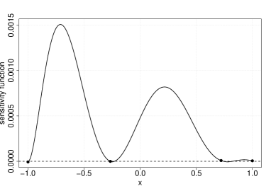
The left part of Figure 2 shows the plots of the sensitivity function on the left-hand side of (3.1) for the design found by Otsu, (2008) (left). We conclude that this design is not optimal for discriminating between the model f1(y,x,θ¯1)subscript𝑓1𝑦𝑥subscript¯𝜃1f_{1}(y,x,\overline{\theta}_{1}) and the class 2subscript2\mathcal{F}_{2}, because the function is positive throughout the design space. The subfigure on the right shows the sensitivity function of the design

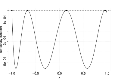
ξ=[1.0000.6700.1420.9590.2530.4280.2470.072],superscript𝜉matrix1.0000.6700.1420.9590.2530.4280.2470.072\displaystyle\xi^{*}=\begin{bmatrix}-1.000&-0.670&0.142&0.959\\ 0.253&0.428&0.247&0.072\end{bmatrix}, (3.6)

which has been found maximizing the criterion provided by Theorem 2.1 and confirms its optimality.
Refer to caption
Refer to caption
Figure 2: The sensitivity functions of two designs for discriminating between models (3.3) and (3.4). The left figure is for the design (3.5) calculated by Otsu, (2008) and the right figure is for the T𝑇T-optimal design (3.6).

The values of the criterion (2.6) for different designs are given by K(a)(ξ~)=3.27779106subscript𝐾𝑎~𝜉3.27779superscript106K_{(a)}(\tilde{\xi})=3.27779*10^{-6} and K(a)(ξ)=0.0005580455subscript𝐾𝑎superscript𝜉0.0005580455K_{(a)}(\xi^{*})=0.0005580455 demonstrating that ξsuperscript𝜉\xi^{*} performs substantially better than ξ~~𝜉\tilde{\xi}; in fact, the efficiency of ξ~~𝜉\tilde{\xi} of the design determined by Otsu, (2008) relative to ξsuperscript𝜉\xi^{*} is approximately 0.0060.0060.006. It turns out that the design in (3.6) is also the T𝑇T-optimal design. In the next section, we prove in Theorem 4.1 that for models (3.3) and (3.4), the semi-parametric optimal design for discriminating between the model f1(y,x,θ¯1)subscript𝑓1𝑦𝑥subscript¯𝜃1f_{1}(y,x,\overline{\theta}_{1}) and the class 2subscript2\mathcal{F}_{2} actually coincides with the T𝑇T-optimal design proposed by Atkinson and Fedorov, 1975a .

4 Analytical results

In this section we investigate relationships between the semi-parametric optimality criteria considered in this paper and the optimality criteria for model discrimination with normal errors [see Atkinson and Fedorov, 1975a and Ucinski and Bogacka, (2005)]. A ”classical” T𝑇T-optimal design, say ξTsuperscriptsubscript𝜉𝑇\xi_{T}^{*}, for discriminating between two models maximizes the criterion

infθ2Θ2𝒳[η1(x,θ¯1)η2(x,θ2)]2ξ(dx)subscriptinfimumsubscript𝜃2subscriptΘ2subscript𝒳superscriptdelimited-[]subscript𝜂1𝑥subscript¯𝜃1subscript𝜂2𝑥subscript𝜃22𝜉𝑑𝑥\inf_{\theta_{2}\in\Theta_{2}}\int_{\cal X}[\eta_{1}(x,\overline{\theta}_{1})-\eta_{2}(x,\theta_{2})]^{2}\xi(dx) (4.1)

among all designs on the design space [see Atkinson and Fedorov, 1975a ], where θ¯1subscript¯𝜃1\overline{\theta}_{1} is fixed. We will presume throughout this section that the infimum in (4.1) is attained at a unique point θ2superscriptsubscript𝜃2\theta_{2}^{*} when ξ=ξT𝜉subscriptsuperscript𝜉𝑇\xi=\xi^{*}_{T}. It follows by similar arguments as given in Wiens, (2009) that under the assumption of a normal distribution, the power of the likelihood ratio test for the hypotheses

H0:η(x)=η1(x,θ¯1)versusH1:η(x)=η2(x,θ2)for some θ2Θ2:subscript𝐻0𝜂𝑥subscript𝜂1𝑥subscript¯𝜃1versussubscript𝐻1:formulae-sequence𝜂𝑥subscript𝜂2𝑥subscript𝜃2for some subscript𝜃2subscriptΘ2H_{0}:\eta(x)=\eta_{1}(x,\overline{\theta}_{1})\leavevmode\nobreak\ \leavevmode\nobreak\ \mbox{versus}\leavevmode\nobreak\ \leavevmode\nobreak\ H_{1}:\eta(x)=\eta_{2}(x,\theta_{2})\leavevmode\nobreak\ \leavevmode\nobreak\ \mbox{for some }\theta_{2}\in\Theta_{2} (4.2)

is an increasing function of the criterion (4.1). The following results give a sufficient condition for the T𝑇T-optimal discriminating design to be a semi-parametric optimal design in the sense of Section 2.

Theorem 4.1

Let the assumptions of the Theorem 2.1 (a) be fulfilled and assume further that the density f1(y,x,θ¯1)subscript𝑓1𝑦𝑥subscript¯𝜃1f_{1}(y,x,\overline{\theta}_{1}) can be represented in the form

f1(y,x,θ¯1)=g(yη1(x,θ¯1))subscript𝑓1𝑦𝑥subscript¯𝜃1𝑔𝑦subscript𝜂1𝑥subscript¯𝜃1f_{1}(y,x,\overline{\theta}_{1})=g(y-\eta_{1}(x,\overline{\theta}_{1})) (4.3)

where g𝑔g is a symmetric density function supported in the interval [a,a]𝑎𝑎[-a,a], i.e. f1subscript𝑓1f_{1} has support [a+η1(x,θ¯1),a+η1(x,θ¯1)]𝑎subscript𝜂1𝑥subscript¯𝜃1𝑎subscript𝜂1𝑥subscript¯𝜃1[-a+\eta_{1}(x,\overline{\theta}_{1}),a+\eta_{1}(x,\overline{\theta}_{1})]. The T𝑇T-optimal discriminating design maximizing the criterion (4.1) is a semi-parametric optimal design for discriminating between the model f1(y,x,θ¯1)subscript𝑓1𝑦𝑥subscript¯𝜃1f_{1}(y,x,\overline{\theta}_{1}) and the class 2subscript2\mathcal{F}_{2}.

A similar result is available for the semi-parametric optimal designs for discriminating between the model f2(y,x,θ2)subscript𝑓2𝑦𝑥subscript𝜃2f_{2}(y,x,\theta_{2}) and the class 1subscript1\mathcal{F}_{1}. For this purpose we consider the situation, where f2(y,x,θ2)subscript𝑓2𝑦𝑥subscript𝜃2f_{2}(y,x,\theta_{2}) is the density of the normal distributions 𝒩(η2(x,θ2),v22(x,θ2))𝒩subscript𝜂2𝑥subscript𝜃2subscriptsuperscript𝑣22𝑥subscript𝜃2{\cal N}(\eta_{2}(x,\theta_{2}),v^{2}_{2}(x,\theta_{2})). If f1(y,x,θ¯1)subscript𝑓1𝑦𝑥subscript¯𝜃1f_{1}(y,x,\overline{\theta}_{1}) is also the density of a 𝒩(η1(x,θ¯1),v22(x,θ2))𝒩subscript𝜂1𝑥subscript¯𝜃1subscriptsuperscript𝑣22𝑥subscript𝜃2{\cal N}(\eta_{1}(x,\overline{\theta}_{1}),v^{2}_{2}(x,\theta_{2})) it can be shown that the power of the likelihood ratio test for the hypotheses (4.2) is an increasing function of the quantity

infθ2Θ2𝒳[η1(x,θ¯1)η2(x,θ2)]2v22(x,θ2)ξ(dx).subscriptinfimumsubscript𝜃2subscriptΘ2subscript𝒳superscriptdelimited-[]subscript𝜂1𝑥subscript¯𝜃1subscript𝜂2𝑥subscript𝜃22subscriptsuperscript𝑣22𝑥subscript𝜃2𝜉𝑑𝑥\displaystyle\inf_{\theta_{2}\in\Theta_{2}}\int_{\cal X}\frac{[\eta_{1}(x,\overline{\theta}_{1})-\eta_{2}(x,\theta_{2})]^{2}}{v^{2}_{2}(x,\theta_{2})}\xi(dx). (4.4)

The maximization of this expression corresponds to the KL-optimal design problem for discriminating between two normal distributions with the same variance as considered by López-Fidalgo et al., (2007). Our following result shows that this design is also optimal for discriminating between the model f2(y,x,θ2)subscript𝑓2𝑦𝑥subscript𝜃2f_{2}(y,x,\theta_{2}) and the class 1subscript1\mathcal{F}_{1}.

Theorem 4.2

Assume that f2(y,x,θ2)subscript𝑓2𝑦𝑥subscript𝜃2f_{2}(y,x,\theta_{2}) is the density of a normal distribution with mean η2(x,θ2)subscript𝜂2𝑥subscript𝜃2\eta_{2}(x,\theta_{2}) and variance v22(x,θ2)superscriptsubscript𝑣22𝑥subscript𝜃2v_{2}^{2}(x,\theta_{2}). The optimal design maximizing (4.4) is a semi-parametric optimal design for discriminating between the model f2(y,x,θ2)subscript𝑓2𝑦𝑥subscript𝜃2f_{2}(y,x,\theta_{2}) and the class 1subscript1\mathcal{F}_{1} and vice versa. Moreover, the best approximation f1(y,x,θ¯1)superscriptsubscript𝑓1𝑦𝑥subscript¯𝜃1f_{1}^{*}(y,x,\overline{\theta}_{1}) is a normal density with mean η1(x,θ¯1)subscript𝜂1𝑥subscript¯𝜃1\eta_{1}(x,\overline{\theta}_{1}) and variance v22(x,θ2)superscriptsubscript𝑣22𝑥subscript𝜃2v_{2}^{2}(x,\theta_{2}).

5 Numerical results

The numerical construction of semi-parameteric optimal discrimination designs is a very challenging problem. In this section we describe techniques for finding semi-parametric optimal designs and illustrate our approach in two examples. It follows from the results of Section 2 that the first step in the determination of the optimal designs consists in an efficient solution of the equations (2.9) and (2.15). In a second step any numerical method for the determination of KL-optimal discrimination designs can be adapted to the minimax problems obtained from Theorem 2.1 as the representations (2.11) and (2.13) have a similar structure as the KL-optimality criteria considered in López-Fidalgo et al., (2007). Even the second step defines a very challenging problem and some recent results and algorithms for KL-optimality criteria can be found in (Stegmaier et al., , 2013), Braess and Dette, (2013); Dette et al., (2015) and Dette et al., 2016a . As the focus in this paper is on the new semi-parametric design criteria we concentrate on the first step in the following discussion. For the second step we used an adaptation of the first-order algorithm of Atkinson and Fedorov, 1975a , because it can easily be implemented.

Let δ𝛿\delta be a user-selected positive constant. For finding the numerical solution of the equation (2.9) we propose the following algorithm:

  • if η1(x,θ¯1)=η2(x,θ2)subscript𝜂1𝑥subscript¯𝜃1subscript𝜂2𝑥subscript𝜃2\eta_{1}(x,\overline{\theta}_{1})=\eta_{2}(x,\theta_{2}), set λ=0𝜆0\lambda=0;

  • if η1(x,θ¯1)<η2(x,θ2)subscript𝜂1𝑥subscript¯𝜃1subscript𝜂2𝑥subscript𝜃2\eta_{1}(x,\overline{\theta}_{1})<\eta_{2}(x,\theta_{2}), choose a solution in the interval Λ=[1/(yx,maxη2(x,θ2)),δ]superscriptΛ1subscript𝑦𝑥subscript𝜂2𝑥subscript𝜃2𝛿{{\Lambda}^{-}=[-1/(y_{x,\max}-\eta_{2}(x,\theta_{2})),-\delta]};

  • if η1(x,θ¯1)>η2(x,θ2)subscript𝜂1𝑥subscript¯𝜃1subscript𝜂2𝑥subscript𝜃2\eta_{1}(x,\overline{\theta}_{1})>\eta_{2}(x,\theta_{2}), choose a solution in the interval Λ+=[δ,1/(yx,minη2(x,θ2))]superscriptΛ𝛿1subscript𝑦𝑥subscript𝜂2𝑥subscript𝜃2{{\Lambda}^{+}=[\delta,-1/(y_{x,\min}-\eta_{2}(x,\theta_{2}))]}.

Similarly, the solution of (2.15) can be obtained as follows. We search for λ>0𝜆0\lambda>0 if η1(x,θ¯1)<η2(x,θ2)subscript𝜂1𝑥subscript¯𝜃1subscript𝜂2𝑥subscript𝜃2\eta_{1}(x,\overline{\theta}_{1})<\eta_{2}(x,\theta_{2}) so that λ𝜆\lambda shifts the predefined density f2(y,x,θ2)subscript𝑓2𝑦𝑥subscript𝜃2f_{2}(y,x,\theta_{2}) to the left and, search for λ<0𝜆0\lambda<0 if η1(x,θ¯1)>η2(x,θ2)subscript𝜂1𝑥subscript¯𝜃1subscript𝜂2𝑥subscript𝜃2\eta_{1}(x,\overline{\theta}_{1})>\eta_{2}(x,\theta_{2}). Let β𝛽\beta be a large user-selected positive constant, let δ𝛿\delta be a small positive constant and assume that the solution of (2.15) is in [β,+β]𝛽𝛽[-\beta,+\beta]. We note that

μ(λ)f2(y,x,θ2)exp(λy)>0,λ[β,+β],formulae-sequencesuperscript𝜇𝜆subscript𝑓2𝑦𝑥subscript𝜃2𝜆𝑦0for-all𝜆𝛽𝛽\displaystyle\mu^{\prime}(\lambda)f_{2}(y,x,\theta_{2})\exp(-\lambda y)>0,\;\forall\lambda\in[-\beta,+\beta],

for all y𝒮f2,θ2,x,𝑦subscript𝒮subscript𝑓2subscript𝜃2𝑥y\in{\cal S}_{f_{2},\theta_{2},x}, where μ(λ)superscript𝜇𝜆\mu^{\prime}(\lambda) is defined in (2.14). We suggest the following algorithm for finding a numeral solution of (2.15):

  • if η1(x,θ¯1)=η2(x,θ2)subscript𝜂1𝑥subscript¯𝜃1subscript𝜂2𝑥subscript𝜃2\eta_{1}(x,\overline{\theta}_{1})=\eta_{2}(x,\theta_{2}), set λ=0𝜆0\lambda=0;

  • if η1(x,θ¯1)<η2(x,θ2)subscript𝜂1𝑥subscript¯𝜃1subscript𝜂2𝑥subscript𝜃2\eta_{1}(x,\overline{\theta}_{1})<\eta_{2}(x,\theta_{2}), choose a solution in the interval Λ+=[+δ,+β]superscriptΛ𝛿𝛽{\Lambda}^{+}=[+\delta,+\beta];

  • if η1(x,θ¯1)>η2(x,θ2)subscript𝜂1𝑥subscript¯𝜃1subscript𝜂2𝑥subscript𝜃2\eta_{1}(x,\overline{\theta}_{1})>\eta_{2}(x,\theta_{2}), choose a solution in the interval Λ=[β,δ]superscriptΛ𝛽𝛿\Lambda^{-}=[-\beta,-\delta].

We now present two examples, where the T𝑇T-optimal and semi-parametric KLlimit-from𝐾𝐿KL-optimal designs are determined numerically and shown to be different. To be precise, consider the optimal design problem from  López-Fidalgo et al., (2007), where they were interested to discriminate between the two models:

η1(x,θ1)subscript𝜂1𝑥subscript𝜃1\displaystyle\eta_{1}(x,\theta_{1}) =θ1,1x+θ1,2xx+θ1,3,absentsubscript𝜃11𝑥subscript𝜃12𝑥𝑥subscript𝜃13\displaystyle=\theta_{1,1}x+\frac{\theta_{1,2}x}{x+\theta_{1,3}}, (5.1)
η2(x,θ2)subscript𝜂2𝑥subscript𝜃2\displaystyle\eta_{2}(x,\theta_{2}) =θ2,1xx+θ2,2.absentsubscript𝜃21𝑥𝑥subscript𝜃22\displaystyle=\frac{\theta_{2,1}x}{x+\theta_{2,2}}. (5.2)

The design space for both models is the interval [0.1,5]0.15[0.1,5] and we assume that the first model has fixed parameters θ¯1=(1,1,1)subscript¯𝜃1111\overline{\theta}_{1}=(1,1,1). We construct three different types of optimal discrimination designs for this problem: a T𝑇T-optimal design, a KL-optimal design for lognormal errors (with fixed variances v12(x,θ¯1)=v22(x,θ2)=0.1subscriptsuperscript𝑣21𝑥subscript¯𝜃1subscriptsuperscript𝑣22𝑥subscript𝜃20.1v^{2}_{1}(x,\overline{\theta}_{1})=v^{2}_{2}(x,\theta_{2})=0.1) and a semi-parametric KL-optimal design (case a)) for a mildly truncated lognormal density f1(y,x,θ¯1)subscript𝑓1𝑦𝑥subscript¯𝜃1f_{1}(y,x,\overline{\theta}_{1}) with location and scale parameters, respectively, given by

μ1(x,θ¯1)subscript𝜇1𝑥subscript¯𝜃1\displaystyle\mu_{1}(x,\overline{\theta}_{1}) =log[η1(x,θ¯1)]12log[1+v12(x,θ¯1)/η12(x,θ¯1)],absentsubscript𝜂1𝑥subscript¯𝜃1121subscriptsuperscript𝑣21𝑥subscript¯𝜃1superscriptsubscript𝜂12𝑥subscript¯𝜃1\displaystyle=\log\left[\eta_{1}(x,\overline{\theta}_{1})\right]-\frac{1}{2}\log\left[1+v^{2}_{1}(x,\overline{\theta}_{1})/\eta_{1}^{2}(x,\overline{\theta}_{1})\right],
σ12(x,θ¯1)subscriptsuperscript𝜎21𝑥subscript¯𝜃1\displaystyle\sigma^{2}_{1}(x,\overline{\theta}_{1}) =log[1+v12(x,θ¯1)/η12(x,θ¯1)].absent1subscriptsuperscript𝑣21𝑥subscript¯𝜃1superscriptsubscript𝜂12𝑥subscript¯𝜃1\displaystyle=\log\left[1+v^{2}_{1}(x,\overline{\theta}_{1})/\eta_{1}^{2}(x,\overline{\theta}_{1})\right].

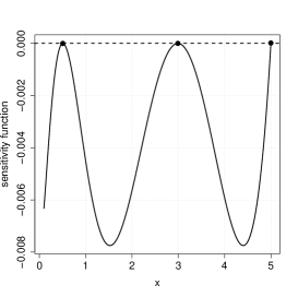
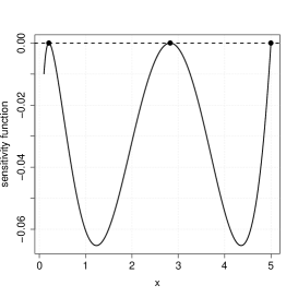
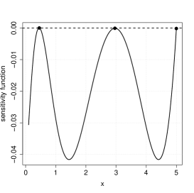
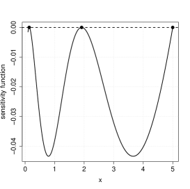
The range for this density is the interval from Q(0.0001,x,θ¯1)𝑄0.0001𝑥subscript¯𝜃1Q(0.0001,x,\overline{\theta}_{1}) to Q(0.9999,x,θ¯1)𝑄0.9999𝑥subscript¯𝜃1Q(0.9999,x,\overline{\theta}_{1}), where Q(p,x,θ¯1)𝑄𝑝𝑥subscript¯𝜃1Q(p,x,\overline{\theta}_{1}) is quantile function of ordinary lognormal density with mean η1(x,θ¯1)subscript𝜂1𝑥subscript¯𝜃1\eta_{1}(x,\overline{\theta}_{1}) and variance v12(x,θ¯1)=0.1superscriptsubscript𝑣12𝑥subscript¯𝜃10.1v_{1}^{2}(x,\overline{\theta}_{1})=0.1. We note that because of mild truncation η1(x,θ¯1)subscript𝜂1𝑥subscript¯𝜃1\eta_{1}(x,\overline{\theta}_{1}) does not correspond exactly to the mean of f1(y,x,θ¯1)subscript𝑓1𝑦𝑥subscript¯𝜃1f_{1}(y,x,\overline{\theta}_{1}) but is very close to it. The optimal discrimination designs under the three different criteria are displayed in Table 1, where we also show the “optimal” parameter θ2superscriptsubscript𝜃2\theta_{2}^{*} of the second model corresponding to the minimal value with respect to the parameter θ2subscript𝜃2\theta_{2}. We observe substantial differences between the T𝑇T, KL𝐾𝐿KL- and semi-parametric KL𝐾𝐿KL-optimal discrimination (SKL) designs. Figure 3 displays the sensitivity functions of the three designs and confirms the optimality of each of the designs.

Table 2 displays the efficiencies of T𝑇T, KL𝐾𝐿KL- and semi-parametric KL𝐾𝐿KL-optimal discrimination (SKL) designs with respect to the different criteria. For example, the value 0.2470.2470.247 in the first row is the efficiency of the KL𝐾𝐿KL-optimal design with respect to the T𝑇T-optimality criterion. We observe that the T𝑇T- and KL𝐾𝐿KL- optimal discrimination design are not very robust under a variation of the criteria, where the KL𝐾𝐿KL-optimal discrimination design has slight advantages. On the other hand, the semi-parametric KL𝐾𝐿KL-optimal discrimination design yields moderate efficiencies (about 75%percent7575\%) with respect to the T𝑇T- and KL𝐾𝐿KL-optimality criterion. Figure 4 shows the plots of the functions f1(y,xi,θ¯1)subscript𝑓1𝑦superscriptsubscript𝑥𝑖subscript¯𝜃1f_{1}(y,x_{i}^{*},\overline{\theta}_{1}) and f2(y,xi,θ2)superscriptsubscript𝑓2𝑦subscriptsuperscript𝑥𝑖superscriptsubscript𝜃2f_{2}^{*}(y,x^{*}_{i},\theta_{2}^{*}) for the support points xisuperscriptsubscript𝑥𝑖x_{i}^{*}, i=1,2,3𝑖123i=1,2,3 of SKL𝑆𝐾𝐿SKL-optimal design. Above each figure the values η1(xi,θ¯1)subscript𝜂1subscript𝑥𝑖subscript¯𝜃1\eta_{1}(x_{i},\overline{\theta}_{1}), η2(xi,θ2)subscript𝜂2subscript𝑥𝑖superscriptsubscript𝜃2\eta_{2}(x_{i},\theta_{2}^{*}) and λ¯(xi,θ¯1,θ2)¯𝜆superscriptsubscript𝑥𝑖subscript¯𝜃1superscriptsubscript𝜃2\overline{\lambda}(x_{i}^{*},\overline{\theta}_{1},\theta_{2}^{*}), the solution of (2.9), are presented. We note that the densities f1subscript𝑓1f_{1} and f2superscriptsubscript𝑓2f_{2}^{*} depend on the parameters θ¯1subscript¯𝜃1\overline{\theta}_{1} and θ2superscriptsubscript𝜃2\theta_{2}^{*} only through η1(x,θ¯1)subscript𝜂1𝑥subscript¯𝜃1\eta_{1}(x,\overline{\theta}_{1}) and η2(x,θ2)subscript𝜂2𝑥subscriptsuperscript𝜃2\eta_{2}(x,\theta^{*}_{2}).

Design type ξsuperscript𝜉\xi^{*} θ2superscriptsubscript𝜃2\theta_{2}^{*}
T𝑇T-optimal 0.5082.9925.0000.5800.2980.122matrix0.5082.9925.0000.5800.2980.122\begin{matrix}0.508&2.992&5.000\\ 0.580&0.298&0.122\end{matrix} (22.564,14.637)22.56414.637(22.564,14.637)
KL𝐾𝐿KL-optimal 0.2062.8265.0000.5740.3080.118matrix0.2062.8265.0000.5740.3080.118\begin{matrix}0.206&2.826&5.000\\ 0.574&0.308&0.118\end{matrix} (20.552,12.962)20.55212.962(20.552,12.962)
SKL𝑆𝐾𝐿SKL-optimal 0.4542.9615.0000.5310.3440.125matrix0.4542.9615.0000.5310.3440.125\begin{matrix}0.454&2.961&5.000\\ 0.531&0.344&0.125\end{matrix} (22.045,14.197)22.04514.197(22.045,14.197)
Table 1: T𝑇T, KL𝐾𝐿KL- and semi-parametric KL𝐾𝐿KL-optimal discrimination (SKL) designs for discriminating between models (5.1) and (5.2).
Refer to caption
(a) T𝑇T-optimal
Refer to caption
(b) KL𝐾𝐿KL-optimal
Refer to caption
(c) SKL𝑆𝐾𝐿SKL-optimal
Figure 3: The sensitivity functions of the T𝑇T-, KL𝐾𝐿KL- and semi-parametric KL𝐾𝐿KL-optimal discrimination (SKL) designs in Table 1.
K(ξ)ξ𝐾𝜉𝜉K(\xi)\setminus\xi T𝑇T KL𝐾𝐿KL SKL𝑆𝐾𝐿SKL
T𝑇T 1 0.247 0.741
KL𝐾𝐿KL 0.653 1 0.787
SKL𝑆𝐾𝐿SKL 0.55 0.397 1
Table 2: Efficiencies of the T𝑇T, KL𝐾𝐿KL- and semi-parametric KL𝐾𝐿KL-optimal discrimination (SKL) designs for the models (5.1) and (5.2) under different optimality criteria.
Refer to caption
Refer to caption
Refer to caption
Figure 4: The density f1(y,xi,θ¯1)subscript𝑓1𝑦superscriptsubscript𝑥𝑖subscript¯𝜃1f_{1}(y,x_{i}^{*},\overline{\theta}_{1}) of a truncated lognormal distribution (solid line) on the interval [Q(0.0001,xi,θ¯1),Q(0.9999,xi,θ¯1)]𝑄0.0001superscriptsubscript𝑥𝑖subscript¯𝜃1𝑄0.9999superscriptsubscript𝑥𝑖subscript¯𝜃1[Q(0.0001,x_{i}^{*},\overline{\theta}_{1}),Q(0.9999,x_{i}^{*},\overline{\theta}_{1})] and the corresponding “optimal” density f2(y,xi,θ2)superscriptsubscript𝑓2𝑦superscriptsubscript𝑥𝑖superscriptsubscript𝜃2f_{2}^{*}(y,x_{i}^{*},\theta_{2}^{*}), defined by (2.12), for the support points xisuperscriptsubscript𝑥𝑖x_{i}^{*}, i=1,2,3𝑖123i=1,2,3 of SKL-optimal design and parameter values θ2superscriptsubscript𝜃2\theta_{2}^{*} from Table 1.

As a second example we now consider a similar problem with a different function η1(x,θ1)subscript𝜂1𝑥subscript𝜃1\eta_{1}(x,\theta_{1}) (Wiens, , 2009). The two models of interest are

η1(x,θ1)subscript𝜂1𝑥subscript𝜃1\displaystyle\eta_{1}(x,\theta_{1}) =\displaystyle= θ1,1{1exp(θ1,2x)},subscript𝜃111subscript𝜃12𝑥\displaystyle\theta_{1,1}\big{\{}1-\exp(-\theta_{1,2}x)\big{\}}, (5.3)
η2(x,θ2)subscript𝜂2𝑥subscript𝜃2\displaystyle\eta_{2}(x,\theta_{2}) =\displaystyle= θ2,1xθ2,2+x,subscript𝜃21𝑥subscript𝜃22𝑥\displaystyle\frac{\theta_{2,1}x}{\theta_{2,2}+x}, (5.4)

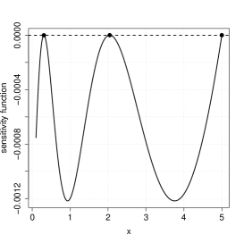
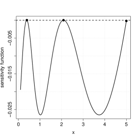
where the design space is given by the interval 𝒳=[0.1,5]𝒳0.15{\cal X}=[0.1,5]. Here we fix the parameters of the model (5.3) as θ¯1=(1,1)subscript¯𝜃111\overline{\theta}_{1}=(1,1) and determine the T𝑇T-optimal, KL𝐾𝐿KL-optimal (for lognormal errors) and a semi-parametric KL𝐾𝐿KL-optimal design (case a)) for mildly truncated lognormal errors. The error variances for the KL𝐾𝐿KL-optimal discrimination design are v12(x,θ¯1)=v22(x,θ2)=0.02superscriptsubscript𝑣12𝑥subscript¯𝜃1superscriptsubscript𝑣22𝑥subscript𝜃20.02v_{1}^{2}(x,\overline{\theta}_{1})=v_{2}^{2}(x,\theta_{2})=0.02 and for the semi-parametric KL𝐾𝐿KL-optimal the variance is v12(x,θ¯1)=0.02superscriptsubscript𝑣12𝑥subscript¯𝜃10.02v_{1}^{2}(x,\overline{\theta}_{1})=0.02. The optimal designs with respect to the different criteria are presented in Table 3, where we also show the corresponding parameter θ2superscriptsubscript𝜃2\theta_{2}^{*} of the second model corresponding to the minimal value with respect to the parameter θ2subscript𝜃2\theta_{2}. We observe again substantial differences between the optimal discrimination designs with respect to the different criteria, and a comparison of the efficiencies of the optimal designs with respect ot the different criteria in Table 4 shows a similar picture as in the first example. Figure 5 displays the sensitivity functions of the T𝑇T-, KL𝐾𝐿KL- and semi-parametric KL𝐾𝐿KL-optimal discrimination designs and the three subplots confirm optimality of the three three-point designs. Figure 6 shows the plots of the functions f1(y,xi,θ¯1)subscript𝑓1𝑦superscriptsubscript𝑥𝑖subscript¯𝜃1f_{1}(y,x_{i}^{*},\overline{\theta}_{1}) and f2(y,xi,θ2)superscriptsubscript𝑓2𝑦subscriptsuperscript𝑥𝑖superscriptsubscript𝜃2f_{2}^{*}(y,x^{*}_{i},\theta_{2}^{*}) for the support points xisuperscriptsubscript𝑥𝑖x_{i}^{*}, i=1,2,3𝑖123i=1,2,3 of SKL𝑆𝐾𝐿SKL-optimal design from Table 3, the legend above each plot has the same meaning as before.

Design type ξsuperscript𝜉\xi^{*} θ2superscriptsubscript𝜃2\theta_{2}^{*}
T𝑇T-optimal 0.3082.0445.0000.3160.4280.256matrix0.3082.0445.0000.3160.4280.256\begin{matrix}0.308&2.044&5.000\\ 0.316&0.428&0.256\end{matrix} (1.223,0.948)1.2230.948(1.223,0.948)
KL𝐾𝐿KL-optimal 0.1401.9165.0000.3330.4020.465matrix0.1401.9165.0000.3330.4020.465\begin{matrix}0.140&1.916&5.000\\ 0.333&0.402&0.465\end{matrix} (1.242,1.006)1.2421.006(1.242,1.006)
SKL𝑆𝐾𝐿SKL-optimal 0.3952.0905.0000.3960.3550.249matrix0.3952.0905.0000.3960.3550.249\begin{matrix}0.395&2.090&5.000\\ 0.396&0.355&0.249\end{matrix} (1.216,0.920)1.2160.920(1.216,0.920)
Table 3: T𝑇T, KL𝐾𝐿KL- and semi-parametric KL𝐾𝐿KL-optimal discrimination (SKL) designs for discriminating between the models (5.3) and (5.4).
K(ξ)ξ𝐾𝜉𝜉K(\xi)\setminus\xi T𝑇T KL𝐾𝐿KL SKL𝑆𝐾𝐿SKL
T𝑇T 1 0.360 0.663
KL𝐾𝐿KL 0.835 1 0.655
SKL𝑆𝐾𝐿SKL 0.407 0.361 1
Table 4: Efficiencies of the T𝑇T, KL𝐾𝐿KL- and semi-parametric KL𝐾𝐿KL-optimal discrimination (SKL) designs for the models (5.3) and (5.4) under various optimality criteria.
Refer to caption
(a) T𝑇T-optimal
Refer to caption
(b) KL𝐾𝐿KL-optimal
Refer to caption
(c) SKL𝑆𝐾𝐿SKL-optimal
Figure 5: The sensitivity functions of the T𝑇T-, KL𝐾𝐿KL- and semi-parametric KL𝐾𝐿KL-optimal discrimination (SKL) designs in Table 3.
Refer to caption
Refer to caption
Refer to caption
Figure 6: The density f1(y,xi,θ¯1)subscript𝑓1𝑦superscriptsubscript𝑥𝑖subscript¯𝜃1f_{1}(y,x_{i}^{*},\overline{\theta}_{1}) of a truncated lognormal distribution (solid line) and the “optimal” density f2(y,xi,θ2)superscriptsubscript𝑓2𝑦superscriptsubscript𝑥𝑖superscriptsubscript𝜃2f_{2}^{*}(y,x_{i}^{*},\theta_{2}^{*}) for the support points xisuperscriptsubscript𝑥𝑖x_{i}^{*}, i=1,2,3𝑖123i=1,2,3 of SKL-optimal design and corresponding “optimal” parameter values θ2superscriptsubscript𝜃2\theta_{2}^{*} from Table 3.

6 Proofs

Proof of Theorem 2.1: We only prove the first part of the proposition. The second statement follows by similar arguments which are omitted for the sake of brevity. We first introduce the following temporary notation

f1(y,x,θ¯1)=f1(y),f2(y,x,θ2)=f2(y),η1(x,θ¯1)=η1,η2(x,θ2)=η2,formulae-sequencesubscript𝑓1𝑦𝑥subscript¯𝜃1subscript𝑓1𝑦formulae-sequencesubscript𝑓2𝑦𝑥subscript𝜃2subscript𝑓2𝑦formulae-sequencesubscript𝜂1𝑥subscript¯𝜃1subscript𝜂1subscript𝜂2𝑥subscript𝜃2subscript𝜂2\displaystyle f_{1}(y,x,\overline{\theta}_{1})=f_{1}(y),\;f_{2}(y,x,\theta_{2})=f_{2}(y),\;\eta_{1}(x,\overline{\theta}_{1})=\eta_{1},\;\eta_{2}(x,\theta_{2})=\eta_{2}, (6.1)

and note that from (2.6), we wish to minimize

I1,2(x,f1,f2,θ1,θ2)=log{f1(y)f2(y)}f1(y)𝑑ysubscript𝐼12𝑥subscript𝑓1subscript𝑓2subscript𝜃1subscript𝜃2subscript𝑓1𝑦subscript𝑓2𝑦subscript𝑓1𝑦differential-d𝑦\displaystyle I_{1,2}(x,f_{1},f_{2},\theta_{1},\theta_{2})=\int\log{\left\{\frac{f_{1}(y)}{f_{2}(y)}\right\}}f_{1}(y)dy

with constraints

f2(y)𝑑y=1,andyf2(y)𝑑y=η2.formulae-sequencesubscript𝑓2𝑦differential-d𝑦1and𝑦subscript𝑓2𝑦differential-d𝑦subscript𝜂2\displaystyle\int f_{2}(y)dy=1,\ \leavevmode\nobreak\ \text{and}\leavevmode\nobreak\ \int yf_{2}(y)dy=\eta_{2}. (6.2)

Consequently, with the notation

H=log{f1(y)f2(y)}f1(y)+μf2(y)+λyf2(y),𝐻subscript𝑓1𝑦subscript𝑓2𝑦subscript𝑓1𝑦𝜇subscript𝑓2𝑦𝜆𝑦subscript𝑓2𝑦\displaystyle H=\log{\left\{\frac{f_{1}(y)}{f_{2}(y)}\right\}}f_{1}(y)+\mu f_{2}(y)+\lambda yf_{2}(y)\leavevmode\nobreak\ ,

we obtain the Euler-Lagrange equation

Hf2=f1(y)f2(y)+μ+λy=0𝐻subscript𝑓2subscript𝑓1𝑦subscript𝑓2𝑦𝜇𝜆𝑦0\displaystyle\frac{\partial H}{\partial f_{2}}=-\frac{f_{1}(y)}{f_{2}(y)}+\mu+\lambda y=0

and the relation

f2(y)=f1(y)μ+λy.subscript𝑓2𝑦subscript𝑓1𝑦𝜇𝜆𝑦\displaystyle f_{2}(y)=\frac{f_{1}(y)}{\mu+\lambda y}. (6.3)

We may assume without loss of generality that λ0𝜆0\lambda\neq 0 ; otherwise, we have μ=1𝜇1\mu=1 and f2(y)=f1(y)subscript𝑓2𝑦subscript𝑓1𝑦f_{2}(y)=f_{1}(y). From the condition (6.2) and (6.3) we obtain

η2subscript𝜂2\displaystyle\eta_{2} =yf2(y)𝑑y=yμ+λyf1(y)𝑑yabsent𝑦subscript𝑓2𝑦differential-d𝑦𝑦𝜇𝜆𝑦subscript𝑓1𝑦differential-d𝑦\displaystyle=\int yf_{2}(y)dy=\int\frac{y}{\mu+\lambda y}f_{1}(y)dy
=1λμ+λyμ+λyf1(y)𝑑yμλ1μ+λyf1(y)𝑑y=1λμλ.absent1𝜆𝜇𝜆𝑦𝜇𝜆𝑦subscript𝑓1𝑦differential-d𝑦𝜇𝜆1𝜇𝜆𝑦subscript𝑓1𝑦differential-d𝑦1𝜆𝜇𝜆\displaystyle=\frac{1}{\lambda}\int\frac{\mu+\lambda y}{\mu+\lambda y}f_{1}(y)dy-\frac{\mu}{\lambda}\int\frac{1}{\mu+\lambda y}f_{1}(y)dy=\frac{1}{\lambda}-\frac{\mu}{\lambda}.

Hence we have μ=1η2λ𝜇1subscript𝜂2𝜆\mu=1-\eta_{2}\lambda and

f2(y)=f1(y)1+λ(yη2).subscript𝑓2𝑦subscript𝑓1𝑦1𝜆𝑦subscript𝜂2\displaystyle f_{2}(y)=\frac{f_{1}(y)}{1+\lambda(y-\eta_{2})}\leavevmode\nobreak\ .

Substituting the new expression for f2(y)subscript𝑓2𝑦f_{2}(y) into the remaining condition gives

f1(y)1+λ(yη2)𝑑y=1.subscript𝑓1𝑦1𝜆𝑦subscript𝜂2differential-d𝑦1\displaystyle\int\frac{f_{1}(y)}{1+\lambda(y-\eta_{2})}dy=1. (6.4)

By the assumption in the theorem, equation (6.4) has a unique solution in the interval (2.10) and the inequality

1+λ¯(yη2)>01¯𝜆𝑦subscript𝜂20\displaystyle 1+\overline{\lambda}(y-\eta_{2})>0

holds for all y𝒮f1,θ¯1,x𝑦subscript𝒮subscript𝑓1subscript¯𝜃1𝑥y\in\mathcal{S}_{f_{1},\overline{\theta}_{1},x}, where λ¯¯𝜆\overline{\lambda} solves (6.4). This implies that f2subscript𝑓2f_{2} is a density. \Box


Proof of Lemma 2.1: We again use the notation in (6.1). Let λ¯¯𝜆\overline{\lambda} be the solution of equation (2.9) and f2superscriptsubscript𝑓2f_{2}^{*} be the “optimal” density defined by (2.12), then

η1η2subscript𝜂1subscript𝜂2\displaystyle\eta_{1}-\eta_{2} =yf1(y)𝑑yyf2(y)𝑑y=yf1(y){111+λ¯(yη2)}𝑑yabsent𝑦subscript𝑓1𝑦differential-d𝑦𝑦superscriptsubscript𝑓2𝑦differential-d𝑦𝑦subscript𝑓1𝑦111¯𝜆𝑦subscript𝜂2differential-d𝑦\displaystyle=\int yf_{1}(y)dy-\int yf_{2}^{*}(y)dy=\int yf_{1}(y)\left\{1-\frac{1}{1+\overline{\lambda}(y-\eta_{2})}\right\}dy
=yf1(y)λ¯(yη2)1+λ¯(yη2)𝑑y=λ¯y(yη2)f2(y)𝑑yabsent𝑦subscript𝑓1𝑦¯𝜆𝑦subscript𝜂21¯𝜆𝑦subscript𝜂2differential-d𝑦¯𝜆𝑦𝑦subscript𝜂2subscript𝑓2𝑦differential-d𝑦\displaystyle=\int yf_{1}(y)\frac{\overline{\lambda}(y-\eta_{2})}{1+\overline{\lambda}(y-\eta_{2})}dy=\overline{\lambda}\int y(y-\eta_{2})f_{2}(y)dy
=λ¯(yη2)2f2(y)𝑑y+(yη2η22)f2(y)𝑑y=λ¯v22,absent¯𝜆superscript𝑦subscript𝜂22subscript𝑓2𝑦differential-d𝑦𝑦subscript𝜂2superscriptsubscript𝜂22subscript𝑓2𝑦differential-d𝑦¯𝜆superscriptsubscript𝑣22\displaystyle=\overline{\lambda}\int(y-\eta_{2})^{2}f_{2}(y)dy+\int(y\eta_{2}-\eta_{2}^{2})f_{2}(y)dy=\overline{\lambda}v_{2}^{2},

where v22>0superscriptsubscript𝑣220v_{2}^{2}>0 is the variance of f2(y)subscript𝑓2𝑦f_{2}(y), and the last equality follows from the fact that

yf2(y)𝑑y=η2.𝑦subscript𝑓2𝑦differential-d𝑦subscript𝜂2\int yf_{2}(y)dy=\eta_{2}.

\square


Proof of Theorem 3.1: Again we only prove part (a). Part (b) follows by similar arguments. Roughly speaking, the equivalence theorem is a consequence of the equivalence theorem for KL-optimal designs using the specific density for the second model

f2(y,x,θ2)=f1(y,x,θ¯1)1+λ(yη2(x,θ2))superscriptsubscript𝑓2𝑦𝑥subscript𝜃2subscript𝑓1𝑦𝑥subscript¯𝜃11𝜆𝑦subscript𝜂2𝑥subscript𝜃2f_{2}^{*}(y,x,\theta_{2})=\frac{f_{1}(y,x,{\overline{\theta}_{1}})}{1+\lambda(y-\eta_{2}(x,\theta_{2}))}

in the KL-criterion. More specifically, the criterion K(a)(ξ,θ¯1)subscript𝐾𝑎𝜉subscript¯𝜃1K_{(a)}(\xi,{\overline{\theta}_{1}}) is concave and to obtain the equivalence theorem, we calculate the directional derivative as follows:

K(a)([1α]ξ+αξx,θ¯1)α=infθ2Θ2𝒳I1,2(x,f1,f2,θ¯1,θ2)([1α]ξ+αξx)(dx)α,subscript𝐾𝑎delimited-[]1𝛼𝜉𝛼subscript𝜉superscript𝑥subscript¯𝜃1𝛼subscriptinfimumsubscript𝜃2subscriptΘ2subscript𝒳subscript𝐼12𝑥subscript𝑓1subscript𝑓2subscript¯𝜃1subscript𝜃2delimited-[]1𝛼𝜉𝛼subscript𝜉superscript𝑥𝑑𝑥𝛼\displaystyle\frac{\partial K_{(a)}([1-\alpha]\xi+\alpha\xi_{x^{*}},{\overline{\theta}_{1}})}{\partial\alpha}=\frac{\partial\inf_{\theta_{2}\in\Theta_{2}}\int_{\mathcal{X}}I_{1,2}(x,f_{1},f_{2},{\overline{\theta}_{1}},\theta_{2})([1-\alpha]\xi+\alpha\xi_{x^{*}})(dx)}{\partial\alpha},

where ξxsubscript𝜉superscript𝑥\xi_{x^{*}} is the Dirac measure at xsuperscript𝑥x^{*}. By theorem in Pshenichnyi, (1971) on page 75, and the assumptions in our theorem, we have

K(a)([1α]ξ+αξx,θ¯1)αsubscript𝐾𝑎delimited-[]1𝛼𝜉𝛼subscript𝜉superscript𝑥subscript¯𝜃1𝛼\displaystyle\frac{\partial K_{(a)}([1-\alpha]\xi+\alpha\xi_{x^{*}},{\overline{\theta}_{1}})}{\partial\alpha} =𝒳I1,2(x,f1,f2,θ¯1,θ^2)ξx(dx)infθ2Θ2𝒳I1,2(x,f1,f2,θ¯1,θ2)ξ(dx)absentsubscript𝒳subscript𝐼12𝑥subscript𝑓1subscript𝑓2subscript¯𝜃1subscript^𝜃2subscript𝜉superscript𝑥𝑑𝑥subscriptinfimumsubscript𝜃2subscriptΘ2subscript𝒳subscript𝐼12𝑥subscript𝑓1subscript𝑓2subscript¯𝜃1subscript𝜃2𝜉𝑑𝑥\displaystyle=\int_{\mathcal{X}}I_{1,2}(x,f_{1},f_{2},{\overline{\theta}_{1}},\widehat{\theta}_{2})\xi_{x^{*}}(dx)-\inf_{\theta_{2}\in\Theta_{2}}\int_{\mathcal{X}}I_{1,2}(x,f_{1},f_{2},{\overline{\theta}_{1}},\theta_{2})\xi(dx)
=I1,2(x,f1,f2,θ¯1,θ^2)K(a)(ξ,θ¯1),absentsubscript𝐼12superscript𝑥subscript𝑓1subscript𝑓2subscript¯𝜃1subscript^𝜃2subscript𝐾𝑎𝜉subscript¯𝜃1\displaystyle=I_{1,2}(x^{*},f_{1},f_{2},{\overline{\theta}_{1}},\widehat{\theta}_{2})-K_{(a)}(\xi,\overline{\theta}_{1}),

where

θ^2=arginfθ2Θ2𝒳I1,2(x,f1,f2,θ¯1,θ2)ξ(dx).subscript^𝜃2subscriptarginfsubscript𝜃2subscriptΘ2subscript𝒳subscript𝐼12𝑥subscript𝑓1subscript𝑓2subscript¯𝜃1subscript𝜃2𝜉𝑑𝑥\displaystyle\widehat{\theta}_{2}=\operatorname*{arg\,inf}_{\theta_{2}\in\Theta_{2}}\int_{\mathcal{X}}I_{1,2}(x,f_{1},f_{2},{\overline{\theta}_{1}},\theta_{2})\xi(dx).

The design ξsuperscript𝜉\xi^{*} is optimal if and only if the inequality

K(a)([1α]ξ+αξx,θ¯1)α0.subscript𝐾𝑎delimited-[]1𝛼superscript𝜉𝛼subscript𝜉𝑥subscript¯𝜃1𝛼0\frac{\partial K_{(a)}([1-\alpha]\xi^{*}+\alpha\xi_{x},{\overline{\theta}_{1}})}{\partial\alpha}\leq 0.

holds for every x𝒳𝑥𝒳x\in\mathcal{X}, which means that we can not improve the concave functional K(a)(ξ,θ¯1)subscript𝐾𝑎superscript𝜉subscript¯𝜃1K_{(a)}(\xi^{*},{\overline{\theta}_{1}}) by moving in any direction from ξsuperscript𝜉\xi^{*}. \square


Proof of Theorem 4.1: With the notations (6.1) consider the function

F(η1,η2,λ)𝐹subscript𝜂1subscript𝜂2𝜆\displaystyle F(\eta_{1},\eta_{2},\lambda) =a+η1a+η1log{1+λ(yη2)}f1(y)𝑑yabsentsuperscriptsubscript𝑎subscript𝜂1𝑎subscript𝜂11𝜆𝑦subscript𝜂2subscript𝑓1𝑦differential-d𝑦\displaystyle=\int_{-a+\eta_{1}}^{a+\eta_{1}}\log\left\{1+\lambda(y-\eta_{2})\right\}f_{1}(y)dy
=aalog{1+λ(tΔη)}g(t)dt=:F(Δη,λ),\displaystyle=\int_{-a}^{a}\log\left\{1+\lambda(t-\Delta_{\eta})\right\}g(t)dt=:F(\Delta_{\eta},\lambda)\leavevmode\nobreak\ ,

where we have used the representation (4.3) and the notation Δη=η2η1subscriptΔ𝜂subscript𝜂2subscript𝜂1\Delta_{\eta}=\eta_{2}-\eta_{1}. Similarly, we obtain for the left-hand side of (2.9) the representation

G(η1,η2,λ)=a+η1a+η1f1(y)1+λ(yη2)𝑑y=aag(t)1+λ(tΔη)𝑑t.𝐺subscript𝜂1subscript𝜂2𝜆superscriptsubscript𝑎subscript𝜂1𝑎subscript𝜂1subscript𝑓1𝑦1𝜆𝑦subscript𝜂2differential-d𝑦superscriptsubscript𝑎𝑎𝑔𝑡1𝜆𝑡subscriptΔ𝜂differential-d𝑡\displaystyle G(\eta_{1},\eta_{2},\lambda)=\int_{-a+\eta_{1}}^{a+\eta_{1}}\frac{f_{1}(y)}{1+\lambda(y-\eta_{2})}dy=\int_{-a}^{a}\frac{g(t)}{1+\lambda(t-\Delta_{\eta})}dt.

We now define the function

F(Δη)=F(Δη,λ¯(Δη)),𝐹subscriptΔ𝜂𝐹subscriptΔ𝜂¯𝜆subscriptΔ𝜂\displaystyle F(\Delta_{\eta})=F(\Delta_{\eta},\overline{\lambda}(\Delta_{\eta})),

where λ¯(Δη)¯𝜆subscriptΔ𝜂\overline{\lambda}(\Delta_{\eta}) is a non-zero solution of the equation G(η1,η2,λ)=1𝐺subscript𝜂1subscript𝜂2𝜆1G(\eta_{1},\eta_{2},\lambda)=1, which exists for all x𝒳𝑥𝒳x\in\mathcal{X} and for all θ2Θ2subscript𝜃2subscriptΘ2\theta_{2}\in\Theta_{2} by the assumption of the theorem. Note that the function

h(t,Δη)=g(t)1+λ¯(Δη)(tΔη)𝑡subscriptΔ𝜂𝑔𝑡1¯𝜆subscriptΔ𝜂𝑡subscriptΔ𝜂\displaystyle h(t,\Delta_{\eta})=\frac{g(t)}{1+\overline{\lambda}(\Delta_{\eta})(t-\Delta_{\eta})}

is a density function with mean ΔηsubscriptΔ𝜂\Delta_{\eta}, because g(t)𝑔𝑡g(t) is symmetric on [a,a]𝑎𝑎[-a,a] with mean 00. For the derivative of F(Δη)𝐹subscriptΔ𝜂F(\Delta_{\eta}) we therefore obtain

FΔη(Δη)𝐹subscriptΔ𝜂subscriptΔ𝜂\displaystyle\frac{\partial F}{\partial\Delta_{\eta}}(\Delta_{\eta}) =Δηaalog{1+λ¯(Δη)(tΔη)}g(t)𝑑tabsentsubscriptΔ𝜂superscriptsubscript𝑎𝑎1¯𝜆subscriptΔ𝜂𝑡subscriptΔ𝜂𝑔𝑡differential-d𝑡\displaystyle=\frac{\partial}{\partial\Delta_{\eta}}\int_{-a}^{a}\log\left\{1+\overline{\lambda}(\Delta_{\eta})(t-\Delta_{\eta})\right\}g(t)dt
=aa[λ¯Δη(Δη)(tΔη)λ¯(Δη)]g(t)1+λ¯(Δη)(tΔη)𝑑tabsentsuperscriptsubscript𝑎𝑎delimited-[]¯𝜆subscriptΔ𝜂subscriptΔ𝜂𝑡subscriptΔ𝜂¯𝜆subscriptΔ𝜂𝑔𝑡1¯𝜆subscriptΔ𝜂𝑡subscriptΔ𝜂differential-d𝑡\displaystyle=\int_{-a}^{a}\left[\frac{\partial\overline{\lambda}}{\partial\Delta_{\eta}}(\Delta_{\eta})(t-\Delta_{\eta})-\overline{\lambda}(\Delta_{\eta})\right]\frac{g(t)}{1+\overline{\lambda}(\Delta_{\eta})(t-\Delta_{\eta})}dt
=λ¯Δη(Δη)aa(tΔη)h(t,Δη)𝑑tλ¯(Δη)aah(t,Δη)𝑑t=λ¯(Δη).absent¯𝜆subscriptΔ𝜂subscriptΔ𝜂superscriptsubscript𝑎𝑎𝑡subscriptΔ𝜂𝑡subscriptΔ𝜂differential-d𝑡¯𝜆subscriptΔ𝜂superscriptsubscript𝑎𝑎𝑡subscriptΔ𝜂differential-d𝑡¯𝜆subscriptΔ𝜂\displaystyle=\frac{\partial\overline{\lambda}}{\partial\Delta_{\eta}}(\Delta_{\eta})\int_{-a}^{a}(t-\Delta_{\eta})h(t,\Delta_{\eta})dt-\overline{\lambda}(\Delta_{\eta})\int_{-a}^{a}h(t,\Delta_{\eta})dt=-\overline{\lambda}(\Delta_{\eta}).

Here the first integral vanishes because hh has mean ΔηsubscriptΔ𝜂\Delta_{\eta} and the second integral is equal to 111 because hh is a density. From Lemma 2.1, we have the following implications: If

η1>η2, then Δη<0λ¯(Δη)>0F(Δη) is decreasing, formulae-sequencesubscript𝜂1subscript𝜂2 then subscriptΔ𝜂0¯𝜆subscriptΔ𝜂0𝐹subscriptΔ𝜂 is decreasing, \eta_{1}>\eta_{2},\text{ then \leavevmode\nobreak\ }\Delta_{\eta}<0\Rightarrow\overline{\lambda}(\Delta_{\eta})>0\Rightarrow F(\Delta_{\eta})\text{ is decreasing, }

and if

η1<η2, then Δη>0λ¯(Δη)<0F(Δη) is increasing. formulae-sequencesubscript𝜂1subscript𝜂2 then subscriptΔ𝜂0¯𝜆subscriptΔ𝜂0𝐹subscriptΔ𝜂 is increasing. \eta_{1}<\eta_{2},\text{ then \leavevmode\nobreak\ }\Delta_{\eta}>0\Rightarrow\overline{\lambda}(\Delta_{\eta})<0\Rightarrow F(\Delta_{\eta})\text{ is increasing. }

We also note that the symmetry of g𝑔g implies the symmetry of F𝐹F, i.e. F(Δη)=F(Δη)𝐹subscriptΔ𝜂𝐹subscriptΔ𝜂F(\Delta_{\eta})=F(-\Delta_{\eta}). Let ξT={x1,,xk;ω1,,ωk}subscriptsuperscript𝜉𝑇subscriptsuperscript𝑥1subscriptsuperscript𝑥𝑘subscriptsuperscript𝜔1subscriptsuperscript𝜔𝑘\xi^{*}_{T}=\left\{x^{*}_{1},\dots,x^{*}_{k};\omega^{*}_{1},\dots,\omega^{*}_{k}\right\} be a T𝑇T-optimal discriminating design maximizing (4.1) and define

θ2=arginfθ2[η1(x,θ¯1)η2(x,θ2)]2ξT(dx).subscriptsuperscript𝜃2subscriptarginfsubscript𝜃2superscriptdelimited-[]subscript𝜂1𝑥subscript¯𝜃1subscript𝜂2𝑥subscript𝜃22subscriptsuperscript𝜉𝑇𝑑𝑥\displaystyle\theta^{*}_{2}=\operatorname*{arg\,inf}_{\theta_{2}}\int[\eta_{1}(x,\overline{\theta}_{1})-\eta_{2}(x,\theta_{2})]^{2}\xi^{*}_{T}(dx).

By the equivalence theorem for T𝑇T-optimal designs (Dette and Titoff, , 2009), it follows that for all x𝒳𝑥𝒳x\in{\cal X}, we have

|η1(x,θ¯1)η2(x,θ2)|ϵ=|η1(x1,θ¯1)η2(x1,θ2)|==|η1(xn,θ¯1)η2(xn,θ2)|.subscript𝜂1𝑥subscript¯𝜃1subscript𝜂2𝑥subscriptsuperscript𝜃2italic-ϵsubscript𝜂1subscriptsuperscript𝑥1subscript¯𝜃1subscript𝜂2subscriptsuperscript𝑥1subscriptsuperscript𝜃2subscript𝜂1subscriptsuperscript𝑥𝑛subscript¯𝜃1subscript𝜂2subscriptsuperscript𝑥𝑛subscriptsuperscript𝜃2\displaystyle\;|\eta_{1}(x,\overline{\theta}_{1})-\eta_{2}(x,\theta^{*}_{2})|\leq\epsilon=|\eta_{1}(x^{*}_{1},\overline{\theta}_{1})-\eta_{2}(x^{*}_{1},\theta^{*}_{2})|=\dots=|\eta_{1}(x^{*}_{n},\overline{\theta}_{1})-\eta_{2}(x^{*}_{n},\theta^{*}_{2})|.

These arguments and the representation (2.12) for the “optimal” density f2superscriptsubscript𝑓2f_{2}^{*} yield for all x𝒳𝑥𝒳x\in{\cal X}

I1,2(x,f1,f2,θ1,θ2)subscript𝐼12𝑥subscript𝑓1superscriptsubscript𝑓2subscript𝜃1superscriptsubscript𝜃2\displaystyle I_{1,2}(x,f_{1},f_{2}^{*},\theta_{1},\theta_{2}^{*}) =F(η1(x,θ¯1)η2(x,θ2))absent𝐹subscript𝜂1𝑥subscript¯𝜃1subscript𝜂2𝑥superscriptsubscript𝜃2\displaystyle=F(\eta_{1}(x,\overline{\theta}_{1})-\eta_{2}(x,\theta_{2}^{*}))
=F(|η1(x,θ¯1)η2(x,θ2)|)F(ϵ)=i=1kωiF(ϵ)absent𝐹subscript𝜂1𝑥subscript¯𝜃1subscript𝜂2𝑥superscriptsubscript𝜃2𝐹italic-ϵsuperscriptsubscript𝑖1𝑘superscriptsubscript𝜔𝑖𝐹italic-ϵ\displaystyle=F(|\eta_{1}(x,\overline{\theta}_{1})-\eta_{2}(x,\theta_{2}^{*})|)\leq F(\epsilon)=\sum_{i=1}^{k}\omega_{i}^{*}F(\epsilon)
=i=1kωiF(η1(xi,θ¯1)η2(xi,θ2))=I1,2(x,f1,f2,θ1,θ2)𝑑ξ(x).absentsuperscriptsubscript𝑖1𝑘superscriptsubscript𝜔𝑖𝐹subscript𝜂1superscriptsubscript𝑥𝑖subscript¯𝜃1subscript𝜂2superscriptsubscript𝑥𝑖superscriptsubscript𝜃2subscript𝐼12𝑥subscript𝑓1superscriptsubscript𝑓2subscript𝜃1superscriptsubscript𝜃2differential-dsuperscript𝜉𝑥\displaystyle=\sum_{i=1}^{k}\omega_{i}^{*}F(\eta_{1}(x_{i}^{*},\overline{\theta}_{1})-\eta_{2}(x_{i}^{*},\theta_{2}^{*}))=\int I_{1,2}(x,f_{1},f_{2}^{*},\theta_{1},\theta_{2}^{*})d\xi^{*}(x).

Here the second equality follows from the symmetry of F𝐹F and the inequality is a consequence of the monotonicity of F𝐹F. By Theorem 3.1 this means that the design ξsuperscript𝜉\xi^{*} is a semi-parametric optimal design for discriminating between the model f1(y,x,θ¯1)subscript𝑓1𝑦𝑥subscript¯𝜃1f_{1}(y,x,\overline{\theta}_{1}) and the class 2subscript2\mathcal{F}_{2}. \square


Proof of Theorem 4.2: We will show that the criterion (2.13) is equivalent to the criterion (4.4) when f2(y,x,θ2)subscript𝑓2𝑦𝑥subscript𝜃2f_{2}(y,x,\theta_{2}) is a normal density. For simplicity, let η1=η1(x,θ¯1)subscript𝜂1subscript𝜂1𝑥subscript¯𝜃1\eta_{1}=\eta_{1}(x,\overline{\theta}_{1}), let η2=η2(x,θ2)subscript𝜂2subscript𝜂2𝑥subscript𝜃2\eta_{2}=\eta_{2}(x,\theta_{2}) and let v2=v2(x,θ2).subscript𝑣2subscript𝑣2𝑥subscript𝜃2v_{2}=v_{2}(x,\theta_{2}). It follows from part (b) of Theorem 2.1 that

f1(y,x,θ¯1)f2(y)exp(λy)proportional-tosubscriptsuperscript𝑓1𝑦𝑥subscript¯𝜃1subscript𝑓2𝑦𝜆𝑦\displaystyle f^{*}_{1}(y,x,\overline{\theta}_{1})\propto f_{2}(y)\exp(-\lambda y) =12πv2exp[{yη2}22v22λy]absent12𝜋subscript𝑣2superscript𝑦subscript𝜂222superscriptsubscript𝑣22𝜆𝑦\displaystyle=\frac{1}{\sqrt{2\pi}v_{2}}\exp\Big{[}-\frac{\left\{y-\eta_{2}\right\}^{2}}{2v_{2}^{2}}-\lambda y\Big{]}
=12πv2exp[{y(η2v22λ)}22v22]exp[η2λ+v22λ22].absent12𝜋subscript𝑣2superscript𝑦subscript𝜂2superscriptsubscript𝑣22𝜆22superscriptsubscript𝑣22subscript𝜂2𝜆superscriptsubscript𝑣22superscript𝜆22\displaystyle=\frac{1}{\sqrt{2\pi}v_{2}}\exp\Big{[}-\frac{\left\{y-(\eta_{2}-v_{2}^{2}\lambda)\right\}^{2}}{2v_{2}^{2}}\Big{]}\exp\Big{[}-\eta_{2}\lambda+\frac{v_{2}^{2}\lambda^{2}}{2}\Big{]}.

The condition that f1(y,x,θ¯1)subscriptsuperscript𝑓1𝑦𝑥subscript¯𝜃1f^{*}_{1}(y,x,\overline{\theta}_{1}) is a density with mean η1subscript𝜂1\eta_{1} yields

λ=η2η1v22,μ=exp[η2λv22λ22],formulae-sequence𝜆subscript𝜂2subscript𝜂1superscriptsubscript𝑣22superscript𝜇subscript𝜂2𝜆superscriptsubscript𝑣22superscript𝜆22\displaystyle\lambda=\frac{\eta_{2}-\eta_{1}}{v_{2}^{2}},\;\mu^{\prime}=\exp\Big{[}\eta_{2}\lambda-\frac{v_{2}^{2}\lambda^{2}}{2}\Big{]},

which implies that f1(y,x,θ¯1)subscriptsuperscript𝑓1𝑦𝑥subscript¯𝜃1f^{*}_{1}(y,x,\overline{\theta}_{1}) is a normal density with mean η1subscript𝜂1\eta_{1} and variance v22superscriptsubscript𝑣22v_{2}^{2}. Then the KL-divergence between f1(y,x,θ¯1)subscriptsuperscript𝑓1𝑦𝑥subscript¯𝜃1f^{*}_{1}(y,x,\overline{\theta}_{1}) and f2(y,x,θ2)subscript𝑓2𝑦𝑥subscript𝜃2f_{2}(y,x,\theta_{2}) is given by [η1η2]2/v22,superscriptdelimited-[]subscript𝜂1subscript𝜂22subscriptsuperscript𝑣22{[\eta_{1}-\eta_{2}]^{2}}/{v^{2}_{2}}, which yields the criterion (4.4) and completes the proof. \square


Acknowledgements. Parts of this work were done during a visit of the second author at the Department of Mathematics, Ruhr-Universität Bochum, Germany. The work of H. Dette and R. Guchenko was supported by the Deutsche Forschungsgemeinschaft (SFB 823: Statistik nichtlinearer dynamischer Prozesse, Teilprojekt C2). The research of H. Dette and W.K. Wong reported in this publication was also partially supported by the National Institute of General Medical Sciences of the National Institutes of Health under Award Number R01GM107639. The content is solely the responsibility of the authors and does not necessarily represent the official views of the National Institutes of Health. The work of V. Melas and R. Guchenko was also partially supported by St. Petersburg State University (project ”Actual problems of design and analysis for regression models”, 6.38.435.2015).


References

  • Abd El-Monsef and Seyam, (2011) Abd El-Monsef, M. M. E. and Seyam, M. M. (2011). A CDT-optimum designs for model discrimination, parameter estimation and estimation of a parametric function. Journal of Statistical Planning and Inference, 141:639–643.
  • Alberton et al., (2011) Alberton, A. L., Schwaab, M., Labao, M. W. N., and C., Pinto J. (2011). Experimental design for the joint model discrimination and precise parameter estimation through information measures. Chemical Engineering Science, 66.
  • Atkinson, (2008) Atkinson, A. C. (2008). DT𝐷𝑇{DT}-optimum designs for model discrimination and parameter estimation. Journal of Statistical Planning and Inference, 138:56–64.
  • Atkinson et al., (1998) Atkinson, A. C., Bogacka, B., and Bogacki, M. B. (1998). D𝐷{D}- and T𝑇{T}-optimum designs for the kinetics of a reversible chemical reaction. Chemometrics and Intelligent Laboratory Systems, 43:185–198.
  • (5) Atkinson, A. C. and Fedorov, V. V. (1975a). The designs of experiments for discriminating between two rival models. Biometrika, 62:57–70.
  • (6) Atkinson, A. C. and Fedorov, V. V. (1975b). Optimal design: Experiments for discriminating between several models. Biometrika, 62:289–303.
  • Borwein and Lewis, (1991) Borwein, J. M. and Lewis, A. S. (1991). Duality relationships for entropy-like minimization problems. SIAM J. Control Optim., 29:325–338.
  • Braess and Dette, (2013) Braess, D. and Dette, H. (2013). Optimal discriminating designs for several competing regression models. Annals of Statistics, 41(2):897–922.
  • Campos-Barreiro and Lopez-Fidalgo, (2016) Campos-Barreiro, S. and Lopez-Fidalgo, J. (2016). KL-optimal experimental design for discriminating between two growth models applied to a beef farm. Mathematical Biosciences and Engineering, 13:In press.
  • Chernoff, (1953) Chernoff, H. (1953). Locally optimal designs for estimating parameters. Annals of Mathematical Statistics, 24:586–602.
  • Covagnaro et al., (2010) Covagnaro, D. R., Myung, J. I., Pitt, M. A., and Kujala, J. V. (2010). Adaptive design optimization: a mutual information-based approach to model discrimination in cognitive science. Neural Computation, 22.
  • Dette, (1997) Dette, H. (1997). Designing experiments with respect to “standardized” optimality criteria. Journal of the Royal Statistical Society, Ser. B, 59:97–110.
  • Dette et al., (2015) Dette, H., Melas, V. B., and Guchenko, R. (2015). Bayesian T𝑇T-optimal discriminating designs. Annals of Statistics, to appear,.
  • (14) Dette, H., Melas, V. B., and Guchenko, R. (2016a). Efficient computation of bayesian optimal discriminating designs. Journal of Computational and Graphical Statistics, to appear,.
  • Dette et al., (2012) Dette, H., Melas, V. B., and Shpilev, P. (2012). T-optimal designs for discrimination between two polynomial models. Annals of Statistics, 40(1):188–205.
  • Dette et al., (2013) Dette, H., Melas, V. B., and Shpilev, P. (2013). Robust T𝑇T-optimal discriminating designs. Annals of Statistics, 41(4):1693–1715.
  • (17) Dette, H., Melas, V. B., and Shpilev, P. (2016b). T𝑇T-optimal discriminating designs for fourier regression models. Computational Statistics and Data Analysis, to appear,.
  • Dette et al., (2008) Dette, Holger, Pepelyshev, Andrey, and Zhigljavsky, Anatoly A. (2008). Improving updating rules in multiplicative algorithms for computing D-optimal designs. Computational Statistics & Data Analysis, 53(2):312–320.
  • Dette and Titoff, (2009) Dette, H. and Titoff, S. (2009). Optimal discrimination designs. Annals of Statistics, 37(4):2056–2082.
  • Donckels et al., (2009) Donckels, B. M. R., De Pauw, D. J. W., De Baets, B., Maertens, J., and Vanrolleghem, P. A. (2009). An anticipatory approach to optimal experimental design for model discrimination. Chemometrics and Intelligent Laboratory Systems, 95:53–63.
  • Fedorov, (1972) Fedorov, V. V. (1972). Theory of Optimal Experiments. Academic Press.
  • Felsenstein, (1992) Felsenstein, K. (1992). Optimal Bayesian design for discrimination among rival models. Computational Stat. & Data Analysis, 14:427–436.
  • Ghosh and Dutta, (2013) Ghosh, S. and Dutta, S. (2013). Robustness of designs for model discrimination. J. of Multivariate Analysis, 115.
  • Jamsen et al., (2013) Jamsen, K. M., Duffull, S. B., Tarning, J., Price, R. N., and Simpson, J. (2013). A robust design for identification of the parasite clearance estimator. Malaria Journal, 12(1):410–416.
  • Kiefer, (1974) Kiefer, J. (1974). General equivalence theory for optimum designs (approximate theory). Annals of Statistics, 2(5):849–879.
  • López-Fidalgo et al., (2007) López-Fidalgo, J., Tommasi, C., and Trandafir, P. C. (2007). An optimal experimental design criterion for discriminating between non-normal models. Journal of the Royal Statistical Society, Series B, 69:231–242.
  • Mandal et al., (2015) Mandal, A., Wong, W. K., and Yu, Y. (2015). Algorithmic searches for optimal designs. In Handbook of Design and Analysis of Experiments, chapter 21, pages 755–786. CRC Press, New York, NY.
  • Myung and Pitt, (2009) Myung, J. I. and Pitt, M. A. (2009). Optimal experimental design for model discrimination. Psychol Rev., 116(3):499–518.
  • Ng and Chick, (2004) Ng, S. H. and Chick, S. E. (2004). Design of follow-up experiments for improving model discrimination and parameter estimation. Naval Research Logistics, 2(22):1–11.
  • Ogungbenro et al., (2005) Ogungbenro, K., Graham, G., Gueorguieva, I., and Aarons, L. (2005). The Use of a Modified Fedorov Exchange Algorithm to Optimise Sampling Times for Population Pharmacokinetic Experiments. Computer Methods and Programs in Biomedicine, 80(2):115–125.
  • Otsu, (2008) Otsu, T. (2008). Optimal experimental design criterion for discriminating semi-parametric models. Journal of Statistical Planning and Inference, 138:4141–4150.
  • Pázman, (1986) Pázman, A. (1986). Foundations of Optimum Experimental Design. D. Reidel Publishing Company, Dordrecht.
  • Pshenichnyi, (1971) Pshenichnyi, B. N. (1971). Necessary Conditions for an Extremum. Dekker, New York.
  • Pukelsheim, (2006) Pukelsheim, F. (2006). Optimal Design of Experiments. SIAM, Philadelphia.
  • Silvey, (1980) Silvey, S.D. (1980). Optimal Design. Chapman & Hall.
  • Stegmaier et al., (2013) Stegmaier, J., Skanda, D., and Lebiedz, D. (2013). Robust optimal design of experiments for model discrimination using an interactive software tool. PLOSONE, 8(2):e55723. doi:10.1371/journal.pone.0055723.
  • Stigler, (1971) Stigler, S. (1971). Optimal experimental design for polynomial regression. Journal of the American Statistical Association, 66:311–318.
  • Tommasi and López-Fidalgo, (2010) Tommasi, C. and López-Fidalgo, J. (2010). Bayesian optimum designs for discriminating between models with any distribution. Computational Statistics & Data Analysis, 54(1):143–150.
  • Tommasi et al., (2016) Tommasi, C., Martin-Martin, R., and Jopez-Fidalgo, J. (2016). Max-min optimal discriminating designs for several statistical models. Statistics and Computing, 26(6):1163–1172.
  • Torsney and Mandal, (2006) Torsney, B. and Mandal, S. (2006). Two classes of multiplicative algorithms for constructing optimizing distributions. Computational Statistics & Data Analysis, 51(3):1591–1601.
  • Ucinski and Bogacka, (2005) Ucinski, D. and Bogacka, B. (2005). T𝑇T-optimum designs for discrimination between two multiresponse dynamic models. Journal of the Royal Statistical Society, Ser. B, 67:3–18.
  • Waterhouse et al., (2008) Waterhouse, T. H., Woods, D. C., Eccleston, J. A., and Lewis, S. M. (2008). Design selection criteria for discrimination/estimation for nested models and a binomial response. Journal of Statistical Planning and Inference, 138:132–144.
  • Wiens, (2009) Wiens, D. P. (2009). Robust discrimination designs. Journal of the Royal Statistical Society, Ser. B, 71:805–829.
  • Wong, (1992) Wong, W.K. (1992). A unified approach to the construction of minimax designs. Biometrika, 79:611–620.
  • Yanagisawa, (1990) Yanagisawa, Y. (1990). Designs for discrimination between bivariate binary response models. Biometrical J., 1:25–34.