On Cracking of Charged Anisotropic Polytropes

Abstract

Recently in [34], the role of electromagnetic field on the cracking of spherical polytropes has been investigated without perturbing charge parameter explicitly. In this study, we have examined the occurrence of cracking of anisotropic spherical polytropes through perturbing parameters like anisotropic pressure, energy density and charge. We consider two different types of polytropes in this study. We discuss the occurrence of cracking in two different ways $(i)$ by perturbing polytropic constant, anisotropy and charge parameter $(ii)$ by perturbing polytropic index, anisotropy and charge parameter for each case. We conclude that cracking appears for a wide range of parameters in both cases. Also, our results are reduced to [33] in the absence of charge.

Keywords: Relativistic Anisotropic Fluids; Polytropes; Charge; Cracking.
PACS: 04.40.Dg; 04.40.Nr; 97.10.Cv.

1 Introduction

Polytropes plays very important role for the description and modeling of stellar structure of compact objects. Many scientists have been involved in the study of polytropes due to lucid equation of state (EoS) and resulting Lane-Emden equations which helped us understanding various compact objects phenomenon. In Newtonian regime, Chandrasekhar [1] was the founder of theory of polytropes emerging through laws of thermodynamics. Tooper [2,3] was the first who developed the basic frame work for polytropes under the assumption of quasi-static equilibrium condition for the derivation of Lane-Emden equations. Kovetz [4] identifies some errors in the work of Chandrasekhar [1] and provided new corrected results which revolutionized the theory of slowly rotating polytropes. Abramowicz [5] initially presented the concept of higher dimensional polytropes and presented the modified form of Lane Emden equations.

The discussion of charge in the modeling of relativistic objects always attracts the researchers. Bekenstein [6] formulated the the hydrostatic equilibrium equation which helped in the study of gravitational collapse of stars. Bonnor [7, 8] showed that electric repulsion might affect gravitation collapse in stars. The contraction of charged compact stars in isotropic coordinates was studied by Bondi [9]. Koppar et al. [10] presented a novel scheme to find out charge generalization in compact relativistic stars with static inner charged fluid distribution. Ray et al. [11] discussed higher density stars and concluded that they can hold very large amount of charge which is approximately $10^{20}$ coulomb. Herrera et al. [12] studied charged spherical compact objects with dissipative inner fluid distribution by means of structure scalars. Takisa [13] developed the models of charged polytropic stars.

The role of anisotropy is vital in the discussion of stellar structure of stars and many physical phenomena cannot be described without it. Cosenza et al. [14] developed a heuristic way for the modeling of stars with anisotropic fluid distribution. Santos [15] developed the general models for Newtonian and relativistic self-gravitating compact objects. Herrera and Barreto [16] described relativistic polytropes and developed a new methodology of effective variables to elaborate physical variables involved in polytropic models. Herrera et al. [17] formulated governing equations with anisotropic stress for self-gravitating spherically symmetric distributions. Herrera and Barreto [18, 19] described a new way to study stability of polytropic models by means of Tolman-mass (which is the measure of active gravitational mass). Herrera et al. [20] used conformally flat condition which reduced the polytropic model parameters and hence provide better understanding of spherical polytropes in relativistic regime.

In the process of mathematical modeling of stellar structure, the stability analysis of developed model is essential for its validity and future implementation. A model is worthless if it is unstable towards small fluctuations in model parameters. In this regard, Bondi [21] initially proposed hydrostatic equilibrium equation for the analysis of stability of spherical models. Herrera [22] presented the concept of cracking (overturning) to elaborate the behavior of stellar fluid just after loosing its equilibrium state through global density perturbation. Gonzalez et al. [23, 24] extended his work by developing local density perturbation technique. Azam et al. [25-29] applied the local density perturbation scheme to check the stability of various compact object models. Sharif and Sadiq [30] developed general framework for charged polytropes and discussed their stability by numerical approach. Azam et al. [31] presented the theory of charged spherical polytropes with generalized polytropic EoS and provide the stability analysis by means of bounded Tolman mass function. They also extended this idea for cylindrical polytropes and checked the stability through Whittaker mass [32]. Herrera et al. [33] analyzed the stability of spherical polytropes by means of cracking (or overturning) by applying perturbation in local anisotropy and energy density. Sharif [34] applied the same technique presented by Herrera [33] for charged spherical polytropes.

The plan of this work is as follows. In section 2, we describe some basic equations and conventions. Section 3 and 4 are devoted for the discussion of polytropes of case 1 and 2, respectively. In the last section, we conclude our results.

2 Basic Equations and Conventions

We consider static spherically symmetric space time

$$ds^{2}=-e^{\nu}dt^{2}+e^{\lambda}dr^{2}+r^{2}d\theta^{2}+r^{2}\sin^{2}\theta{d\phi^{2}},$$ (1)

where $\nu(r)$ and $\lambda(r)$ both depends only on radial coordinate $r$. The generalized form of energy-momentum tensor for charged anisotropic inner fluid distribution is given by

$$T_{ij}=(P_{t}+\rho)V_{i}V_{j}+g_{ij}P_{t}+(P_{r}-P_{t})S_{i}S_{j}+\frac{1}{4\pi}(F_{i}^{m}F_{jm}-\frac{1}{4}F^{mn}F_{mn}g_{ij}),$$ (2)

where $P_{t}$, $P_{r}$, $\rho$, $V_{i}$, $S_{i}$ and $F_{mn}$ represent the tangential pressure, radial pressure, energy density, four velocity, four vector and Maxwell field tensor for the inner fluid distribution and they satisfies following conditions

$$V^{i}=e^{\frac{-\nu}{2}}\delta^{i}_{0},~{}S^{i}=e^{\frac{-\lambda}{2}}\delta_{1}^{i},~{}V^{i}V_{i}=-1,~{}S^{i}S_{i}=1,~{}S^{i}V_{i}=0,$$

$$F_{ij}=\phi_{j,i}-\phi_{i,j},~{}F^{ij}_{;j}=\mu_{0}J^{i},~{}F_{[ij;k]}=0,$$ (3)

where $\phi_{i}$ is the four-potential, $\mu_{0}$ is the magnetic permeability and $J^{i}$ is the four-current. Moreover, $\phi_{i}$ and $V_{i}$ satisfies the following relations

$$\phi_{i}=\phi(r)\delta^{0}_{i},~{}~{}~{}J_{i}=\sigma V_{i},$$ (4)

where $\phi$ and $\sigma$ are the scalar potential and the charge density respectively. The Maxwell field equations corresponding to (1) yields

$$\phi^{\prime\prime}+\Big{(}\frac{2}{r}-\frac{\nu^{\prime}}{2}-\frac{\lambda^{\prime}}{2}\Big{)}\phi^{\prime}=4\pi\sigma e^{\frac{\nu+\lambda}{2}},$$ (5)

where $``\prime"$ denotes the differentiation with respect to $r$. From above, we have

$$\phi^{\prime}=\frac{q(r)}{r^{2}}e^{\frac{\nu+\lambda}{2}},$$ (6)

where $q(r)=4\pi\int_{0}^{r}\mu e^{\frac{\lambda}{2}}r^{2}dr$ represents the total charge inside the sphere. The Einstein-Maxwell field equations for line element (1) are given by

$$\frac{\lambda^{\prime}e^{-\lambda}}{r}+\frac{(1-e^{-\lambda})}{r^{2}}=8\pi\rho+\frac{q^{2}}{r^{4}},$$ (7)

$$\frac{\nu^{\prime}e^{-\lambda}}{r}-\frac{(1-e^{-\lambda})}{r^{2}}=8\pi P_{r}-\frac{q^{2}}{r^{4}},$$ (8)

$$e^{-\lambda}\bigg{[}\frac{\nu^{\prime\prime}}{2}-\frac{\nu^{\prime}\lambda^{\prime}}{4}+\frac{\nu^{\prime^{2}}}{4}+\frac{\lambda^{\prime}-\nu^{\prime}}{2r}\bigg{]}=8\pi P_{t}+\frac{q^{2}}{r^{4}}.$$ (9)

Solving Eqs.(7)$-$(9) simultaneously lead to hydrostatic equilibrium equation

$$\frac{dP_{r}}{dr}-\frac{2}{r}\Big{(}\Delta+\frac{qq^{\prime}}{8\pi r^{3}}\Big{)}+\Big{(}\frac{4\pi r^{4}P_{r}-q^{2}+mr}{r(r^{2}-2mr+q^{2})}\Big{)}(\rho+P_{r})=0,$$ (10)

where we have used $\Delta=(P_{t}-P_{r})$. We take the Reissner-Nordsträm space-time as the exterior geometry

$$ds^{2}=-\Big{(}1-\frac{2M}{r}+\frac{Q^{2}}{r^{2}}\Big{)}dt^{2}+\Big{(}1-\frac{2M}{r}+\frac{Q^{2}}{r^{2}}\Big{)}^{-1}dr^{2}+r^{2}d\theta^{2}+r^{2}\sin^{2}\theta{d\phi^{2}}.$$ (11)

The junction conditions are very important in mathematical modeling of compact stars. They provide us the criterion for the interaction of two metrics, which can results a physically viable solution [35, 36]. For smooth matching of two space times, we must have

$$e^{\nu}=e^{-\lambda}=\Big{(}1-\frac{2M}{r}+\frac{Q^{2}}{r^{2}}\Big{)},~{}~{}m(r)=M,~{}q(r)=Q,~{}P_{r}=0,$$ (12)

and Misner-Sharp mass [37] leads to

$$m(r)=\frac{r}{2}(1-e^{-\lambda}+\frac{q^{2}}{r^{2}}).$$ (13)

All the models have to satisfy following physical requirement such as

$$\rho+\frac{q^{2}}{8\pi r^{4}}>0,~{}~{}\frac{P_{r}}{\rho}\leqslant 1+\frac{q^{2}}{4\pi\rho r^{4}},~{}~{}\frac{P_{t}}{\rho}\leqslant 1.$$ (14)

Let us now develop an anisotropic polytropes satisfying the hydrostatic equilibrium equation $(\ref{13})$. Furthermore, fluid distribution satisfies the following equation

$$\Delta=C(\rho+P_{r})\Big{[}\frac{4\pi r^{4}P_{r}-q^{2}+mr}{r^{2}-2mr+q^{2}}\Big{]},$$ (15)

where $C$ is a constant, produce hydrostatic equilibrium equation

$$R\equiv\frac{dP_{r}}{dr}+h(\rho+P_{r})\Big{(}\frac{4\pi r^{4}P_{r}-q^{2}+mr}{r(r^{2}-2mr+q^{2})}\Big{)}-\frac{q}{4\pi r^{4}}\frac{dq}{dr}=0,$$ (16)

with $h=1-2C$.

3 Charged Anisotropic Polytropes

In this section, we will analyze the cracking of charged relativistic anisotropic polytropes through perturbation on parameters involve in the model via two different cases.

3.1 Polytropes for case 1

In this section, we evaluate Eq. (16) to obtained Lane-Emden equation. For this, we consider the ploytropic EoS as

$$P_{r}=K\rho_{o}^{1+\frac{1}{n}},$$ (17)

so that the original polytropic part remain conserved. Also, the mass density $\rho_{o}$ is related to total energy density $\rho$ as [7]

$$\rho=\rho_{o}+nP_{r}.$$ (18)

Now taking following assumptions

$$\alpha=\frac{P_{rc}}{\rho_{c}},~{}~{}~{}r=\frac{\xi}{A},~{}~{}~{}\rho_{o}=\rho_{oc}\psi_{0}^{n},~{}~{}~{}m(r)=\frac{4\pi\rho_{c}v({\xi})}{A^{3}},~{}~{}~{}A^{2}=\frac{4\pi\rho_{c}}{(n+1)\alpha},$$ (19)

where subscript $c$ represents the values at the center of the star and $\xi$, $\theta$ and $v$ are dimensionless variables. Using above assumptions along with EoS $(\ref{20})$, the new hydrostatic equilibrium equation (16) implies

$$\frac{d\psi_{0}}{d\xi}+\frac{h}{\xi^{3}}(1-n\alpha+(n+1)\alpha\psi_{o})\Big{[}\frac{v(\xi)\xi+\alpha\xi^{4}\psi_{o}^{n+1}-\frac{4\pi\rho_{c}q^{2}}{\alpha^{2}(n+1)^{2}}}{1-2\alpha(n+1)\frac{v(\xi)}{\xi}+\frac{4\pi\rho_{c}q^{2}}{\alpha(n+1)\xi^{2}}}\Big{]}$$

$$-\frac{4\pi\rho_{c}q}{\alpha^{3}(n+1)^{3}\xi^{4}}\frac{1}{\psi_{o}^{n}}\frac{dq}{d\xi}=0.$$ (20)

Now differentiating Eq.$(\ref{16})$ with respect to $``r"$ and using the assumptions given in Eq.$(\ref{22})$, we get

$$\frac{dv(\xi)}{d\xi}=\xi^{2}\psi_{o}^{n}(1-n\alpha+n\alpha\psi_{0})+\frac{4\pi\rho_{c}}{\alpha^{2}(n+1)^{2}}\Big{(}\frac{q}{\xi}\frac{dq}{d\xi}-\frac{q^{2}}{\xi^{2}}\Big{)},$$ (21)

Now perturbing the energy density and local anisotropy via $K$, $q$ and $h$

$$K\longrightarrow\tilde{K}+\delta K,~{}~{}~{}~{}~{}q\longrightarrow\tilde{q}+\delta q,$$ (22)

$$h\longrightarrow\tilde{h}+\delta h,$$ (23)

it yields

$$\tilde{P_{r}}=\tilde{K}\rho_{o}^{1+\frac{1}{n}},$$ (24)

$$\tilde{\rho_{o}}=\rho_{o}+n\beta P_{r},$$ (25)

with $\beta=\frac{\tilde{K}}{K}$ and tilde denotes the perturbed quantity. Introducing dimensionless variable

$$\hat{\tilde{R}}=\frac{A}{4\pi\rho_{c}}R,$$ (26)

where

$$\hat{\tilde{R}} = \beta\psi_{o}\frac{d\psi_{o}}{d\xi}+\frac{\tilde{h}\psi_{o}}{\xi^{3}}(1-n\alpha+(n+1)\alpha\beta\psi_{o})$$ (27)

$$\times \Big{[}\frac{\xi\tilde{v}-\frac{4\pi\rho_{c}\tilde{q}^{2}}{(n+1)^{2}\alpha^{2}}+\beta\alpha\xi^{4}\psi_{o}^{(n+1)}}{1-2(n+1)\alpha\frac{\tilde{v}}{\xi}+\frac{4\pi\rho_{c}\tilde{q}^{2}}{(n+1)\alpha\xi^{2}}}\Big{]}-\frac{4\pi\rho_{c}}{(n+1)^{3}\alpha^{3}}\frac{\tilde{q}}{\xi^{4}}\frac{d\tilde{q}}{d\xi}.$$

The equilibrium configuration of the system allows us to write the above equation through Taylor’s expansion up to first order as

$$\delta\hat{R} = \hat{\tilde{R}}(\xi,1+\delta\beta,h+\delta h,v+\delta v,q+\delta q)$$ (28)

$$= \hat{R}(\xi,1,h,v,q)+\Big{(}\frac{\partial\hat{\tilde{R}}}{\partial\beta}\Big{)}\mathrel{\mathop{\Big{|}_{\beta=1,~{}\tilde{v}=v}}_{\mathrm{\tilde{h}=h,~{}\tilde{q}=q}}}\delta\beta$$

$$+\Big{(}\frac{\partial\hat{\tilde{R}}}{\partial\tilde{v}}\Big{)}\mathrel{\mathop{\Big{|}_{\beta=1,~{}\tilde{v}=v}}_{\mathrm{\tilde{h}=h,~{}\tilde{q}=q}}}\delta v+\Big{(}\frac{\partial\hat{\tilde{R}}}{\partial\tilde{h}}\Big{)}\mathrel{\mathop{\Big{|}_{\beta=1,~{}\tilde{v}=v}}_{\mathrm{\tilde{h}=h,~{}\tilde{q}=q}}}\delta h$$

$$+\Big{(}\frac{\partial\hat{\tilde{R}}}{\partial\tilde{q}}\Big{)}\mathrel{\mathop{\Big{|}_{\beta=1,~{}\tilde{v}=v}}_{\mathrm{\tilde{h}=h,~{}\tilde{q}=q}}}\delta q,$$

and in equilibrium state $\hat{R}(\xi,1,h,v,q)=0$, yields

$$\delta\hat{R} = \Big{(}\frac{\partial\hat{\tilde{R}}}{\partial\beta}\Big{)}\mathrel{\mathop{\Big{|}_{\beta=1,~{}\tilde{v}=v}}_{\mathrm{\tilde{h}=h,~{}\tilde{q}=q}}}\delta\beta+\Big{(}\frac{\partial\hat{\tilde{R}}}{\partial\tilde{v}}\Big{)}\mathrel{\mathop{\Big{|}_{\beta=1,~{}\tilde{v}=v}}_{\mathrm{\tilde{h}=h,~{}\tilde{q}=q}}}\delta v$$ (29)

$$+\Big{(}\frac{\partial\hat{\tilde{R}}}{\partial\tilde{h}}\Big{)}\mathrel{\mathop{\Big{|}_{\beta=1,~{}\tilde{v}=v}}_{\mathrm{\tilde{h}=h,~{}\tilde{q}=q}}}\delta h+\Big{(}\frac{\partial\hat{\tilde{R}}}{\partial\tilde{q}}\Big{)}\mathrel{\mathop{\Big{|}_{\beta=1,~{}\tilde{v}=v}}_{\mathrm{\tilde{h}=h,~{}\tilde{q}=q}}}\delta q.$$

Using $(\ref{30})$, we have calculated the perturbed quantities of above equation

$$\Big{(}\frac{\partial\hat{\tilde{R}}}{\partial\beta}\Big{)}\mathrel{\mathop{\Big{|}_{\beta=1,~{}\tilde{v}=v}}_{\mathrm{\tilde{h}=h,~{}\tilde{q}=q}}} = \psi_{o}^{n}\frac{d\psi_{o}}{d\xi}+\frac{h\alpha\psi_{o}^{n+2}(1-n\alpha+(1+n)\alpha\psi_{o})}{\xi^{3}\left(1-\frac{2(1+n)v\alpha}{\xi}+\frac{4\pi q^{2}\rho_{c}}{(1+n)\alpha\xi^{2}}\right)}$$ (30)

$$+ \frac{h(1+n)\alpha\psi_{o}^{2}\left(v\xi-\frac{4\pi q^{2}\rho_{c}}{(1+n)^{2}\alpha^{2}}+\alpha\psi_{o}^{1+n}\right)}{\xi^{3}\left(1-\frac{2(1+n)v\alpha}{\xi}+\frac{4\pi q^{2}\rho_{c}}{(1+n)\alpha\xi^{2}}\right)},$$

$$\Big{(}\frac{\partial\hat{\tilde{R}}}{\partial\tilde{v}}\Big{)}\mathrel{\mathop{\Big{|}_{\beta=1,~{}\tilde{v}=v}}_{\mathrm{\tilde{h}=h,~{}\tilde{q}=q}}}=\frac{h\psi_{o}(1-n\alpha+(1+n)\alpha\psi_{o})}{\xi^{2}\left(1-\frac{2(1+n)v\alpha}{\xi}+\frac{4\pi q^{2}\rho_{c}}{(1+n)\alpha\xi^{2}}\right)}+$$

$$\frac{2h(1+n)\alpha\psi_{o}(1-n\alpha+(1+n)\alpha\psi_{o})\left(v\xi-\frac{4\pi q^{2}\rho_{c}}{(1+n)^{2}\alpha^{2}}+\alpha\psi_{o}^{1+n}\right)}{\xi^{4}\left(1-\frac{2(1+n)v\alpha}{\xi}+\frac{4\pi q^{2}\rho_{c}}{(1+n)\alpha\xi^{2}}\right)^{2}},$$ (31)

$$\Big{(}\frac{\partial\hat{\tilde{R}}}{\partial\tilde{h}}\Big{)}\mathrel{\mathop{\Big{|}_{\beta=1,~{}\tilde{v}=v}}_{\mathrm{\tilde{h}=h,~{}\tilde{q}=q}}}=\frac{\psi_{o}(1-n\alpha+(1+n)\alpha\psi_{o})\left(v\xi-\frac{4\pi q^{2}\rho_{c}}{(1+n)^{2}\alpha^{2}}+\alpha\psi_{o}^{1+n}\right)}{\xi^{3}\left(1-\frac{2(1+n)v\alpha}{\xi}+\frac{4\pi q^{2}\rho_{c}}{(1+n)\alpha\xi^{2}}\right)},$$

$$\Big{(}\frac{\partial\hat{\tilde{R}}}{\partial\tilde{q}}\Big{)}\mathrel{\mathop{\Big{|}_{\beta=1,~{}\tilde{v}=v}}_{\mathrm{\tilde{h}=h,~{}\tilde{q}=q}}}=-\frac{8h\pi q\rho_{c}\psi_{o}(1-n\alpha+(1+n)\alpha\psi_{o})}{(1+n)^{2}\alpha^{2}\xi^{3}\left(1-\frac{2(1+n)v\alpha}{\xi}+\frac{4\pi q^{2}\rho_{c}}{(1+n)\alpha\xi^{2}}\right)}$$

$$-\frac{8h\pi q\rho_{c}\psi_{o}(1-n\alpha+(1+n)\alpha\psi_{o})\left(v\xi-\frac{4\pi q^{2}\rho_{c}}{(1+n)^{2}\alpha^{2}}+\alpha\psi_{o}^{1+n}\right)}{(1+n)\alpha\xi^{5}\left(1-\frac{2(1+n)v\alpha}{\xi}+\frac{4\pi q^{2}\rho_{c}}{(1+n)\alpha\xi^{2}}\right)^{2}}$$

$$-\frac{4\pi\rho_{c}}{(1+n)^{3}\alpha^{3}\xi^{4}}\frac{dq}{d\xi}-\frac{4\pi q\rho_{c}}{(1+n)^{3}\alpha^{3}\xi^{4}}\frac{d^{2}q}{d\xi^{2}}.$$ (32)

Furthermore, we have

$$\tilde{v}=\frac{1}{\rho_{c}}\int_{0}^{\xi}\Big{[}\bar{\xi}^{2}\big{\{}\rho_{oc}\psi_{o}^{n}+n\beta\psi_{0}^{n+1}P_{rc}\big{\}}+\frac{4\pi\rho_{c}}{\alpha^{2}(n+1)^{2}}\big{\{}\frac{q}{\bar{\xi}}\frac{dq}{d\bar{\xi}}-\frac{q^{2}}{\bar{\xi}^{2}}\big{\}}\Big{]}d\bar{\xi},$$ (33)

and

$$\delta v=\Big{(}\frac{\partial\hat{\tilde{v}}}{\partial\beta}\Big{)}\mathrel{\mathop{\Big{|}_{\beta=1}}}\delta\beta,~{}~{}~{}~{}\delta q=\Bigg{(}\frac{\frac{\partial\hat{\tilde{v}}}{\partial\beta}}{\frac{\partial\hat{\tilde{v}}}{\partial q}}\Bigg{)}\mathrel{\mathop{\Big{|}_{\beta=1}}}\delta\beta,$$ (34)

which can be written as

$$\delta v=n\alpha F_{1}(\xi)\delta\beta,~{}~{}~{}~{}\delta q=\frac{n(n+1)^{2}\alpha^{3}F_{1}}{4\pi F_{2}}\delta\beta,$$ (35)

where

$$F_{1}=\int_{0}^{\xi}\bar{\xi}^{2}\psi_{o}^{n+1}d\bar{\xi},~{}~{}~{}F_{2}=\int_{0}^{\xi}\big{\{}-\frac{2q}{\bar{\xi}^{2}}+\frac{1}{\bar{\xi}}(\frac{dq}{d\bar{\xi}}+\frac{q}{\frac{dq}{d\bar{\xi}}}\frac{d^{2}q}{d\bar{\xi}^{2}})\big{\}}d\bar{\xi}.$$ (36)

Now for cracking (overturning) to occur, there must be a change in sign in $\delta\hat{\tilde{R}}$. More specifically, it should be positive in the inner regions and negative at the outer once, i.e., $\delta\hat{\tilde{R}}=0$ for some value of $\xi$ in the interval $[0,\xi_{\Sigma}]$, implying in turn

$$\delta h=-\Gamma\delta\beta,$$ (37)

where

$$\Gamma=\Bigg{(}\frac{\frac{n(n+1)^{2}\alpha^{3}F_{1}}{4\pi F_{2}}\frac{\partial\hat{\tilde{R}}}{\partial q}+n\alpha F_{1}\frac{\partial\hat{\tilde{R}}}{\partial\hat{\tilde{v}}}+\frac{\partial\hat{\tilde{R}}}{\partial\beta}}{\frac{\partial\hat{\tilde{R}}}{\partial h}}\Bigg{)}\mathrel{\mathop{\Big{|}_{\beta=1,~{}\tilde{v}=v}}_{\mathrm{\tilde{h}=h,~{}\tilde{q}=q}}}.$$ (38)

Thus, Eq. (29) along with above equations implies

$$\delta\hat{\tilde{R}}=\Bigg{\{}-\frac{\Gamma\psi_{o}(1-n\alpha+(1+n)\alpha\psi_{o})(v\xi-\frac{4\pi q^{2}\rho_{c}}{(1+n)^{2}\alpha^{2}}+\alpha\psi_{o}^{1+n})}{\xi^{3}(1-\frac{2(1+n)v\alpha}{\xi}+\frac{4\pi q^{2}\rho_{c}}{(1+n)\alpha\xi^{2}})}+$$

$$n\alpha F_{1}\Bigg{(}\frac{h\psi_{o}(1-n\alpha+(1+n)\alpha\psi_{o})}{\xi^{2}(1-\frac{2(1+n)v\alpha}{\xi}+\frac{4\pi q^{2}\rho_{c}}{(1+n)\alpha\xi^{2}})}+$$

$$\frac{2h(1+n)\alpha\psi_{o}(1-n\alpha+(1+n)\alpha\psi_{o})(v\xi-\frac{4\pi q^{2}\rho_{c}}{(1+n)^{2}\alpha^{2}}+\alpha\psi_{o}^{1+n})}{\xi^{4}(1-\frac{2(1+n)v\alpha}{\xi}+\frac{4\pi q^{2}\rho_{c}}{(1+n)\alpha\xi^{2}})^{2}}\Bigg{)}+$$

$$\Bigg{(}\frac{h\alpha\psi_{o}^{2+n}(1-n\alpha+(1+n)\alpha\psi_{o})}{\xi^{3}(1-\frac{2(1+n)v\alpha}{\xi}+\frac{4\pi q^{2}\rho_{c}}{(1+n)\alpha\xi^{2}})}+\frac{h(1+n)\alpha\psi_{o}^{2}(v\xi-\frac{4\pi q^{2}\rho_{c}}{(1+n)^{2}\alpha^{2}}+\alpha\psi_{o}^{1+n})}{\xi^{3}(1-\frac{2(1+n)v\alpha}{\xi}+\frac{4\pi q^{2}\rho_{c}}{(1+n)\alpha\xi^{2}})}$$

$$+\psi_{o}^{n}\frac{d\psi_{o}}{d\xi}\Bigg{)}+\frac{n(1+n)^{2}\alpha^{3}F_{1}}{4\pi F_{2}}\Bigg{(}-\frac{8h\pi q\rho_{c}\psi_{o}(1-n\alpha+(1+n)\alpha\psi_{o})}{(1+n)^{2}\alpha^{2}\xi^{3}(1-\frac{2(1+n)v\alpha}{\xi}+\frac{4\pi q^{2}\rho_{c}}{(1+n)\alpha\xi^{2}})}$$

$$-\frac{8h\pi q\rho_{c}\psi_{o}(1-n\alpha+(1+n)\alpha\psi_{o})(v\xi-\frac{4\pi q^{2}\rho_{c}}{(1+n)^{2}\alpha^{2}}+\alpha\psi_{o}^{1+n})}{(1+n)\alpha\xi^{5}(1-\frac{2(1+n)v\alpha}{\xi}+\frac{4\pi q^{2}\rho_{c}}{(1+n)\alpha\xi^{2}})^{2}}$$

$$-\frac{4\pi\rho_{c}\frac{dq}{d\xi}}{(1+n)^{3}\alpha^{3}\xi^{4}}-\frac{4\pi q\rho_{c}\frac{d^{2}q}{d\xi^{2}}}{(1+n)^{3}\alpha^{3}\xi^{4}}\Bigg{)}\Bigg{\}}\delta\beta.$$ (39)

It would be more convenient to use variable $x$, defined by

$$\xi=\bar{A}x,~{}~{}~{}\bar{A}=Ar_{\Sigma}=\xi_{\Sigma},$$ (40)

in terms of which $(\ref{42})$ becomes

$$\delta\hat{\tilde{R}}=\Bigg{\{}-\frac{\Gamma\psi_{o}(1-n\alpha+(1+n)\alpha\psi_{o})(v(\bar{A}x)-\frac{4\pi q^{2}\rho_{c}}{(1+n)^{2}\alpha^{2}}+\alpha\psi_{o}^{1+n})}{(\bar{A}x)^{3}(1-\frac{2(1+n)v\alpha}{(\bar{A}x)}+\frac{4\pi q^{2}\rho_{c}}{(1+n)\alpha(\bar{A}x)^{2}})}+$$

$$n\alpha F_{1}\Bigg{(}\frac{h\psi_{o}(1-n\alpha+(1+n)\alpha\psi_{o})}{(\bar{A}x)^{2}(1-\frac{2(1+n)v\alpha}{(\bar{A}x)}+\frac{4\pi q^{2}\rho_{c}}{(1+n)\alpha(\bar{A}x)^{2}})}+$$

$$\frac{2h(1+n)\alpha\psi_{o}(1-n\alpha+(1+n)\alpha\psi_{o})(v(\bar{A}x)-\frac{4\pi q^{2}\rho_{c}}{(1+n)^{2}\alpha^{2}}+\alpha\psi_{o}^{1+n})}{(\bar{A}x)^{4}(1-\frac{2(1+n)v\alpha}{(\bar{A}x)}+\frac{4\pi q^{2}\rho_{c}}{(1+n)\alpha(\bar{A}x)^{2}})^{2}}\Bigg{)}+$$

$$\Bigg{(}\frac{h\alpha\psi_{o}^{2+n}(1-n\alpha+(1+n)\alpha\psi_{o})}{(\bar{A}x)^{3}(1-\frac{2(1+n)v\alpha}{(\bar{A}x)}+\frac{4\pi q^{2}\rho_{c}}{(1+n)\alpha(\bar{A}x)^{2}})}+\frac{h(1+n)\alpha\psi_{o}^{2}(v(\bar{A}x)-\frac{4\pi q^{2}\rho_{c}}{(1+n)^{2}\alpha^{2}}+\alpha\psi_{o}^{1+n})}{(\bar{A}x)^{3}(1-\frac{2(1+n)v\alpha}{(\bar{A}x)}+\frac{4\pi q^{2}\rho_{c}}{(1+n)\alpha(\bar{A}x)^{2}})}$$

$$+\psi_{o}^{n}\frac{1}{\bar{A}}\frac{d\psi_{o}}{dx}\Bigg{)}+\frac{n(1+n)^{2}\alpha^{3}F_{1}}{4\pi F_{2}}\Bigg{(}-\frac{8h\pi q\rho_{c}\psi_{o}(1-n\alpha+(1+n)\alpha\psi_{o})}{(1+n)^{2}\alpha^{2}(\bar{A}x)^{3}(1-\frac{2(1+n)v\alpha}{(\bar{A}x)}+\frac{4\pi q^{2}\rho_{c}}{(1+n)\alpha(\bar{A}x)^{2}})}$$

$$-\frac{8h\pi q\rho_{c}\psi_{o}(1-n\alpha+(1+n)\alpha\psi_{o})(v(\bar{A}x)-\frac{4\pi q^{2}\rho_{c}}{(1+n)^{2}\alpha^{2}}+\alpha\psi_{o}^{1+n})}{(1+n)\alpha(\bar{A}x)^{5}(1-\frac{2(1+n)v\alpha}{(\bar{A}x)}+\frac{4\pi q^{2}\rho_{c}}{(1+n)\alpha(\bar{A}x)^{2}})^{2}}$$

$$-\frac{4\pi\rho_{c}\frac{1}{\bar{A}}\frac{dq}{dx}}{(1+n)^{3}\alpha^{3}(\bar{A}x)^{4}}-\frac{4\pi q\rho_{c}\frac{1}{\bar{A}^{2}}\frac{d^{2}q}{dx^{2}}}{(1+n)^{3}\alpha^{3}(\bar{A}x)^{4}}\Bigg{)}\Bigg{\}}\delta\beta.$$ (41)

Another perturbation scheme may be used which is based on the perturbations of energy density and anisotropy through parameters $n,~{}h$ and $q$. Using the same arguments as in the previous scheme, we have

$$P_{r}=K\rho_{o}^{1+\frac{1}{n}}=K\rho_{oc}^{1+\frac{1}{n}}\psi_{o}^{1+n},$$ (42)

$$\rho=\rho_{o}+nP_{r}=\rho_{oc}\psi_{o}^{n}+nk\rho_{oc}^{1+\frac{1}{n}}\psi_{o}^{1+n},$$ (43)

$$n\longrightarrow\tilde{n}+\delta n,~{}~{}~{}~{}~{}q\longrightarrow\tilde{q}+\delta q,~{}~{}~{}~{}~{}h\longrightarrow\tilde{h}+\delta h.$$ (44)

Here, we assume that the radial pressure remains unchanged under perturbation, so

$$\tilde{P_{r}}=P_{r}=K\rho_{oc}^{1+\frac{1}{n}}\psi_{o}^{1+n},$$ (45)

and

$$\tilde{\rho}=\rho_{oc}\psi_{o}^{1+\tilde{n}}+\tilde{n}P_{r}.$$ (46)

Thus, hydrostatic equilibrium equation becomes

$$\hat{\tilde{R}} = \psi_{o}^{n}\frac{d\psi_{o}}{d\xi}+\frac{\tilde{h}}{\xi^{3}}((1-n\alpha)\psi_{o}^{\tilde{n}}+(\tilde{n}+1)\alpha\psi_{o}^{n+1})$$ (47)

$$\times \Big{[}\frac{\xi\tilde{v}-\frac{4\pi\rho_{c}\tilde{q}^{2}}{(n+1)^{2}\alpha^{2}}+\alpha\xi^{4}\psi_{o}^{(n+1)}}{1-2(n+1)\alpha\frac{\tilde{v}}{\xi}+\frac{4\pi\rho_{c}\tilde{q}^{2}}{(n+1)\alpha\xi^{2}}}\Big{]}-\frac{4\pi\rho_{c}}{(n+1)^{3}\alpha^{3}}\frac{\tilde{q}}{\xi^{4}}\frac{d\tilde{q}}{d\xi}.$$

Now follows the same scheme used above, we have

$$\delta\hat{R} = \Big{(}\frac{\partial\hat{\tilde{R}}}{\partial\tilde{n}}\Big{)}\mathrel{\mathop{\Big{|}_{\tilde{n}=n,~{}\tilde{v}=v}}_{\mathrm{\tilde{h}=h,~{}\tilde{q}=q}}}\delta\beta+\Big{(}\frac{\partial\hat{\tilde{R}}}{\partial\tilde{v}}\Big{)}\mathrel{\mathop{\Big{|}_{\tilde{n}=n,~{}\tilde{v}=v}}_{\mathrm{\tilde{h}=h,~{}\tilde{q}=q}}}\delta v$$ (48)

$$+\Big{(}\frac{\partial\hat{\tilde{R}}}{\partial\tilde{h}}\Big{)}\mathrel{\mathop{\Big{|}_{\tilde{n}=n,~{}\tilde{v}=v}}_{\mathrm{\tilde{h}=h,~{}\tilde{q}=q}}}\delta h+\Big{(}\frac{\partial\hat{\tilde{R}}}{\partial\tilde{q}}\Big{)}\mathrel{\mathop{\Big{|}_{\tilde{n}=n,~{}\tilde{v}=v}}_{\mathrm{\tilde{h}=h,~{}\tilde{q}=q}}}\delta q,$$

with

$$\tilde{v}=\int_{0}^{\xi}\Big{[}\bar{\xi}^{2}\big{\{}(1-n\alpha)\psi_{o}^{\tilde{n}}+\tilde{n}\alpha\psi_{0}^{n+1}\big{\}}+\frac{4\pi\rho_{c}}{\alpha^{2}(n+1)^{2}}\big{\{}\frac{q}{\bar{\xi}}\frac{dq}{d\bar{\xi}}-\frac{q^{2}}{\bar{\xi}^{2}}\big{\}}\Big{]}d\bar{\xi},$$ (49)

and

$$F_{3}=\int_{0}^{\xi}\bar{\xi}^{2}\big{\{}(1-n\alpha)\psi_{o}^{\tilde{n}}ln\psi_{o}+\alpha\psi_{0}^{n+1}\big{\}}d\bar{\xi}.$$ (50)

Again, for the cracking to occur, we must have $\delta\hat{\tilde{R}}=0$ for some value of $\xi$ in the interval $[0,\xi_{\Sigma}]$, implying in turn

$$\delta h=-\Gamma\delta n,$$ (51)

where

$$\Gamma=\Bigg{(}\frac{\frac{(n+1)^{2}\alpha^{2}F_{3}}{4\pi\rho_{c}F_{2}}\frac{\partial\hat{\tilde{R}}}{\partial q}+F_{1}\frac{\partial\hat{\tilde{R}}}{\partial\hat{\tilde{v}}}+\frac{\partial\hat{\tilde{R}}}{\partial\tilde{n}}}{\frac{\partial\hat{\tilde{R}}}{\partial h}}\Bigg{)}\mathrel{\mathop{\Big{|}_{\tilde{n}=n,~{}\tilde{v}=v}}_{\mathrm{\tilde{h}=h,~{}\tilde{q}=q}}},$$ (52)

and

$$\delta\hat{\tilde{R}}=\Bigg{\{}-\frac{\Gamma\left(v\xi-\frac{4\pi q^{2}\rho_{c}}{(1+n)^{2}\alpha^{2}}+\alpha\psi_{o}^{1+n}\right)\left((1-n\alpha)\psi_{o}^{n}+(1+n)\alpha\psi_{o}^{1+n}\right)}{\xi^{3}\left(1-\frac{2(1+n)v\alpha}{\xi}+\frac{4\pi q^{2}\rho_{c}}{(1+n)\alpha\xi^{2}}\right)}+$$

$$\frac{h\left(v\xi-\frac{4\pi q^{2}\rho_{c}}{(1+n)^{2}\alpha^{2}}+\alpha\psi_{o}^{1+n}\right)\left(\alpha\psi_{o}^{1+n}+(1-n\alpha)\psi_{o}^{n}\text{ln}[\psi_{o}]\right)}{\xi^{3}\left(1-\frac{2(1+n)v\alpha}{\xi}+\frac{4\pi q^{2}\rho_{c}}{(1+n)\alpha\xi^{2}}\right)}+$$

$$\left(\frac{h\left((1-n\alpha)\psi_{o}^{n}+(1+n)\alpha\psi_{o}^{1+n}\right)}{\xi^{2}\left(1-\frac{2(1+n)v\alpha}{\xi}+\frac{4\pi q^{2}\rho_{c}}{(1+n)\alpha\xi^{2}}\right)}+\right.$$

$$\left.\frac{2h(1+n)\alpha\left(v\xi-\frac{4\pi q^{2}\rho_{c}}{(1+n)^{2}\alpha^{2}}+\alpha\psi_{o}^{1+n}\right)\left((1-n\alpha)\psi_{o}^{n}+(1+n)\alpha\psi_{o}^{1+n}\right)}{\xi^{4}\left(1-\frac{2(1+n)v\alpha}{\xi}+\frac{4\pi q^{2}\rho_{c}}{(1+n)\alpha\xi^{2}}\right)^{2}}\right)F_{3}+$$

$$\frac{1}{(1+n)^{2}\alpha^{2}F_{2}}4\pi\rho_{c}F_{3}\left(-\frac{8h\pi q\rho_{c}\left((1-n\alpha)\psi_{o}^{n}+(1+n)\alpha\psi_{o}^{1+n}\right)}{(1+n)^{2}\alpha^{2}\xi^{3}\left(1-\frac{2(1+n)v\alpha}{\xi}+\frac{4\pi q^{2}\rho_{c}}{(1+n)\alpha\xi^{2}}\right)}-\right.$$

$$\frac{8h\pi q\rho_{c}\left(v\xi-\frac{4\pi q^{2}\rho_{c}}{(1+n)^{2}\alpha^{2}}+\alpha\psi_{o}^{1+n}\right)\left((1-n\alpha)\psi_{o}^{n}+(1+n)\alpha\psi_{o}^{1+n}\right)}{(1+n)\alpha\xi^{5}\left(1-\frac{2(1+n)v\alpha}{\xi}+\frac{4\pi q^{2}\rho_{c}}{(1+n)\alpha\xi^{2}}\right)^{2}}-$$

$$\left.\frac{4\pi\rho_{c}\frac{dq}{d\xi}}{(1+n)^{3}\alpha^{3}\xi^{4}}-\frac{4\pi q\rho_{c}\frac{d^{2}q}{d\xi^{2}}}{(1+n)^{3}\alpha^{3}\xi^{4}}\right)\Bigg{\}}\text{$\delta$n},$$ (53)

or

$$\delta\hat{\tilde{R}}=\Bigg{\{}-\frac{\Gamma\left(v(\bar{A}x)-\frac{4\pi q^{2}\rho_{c}}{(1+n)^{2}\alpha^{2}}+\alpha\psi_{o}^{1+n}\right)\left((1-n\alpha)\psi_{o}^{n}+(1+n)\alpha\psi_{o}^{1+n}\right)}{(\bar{A}x)^{3}\left(1-\frac{2(1+n)v\alpha}{(\bar{A}x)}+\frac{4\pi q^{2}\rho_{c}}{(1+n)\alpha(\bar{A}x)^{2}}\right)}+$$

$$\frac{h\left(v(\bar{A}x)-\frac{4\pi q^{2}\rho_{c}}{(1+n)^{2}\alpha^{2}}+\alpha\psi_{o}^{1+n}\right)\left(\alpha\psi_{o}^{1+n}+(1-n\alpha)\psi_{o}^{n}\text{ln}[\psi_{o}]\right)}{(\bar{A}x)^{3}\left(1-\frac{2(1+n)v\alpha}{(\bar{A}x)}+\frac{4\pi q^{2}\rho_{c}}{(1+n)\alpha(\bar{A}x)^{2}}\right)}+$$

$$\left(\frac{h\left((1-n\alpha)\psi_{o}^{n}+(1+n)\alpha\psi_{o}^{1+n}\right)}{(\bar{A}x)^{2}\left(1-\frac{2(1+n)v\alpha}{(\bar{A}x)}+\frac{4\pi q^{2}\rho_{c}}{(1+n)\alpha(\bar{A}x)^{2}}\right)}+\right.$$

$$\left.\frac{2h(1+n)\alpha\left(v(\bar{A}x)-\frac{4\pi q^{2}\rho_{c}}{(1+n)^{2}\alpha^{2}}+\alpha\psi_{o}^{1+n}\right)\left((1-n\alpha)\psi_{o}^{n}+(1+n)\alpha\psi_{o}^{1+n}\right)}{(\bar{A}x)^{4}\left(1-\frac{2(1+n)v\alpha}{(\bar{A}x)}+\frac{4\pi q^{2}\rho_{c}}{(1+n)\alpha(\bar{A}x)^{2}}\right)^{2}}\right)F_{3}+$$

$$\frac{1}{(1+n)^{2}\alpha^{2}F_{2}}4\pi\rho_{c}F_{3}\left(-\frac{8h\pi q\rho_{c}\left((1-n\alpha)\psi_{o}^{n}+(1+n)\alpha\psi_{o}^{1+n}\right)}{(1+n)^{2}\alpha^{2}(\bar{A}x)^{3}\left(1-\frac{2(1+n)v\alpha}{(\bar{A}x)}+\frac{4\pi q^{2}\rho_{c}}{(1+n)\alpha(\bar{A}x)^{2}}\right)}-\right.$$

$$\frac{8h\pi q\rho_{c}\left(v(\bar{A}x)-\frac{4\pi q^{2}\rho_{c}}{(1+n)^{2}\alpha^{2}}+\alpha\psi_{o}^{1+n}\right)\left((1-n\alpha)\psi_{o}^{n}+(1+n)\alpha\psi_{o}^{1+n}\right)}{(1+n)\alpha(\bar{A}x)^{5}\left(1-\frac{2(1+n)v\alpha}{(\bar{A}x)}+\frac{4\pi q^{2}\rho_{c}}{(1+n)\alpha(\bar{A}x)^{2}}\right)^{2}}-$$

$$\left.\frac{4\pi\rho_{c}\frac{1}{\bar{A}}\frac{dq}{dx}}{(1+n)^{3}\alpha^{3}(\bar{A}x)^{4}}-\frac{4\pi q\rho_{c}\frac{1}{\bar{A}^{2}}\frac{d^{2}q}{dx^{2}}}{(1+n)^{3}\alpha^{3}(\bar{A}x)^{4}}\right)\Bigg{\}}\text{$\delta$n}.$$ (54)

3.2 Polytropes for case 2

Here, we consider the ploytropic EoS of the form

$$P_{r}=K\rho^{1+\frac{1}{n}},~{}~{}~{}\rho=\rho_{o}\big{(}1-K\rho_{o}^{\frac{1}{n}}\big{)}^{-n},$$ (55)

where $\rho$ is the total energy density. Using EoS $(\ref{59})$ along with assumptions $\rho=\rho_{c}\psi^{n}$ and of $(\ref{22})$, the hydrostatic equilibrium equation (16) implies

$$\frac{d\psi}{d\xi}+\frac{h}{\xi^{3}}(1+\alpha\psi)\Big{[}\frac{v(\xi)\xi+\alpha\xi^{4}\psi_{o}^{n+1}-\frac{4\pi\rho_{c}q^{2}}{\alpha^{2}(n+1)^{2}}}{1-2\alpha(n+1)\frac{v(\xi)}{\xi}+\frac{4\pi\rho_{c}q^{2}}{\alpha(n+1)\xi^{2}}}\Big{]}$$

$$-\frac{4\pi\rho_{c}q}{\alpha^{3}(n+1)^{3}\xi^{4}}\frac{1}{\psi^{n}}\frac{dq}{d\xi}=0.$$ (56)

Differentiating Eq. (13) with respect to $``r"$ and using the assumptions given in Eq. (19), we get

$$\frac{dv(\xi)}{d\xi}=\xi^{2}\psi^{n}+\frac{4\pi\rho_{c}}{\alpha^{2}(n+1)^{2}}\Big{(}\frac{q}{\xi}\frac{dq}{d\xi}-\frac{q^{2}}{\xi^{2}}\Big{)}.$$ (57)

Now, following the same procedure and carried perturbation out through $K,~{}q$ and $h$, we obtain

$$\delta\hat{\tilde{R}}=\Bigg{\{}-\frac{\Gamma\psi^{n}(1-n\alpha\psi+(1+n)\alpha\psi)(v(\bar{A}x)-\frac{4\pi q^{2}\rho_{c}}{(1+n)^{2}\alpha^{2}}+\alpha\psi^{1+n})}{(\bar{A}x)^{3}(1-\frac{2(1+n)v\alpha}{(\bar{A}x)}+\frac{4\pi q^{2}\rho_{c}}{(1+n)\alpha(\bar{A}x)^{2}})}$$

$$+n\alpha\Bigg{(}\frac{h\psi^{n}(1-n\alpha\psi+(1+n)\alpha\psi)}{(\bar{A}x)^{2}(1-\frac{2(1+n)v\alpha}{(\bar{A}x)}+\frac{4\pi q^{2}\rho_{c}}{(1+n)\alpha(\bar{A}x)^{2}})}+$$

$$\frac{2h(1+n)\alpha\psi^{n}(1-n\alpha\psi+(1+n)\alpha\psi)(v(\bar{A}x)-\frac{4\pi q^{2}\rho_{c}}{(1+n)^{2}\alpha^{2}}+\alpha\psi^{1+n})}{(\bar{A}x)^{4}(1-\frac{2(1+n)v\alpha}{(\bar{A}x)}+\frac{4\pi q^{2}\rho_{c}}{(1+n)\alpha(\bar{A}x)^{2}})^{2}}\Bigg{)}F_{4}+$$

$$\Bigg{(}\frac{h\alpha\psi^{1+2n}(1-n\alpha\psi+(1+n)\alpha\psi)}{(\bar{A}x)^{3}(1-\frac{2(1+n)v\alpha}{(\bar{A}x)}+\frac{4\pi q^{2}\rho_{c}}{(1+n)\alpha(\bar{A}x)^{2}})}+$$

$$\frac{h(1+n)\alpha\psi^{1+n}(v(\bar{A}x)-\frac{4\pi q^{2}\rho_{c}}{(1+n)^{2}\alpha^{2}}+\alpha\psi^{1+n})}{(\bar{A}x)^{3}(1-\frac{2(1+n)v\alpha}{(\bar{A}x)}+\frac{4\pi q^{2}\rho_{c}}{(1+n)\alpha(\bar{A}x)^{2}})}+\psi^{n}\frac{1}{\bar{A}}\frac{d\psi}{dx}\Bigg{)}+$$

$$\frac{n(1+n)^{2}\alpha^{3}F_{4}}{4\pi F_{2}}\Bigg{(}-\frac{8h\pi q\rho_{c}\psi^{n}(1-n\alpha\psi+(1+n)\alpha\psi)}{(1+n)^{2}\alpha^{2}(\bar{A}x)^{3}(1-\frac{2(1+n)v\alpha}{(\bar{A}x)}+\frac{4\pi q^{2}\rho_{c}}{(1+n)\alpha(\bar{A}x)^{2}})}$$

$$-\frac{8h\pi q\rho_{c}\psi^{n}(1-n\alpha\psi+(1+n)\alpha\psi)(v(\bar{A}x)-\frac{4\pi q^{2}\rho_{c}}{(1+n)^{2}\alpha^{2}}+\alpha\psi^{1+n})}{(1+n)\alpha(\bar{A}x)^{5}(1-\frac{2(1+n)v\alpha}{(\bar{A}x)}+\frac{4\pi q^{2}\rho_{c}}{(1+n)\alpha(\bar{A}x)^{2}})^{2}}$$

$$-\frac{4\pi\rho_{c}\frac{1}{\bar{A}}\frac{dq}{dx}}{(1+n)^{3}\alpha^{3}(\bar{A}x)^{4}}-\frac{4\pi q\rho_{c}\frac{1}{\bar{A}^{2}}\frac{d^{2}q}{dx^{2}}}{(1+n)^{3}\alpha^{3}(\bar{A}x)^{4}}\Bigg{)}\Bigg{\}}\delta\beta,$$ (58)

and if perturbation is carried out through $n,~{}q$ and $h$, then we obtain

$$\delta\hat{\tilde{R}}=\Bigg{\{}-\frac{\Gamma(v(\bar{A}x)-\frac{4\pi q^{2}\rho_{c}}{(1+n)^{2}\alpha^{2}}+\alpha\psi^{1+n})(\psi^{n}+(2+n)\alpha\psi^{1+n})}{(\bar{A}x)^{3}(1-\frac{2(1+n)v\alpha}{(\bar{A}x)}+\frac{4\pi q^{2}\rho_{c}}{(1+n)\alpha(\bar{A}x)^{2}})}+$$

$$\frac{h(v(\bar{A}x)-\frac{4\pi q^{2}\rho_{c}}{(1+n)^{2}\alpha^{2}}+\alpha\psi^{1+n})(\alpha\psi^{1+n}+\psi^{n}\text{ln}[\psi])}{(\bar{A}x)^{3}(1-\frac{2(1+n)v\alpha}{(\bar{A}x)}+\frac{4\pi q^{2}\rho_{c}}{(1+n)\alpha(\bar{A}x)^{2}})}+\Bigg{(}\frac{h(\psi^{n}+(2+n)\alpha\psi^{1+n})}{(\bar{A}x)^{2}(1-\frac{2(1+n)v\alpha}{(\bar{A}x)}+\frac{4\pi q^{2}\rho_{c}}{(1+n)\alpha(\bar{A}x)^{2}})}$$

$$+\frac{2h(1+n)\alpha(v(\bar{A}x)-\frac{4\pi q^{2}\rho_{c}}{(1+n)^{2}\alpha^{2}}+\alpha\psi^{1+n})(\psi^{n}+(2+n)\alpha\psi^{1+n})}{(\bar{A}x)^{4}(1-\frac{2(1+n)v\alpha}{(\bar{A}x)}+\frac{4\pi q^{2}\rho_{c}}{(1+n)\alpha(\bar{A}x)^{2}})^{2}}\Bigg{)}F_{5}$$

$$+\frac{4\pi\rho_{c}F_{5}}{(1+n)^{2}\alpha^{2}F_{2}}\Bigg{(}-\frac{8h\pi q\rho_{c}(\psi^{n}+(2+n)\alpha\psi^{1+n})}{(1+n)^{2}\alpha^{2}(\bar{A}x)^{3}(1-\frac{2(1+n)v\alpha}{(\bar{A}x)}+\frac{4\pi q^{2}\rho_{c}}{(1+n)\alpha(\bar{A}x)^{2}})}-$$

$$\frac{8h\pi q\rho_{c}(v(\bar{A}x)-\frac{4\pi q^{2}\rho_{c}}{(1+n)^{2}\alpha^{2}}+\alpha\psi^{1+n})(\psi^{n}+(2+n)\alpha\psi^{1+n})}{(1+n)\alpha(\bar{A}x)^{5}(1-\frac{2(1+n)v\alpha}{(\bar{A}x)}+\frac{4\pi q^{2}\rho_{c}}{(1+n)\alpha(\bar{A}x)^{2}})^{2}}-$$

$$\frac{4\pi\rho_{c}\frac{1}{\bar{A}}\frac{dq}{dx}}{(1+n)^{3}\alpha^{3}(\bar{A}x)^{4}}-\frac{4\pi q\rho_{c}\frac{1}{\bar{A}^{2}}\frac{d^{2}q}{dx^{2}}}{(1+n)^{3}\alpha^{3}(\bar{A}x)^{4}}\Bigg{)}\Bigg{\}}\text{$\delta$n},$$

where

$$F_{4}=\int_{0}^{\xi}\bar{\xi}^{2}\psi^{n+1}d\bar{\xi},~{}~{}~{}F_{5}=\int_{0}^{\xi}\bar{\xi}^{2}\big{\{}(\psi^{\tilde{n}}ln\psi_{o}+\alpha(\beta-1)\psi^{n+1}\big{\}}d\bar{\xi}.$$ (59)

Figure 1: Case $1$: Perturbation through $K,~{}q$ and $h$. $\frac{\delta\hat{\tilde{R}}}{\delta\beta}$ as a function of $x$ for $n=1,~{}h=1.5,~{}\Gamma=1.6,~{}\alpha=0.83$, curve $a$: Q=0.2 $M_{\odot}$, curve $b$: Q=0.4 $M_{\odot}$, curve $c$: Q=0.64 $M_{\odot}$

.

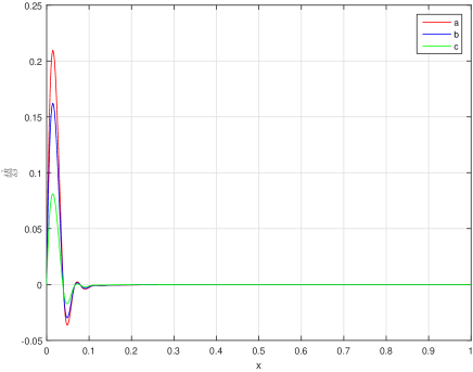
Figure 2: Case $1$: Perturbation through $K,~{}q$ and $h$. $\frac{\delta\hat{\tilde{R}}}{\delta\beta}$ as a function of $x$ for $n=1,~{}h=1.5,~{}\Gamma=1.6,~{}\alpha=0.85$, curve $a$: Q=0.2 $M_{\odot}$, curve $b$: Q=0.4 $M_{\odot}$, curve $c$: Q=0.64 $M_{\odot}$

.

Figure 3: Case $1$: Perturbation through $K,~{}q$ and $h$. $\frac{\delta\hat{\tilde{R}}}{\delta\beta}$ as a function of $x$ for $n=1,~{}h=1.5,~{}\Gamma=1.6,~{}\alpha=0.87$, curve $a$: Q=0.2 $M_{\odot}$, curve $b$: Q=0.4 $M_{\odot}$, curve $c$: Q=0.64 $M_{\odot}$

.

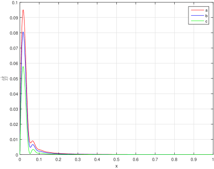
Figure 4: Case $1$: Perturbation through $K,~{}q$ and $h$. $\frac{\delta\hat{\tilde{R}}}{\delta\beta}$ as a function of $x$ for $n=1,~{}h=1.5,~{}\Gamma=1.6,~{}\alpha=0.9$, curve $a$: Q=0.2 $M_{\odot}$, curve $b$: Q=0.4 $M_{\odot}$, curve $c$: Q=0.64 $M_{\odot}$

.

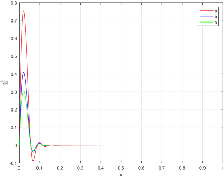
Figure 5: Case $1$: Perturbation through $n,~{}q$ and $h$. $\frac{\delta\hat{\tilde{R}}}{\delta n}$ as a function of $x$ for $n=1,~{}h=1,~{}\Gamma=1.2,~{}\alpha=0.87$, curve $a$: Q=0.2 $M_{\odot}$, curve $b$: Q=0.4 $M_{\odot}$, curve $c$: Q=0.64 $M_{\odot}$

.

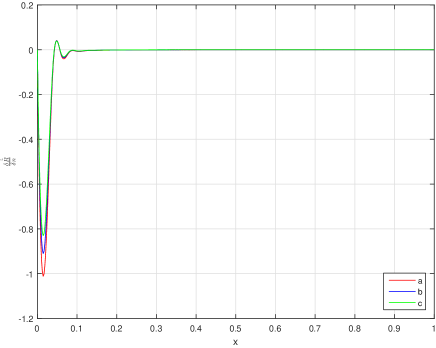
Figure 6: Case $1$: Perturbation through $n,~{}q$ and $h$. $\frac{\delta\hat{\tilde{R}}}{\delta n}$ as a function of $x$ for $n=1.5,~{}h=1.3,~{}\Gamma=0.6,~{}\alpha=0.69$, curve $a$: Q=0.2 $M_{\odot}$, curve $b$: Q=0.4 $M_{\odot}$, curve $c$: Q=0.64 $M_{\odot}$

.

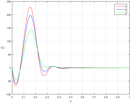
Figure 7: Case $2$: Perturbation through $K,~{}q$ and $h$. $\frac{\delta\hat{\tilde{R}}}{\delta\beta}$ as a function of $x$ for $n=0.5,~{}h=0.5,~{}\Gamma=0.6,~{}\alpha=0.69$, curve $a$: Q=0.2 $M_{\odot}$, curve $b$: Q=0.4 $M_{\odot}$, curve $c$: Q=0.64 $M_{\odot}$

.

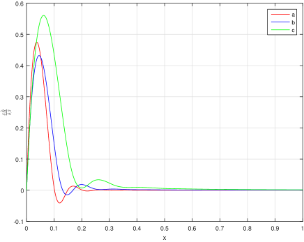
Figure 8: Case $2$: Perturbation through $K,~{}q$ and $h$. $\frac{\delta\hat{\tilde{R}}}{\delta\beta}$ as a function of $x$ for $n=0.5,~{}h=0.5,~{}\Gamma=0.6,~{}\alpha=0.90$, curve $a$: Q=0.2 $M_{\odot}$, curve $b$: Q=0.4 $M_{\odot}$, curve $c$: Q=0.64 $M_{\odot}$

.

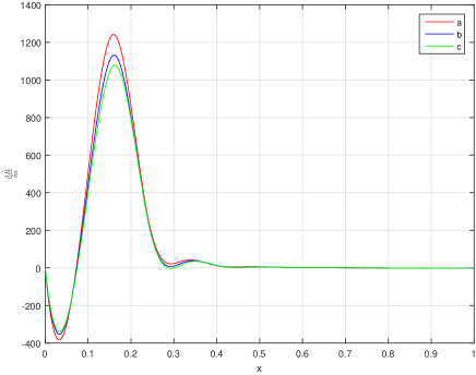
Figure 9: Case $2$: Perturbation through $n,~{}q$ and $h$. $\frac{\delta\hat{\tilde{R}}}{\delta n}$ as a function of $x$ for $n=0.5,~{}h=0.5,~{}\Gamma=0.6,~{}\alpha=0.83$, curve $a$: Q=0.2 $M_{\odot}$, curve $b$: Q=0.4 $M_{\odot}$, curve $c$: Q=0.64 $M_{\odot}$

.

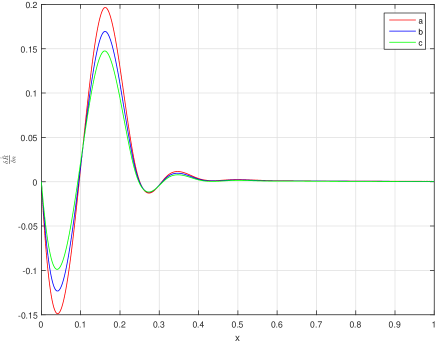
Figure 10: Case $2$: Perturbation through $n,~{}q$ and $h$. $\frac{\delta\hat{\tilde{R}}}{\delta n}$ as a function of $x$ for $n=0.5,~{}h=0.5,~{}\Gamma=0.6,~{}\alpha=0.90$, curve $a$: Q=0.2 $M_{\odot}$, curve $b$: Q=0.4 $M_{\odot}$, curve $c$: Q=0.64 $M_{\odot}$

.

Now we shall apply the formulism developed in the previous section to investigate the effects of parameters under perturbation on the stability of charged anisotropic polytropes defined by EoS $(\ref{18})$. We shall apply perturbation schemes for both types of polytropes. For this purpose, fourth-order Runge-Kutta method has been used for the integration of Eqs. $(\ref{23}),~{}(\ref{24})$ and $(\ref{61}),~{}(\ref{62})$ for any triplet of parameters $n,~{}\alpha,q$ and $n,~{}h,~{}q$ which ensure the exitance of boundary surfaces. Such values have been suggested in [19, 30]. Also, the integrals in Eqs. $(\ref{39}),~{}(\ref{54})$ and $(\ref{65})$ were integrated numerically by using trapezoidal rule. Next, we have calculated $\psi_{o}$ and $\psi$ which are used to evaluate Eqs. $(\ref{44})$ and $(\ref{58})$ for case 1 and $(\ref{63})$ and $(\ref{64})$ for case 2.

4 Discussion and conclusion

Figures 1-4 summarize the main results for polytropes of case 1, when perturbation is carried out through parameters $K,~{}q$ and $h$, whereas figs. 5 and 6 describes the behavior of polytropes when system is perturbed through parameters $n,~{}q$ and $h$. In fig.1 the cracking is appeared for $n=1,~{}h=1.5,~{}\Gamma=1.6,~{}\alpha=0.83$ and charge $Q=0.2M_{\odot}$, $Q=0.4M_{\odot}$ and $Q=0.64M_{\odot}$. We note that overturning appears in the outer regions of the model. Figures 2 and 3 describes the same behavior for $\alpha=0.85,~{}0.9$, respectively. In both cases overturning is weaker and cracking is stronger. From figs. 1-4, we finds that large value of charge $q$ leads towards weaker overturning and system become gradually stable. Figure 4 shows that for $\alpha=0.9$, system become stable. In fig. 5 strong cracking and weak overturning is noted for $n=1,~{}h=1.0,~{}\Gamma=1.2,~{}\alpha=0.87$ and for values of charge $Q=0.2M_{\odot}$, $Q=0.4M_{\odot}$ and $Q=0.64M_{\odot}$, whereas fig. 6 represent weak cracking and strong overturning for $n=1.5,~{}h=1.3,~{}\Gamma=0.6,~{}\alpha=0.69$ and for values of charge $Q=0.2M_{\odot}$, $Q=0.4M_{\odot}$, $Q=0.64M_{\odot}$, which means system remain unstable in this case.

Figures 7 and 8 sums the main results for polytropes of case 2, when perturbation is carried out through parameters $K,~{}q$ and $h$, while figs. 9 and 10 shows cracking when system is perturbed through parameters $n,~{}q$ and $h$. Figures 7 ($\alpha=0.69$) and 8 ($\alpha=0.90$) describe weak overturning near the center and strong cracking in the outer regions for $n=0.5,~{}h=0.5,~{}\Gamma=0.6$, $Q=0.2M_{\odot}$, $Q=0.4M_{\odot}$ and $Q=0.64M_{\odot}$ shown by curves a, b and c respectively. It is noted that system become stable (see fig.8 curve c) when charge increased from $Q=0.2M_{\odot}$ to $Q=0.64M_{\odot}$. Figures 9 and 10 describe a similar behavior when perturbation is carried out through $n,~{}q$ and $h$ corresponding to some fixed values.

Now, we provide a comparison between results presented in this work with those presented in [34]. The graphical analysis shows that the results obtained in this work by perturbing charge parameter differ with the one presented in [34]. If we compare the results of case 1, it is found that when perturbation is carried out by $K,~{}h$ and $q$ instead of $K,~{}h$, we note deep and strong cracking for small values of anisotropy factor $h$ and large values of alpha $\alpha$ in the presence of charge (see Figures 1-3). Further, our results (see fig.4) depicts stable configurations for increasing value of $\alpha$ in the presence of charge. Also, in case 1, it is found that both cracking and overturning appears when investigation is carried through perturbing $n,~{}q,~{}h$ instead of $n,~{}h$ shown in figs. 5 and 6, whereas the results presented in [34] shows stable configurations. A similar results have been obtained for case 2, when perturbation is carried through $K,~{}q,~{}h$. It shows that perturbing the charge parameter has a significant role on the cracking (or overturning) of polytropes.

We have developed the general procedure to investigate overturning and/or cracking of anisotropic polytropes through perturbation on anisotropy, energy density and charge. For both cases, our results have same behavior. As value of $\alpha$ increases gradually, in general the system shows strong and deep cracking and weak overturning for both cases. On the other hand, when charge increased sufficiently both configurations show stable behavior under similar conditions. It should be noted that occurrence of cracking has immediate effect on stellar structure, gravitational collapse and evolution of compact objects but the time scale chosen is much smaller then the hydrostatic time scale [33]. Moreover, the discussion of cracking and/or overturning is the study of snapshot of system just after when it leaves the equilibrium state. Also with this study one may predict about the system stability by analyzing the amplitude of cracking (or overturning) which may lead towards gravitational collapse or expansion of compact objects. The existence of charge plays an important role in the study of polytropes. As the amount of charge increase to sufficient extent, it significantly affect the existence of cracking (or overturning) phenomenon. In the concluding remarks, we can say that in some regions the existence of charge may shifts the system from unstable to stable regions even after perturbation. It is worthwhile to mentioned here that all our results reduced to [33] for anisotropic spherical polytropes in the absence of charge.

References

• [1] Chandrasekhar, S.: An introduction to the Study of Stellar Structure, University of Chicago, Chicago, (1939)
• [2] Tooper, R. F.: Astrophys. J. 140, 434 (1964)
• [3] Tooper, R. F.: Astrophys. J. 142, 1541 (1965)
• [4] Kovetz, A.: Astrophys. J. 154, 999 (1968)
• [5] Abramowicz, M. A.: Acta Astronomica 33, 313 (1983)
• [6] Bekenstein, J. D.: Phys. Rev. D 4, 2185 (1960)
• [7] Bonnor, W. B.: Zeit. Phys. 160, 59 (1960)
• [8] Bonnor, W. B.: Mon. Not. R. Astron. Soc. 129, 443 (1964)
• [9] Bondi, H.: Proc. R. Soc. Lond. A 281, 39 (1964)
• [10] Koppar, S. S., Patel, L. K., Singh, T.: Acta Phys. Hung. 69, 53 (1991)
• [11] Ray, S., Malheiro, M., Lemos, J.P.S., Zanchin, V.T.: Braz. J. Phys. 34, 310 (2004)
• [12] Herrera, L., Di Prisco, A., Ibanez, J.: Phys. Rev. D 84, 107501 (2011)
• [13] Takisa, P. M., Maharaj, S. D.: Astrophys. Space Sci. 45, 1951 (2013)
• [14] Cosenza, M., Herrera, L., Esculpi, M., Witten. L.: J. Math. Phys. 22, 118 (1981)
• [15] Herrera, L., Santos, N. O.: Phys. Rep. 286, 53 (1997)
• [16] Herrera, L., Barreto, W.: Gen. Rel. Grav. 36, 127 (2004)
• [17] Herrera, L., Di Prisco, A., Martin, J., Ospino, J., Santos, N. O., Troconis, O.: Phys. Rev. D 69, 084026 (2004)
• [18] Herrera, L., Barreto, W.: Phys. Rev. D 87, 087303 (2013)
• [19] Herrera, L., Barreto, W.: Phys. Rev. D 88, 084022 (2013)
• [20] Herrera, L., Di Prisco, A., Barreto, W., Ospino, J.: Gen. Rel. Grav. 46, 1827 (2014)
• [21] Bondi, H.: Proc. Roy. Soc. Lond. A 282, 303 (1964)
• [22] Herrera, L.: Phys. Lett. A 165, 206 (1992)
• [23] Gonzalez, G.A., Navarro, A., Nunez, L.A.: arXiv: 1410.7733.
• [24] Gonzalez, G.A., Navarro, A., Nunez, L.A.: J. Phys. Conf. Ser. 600, (2015)012014.
• [25] Azam, M., Mardan, S. A., Rehman, M. A.: Astrophys. Space Sci. 358, 6 (2015)
• [26] Azam, M., Mardan, S. A., Rehman, M. A.: Astrophys. Space Sci. 359, 14 (2015)
• [27] Azam, M., Mardan, S. A., Rehman, M. A.: Adv. High Energy Phys. 2015, 865086 (2015)
• [28] Azam, M., Mardan, S. A., Rehman, M. A.: Commun. Theor. Phys. 65, 575 (2016)
• [29] Azam, M., Mardan, S. A., Rehman, M. A.: Chin. Phys. Lett. 33, 070401 (2016)
• [30] Sharif, M., Sadiq, S.: Can. J. Phys. 93, 1420 (2015)
• [31] Azam, M., Mardan, S.A., Noureen, I. Rehman, M. A.: Eur. Phys. J. C 76, 315 (2016)
• [32] Azam, M., Mardan, S.A., Noureen, I. Rehman, M. A.: Eur. Phys. J. C 76, 510 (2016)
• [33] Herrera, L., Fuenmayor, E., A., Leon, P.,: Phys. Rev. D 93, 024247 (2016)
• [34] Sharif, M., Sadiq, S.: Eur. Phys. J. C 76, 568 (2016)
• [35] Darmois, G.: Memorial des Sciences Mathematiques, Fasc. 25 (Gautheir-Villars, 1927)
• [36] Israel, W.: Nuovo Cimento B 44S10 1 (1966);ibid. Erratum B48, 463 (1967)
• [37] Misner, C. W., Sharp, D. H.: Phys. Rev. 136, B571 (1964)