On the dearth of ultra-faint extremely metal poor galaxies

Abstract

Local extremely metal-poor (XMP) galaxies are of particular astrophysical interest since they allow us to look into physical processes characteristic of the early Universe, from the assembly of galaxy disks to the formation of stars in conditions of low metallicity. Given the luminosity-metallicity relationship, all galaxies fainter than $M_{r}\simeq-13$ are expected to be XMPs. Therefore, XMPs should be common in galaxy surveys. However, they are not, because several observational biases hamper their detection. This work compares the number of faint XMPs in the SDSS-DR7 spectroscopic survey with the expected number, given the known biases and the observed galaxy luminosity function. The faint end of the luminosity function is poorly constrained observationally, but it determines the expected number of XMPs. Surprisingly, the number of observed faint XMPs ($\sim 10$) is over-predicted by our calculation, unless the upturn in the faint end of the luminosity function is not present in the model. The lack of an upturn can be naturally understood if most XMPs are central galaxies in their low-mass dark matter halos, which are highly depleted in baryons due to interaction with the cosmic ultraviolet background and to other physical processes. Our result also suggests that the upturn towards low luminosity of the observed galaxy luminosity function is due to satellite galaxies.

1. Motivation

Galaxies having a gas-phase metallicity smaller than a tenth of the solar metallicity are often known as extremely metal-poor (XMP; e.g. Kunth & Östlin 2000). They are of astrophysical interest for a number of reasons, among which include determining the primordial He abundance produced during the Big Bang (Peimbert et al. 2010; Cyburt et al. 2016), studying star formation in conditions of low metallicity (Shi et al. 2014; Rubio et al. 2015; Elmegreen & Hunter 2015; Filho et al. 2016), understanding the formation of dust in the early Universe (Fisher et al. 2014), analyzing primitive interstellar media (Izotov & Thuan 2007), constraining the properties of the first stars (Thuan & Izotov 2005; Kehrig et al. 2015), following the assembly of primitive disks (Elmegreen et al. 2012, 2013; Sánchez Almeida et al. 2015; Ceverino et al. 2016), and studying the intergalactic gas (Sánchez Almeida et al. 2014a, b).

Unfortunately, the number of known XMPs remains small. The review paper by Kunth & Östlin (2000) contained only 31 XMPs, Kniazev et al. (2003) added 8 new targets from the early data release of the Sloan Digital Sky Survey (SDSS), the exploration in SDSS-DR6 by Guseva et al. (2009) yielded 44 sources, and the systematic bibliographic search for all XMPs in literature and the SDSS-DR7 carried out by Morales-Luis et al. (2011) rendered 140 sources. Morales-Luis et al. included targets found by Kniazev et al. (2004), Izotov et al. (2004), Izotov et al. (2006), and Izotov & Thuan (2007). Although new local metal-poor objects have been discovered since 2011 (e.g., Izotov et al. 2012; Skillman et al. 2013; James et al. 2015; Guseva et al. 2015; Sánchez Almeida et al. 2016; Hirschauer et al. 2016), XMPs remain uncommon.

The scarcity of known XMPs is in sharp contrast with the expectation that most galaxies are actually XMPs. The problem has been put forward by several authors (Skillman et al. 2013; McQuinn et al. 2013; James et al. 2015; Sánchez Almeida et al. 2016), with the following argument: there is a well-known relation between absolute luminosity or stellar mass and gas-phase metallicity (e.g., Skillman et al. 1989; Sánchez Almeida et al. 2008); consequently all faint or low-mass galaxies should be XMPs. Using as the metallicity threshold,

$$12+\log({\rm O/H})\leq 7.65,$$ (1)

the metallicity versus absolute magnitude relationship by Berg et al. (2012) implies that galaxies with absolute $B$-band magnitude

$$M_{B}\geq-12.5,$$ (2)

are XMPs. Similarly, the metallicity versus stellar mass relationship in the paper by Berg et al. (2012) entails that galaxies with stellar masses

$${\rm M}_{\star}\leq 1.1\times 10^{7}\,{\rm M}_{\odot},$$ (3)

correspond to XMP galaxies. Equation (2) can be re-written for the $r-$band magnitude using the transformation from $B$ to $r$ in Jester et al. (2005) for typical colors of gas-rich galaxies ($g-r\simeq 0.4$; Blanton & Moustakas 2009), leading to

$$M_{r}\geq-13.3.$$ (4)

Since low-mass, low-luminosity galaxies outnumber, by far, high-mass, high-luminosity galaxies (e.g., Binggeli et al. 1988; Blanton & Moustakas 2009; Kelvin et al. 2014), most galaxies are expected to be XMPs. These faint XMPs, with magnitudes and/or masses below the thresholds in Eqs. (2), (3), and (4), will be designated here as quiescent XMPs, or, QXMPs. The remaining XMPs are often denoted as active XMPs. Note that, by definition, active XMPs are low-metallicity outliers of the luminosity-metallicity relationship.

Hence, why are XMPs so unusual among the observed galaxies? It is argued that most QXMPs also have low surface brightness, so low as to be below the detection threshold of the largest surveys (see, Skillman et al. 2013; James et al. 2015).

So far as we are aware, this qualitative argument has never been quantified. In other words, (1) what is the number of QXMPs to be expected in current surveys? and, (2) is this prediction consistent with the number of known QXMPs? Our Paper addresses these two questions, finding that observational biases alone cannot account for the scarcity of observed XMPs. The luminosity function of XMP galaxies must decline for objects fainter than the limits in Eqs. (2) and (3). We show that such a drop is expected from cosmological numerical simulations, provided XMPs are central, rather than, satellite galaxies. The ultraviolet (UV) background is then expected to prevent the formation of low-mass galaxies (e.g., Efstathiou 1992; Thoul & Weinberg 1996; Kravtsov et al. 2004; Wyithe & Loeb 2006; Okamoto et al. 2008). Several physical processes may suppress gas accretion and star formation in low-mass dark matter halos. The cosmological UV background heats the intergalactic gas and establishes a minimum mass for halos that can accrete gas. The gas in low-mass halos may also be photo-evaporated by the UV background after re-ionization. In addition, the ionizing radiation dissociates molecular hydrogen, which is the main coolant for low-metallicity gas, thus preventing star formation even before the gas is completely stripped from the halos by other quenching processes. Stellar feedback processes, such as supernova explosions and stellar winds, are also able to remove gas from galaxy disks, reducing the star formation efficiency in low mass halos, where the gravitational binding energy is particularly low (e.g., White & Frenk 1991; Dalla Vecchia & Schaye 2008; Governato et al. 2010; Silk & Mamon 2012; Vogelsberger et al. 2014; Schaye et al. 2015). Thus, when the galaxy has a stellar mass smaller than several $10^{8}\,M_{\odot}$, most of the gas that could be used to form stars returns unused to the inter-galactic medium (e.g., Davé et al. 2012; Shen et al. 2012; Sánchez Almeida et al. 2014a; Christensen et al. 2016).

The paper is organized as follows: Section 2 describes the number of QXMPs observed in the spectroscopic sample of the SDSS-DR7, which is chosen because this survey provides most of the known XMPs. Section 3 is devoted to estimating the expected number of QXMPs from the galaxy luminosity function, by firstly extrapolating the observed luminosity function to faint objects, and then including the effect of the baryon fraction changing with the dark matter halo mass (Sect. 3.3). The results are discussed in Section 4, including an analysis of the factors that limit the number of observed QXMPs, and how they can be overcome in future searches (Sect. 4.2). The number of observed QXMPs to be expected in other existing and forthcoming surveys is determined in Section 4.3. The results are collected and summarized in Section 5. Throughout the paper, the Hubble constant $H_{0}$ is taken to be 70 km s^-1 Mpc^-1.

2. Number of observed QXMPs in the SDSS-DR7

The search for XMPs during the last decade has been very much focused on the spectroscopic sample of the SDSS-DR7 (Abazajian et al. 2009). The purpose of this section is to evaluate how many QXMPs have been found as part of these SDSS-DR7-based searches. A comprehensive list is needed to compare the number of observed and expected QXMPs.

We have built the list by searching all recent papers that may have XMPs from the SDSS-DR7. The galaxies in this paper were filtered so as to keep only those from the SDSS-DR7 with metallicity and luminosity below the thresholds in Eqs. (1) and (4), respectively. The samples that were analyzed are:

1. The Morales-Luis et al. (2011, ML+11) XMP sample, which contains a compilation of all low metallicity ($12+\log[{\rm O/H}]\lesssim 7.65$) sources from the literature until the date of publication, plus several new targets from the SDSS-DR7 spectroscopic sample. It uses photometry from the SDSS.

2. The Sánchez Almeida et al. (2016, SA+16) XMP sample from the SDSS-DR7, with metallicity from SDSS spectra, and photometry also from the SDSS.

3. The Karachentsev et al. (2013, Kara+13) sample, which is the latest version of the nearby galaxy reference catalog. Only sources with $M_{B}\geq-12.5$ mag are considered here, where both the metallicity and photometry are compiled from literature.

4. The Berg et al. (2012, Berg+12) sample, a subsample of low-luminosity galaxies within 11 Mpc, with metallicities and photometry from Multiple Mirror Telescope (MMT) observations.

5. The Izotov et al. (2012, Izo+12) sample, a study of metal-poor emission-line SDSS-selected galaxies, with metallicities from Apache Point Observatory (APO) 3.5 m and/or MMT, and photometry from the SDSS.

6. The James et al. (2015, James+15) sample, a set of SDSS-selected blue diffuse dwarf galaxies, with metallicities from MMT observations and photometry from the SDSS.

From these six samples, we selected galaxies fulfilling the following criteria: (a) appear in the SDSS-DR7 spectroscopic catalog, (b) their $B$-band absolute magnitudes are larger than -12.5, and (c) have metallicities $12+\log({\rm O/H})\leq 7.65$. For the resulting sources, we checked whether the photometry was reliable, particularly in those cases where only SDSS photometry is available. For the SDSS photometry, we first visually inspected the SDSS images of the sources and registered the source size. The visual sizes were then compared with the SDSS Petrosian g-band radius at 90% of the light, obtained at the position of the SDSS spectroscopic target. If the sizes were well-matched, the SDSS photometry was deemed reliable, and the source was retained as a QXMP. If the sizes were not well-matched, we then looked into literature for a value for the photometry. Most of them happen to have alternative photometry, which allowed us to exclude 90 %  of them as QXMPs. Only three objects had no alternative photometry, and they were discarded by the argument that their chance of being an QXMP is the same as those with photometry. This chance is only 10 %, which amounts to 0.3 sources.

Figures 1a and 1b summarize the selection procedure and its outcome. They show oxygen abundance versus absolute $B$ magnitude for the galaxies in the previous references. In order to avoid overcrowding, the samples are split into two plots, and only XMPs with reliable magnitudes are shown for $M_{B}>-12.5$. Figure 1a contains the compilation ML+11, plus the XMPs from the SDSS-DR7 recently identified in SA+16. There are only five targets with $M_{B}>-12.5$ that seem to be bona-fide QXMPs in the SDSS-DR7 spectroscopic database. Those are encircled with black outlines in Fig. 1a. One of these appears in the two samples with slightly different magnitude and metallicity; the two corresponding points are encircled together.

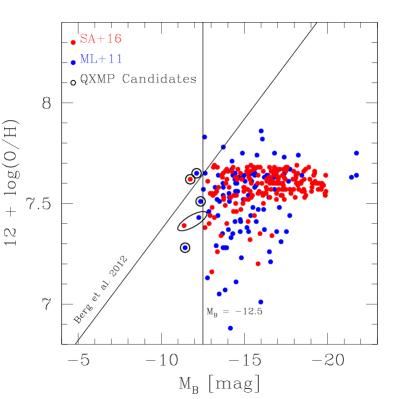
Figure 1.— Oxygen abundance vs absolute $B$ magnitude for galaxies found in recent searches containing XMPs. We are interested in those objects that are QXMPs (i.e., to the left of the vertical black solid lines, $M_{B}=-12.5$) and which simultaneously appear in the SDSS-DR7 spectroscopic sample. The luminosity-metallicity relationship by Berg et al. (2012), used to define QXMPs, is included. (a) Compilation by Morales-Luis et al. (2011, blue symbols) of all XMPs in the literature up to the date of publication, and high-electron temperature XMPs from the SDSS-DR7 by Sánchez Almeida et al. (2016, red symbols). Only the five encircled objects are bona-fide QXMPs in the SDSS-DR7 spectroscopic sample. One of these appears in the two samples with slightly different magnitude and metallicity; the two corresponding points are encircled together. (b) Objects from Karachentsev et al. (2013, green symbols), Izotov et al. (2012, brown symbols), James et al. (2015, purple symbols), and Berg et al. (2012, magenta symbols). The prototype QXMP Leo P (Skillman et al. 2013) and the recently discovered AGC 198691 (Hirschauer et al. 2016) are also included in the figure for reference, even though they are not part of the SDSS-DR7 spectroscopic sample. Four new QXMPs have been identified, and are marked with a solid outline. One of the four (J1056+36) has three HII regions having slightly different abundances. The objects with the dashed outlines are QXMPs already included in (a) –two of these have two different abundance estimates so that the dashed outline is elongated.

Figure 1b contains the low-luminosity objects with measured metallicity from the four remaining samples: Kara+13 (green symbols), Izo+12 (brown symbols), James+15 (purple symbols), and Berg+12 (magenta symbols). The galaxies in Berg+12 are those used to derive the luminosity-metallicity relationship leading to the QXMP magnitude limit in Eq. (2); the relationship is shown as a slanted black line in Figs. 1a and 1b. The prototype QXMP Leo P (Skillman et al. 2013) and the recently discovered AGC 198691 (Hirschauer et al. 2016) are also included in the figure for reference, even though they do not belong to the SDSS-DR7 spectroscopic sample. After a screening similar to the one carried out with the objects in Fig. 1a, we are left with only four new targets outlined with solid lines in Fig. 1b. The samples represented in Fig. 1b contain 4 additional QXMPs, which are outlined with dashed lines in the figure. They are already in the samples by ML+11 or SA+16, and so, they do not contribute to the total number of QXMPs.

At the end of our selection process, we are left with nine QXMPs, i.e.,

$$N^{\rm obs}_{\rm QXMP}=9\pm 3,$$ (5)

where the error considers only the Poissonian statistical error associated with the process of counting (e.g., Martin 1971). It is important to realize that Eq. (5) probably represents an upper limit. Since QXMPs are so uncommon, the chances of having false positives (non-QXMP galaxies misidentified as QXMP) are expected to be much greater than the chances of having false negatives (QXMPs excluded by mistake). The coordinates and main properties of the nine QXMPs are listed in Table 1, while their SDSS images are shown in Fig. 2. Many of them are contained transversally in more than one of the analyzed samples.

Table 1Bona-fide QXMPs in the SDSS-DR7 spectroscopic survey.

Name a	$12+\log({\rm O/H})$	$M_{B}$	$M_{r}$	$SB_{r}$	D b	Reference	Also in
				[mag arcsec-2]	[Mpc]	c	c
J084338.0+402547.1	$7.57\pm 0.06$	-12.3	-12.8	22.1	10.2	Izo+12	–
J091159.4+313534.4	$7.51\pm 0.14$	-12.4	-12.7	21.9	11.6	ML+11	–
J095905.7+462650.5	$7.50\pm 0.05$	-12.3	-11.9	24.0	8.0	Izo+12	–
J105640.3+360827.9	$7.26\pm 0.09$	-12.1	–	–	9.2	Kara+13 ($M_{B}$)	Izo+12 ($12+\log[{\rm O/H}])$
J115754.2+563816.7	$7.62\pm 0.11$	-11.7	-12.1	22.3	5.8	SA+16	Kara+13, James+15
J121546.6+522313.8	$7.39\pm 0.15$	-11.4	-11.6	22.5	2.1	SA+16	ML+11, Berg+12
J123109.1+420533.9	$7.62\pm 0.04$	-12.2	-12.1	23.8	8.2	Izo+12	Kara+13
J123839.1+324555.9	$7.28\pm 0.07$	-11.4	–	–	3.1	ML+11	Kara+13, Berg+12
J125840.1+141308.1	$7.65\pm 0.06$	-12.1	–	–	2.2	ML+11	Kara+13, Berg+12

a The name includes the coordinates RA and DEC.

b Distance adopted in the respective reference to determine absolute magnitudes.

c Morales-Luis et al. (2011, ML+11), Izotov et al. (2012, Izo+12), Berg et al. (2012, Berg+12),

Karachentsev et al. (2013, Kara+13), James et al. (2015, James+15), Sánchez Almeida et al. (2016, SA+16).

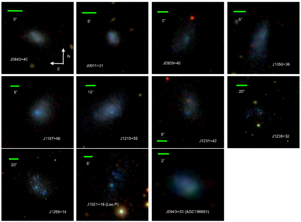
Figure 2.— Images of the nine QXMPs in the SDSS-DR7 spectroscopic survey, with the names given in the insets. Their properties are listed in Table 1. Although the prototype QXMP Leo P is not in the SDSS-DR7 spectroscopic survey, it is included for reference. The same happens with AGC 198691. The orientation of all images is given by the arrows in the first image, with the angular size shown in the individual images by the green scale.

As we argue in Sect. 1, QXMPs are expected to have low surface brightness (SB). Figure 3 shows the SB versus absolute magnitude in the $r$-band for the QXMPs with reliable SDSS photometry. All surface brightnesses referred to in the paper are half-light surface brightnesses. Despite their low SB (22 – 24 mag arcsec^-1; see Fig. 3 and Table 1), they tend to be brighter than expected from extrapolating the relationship between magnitude and SB found for brighter galaxies (the black solid line in Fig. 3, from Blanton et al. 2005). Only two of the targets appear to follow the relationship (J0959+46 and J1231+42; compare their images with Leo P in Fig. 2).

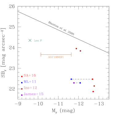
Figure 3.— $SB_{r}$ versus $M_{r}$ for the QXMP with spectra in the SDSS-DR7 and reliable SDSS photometry. Leo P and AGC 198691 are also included for reference. Note that they are high-SB outliers of the $SB_{r}$ versus $M_{r}$ relationship found for brighter objects, and extrapolated to fainter galaxies in this plot (the black solid line). The pairs of points joined by dashed lines correspond to the same object reported in two different samples.

The origin of this unexpectedly large SB can be pinned down to the bias of the observation toward high-SB objects, and the intrinsic scatter in the relationship between SB and magnitude. Given an absolute magnitude, observations preferentially pick up the objects of largest SB. This scatter is important for estimating the expected number of QXMPs, and so it is discussed and treated in Sect. 3.2 and the Appendix.

3. Number of faint XMPs to be expected in the SDSS-DR7

3.1. Calculation of the expected number of QXMPs

The galaxy luminosity function (LF), $\Phi(M)$, is defined as the number of galaxies with absolute magnitude $M$, per unit volume and unit magnitude. Figure 4a shows the LF in the $r$-band determined by Blanton et al. (2005) from the SDSS-DR2 data. The number of galaxies in a survey fainter than a given limiting magnitude, $M_{lim}$, is

$$N(M>M_{lim})=\int^{M_{1}}_{M_{lim}}S(M)\,\Phi(M)\,dM,$$ (6)

with $S(M)$ the selection function that provides the effective volume that is sampled by the survey. Equation (6) assumes $S$ to depend only on the absolute magnitude of the galaxy, which is reasonable in our case, and simplifies the treatment. This assumption will be relaxed later on. Equation (6) also assumes the existence of a limit for the magnitude of the faintest galaxy, $M_{1}$.

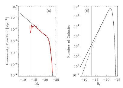
Figure 4.— (a) Galaxy LF in the $r$-band from Blanton et al. (2005). The red line shows the actual data, whereas the black solid line represents a double Schechter function fit, which we use to describe the number of QXMPs with magnitudes to the left of the vertical black solid line. (b) Number of galaxies per unit magnitude to be expected from the SDSS-DR7 spectroscopic survey. The black solid line shows the effect of the Malmquist bias (apparent magnitude limit cutoff), whereas the black dashed line also includes the incompleteness for low-SB objects.

In the case of a volume-limited sample, $S$ is just the volume of the sample, and so independent of the absolute magnitude. In the case of an apparent magnitude-limited survey, where all galaxies brighter than the apparent magnitude, $m_{lim}$, are included, $S(M)$ is the volume where galaxies of magnitude $M$ have apparent magnitude $m_{lim}$ or brighter, i.e.,

$$S(M)=V(M)={{d^{3}}\over{3}}\Omega,$$ (7)

with $\Omega$ the solid angle covered by the survey, and $d$ the maximum distance at which a galaxy of magnitude $M$ can be observed, i.e.,

$$\log(d)={{1}\over{5}}(m_{lim}-M)-5,$$ (8)

with $d$ in Mpc. The SDSS spectroscopic survey was designed to be apparent magnitude-limited, with a limit in the $r$-band given by

$$m_{lim}=17.77.$$ (9)

In practice, all surveys have a limit in surface brightness. Blanton et al. (2005) work it out for the SDSS, showing that the completeness of the spectroscopic survey decreases drastically for an average surface brightness, $SB_{r}$, fainter than 23 mag arcsec^-2, reaching only 10 % completeness at 24 mag arcsec^-2. This bias against low-SB objects is particularly severe for QXMPs. Galaxies fainter than the limit in Eq. (2) may, in principle, have any surface brightness. However, faint galaxies tend to have a low SB as well (e.g., Kormendy 1985; Skillman 1999). Blanton et al. (2005) give the following relationship between surface brightness and absolute magnitude in the $r$-band,

$$SB_{r}=23.8+0.45\,(M_{r}+13.3).$$ (10)

This relationship is in close agreement with others found in literature (e.g., Kormendy 1985; Geller et al. 2012), and appears to be valid down to very low magnitudes (even for $M_{B}>-8$; e.g., Karachentsev et al. 2013). Equation (10) implies that galaxies fainter than the QXMP limit (Eq. [4]) are fainter than 23.8 mag arcsec^-2, and so, potentially subject to severe incompleteness in the SDSS. Completeness is quantified using the completeness function, which gives the fraction of galaxies with a given SB that are detected in the survey, $C^{\prime}(SB)$. Combining the SDSS completeness function by Blanton et al. (2005, Fig. 3) with Eq. (10), one finds the completeness function, $C(M)$, in Fig. 5 (the symbols joined by a solid line). Including completeness,

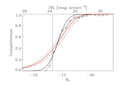
Figure 5.— Completeness function for the SDSS due to the low SB of the targets. The symbols joined by a solid line combine the total completeness estimated by Blanton et al. (2005) with the relation between $SB_{r}$ and $M_{r}$ in Eq. (10). This completeness function is approximated in the analysis by the erf function shown as a thick solid line. The red solid line is the effective completeness function resulting from the scatter in the $SB_{r}$ vs $M_{r}$ relationship. The black dotted and dashed lines are the red solid line shifted by plus and minus half a magnitude, respectively, and encompass the statistical error of the completeness function. The vertical black line, $M_{r}=-13.3$, marks the QXMP limit. The axis on top gives the $SB_{r}$ in mag arcsec^-2, corresponding to the absolute magnitudes in the bottom axis.

the selection function turns out to be

$$S(M)=V(M)\,C(M),$$ (11)

which remains a function of the absolute magnitude only. As we show in the Appendix, Eq. (11) remains formally valid when the scatter of the relationship between $SB$ and $M$ is taken into account. This scatter is bound to be important in the analysis, since most observed QXMPs are high-SB outliers of the $SB_{r}$ versus $M_{r}$ relationship (Fig. 3). In this case, the completeness, $C(M)$, in Eq. (11) must be replaced with an effective completeness,

$$S(M)=V(M)\,C_{eff}(M),$$ (12)

where

$$C_{eff}(M)=\int_{\forall\,SB}P(SB|M)\,C^{\prime}(SB)\,dSB.$$ (13)

$P(SB|M)$ stands for the conditional probability function of having a surface brightness $SB$ when the magnitude of the galaxy is $M$. $C^{\prime}(SB)$ represents the completeness function in terms of $SB$. $P(SB|M)$ is also provided by Blanton et al. (2005) (see Appendix A), and the resulting $C_{eff}(M)$ is represented in Fig. 5 as the red solid line. In order to evaluate the integral in Eq. (13), we use an erf function fit to the actual discrete completeness measured by Blanton et al. (2005) (i.e., we use the smooth thick solid line in Fig. 5, meant to reproduce the symbols). As can appreciated in Fig. 5, the scatter increases the effective completeness of the survey at low SB, and this occurs because many targets happen to have a SB larger than that assigned by Eq. (10), and those are the ones that are preferentially selected.

The integrand of Eq. (6) gives the number of galaxies of a given magnitude to be expected in a survey. Figure 4b shows this integrand for the SDSS-DR7 spectroscopic survey, which implies employing the $m_{limit}$ in Eq. (9), and $\Omega=2.45\,$srad (Abazajian et al. 2009). We use the LF for extremely low-luminosity galaxies determined by Blanton et al. (2005). The actual LF is shown as the red solid line in Fig. 4a, although we use for the calculations the double Schechter function fitted to the observations by Blanton et al. (2005), i.e.,

$$\Phi(M)=(0.4\,\ln 10\,h^{3}\,{\rm Mpc}^{-3})\,{\Large\exp}\big{[}-10^{-0.4\,(M-M_{\star})}\big{]}\,\times$$ (14)

$$\big{[}\phi_{\star,1}\,10^{-0.4\,(M-M_{\star})*(1+\alpha_{1})}+\phi_{\star,2}\,10^{-0.4\,(M-M_{\star})*(1+\alpha_{2})}\big{]}$$

with $\phi_{\star,1}=0.0134$, $\phi_{\star,2}=0.0086$, $\alpha_{1}=0.33$, $\alpha_{2}=-1.40$, $M_{\star}=-19.99-5\,\log h$, and $h$ is the Hubble constant normalized to 100 km s^-1 Mpc^-1. This double Schechter function is shown as the black solid line in Fig. 4a. Thus, our estimates are based on the extrapolation to low luminosity of the observed LF, which yields a function that continues growing towards the region occupied by the QXMPs (to the left of the vertical black line in Fig. 4a). Assuming the Malmquist bias alone, i.e., using Eq. (7) for the selection function, the number of expected QXMPs, $N_{\rm QXMP}$, is 149 (see Table 2). This figure results from integrating the solid line in Fig. 4b up to the QXMP threshold. When the full selection function is considered (Eq. [12]), the total number of expected QXMP galaxies turns out to be

$$N_{\rm QXMP}\simeq 42.$$ (15)

We integrate from $M_{r}=-13.3$ to $-8$. The upper limit is taken from Karachentsev et al. (2013, Fig. 10) as the faintest magnitude of the late-type galaxies in the local Universe. This upper limit, however, does not affect $N_{\rm QXMP}$ since the selection function is very small at low luminosities. Even though the number in Eq. (15) represents a minuscule fraction of the galaxies to be expected in the full survey (1.1$\times 10^{6}$; Table 2), the actual number exceeds the $9\pm 3$ QXMP galaxies that are observed (Sect. 2). The predicted $N_{\rm QXMP}$ depends on the completeness function, and it falls off towards low SB, which is uncertain. We work out the error budget in Sect. 3.2, yielding a number of expected QXMPs between 12 and 73, with the high value range strongly favored. Thus, the discrepancy between observations and predictions remains even when uncertainties are taken into account.

Our detailed description of differences between the number of observed and predicted QXMPs should not override the fact that these two numbers are always very small. QXMPs are, at most, a few tens in a survey such as the SDSS-DR7, which contains almost one million galaxies with spectra. QXMPs outnumber any other type of galaxy, but only a tiny fraction of these is detected: in the prediction described above, 87 % of the galaxies are QXMPs, but they constitute only 0.004 % of the detected galaxies (Table 2). The actual percentages depend on the specific assumptions (see Table 2), but the vast disproportion between the true number of QXMPs and their paucity in surveys always holds true.

Table 2Number of galaxies to be expected in a SDSS-DR7-like survey.

Description	Number or Percentage	Comment
Total number a, LF with $C\not=1$	$1.1\times 10^{6}$	dashed line in Fig. 4b
QXMP, $C=1$	149	solid line in Fig. 4b
QXMP, $C\not=1$	42	dashed line in Fig. 4b
	12 — 73	uncertainties in Sect. 3.2
% QXMP in the survey	0.004
% QXMP in a volume$\,{}^{b}$	87
Total number a, varying $f_{b}$, $C\not=1$	$1.1\times 10^{6}$	red dashed line in Fig. 6b
QXMP, $C=1$	20	red solid line in Fig. 6b
QXMP, $C\not=1$	6	red dashed line in Fig. 6b
	3 — 12	uncertainties like in Sect. 3.2
% QXMP in the survey	0.0005
% QXMP in a volume$\,{}^{b}$	45
Total number a, exponential $f_{b}$, $C\not=1$	$1.1\times 10^{6}$	green dashed line in Fig. 6b
QXMP, $C=1$	24	green solid line in Fig. 6b
QXMP, $C\not=1$	7	green dashed line in Fig. 6b
	4 — 15	uncertainties like in Sect. 3.2
% QXMP in the survey	0.0006
% QXMP in a volume$\,{}^{b}$	42
Total number a, LF for centrals$\,{}^{c}$	$0.8\times 10^{6}$	solid line in Fig. 8b
QXMP, $C=1$	15	solid line in Fig. 8b
QXMP, $C\not=1$	4	dashed line in Fig. 8b
	3 — 9	uncertainties like in Sect. 3.2
% QXMP in the survey	0.0005
% QXMP in a volume$\,{}^{b}$	52

a The real SDSS-DR7 spectroscopic survey has $0.93\times 10^{6}$ galaxies (Abazajian et al. 2009).

b In an unbiased, purely volume-limited survey.

c From Yang et al. (2009).

3.2. Error budget for the expected number of QXMPs

The number of QXMPs depends on several assumptions, as explained in the previous section. Those assumptions are modified here to determine their impact on the estimated number of QXMPs.

1. Neglecting the scatter in the $SB_{r}$ versus $M_{r}$ relationship. The scatter increases the effective completeness quite substantially. If the scatter is neglected then one is left with the completeness function, $C$; either the actual completeness determined by Blanton et al. (2005, the symbols in Fig. 5) or the erf function fit to this completeness (the smooth solid black line in Fig. 5). If the actual completeness is used, then $N_{\rm QXMP}\simeq 12$. If the erf fit is used, then $N_{\rm QXMP}\simeq 19$. These estimates are closer to (but still larger than) the number of observed QXMPs (Eq. [5]). However, they must be regarded as lower limits to the predicted $N_{\rm QXMP}$. The scatter in the $SB_{r}$ versus $M_{r}$ relationship is a key ingredient of the detection process, as proven by the fact that the observed QXMPs are high-SB outliers of the extrapolated $SB_{r}$ versus $M_{r}$ relation (Fig. 5). Consequently, the scatter must be included, and $N_{\rm QXMP}\geq 12$.

2. The completeness function. We have used the erf fit to the completeness function by Blanton et al. (2005) to evaluate the effective completeness leading to the limit in Eq. (15). If rather than the fit, the actual completeness is used (i.e., the symbols in Fig. 5), then $N_{\rm QXMP}\simeq 38$. The difference between the erf and the completeness by Blanton et al. (2005) is about $\pm 0.5$ mag, in the sense that if the erf fit is shifted by $\pm 0.5$ mag then it encompasses all the points. If the effective completeness is evaluated using the completeness shifted by $\pm 0.5$ mag, one obtains the black dashed and dotted lines in Fig. 5. They yield a $N_{\rm QXMP}$ between 36 and 50.

3. The absolute magnitude limit. The absolute magnitude limit to be an QXMP, given in Eq. (4), depends on a number of factors. The value of this limit is relevant because the majority of the QXMPs are within one magnitude of the cut-off (i.e., the number of QXMPs is dominated by objects with metallicity just below the metallicity cut-off and its corresponding absolute magnitude). If we use exactly 1/10 of the solar abundance by Asplund et al. (2009), then the limit in Eq. (1) becomes 7.69, so that the mass-metallicity relationship by Berg et al. (2012) predicts $M_{B}\geq-12.9$, and the limit in the $r$-band becomes $M_{r}\geq-13.7$. This brighter limit allows for more QXMPs, specifically, $N_{\rm QXMP}\simeq 73$. The conversion from Eq. (3) to Eq. (4) employs both the magnitude transformation by Jester et al. (2005) and a single color $g-r\simeq 0.4$ for all galaxies. If one uses the full range of colors for galaxies in the blue cloud, $0.2\leq g-r\leq 0.6$ (e.g., Blanton & Moustakas 2009), then $M_{r}$ goes from -13.0 to -13.5, which renders $N_{\rm QXMP}$ from 28 to 55. Finally, if the uncertainties in the relation derived by Berg et al. (2012) are propagated into the magnitude cutoff, then $M_{B}\geq-12.5\pm 0.3$, and so $M_{r}\geq-13.3\pm 0.3$, leading to values of $N_{\rm QXMP}$ between 28 to 64.

4. The relationship between absolute magnitude and surface brightness. The relationship between the absolute magnitude and surface brightness in Eq. (10) is given by Blanton et al. (2005). In order to test the uncertainty introduced by the use of this relationship, we also employed the law for blue objects by Geller et al. (2012), $SB_{r}=29.9+0.46\,M_{r}$, and by Kormendy (1985), $SB_{r}=30.3+0.47\,M_{r}$. The latter was digitized from Fig. 3 in Kormendy’s paper. The magnitudes were then transformed from $V$ and $B$ to $r$ (Jester et al. 2005), and the central surface brightness was converted to the half-light surface brightness assuming an exponential light profile. The use of these two alternative relationships renders a $N_{\rm QXMP}$ always around 42.

5. A combination of the previous assumptions. In the previous items, the ingredients that determine $N_{\rm QXMP}$ are analyzed independently. We have also checked the combined effect of all of them operating simultaneously. We carried out a Monte Carlo simulation where $N_{\rm QXMP}$ was estimated varying the completeness function, the magnitude limit, and the mapping between $SB_{r}$ and $M_{r}$, simultaneously. Explicitly, the center of the completeness function and the absolute magnitude limit were randomly changed following Gaussian distributions with standard deviations of 0.5 mag (item # 2) and 0.3 mag (item # 3), respectively. In addition, the three relations between $SB_{r}$ and $M_{r}$ discussed in item # 4 were assumed to be equally probable. As a result of 1000 trials, we obtain $N_{\rm QXMP}=46\pm 20$, which is similar to the range of values inferred from the individual factors separately (Table 2).

6. The adopted LF. We separate the properties of the LF into two parts: the shape and the normalization. Changes in the shape are analyzed in Sect. 3.3, and produce significant changes in the number of expected QXMPs. The normalization, however, is fairly well-constrained by the total number of galaxies in the SDSS-DR7 spectroscopic sample, which amount to $0.93\times 10^{6}$ galaxies. By scaling the LF to reproduce the actual number of sources in the DR7 (i.e., to go from 1.1 million to 0.93 million; see Table 2) one finds $N_{\rm QXMP}\simeq 35$.

3.3. Including galaxy formation quenching induced by the UV background

As we have shown above, the number of observed QXMPs (around 9; Eq. [5]) is not consistent with the number of QXMPs expected from extrapolating the observed LF to low luminosities (from 12 to 73, with the best value around 42; Table 2). Such an extrapolation of the LF implicitly neglects the quenching of galaxy formation in low-mass halos expected from numerical models of galaxy formation (see Sect. 1). These predict a rapid fall-off of the baryon fraction, $f_{b}$, in low-mass halos due to various physical processes, such as heating of the intergalactic medium by the UV background or stellar feedback (see Sect. 1). The drop in $f_{b}$ induces a drop in the gas that fuels star formation, and, hence, a drop in the number of the low-mass, low-luminosity galaxies affected by the decrease of baryons.

The effect of the baryon fraction on the LF can be modeled considering that the magnitude of a galaxy is related to the baryon fraction as follows,

$$M-M^{\odot}=-2.5\log\big{[}f_{L}\,(1-f_{g})\,f_{b}\,\mu\big{]},$$ (16)

where $M^{\odot}$, $f_{L}$, and $f_{g}$ stand for the absolute solar magnitude, the light-to-stellar mass ratio (in solar units), and the gas fraction, respectively. The symbol $\mu$ in Eq. (16) stands for the total mass, including dark matter, gas and stars. Equation (16) allows us to express $\Phi$ in terms of the LF obtained assuming the baryon fraction to be constant, $\Phi_{0}$. In this case, the mapping between $M$ and the magnitude $M_{0}$ when $f_{b}$ is a constant equal to $f_{b0}$ turns out to be

$$M-M_{0}=-2.5\log\big{[}f_{b}/f_{b0}\big{]},$$ (17)

so that the LFs for $\Phi(M)$ and $\Phi_{0}(M_{0})$ are linked by (e.g., Martin 1971),

$$\Phi(M)=\Phi_{0}(M_{0})\,{{dM_{0}}\over{dM}}.$$ (18)

The ratio between the two luminosity functions at the same magnitude, $X(M)$, quantifies the drop in LF induced by the drop in the baryon fraction, i.e.,

$$X(M)={{\Phi(M)}\over{\Phi_{0}(M)}}={{\Phi_{0}(M_{0})}\over{\Phi_{0}(M)}}\,{{dM_{0}}\over{dM}}.$$ (19)

Neglecting variations with halo mass of the mass-to-light ratio and the gas fraction, then

$${{dM_{0}}\over{dM}}={{dM_{0}/d\mu}\over{dM/d\mu}}={1\over{1+d\ln f_{b}/d\ln\mu}}.$$ (20)

The baryon fraction is usually expressed in terms of the half-fraction mass, so that at mass $\mu=\mu_{c}$ the baryon fraction, $f_{b}$, is half the cosmic baryon fraction $\langle f_{b}\rangle$. In the parametrization determined by Gnedin (2000), and then adopted by many others,

$$f_{b}=\langle f_{b}\rangle\big{[}1+(2^{a/3}-1)(\mu/\mu_{c})^{-a}\big{]}^{-3/a},$$ (21)

with $a\simeq 2$, as constrained by numerical simulations (Okamoto et al. 2008). Numerical simulations also give $\mu_{c}\simeq 9.3\times 10^{9}\,{\rm M}_{\odot}$ in the local Universe at redshift zero (Okamoto et al. 2008, Fig. 3). If the baryon fraction is given by Eq. (21), then the transformation between $\Phi_{0}$ and $\Phi$ can be computed analytically, since

$${{d\ln f_{b}}\over{d\ln\mu}}={{3(2^{a/3}-1)}\over{1+(2^{a/3}-1)(\mu_{c}/\mu)^{a}}}({{\mu_{c}}\over{\mu}})^{a}.$$ (22)

It is important to realize that, in the limit of very low luminosities, $\mu\ll\mu_{c}$, so that Eq. (22) predicts

$${{d\ln f_{b}}\over{d\ln\mu}}\simeq 3.$$ (23)

Therefore, there is a drop of the LF associated with the vanishing baryon fraction, but it is not very large,

$$\Phi(M){\Big{/}}\Phi_{0}(M_{0})\simeq 0.25\,.$$ (24)

In fact, $\Phi(M)$ flattens for very low masses because, for a given variation of $M$, $M_{0}$ changes very little, so that $\Phi_{0}(M_{0})$ in Eq. (24) is approximately constant, and $\Phi({\rm M})$ becomes independent of $M$ also. The LFs in Fig. 6a show this behavior – see the red solid line, which is computed from Eqs. (18), (17), (20), (21), and (22) with $\langle f_{b}\rangle=0.158$ (Planck Collaboration et al. 2016), $f_{b0}=\langle f_{b}\rangle$, $f_{L}=1$, and $f_{g}=0.9$.

The damping of the LF caused by the baryon fraction in Eq. (21) is never very large. In order to make the drop more pronounced, we also tried a negative exponential parametrization of the baryon fraction,

$$f_{b}=\langle f_{b}\rangle\,{\Large\exp}(-{{\mu_{c}\ln 2}\over{\mu}}),$$ (25)

which is hardly distinguishable from Eq. (21) in the representation used to compare with numerical simulations (see Fig 7a), but which produces a linear drop of the luminosity function (Fig. 7b), since

$${{d\ln f_{b}}\over{d\ln\mu}}=\mu_{c}\ln 2/\mu,$$ (26)

so that, at low luminosity, where $\mu\ll\mu_{c}$,

$$\Phi(M)/\Phi_{0}(M_{0})\simeq{\mu/(\mu_{c}\ln 2)}\longrightarrow 0.$$ (27)

The LF resulting from the exponential fall-off of the baryon fraction is shown as a green solid line in Fig. 6a.

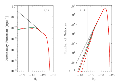
Figure 6.— (a) Galaxy LF in the $r$-band from Blanton et al. (2005) (black solid line, which is identical to the black solid line in Fig. 4a). If the effect of the varying baryon fraction is considered, the LF becomes flat at low luminosities, as shown by the colored lines. The red line corresponds to the variation computed by Okamoto et al. (2008), whereas the green line represents an exponential drop. (b) Number of galaxies per unit magnitude to be expected from the SDSS-DR7 spectroscopic survey. The color code is the same as in (a). The solid lines show the effect of the Malmquist bias (an apparent magnitude threshold), whereas the black dashed lines also include the incompleteness for low-SB objects.

Figure 7.— Comparison between the two baryon fractions used in this work. (a) Baryon fraction versus total mass for the two parameterizations: the one by Gnedin (the solid line) and the exponential drop (the black dashed line). In both cases, the half-fraction mass, $\mu_{c}$, has been set to $9.3\times 10^{9}\,{\rm M}_{\odot}$, with the universal baryon fraction given by $\langle f_{b}\rangle=0.158$ (the black dotted line). (b) Drop in the LF versus absolute magnitude produced by the two baryon fractions. The one by Gnedin saturates at 0.25 (the solid line), whereas the exponential drop continues to decrease to infinity. Magnitudes are computed from total masses using the same parameters for the two baryon fractions, namely, a stellar mass-to-light ratio of 1 solar mass per solar luminosity, and a gas-to-stellar mass fraction of $f_{g}=0.9$. The vertical black dotted line denotes the magnitude limit for a QXMP (Eq. [4]).

Figure 6a is similar to Fig. 4a, except that it reproduces the LFs when including the decrease of baryon fraction towards low-mass halos. The red and the green lines correspond to Eqs. (21) and (25), respectively, whereas the black solid line is the same as in Fig. 4a, and has been included for reference. Figure 6b shows the number of galaxies expected in the SDSS-DR7 spectroscopic survey, considering only the apparent magnitude threshold (solid lines), and both the apparent magnitude threshold and the incompleteness (black dashed lines). In the case of the baryon fraction given in Eq. (21), and considering the apparent magnitude limit and incompleteness,

$$N_{\rm QXMP}\simeq 6,$$ (28)

which is significantly smaller than the estimate for the LF with the upturn at low luminosity (Eq. [15]), and consistent with the observed number of QXMPs (Eq. [5]). The agreement with observations is enhanced even further after considering the error budget expounded in the next paragraph. The exponential baryon fraction (Eq. [25]) gives $N_{\rm QXMP}\simeq 7$, as is reflected in Table 2.

Similar to the estimate in Eq. (15), the number in Eq. (28) is quite uncertain. We have repeated the exercise in Sect. 3.2 for the case of LFs with varying baryon fraction. The result is a $N_{\rm QXMP}$ in the range between 3 and 12 objects. Another source of uncertainty, which we do not treat in Sect. 3.2 because it does not affect Eq. (15), is the mapping between masses and magnitudes. According to Eqs. (16) and (21), the free parameters of this mapping, $f_{L}$, $1-f_{g}$ and $\langle f_{b}\rangle$, appear in the equations as a single parameter, corresponding to their product. If this product is two times larger or smaller, $N_{\rm QXMP}$ changes from 5 to 8, respectively. If, on the other hand, the half-baryonic fraction mass is varied from $2\times 10^{9}\,{\rm M}_{\odot}$ to $2\times 10^{10}\,{\rm M}_{\odot}$, then $N_{\rm QXMP}$ goes from 12 to 4. (The nominal value we use is $9.3\times 10^{9}\,{\rm M}_{\odot}$.) These uncertainties in the estimate of $N_{\rm QXMP}$ are summarized in Table 2.

4. Discussion

4.1. Are QXMPs central or satellite galaxies?

The number of QXMPs in the SDSS-DR7 is not consistent with the extrapolation to low luminosities of the observed LF. Observations and theory agree much better if a varying baryon fraction is included to flatten the upturn of the observed LF at low luminosities, which implicitly assumes the QXMPs to be central galaxies of their dark matter halos. The baryon fraction of satellite galaxies is determined by interactions with nearby galaxies (tidal stripping and harassment), and with the circum-galactic medium of the central galaxy (ram pressure stripping and starvation; e.g., Combes 2004; Benson 2010). Hence, the baryon fraction depends not only on the halo mass but on many other factors, and expressions for $f_{b}$ like Eq. (21) are no longer valid. Consequently, the consistency of the estimated $N_{\rm QXMP}$ with observations suggests that the upturn in the observed LF is caused by the presence of satellites. This result is in agreement with the conclusion reached by Lan et al. (2016). They model the LF by Blanton et al. (2005) as the sum of a LF for centrals (i.e., the most massive galaxy in its dark matter halo) plus a LF for satellites (i.e., galaxies sharing a dark matter halo with other more massive galaxy). This decomposition reveals that the LF of field galaxies is dominated by satellite galaxies at $M_{r}>-17$, and that only halos more massive than $10^{10}$ M_⊙ contribute to the LF at $M_{r}<-12$.

The conjecture that QXMPs are central galaxies rather than satellite galaxies is also qualitatively consistent with the observed $N_{\rm QXMP}$. If one uses the empirical LF for central galaxies determined by Yang et al. (2009), and simply extrapolates it to low luminosity, then $N_{\rm QXMP}\simeq$ 3 – 9; see Figs. 8a and 8b, and Table 2. This LF for centrals does not show the upturn and stays below the LF by Blanton et al. (2005) (see Fig. 8). The lack of an upturn produces a major drop in the number of QXMPs. The LF for centrals also predicts 30 % less galaxies than the reference LF by Blanton et al. (2005). This difference is due to low-luminosity ($M_{r}>-17$) satellite galaxies, included by Blanton et al. (2005), but separated out by Lan et al. (2016).

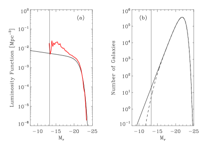
Figure 8.— (a) LF in the $r$-band for central galaxies, determined by Yang et al. (2009). The red line shows the LF by Blanton et al. (2005); it is the same as the red line in Fig. 4a, and has been included here for reference. (b) Number of galaxies per unit magnitude to be expected in the SDSS-DR7 spectroscopic survey for the LF in (a). The solid line shows the effect of the Malmquist bias, whereas the black dashed line also includes the incompleteness for low-SB objects.

4.2. Factors limiting the number of observed QXMPs

Assuming that our model for the selection function provides a good representation of the SDSS properties, one can investigate which, among the parameters of the survey, are responsible for the limited number of observed QXMPs. In principle, there are three main parameters that control such a number, namely, (1) the completeness, (2) the area coverage of the survey, and (3) the apparent magnitude limit.

The number of objects of a particular type in the survey linearly scales with the area of the survey. Since SDSS already covers a significant part of the sky (around 20 %; Abazajian et al. 2009), this is not a limiting factor in the present case. In other words, no dramatic (tenfold) increase in the number of QXMPs will follow from increasing the area covered by the SDSS-DR7.

Even though completeness is an important factor, it is not the key factor that determines $N_{\rm QXMP}$. At the absolute magnitude limit that characterizes the QXMPs, the completeness is around 30 % (see Fig. 5). Although the completeness can be increased, it cannot exceed the value of one, which in turn implies a moderate increase in $N_{\rm QXMP}$. This dependence can be apprised in Fig. 9a, where the expected number of QXMPs is represented for different SB cutoffs of the completeness function. To compute the number, we have used the same completeness of the SDSS-DR7 (Fig. 5, the red solid line), shifted in $SB_{r}$, with the shift parameterized as the one-half completeness $SB_{r}$. As the SB of the drop increases, $N_{\rm QXMP}$ increases too. However, it saturates at a value that is only ten times larger than the value corresponding to the SDSS-DR7 spectroscopic survey (the point of lower SB in Fig. 9a). The curves in Fig. 9a and 9b assume the LF shown as a red solid line in Fig. 6a.

The apparent magnitude limit turns out to be the critical parameter that limits the number of QXMPs. It determines the volume sampled by the survey, which, in principle, can be increased indefinitely as $m_{limit}$ increases. The behavior is shown in Fig. 9b. Just to provide an idea of the increase, if one consideres the apparent magnitude limit of the SDSS-DR7 photometric survey ($m_{limit}=22.2$ in the $r-$band), then Fig. 9b predicts the presence of approximately 2800 QXMPs, which should be compared to the prediction of 6 QXMPs in the SDSS-DR7 spectroscopic sample ($m_{limit}=17.77$; see Table 2 and Fig. 9b).

Figure 9.— (a) Number of QXMPs expected when the SB cutoff of the completeness function changes. The cutoff is quantified as the SB having a completeness of one half. It only has a moderate impact on $N_{\rm QXMP}$. (b) Number of QXMPs expected in the SDSS-DR7 spectroscopic survey if the apparent magnitude limit, $m_{lim}$, could be modified. This parameter critically determines $N_{\rm QXMP}$. The range of the ordinates in (a) and (b) is the same.

4.3. Number of QXMPs in other surveys

The formalism developed in Sect. 3 allows us to estimate the number of expected QXMPs in any magnitude-limited survey, provided their magnitude limit, half-completeness, $SB_{r}$, and coverage area. If the completeness function is assumed to have the functional form of the SDSS completeness, then the half-completeness, $SB_{r}$, fully describes it. We carried out the exercise of estimating $N_{\rm QXMP}$ for a number of ongoing and forthcoming large area surveys, specifically, for the the Dark Energy Survey (DES; The DES Collaboration 2005), the Galaxy and Mass Assembly survey (GAMA; Liske et al. 2015), the Kilo-Degree Survey (KIDS; de Jong et al. 2015), and the Large Synoptic Survey Telescope (LSST; Ivezic et al. 2008).

Table 3$N_{\rm QXMP}$ for various ongoing and forthcoming galaxy surveys

Survey	$r$-band $m_{lim}$	Half-Completeness SB	Area	$N_{\rm QXMP}\,^{a}$	$N_{\rm QXMP}\,^{b}$
	[mag]	[mag arcsec-2]	[deg2]
SDSS$\,{}^{c}$ spectroscopic	17.8	23.4	8032	42	6
GAMA$\,{}^{d}$	19.8	26.0	286	83	11
SDSS$\,{}^{c}$ photometric	22.2	23.4	8423	2.0$\times 10^{4}$	2.8$\times 10^{3}$
KIDSe	24.0	27.2	1500	1.5$\times 10^{5}$	2.0$\times 10^{4}$
DES$\,{}^{f}$	24.1	27.1	5000	5.8$\times 10^{5}$	7.6$\times 10^{4}$
LSST$\,{}^{g}$, single visit	24.7	25.9	18000	4.3$\times 10^{6}$	6.0$\times 10^{5}$
LSST$\,{}^{g}$, co-added 10 year	27.5	28.7	18000	2.3$\times 10^{8}$	3.0$\times 10^{7}$

a Assuming a LF function growing with increasing magnitude (the black solid line in Fig. 6a).

b Assuming a LF function decreasing with increasing magnitude (the red solid line in Fig. 6a).

c For DR7. Parameters from the webpage: http://classic.sdss.org/dr7/.

d Galaxy and Mass Assembly. Parameters from Liske et al. (2015).

e Kilo-Degree Survey. Parameters from de Jong et al. (2015)

f Dark Energy Survey, after 5 years. Parameters from The DES Collaboration (2005).

g Large Synoptic Survey Telescope. Parameters from Ivezic et al. (2008).

The parameters that define the surveys are given in Table 3. LSST, DES and KIDS do not explicitly give the half-compleness, SB. In these cases, we infer it from the depth for point sources as described in Appendix B.

As is shown in Table 3, the number of QXMPs expected in the next generation of wide area surveys is very large, reaching up to $10^{7}$ in the 10-year average LSST. The actual number changes by one order of magnitude, depending on whether the LF increases towards low luminosity (the black solid line in Fig. 6a) or if it flattens out (the red solid line in Fig. 6a). Therefore, it should be easy to discriminate both trends using these new surveys. For example, the ongoing GAMA survey predicts 10 or 100 QXMPs, depending on the LF faint end. In agreement with the conclusion in the previous section, the key factor determining $N_{\rm QXMP}$ is not so much the SB cutoff but the limiting magnitude, $m_{lim}$. Note, however, that even if the surveys contain all these new QXMPs, it will be imposible to confirm the XMP nature of many of the faint objects. The spectroscopic follow up required to determine abundances will be possible only in those QXMPs where star-forming regions are bright enough.

5. Conclusions

Galaxies follow a relationship between luminosity and gas-phase metallicity, so that faint galaxies tend to be metal-poor galaxies as well. Since the luminosity function increases steeply towards low luminosity, one would naively expect that most observed galaxies are metal-poor. This is not the case. This apparent inconsistency is usually attributed to the low-luminosity of the metal-poor objects, which are under-represented in galaxy surveys. Firstly, this occurs due to the Malmquist bias: surveys are apparent magnitude-limited, so that the sampled volume drops down dramatically for faint sources. Secondly, low-luminosity galaxies are also low-SB galaxies, and the surveys tend to miss extended, low-SB objects.

This dearth of metal-poor galaxies is particularly severe for the so-called extremely metal poor (XMP) galaxies, with a gas-phase metallicity smaller than a tenth of the solar metallicity. They are of astrophysical interest for a number of reasons highlighted in Sect. 1, but they represent only a tiny fraction of the galaxies in the most popular surveys (e.g., 0.02 % in the recent SDSS-DR7 search by Sánchez Almeida et al. 2016). Moreover, most of the observed XMPs are outliers of the luminosity-metallicity relationship. Therefore, they are not part of the predicted sea of faint XMPs. (We denote the faint XMPs as quiescent XMPs or QXMPs.) The question arises as to whether the actual number of observed XMPs is quantitatively consistent with the expected number. We address this question in the present paper. Most known XMPs come from the SDSS-DR7 spectroscopic survey, so we compare the number of observed QXMPs in this survey with the expected number. The main conclusion of our work is that they disagree, unless the luminosity function for QXMPs is considerably shallower than the extrapolation to low luminosity of the observed LF.

The number of QXMPs in the SDSS-DR7 spectroscopic survey turns out to be $9\pm 3$, with the error bar representing the Poissonian fluctuation (Sect. 2, Table 1, and Figs. 1 and 2). Extrapolating to $M_{r}>-13.3$ the LF for faint galaxies observed by Blanton et al. (2005, shown in Fig. 4a), the expected number is 42 (Sect. 3). This estimate takes into account the Malmquist bias plus the finite completeness of SDSS for low-SB objects. In addition, it includes the scatter in the SB versus magnitude relationship, that effectively increases the completeness of the survey at low luminosities (Appendix). Once the various uncertainties involved in the estimate are considered (Sect. 3.2), the expected number of QXMPs is in the range between 12 and 73, with the low value highly disfavored.

On the other hand, if the previous LF is modified to include the decrease of baryon fraction in low-mass dark matter halos, then the upturn at low luminosity disappears (Fig. 6a), rendering an expectation of only 6 QXMPs. (The number is between 3 and 12 when uncertainties are taken into account; see Sect. 3.3.) The tension with observation automatically disappears. Including the varying baryon fraction implicitly assumes the QXMPs to be central galaxies in their dark matter haloes. In fact, the LF for centrals determined by Yang et al. (2009, see Fig. 8a) does not show the upturn, and it predicts between 3 and 9 QXMPs (Sect. 4.1 and Table 2). The agreement with observations has several implications. Firstly, QXMPs seem to be centrals, rather than satellite galaxies. QXMPs become tracers of low-mass halos not gravitationally bound to more massive halos, and so they can be used to trace these haloes observationally. These low-mass dark matter halos are of clear astrophysical interest in the context of characterizing the building blocks in the hierarchical formation of galaxies and, in particular, the effect of the cosmic UV background in their baryonic content. The fact that QXMPs seem to be centrals is consistent with the observation that most XMPs appear to be isolated and in low density regions of the Universe (e.g., Filho et al. 2015; Sánchez Almeida et al. 2016). Secondly, the upturn in the faint end of the observed LF appears to be due to satellite galaxies, and this should be taken into account when comparing observations and numerical models. Thirdly, the baryon fraction predicted by the numerical models by Okamoto et al. (2008) is consistent with observations. Finally, there is no expectation of finding a significant number of new QXMPs in the SDSS-DR7 spectroscopic survey.

Assuming that our modeling of the SDSS biases is correct, we have studied which, among the parameters defining the survey, restricts the number of QXMPs most (Sect. 4.2). It turns out to be the apparent magnitude limit, which is more relevant than the incompleteness. Thus, the photometric SDSS-DR7 survey, which is 4 magnitudes deeper than the spectroscopic one, should contain as many as 2800 QXMPs. The expected numbers in various other surveys are determined in Sect. 4.3, and a summary is presented in Table 3. Future surveys are predicted to detect QXMPs in large quantities.

Appendix A Scatter in the $SB$ versus $M$ relationship

Equation (11) assumes a one-to-one correspondence between the SB and the absolute magnitude of the source. The fact that most observed QXMPs are high-SB outliers of the $SB$ versus $M$ relationship indicates that the scatter in this relationship may be of importance in our estimate. In simple terms, an object is preferentially picked out by SDSS if it is of high SB for its absolute magnitude.

In order to treat this case in our formalism, we assume the LF to be the marginal probability density (see, e.g., Martin 1971) of a bi-variate joint probability density function (PDF), $P(M,SB)$, that quantifies the number of galaxies with absolute magnitude $M$ and surface brightness $SB$, i.e.,

$$\Phi(M)=\int_{\forall\,SB}P(M,SB)\,dSB.$$ (A1)

Then computing the number is equivalent to Eq. (6), but it involves a double integral over $M$ and $SB$,

$$N(M>M_{lim})=\int^{M_{1}}_{M_{lim}}\int_{\forall SB}\,P(M,SB)\,V(M)\,C^{\prime}(SB)\,dSB\,dM,$$ (A2)

with the symbol $C^{\prime}$ standing for the completeness function expressed in terms of the surface brightness. The bi-variate distribution function can be expressed in terms of the conditional probability function, $P(SB|M)$ (the probability of having a surface brightness $SB$, given that the absolute magnitude is $M$),

$$P(M,SB)=P(SB|M)\,\Phi(M).$$ (A3)

Inserting the expression (A3) into Eq. (A2) one recovers Eqs. (6) and (11), provided that $C(M)$ is replaced with an effective completeness function, $C_{eff}$, given by

$$C_{eff}(M)=\int_{\forall\,SB}P(SB|M)\,C^{\prime}(SB)\,dSB.$$ (A4)

With minimal assumptions, one can write down the conditional probability density function as

$$P(SB|M)={{1}\over{\Delta_{0}}}\,G({{SB-SB_{0}}\over{\Delta_{0}}}),$$ (A5)

with

$$SB_{0}=SB_{0}(M),$$

$$\Delta_{0}=\Delta_{0}(M),$$

and $G$ any positive function properly normalized,

$$\int_{-\infty}^{+\infty}G(x)\,dx=1.$$ (A6)

The case without scatter in the SB versus M relationship corresponds to an infinitely narrow conditional probability function, which we can easily treat in the limit $\Delta_{0}\longrightarrow 0$, so that

$${{1}\over{\Delta_{0}}}\,G\big{(}{{SB-SB_{0}}\over{\Delta_{0}}}\big{)}\longrightarrow\delta(SB-SB_{0}),$$ (A7)

with $\delta$ a delta Dirac function. Inserting the previous expression into Eq. (A4) yields

$$C_{eff}(M)=C(M)=C^{\prime}(SB_{0}(M)),$$ (A8)

with $SB_{0}(M)$ given by expression (10). In general, the computation of $N_{\rm QXMP}$ must make use of the full expression, where the effective completeness function is a type of convolution of the completeness function with the conditional PDF. Following Blanton et al. (2005), we will assume that the conditional PDF is a Gaussian,

$$G(x)={{1}\over{\sqrt{2\pi}}}{\Large\exp}(-{{x^{2}}\over{2}}),$$ (A9)

with the mean, $SB_{0}$, and the variance, $\Delta^{2}_{0}(M)$, measured to be

$$SB_{0}(M)=23.8+0.45\,(M+13.3),$$ (A10)

$$\Delta_{0}(M)=1.16+0.081\,(M+13.3).$$

Equation (A10) is identical to Eq. (10), and has been included here for comprehensiveness. The effective completeness function resulting from $C^{\prime}$ in Blanton et al. (2005) and the above parametrization of the conditional function is shown as the red solid line in Fig. 5. The net effect is a significant enhancement of the completeness at low luminosity.

We note that in the limiting case when (1) $C^{\prime}(SB)$ is a Heaviside step function (zero for $SB$ larger than a given surface brightness, and one elsewhere), and when (2) $G$ is a Gaussian of constant width $\Delta_{0}$, then $C_{eff}$ in Eq. (A4) has the shape of an erf function. This approximation is used in the main text.

Appendix B Estimate of the SB limit from the depth of the survey

In order to predict the number of QXMPs expected in various surveys, one needs to assign a SB limit to them. The requirements of the survey are often set in terms of the depth for point sources, i.e., the flux that a point source must have to grant detection with a signal-to-noise ratio a number of times above the noise level. In order to transform this parameter to the corresponding SB limit, we proceed as follows: the depth for point sources, $m_{\rm point}$, is defined as,

$$m_{\rm point}=-2.5\,\log(\xi\,\sigma\sqrt{n_{\rm point}})+\kappa,$$ (B1)

where $\sigma$ stands for the noise per pixel, $\xi$ for the level above noise to grant detection, and $n_{\rm point}$ for the number of pixels covered by a point source. $\kappa$ sets the zero of the magnitude scale. Equation (B1) assumes the noise of adjacent pixels to be independent, so that the noise of the sum of them adds up quadratically. We will define the SB limit as the SB of an extended source exceeding the noise in one arcsec, i.e.,

$$m_{\rm ext}=-2.5\,\log(\sigma\sqrt{n_{\rm 1^{\prime\prime}}})+\kappa,$$ (B2)

with $n_{\rm 1^{\prime\prime}}$ for the number of pixels in one arcsec. Since

$$n_{\rm point}/n_{\rm 1^{\prime\prime}}=\pi\,{\rm(FWHM/2)^{2}},$$ (B3)

with FWHM the full width half-maximum of the point-spread funcion in arcsec, then Eqs. (B1) and (B2) lead to,

$$m_{\rm ext}=m_{\rm point}+2.5\log(\xi{{\sqrt{\pi}}\over{2}}{\rm FWHM}).$$ (B4)

Equation (B4) links the depth, $m_{\rm point}$, with the SB limit, $m_{\rm ext}$.

References

- Abazajian et al. (2009) Abazajian, K. N., Adelman-McCarthy, J. K., Agüeros, M. A., et al. 2009, ApJS, 182, 543
- Asplund et al. (2009) Asplund, M., Grevesse, N., Sauval, A. J., & Scott, P. 2009, ARA&A, 47, 481
- Benson (2010) Benson, A. J. 2010, Phys. Rep., 495, 33
- Berg et al. (2012) Berg, D. A., Skillman, E. D., Marble, A. R., et al. 2012, ApJ, 754, 98
- Binggeli et al. (1988) Binggeli, B., Sandage, A., & Tammann, G. A. 1988, ARA&A, 26, 509
- Blanton et al. (2005) Blanton, M. R., Lupton, R. H., Schlegel, D. J., et al. 2005, ApJ, 631, 208
- Blanton & Moustakas (2009) Blanton, M. R. & Moustakas, J. 2009, ARA&A, 47, 159
- Ceverino et al. (2016) Ceverino, D., Sánchez Almeida, J., Muñoz Tuñón, C., et al. 2016, MNRAS, 457, 2605
- Christensen et al. (2016) Christensen, C. R., Davé, R., Governato, F., et al. 2016, ApJ, 824, 57
- Combes (2004) Combes, F. 2004, in IAU Symposium, Vol. 217, Recycling Intergalactic and Interstellar Matter, ed. P.-A. Duc, J. Braine, & E. Brinks, 440
- Cyburt et al. (2016) Cyburt, R. H., Fields, B. D., Olive, K. A., & Yeh, T.-H. 2016, Reviews of Modern Physics, 88, 015004
- Dalla Vecchia & Schaye (2008) Dalla Vecchia, C. & Schaye, J. 2008, MNRAS, 387, 1431
- Davé et al. (2012) Davé, R., Finlator, K., & Oppenheimer, B. D. 2012, MNRAS, 421, 98
- de Jong et al. (2015) de Jong, J. T. A., Verdoes Kleijn, G. A., Boxhoorn, D. R., et al. 2015, A&A, 582, A62
- Efstathiou (1992) Efstathiou, G. 1992, MNRAS, 256, 43P
- Elmegreen et al. (2013) Elmegreen, B. G., Elmegreen, D. M., Sánchez Almeida, J., et al. 2013, ApJ, 774, 86
- Elmegreen & Hunter (2015) Elmegreen, B. G. & Hunter, D. A. 2015, ApJ, 805, 145
- Elmegreen et al. (2012) Elmegreen, D. M., Elmegreen, B. G., Sánchez Almeida, J., et al. 2012, ApJ, 750, 95
- Filho et al. (2016) Filho, M. E., Sánchez Almeida, J., Amorín, R., et al. 2016, ApJ, 820, 109
- Filho et al. (2015) Filho, M. E., Sánchez Almeida, J., Muñoz-Tuñón, C., et al. 2015, ApJ, 802, 82
- Fisher et al. (2014) Fisher, D. B., Bolatto, A. D., Herrera-Camus, R., et al. 2014, Nature, 505, 186
- Geller et al. (2012) Geller, M. J., Diaferio, A., Kurtz, M. J., Dell’Antonio, I. P., & Fabricant, D. G. 2012, AJ, 143, 102
- Gnedin (2000) Gnedin, N. Y. 2000, ApJ, 542, 535
- Governato et al. (2010) Governato, F., Brook, C., Mayer, L., et al. 2010, Nature, 463, 203
- Guseva et al. (2015) Guseva, N. G., Izotov, Y. I., Fricke, K. J., & Henkel, C. 2015, A&A, 579, A11
- Guseva et al. (2009) Guseva, N. G., Papaderos, P., Meyer, H. T., Izotov, Y. I., & Fricke, K. J. 2009, A&A, 505, 63
- Hirschauer et al. (2016) Hirschauer, A. S., Salzer, J. J., Skillman, E. D., et al. 2016, ApJ, 822, 108
- Ivezic et al. (2008) Ivezic, Z., Tyson, J. A., Abel, B., et al. 2008, ArXiv e-prints
- Izotov et al. (2004) Izotov, Y. I., Stasińska, G., Guseva, N. G., & Thuan, T. X. 2004, A&A, 415, 87
- Izotov et al. (2006) Izotov, Y. I., Stasińska, G., Meynet, G., Guseva, N. G., & Thuan, T. X. 2006, A&A, 448, 955
- Izotov & Thuan (2007) Izotov, Y. I. & Thuan, T. X. 2007, ApJ, 665, 1115
- Izotov et al. (2012) Izotov, Y. I., Thuan, T. X., & Guseva, N. G. 2012, A&A, 546, A122
- James et al. (2015) James, B. L., Koposov, S., Stark, D. P., et al. 2015, MNRAS, 448, 2687
- Jester et al. (2005) Jester, S., Schneider, D. P., Richards, G. T., et al. 2005, AJ, 130, 873