Non-linear quantum dynamics in strong and short electromagnetic fields

Abstract

In our contribution we give a brief overview of two widely discussed quantum processes: electron-positron pairs production off a probe photon propagating through a polarized short-pulsed electromagnetic (e.m.) (e.g. laser) wave field or generalized Breit-Wheeler process and a single a photon emission off an electron interacting with the laser pules, so-called non-linear Compton scattering. We show that at small and moderate laser field intensities the shape and duration of the pulse are very important for the probability of considered processes. However, at high intensities the multi-photon interactions of the fermions with laser field are decisive and completely determined all aspects of subthreshold $e^{+}e^{-}$ pairs and photon production.

1 Introduction

The rapidly progressing laser technology [1] offers unprecedented opportunities for investigations of quantum systems with intense laser beams [2]. A laser intensity $I_{L}$ of $\sim 2\times 10^{22}$ W/cm² has been already achieved [3]. Intensities of the order of $I_{L}\sim 10^{23}...10^{25}$ W/cm² are envisaged in near future, e.g. at the CLF [4], ELI [5], HiPER [6]. Further facilities are in planning on construction stage, e.g. PEARL laser facility [7] at Sarov/Nizhny Novgorod, Russia. The high intensities are provided in short pulses on a femtosecond pulse duration level [2, 8, 9], with only a few oscillations of the electromagnetic (e.m.) field or even sub-cycle pulses. (The tight connection of high intensity and short pulse duration is further emphasized in [10]. The attosecond regime will become accessible at shorter wavelengths [11, 12]).

Quantum processes occurring in the interactions of charge fermions in very (infinitely) long e.m. pulse were investigated in detail in the pioneering works of Reiss [13] as well as Narozhny, Nikishov and Ritus [14, 15, 16]. We call the such approaches as an infinite pulse approximation (IPA) since it refers to a stationary scattering process. Many simple and clear expressions for the production probabilities and cross sections have been obtain within IPA. It was shown that the charged fermion (electron, for instance) can interact with $n\geq 1$ photon simultaneously ($n$ is an integer number),

However, recently it has become clear that for the photon production off an electron interacting with short laser pulse (Compton scattering) and for $e^{+}e^{-}$ pair production off a probe photon interacting with short e.m. pulses (Breit-Wheeler process) the finite pulse shape and the pulse duration become important (see, for example [17] and reference their in). That means the treatment of the intense and short laser field as an infinitely long wave train is no longer adequate. The theory must operate with essentially finite pulse. We call such approaches as a finite pulse approximation (FPA).

In this contribution we consider some particularities of generalized Breit-Wheeler and Compton processes in a short and strong laser pulses. For this purpose we use the widely employed the four electromagnetic (e.m.) potential for a circularly polarized laser field in the axial gauge $A^{\mu}=(0,\,\mathbf{A}(\phi))$ with

$$\mathbf{A}(\phi)=f(\phi)\left(\mathbf{a}_{1}\cos(\phi+\tilde{\phi})+\mathbf{a}_{2}\sin(\phi+\tilde{\phi})\right)~{},$$ (1)

where $\phi=k\cdot x$ is invariant phase with four-wave vector $k=(\omega,\mathbf{k})$, obeying the null field property $k^{2}=k\cdot k=0$ (a dot between four-vectors indicates the Lorentz scalar product) implying $\omega=|\mathbf{k}|$, $\mathbf{a}_{(1,2)}\equiv\mathbf{a}_{(x,y)}$; $|\mathbf{a}_{x}|^{2}=|\mathbf{a}_{y}|^{2}=a^{2}$, $\mathbf{a}_{x}\mathbf{a}_{y}=0$; transversality means $\mathbf{k}\mathbf{a}_{x,y}=0$ in the present gauge. The envelope function $f(\phi)$ with $\lim\limits_{\phi\to\pm\infty}f(\phi)=0$ accounts for the finite pulse length. We are going to analyze dependence of observables on the shape of $f(\phi)$ in Eq. (1) for two types of envelopes: the one-parameter hyperbolic secant (hs) shape and the two-parameter symmetrized Fermi (sF) shape widely used for parametrization of the nuclear density [Luk]: $f_{\rm hs}(\phi)=(\cosh\phi/{\Delta})^{-1}$ and $f_{\rm sF}(\phi)=(\cosh{\Delta}/{b}+1)(\cosh{\Delta}/{b}+\cosh{{\phi}/{b}})^{-1}$. The parameter $\Delta$ characterizes the pulse duration $2\Delta$ with $\Delta=\pi N$, where $N$ has a meaning of a ”number of oscillations”  in the pulse. The parameter $b$ in the sF shape describes the ramping time in the neighborhood of $\phi\sim\Delta$. Small values of ratio $b/\Delta$ cause a flat-top shaping. At $b/\Delta\to 0$, the sF shape becomes a rectangular pulse. In the following, we choose the ratio $b/\Delta$ as the second independent parameter for the sF envelope function. These two shapes cover a variety of relevant envelopes discussed in literature (for details see [18]). The carrier envelope phase $\tilde{\phi}$ is particularly important for the short the pulse duration with $N\leq 1$. Therefore we start our presentation with case of $\tilde{\phi}=0$ and discuss impact of finite carrier phase at the end. Finally we note that, the interaction of the background field is determined by dimensionless reduced e.m. intensity $\xi^{2}=\sqrt{-A^{2}}/M_{e}^{2}$, where $M_{e}$ is the electron mass (we use natural units with $c=\hbar=1$, $e^{2}/4\pi=\alpha\approx 1/137.036$). (for more detail see [17]).

Some important difference between IPA and FPA is that in the first case the variable $n=1,2,\,\cdots$ is integer, it refers to the contribution of the individual harmonics. The value $n\omega$ is related to the energy of the background field involved into considered quantum process. Obviously, this value is a multiple of $\omega$. In FPA, the basic subprocess operate with $l$ background photons, where $l$ is a continuous variable. The quantity $l\omega$ can be considered as the energy partition of the laser beam involved into considered process, and it is not a multiple $\omega$. Mindful of this fact, without loss of generality, we denote the processes with $l>1$ as a generalized multi-photon processes, remembering that $l$ is a continuous quantity.

This lecture is based on the review paper [17] and is organized as follows. Sect. 2 is devoted to the non-linear Breit-Wheeler process. In Sect. 3 we discuss several aspects of non-linear Compton scattering for short and sub-cycle pulses. Our conclusions are presented in Sect. 5.

2 The ${\mathbf{e^{+}e^{-}}}$ pair production in a finite pulse

We consider $e^{+}e^{-}$ pair production in the interaction of a probe photon with a circularly polarized e.m.field (1 within the Furry picture, which diagrammatically is represented by a one-vertex graph, describing the decay of the probe photon with the four-momentum $k^{\prime}$ into a laser dressed $e^{+}e^{-}$ pair. The presence of the background e.m. field is included in the Volkov solution of the outgoing $e^{+}$ and $e^{-}$. (In the weak-field approximation this graph turns into the known two two-vertex graphs for the perturbative Breit-Wheeler process). Contrary to the IPA, utilization of (1) the Volkov solutions in FPA assume all fermion momenta and masses take their vacuum values $p$ and $m$, respectively, whereas the corresponding wave functions are modified in accordance with the Volkov solution [19, 20] (with more complicated compare to IPA, phase factor). The finite (in space-time) e.m. potential (1) for FPA requires the use of Fourier integrals for invariant amplitudes, instead of Fourier series which are employed in IPA. The partial harmonics become thus continuously in FPA. The $S$ matrix element is expressed generically as

$$S_{fi}=\frac{-ie}{\sqrt{2p_{0}2p_{0}^{\prime}2\omega^{\prime}}}\int\limits_{\zeta}^{\infty}dl\,M_{fi}(l)(2\pi)^{4}\delta^{4}(k^{\prime}+lk-p-p^{\prime}),$$ (2)

where $k$, $k^{\prime}$, $p$ and $p^{\prime}$ refer to the four-momenta of the background (laser) field (1), incoming probe photon, outgoing positron and electron, respectively, the low limit $\zeta$ is defined in Eq. (LABEL:I-zeta). The transition matrix $M_{fi}(l)$ consists of four terms

$$\,M_{fi}(l)=\sum\limits_{i=0}^{3}M^{(i)}\,C^{(i)}(l)~{},$$ (3)

where transition matrices $M^{i}$ are determined by the Dirac structure in the amplitude (2) (cf. [17]), whereas the non-linear dynamics of pair production is determined by the functions $C^{i}(l)$ expressed trough the basic functions $Y_{l}$, $X_{l}$ which are an analog of the Bessel functions

$$C^{(0)}(l)=\widetilde{Y}_{l}(z){\rm e}^{il\phi_{0}},\,\,\widetilde{Y}_{l}(z)=\frac{z}{2l}\left(Y_{l+1}(z)+Y_{l-1}(z)\right)-\xi^{2}\frac{u}{u_{l}}\,X_{l}(z)^{\prime}\,\,C^{(1)}(l)=X_{l}(z)\,{\rm e}^{il\phi_{0}},$$

$$C^{(2)}(l)=\frac{1}{2}\left(Y_{l+1}{\rm e}^{i(l+1)\phi_{0}}+Y_{l-1}{\rm e}^{i(l-1)\phi_{0}}\right),\,\,C^{(3)}(l)=\frac{1}{2i}\left(Y_{l+1}{\rm e}^{i(l+1)\phi_{0}}-Y_{l-1}{\rm e}^{i(l-1)\phi_{0}}\right)~{}$$ (4)

with

$$Y_{l}(z)=\frac{1}{2\pi}{\rm e}^{-il\phi_{0}}\int\limits_{-\infty}^{\infty}\,d\phi\,{f}(\phi)\,{\rm e}^{il\phi-i{\cal P}(\phi)}~{},\,\,X_{l}(z)=\frac{1}{2\pi}{\rm e}^{-il\phi_{0}}\int\limits_{-\infty}^{\infty}\,d\phi\,{f^{2}}(\phi)\,{\rm e}^{il\phi-i{\cal P}(\phi)}~{},\$$ (5)

$${\cal P(\phi)}=z\int\limits_{-\infty}^{\phi}\,d\phi^{\prime}\,\cos(\phi^{\prime}-\phi_{0}+\tilde{\phi})f(\phi^{\prime})-\xi^{2}\zeta u\int\limits_{-\infty}^{\phi}\,d\phi^{\prime}\,f^{2}(\phi^{\prime})~{}.$$ (6)

The quantity $z$ is related to $\xi$, $l$, and $u\equiv(k^{\prime}\cdot k)^{2}/\left(4(k\cdot p)(k\cdot p^{\prime})\right)$ via $z=2l\xi\sqrt{\frac{u}{u_{l}}\left(1-\frac{u}{u_{l}}\right)}$; with $u_{l}\equiv l/\zeta$. The phase $\phi_{0}$ is equal to the azimuthal angle of the direction of flight of the outgoing electron in the $e^{+}e^{-}$ pair rest frame $\phi_{0}=\phi_{p^{\prime}}\equiv\phi_{e}$. The quantity

$$\zeta=\frac{4M_{e}^{2}}{s}$$ (7)

is important variable for the generalized Breit-Wheeler process: $\zeta>1$ or $\zeta<1$ correspond to the above- and subthreshold- pair production, respectively. The later one is mainly described by by the multi-photon interactions.

The production probability is presented as the integral over the variables $\phi_{e}$, $u$ and $l$

$$W=\frac{\alpha m\zeta^{1/2}}{16\pi N_{0}}\int\limits_{0}^{2\pi_{e}}d\phi_{e}\int\limits_{1}^{\frac{l}{\zeta}}\frac{du}{u^{3/2}\sqrt{u-1}}\,\int\limits_{\zeta}^{\infty}\,dl\ w{(l)}$$ (8)

with $N_{0}\simeq N$ and the partial probability

$$w(l)=2\widetilde{Y}^{2}_{l}(z)+\xi^{2}(2u-1)\left(Y^{2}_{l-1}(z)+Y^{2}_{l+1}(z)-2\widetilde{Y}_{l}(z)X^{*}_{l}(z)\right)~{}.$$ (9)

2.1 Pair production at small field intensities ($\xi^{2}\ll 1$)

In case of small $\xi^{2}\ll 1$, implying $z<1$, we decompose $l=n+\epsilon$, where $n$ is the integer part of $l$, yielding

$$Y_{l} \simeq \frac{1}{2\pi}\int\limits_{-\infty}^{\infty}\,d\psi\,{\rm e}^{il\psi-iz\sin\psi\,f(\psi+\phi_{0})}f(\psi+\phi_{0})$$ (10)

$$= \frac{1}{2\pi}\int\limits_{-\infty}^{\infty}\,d\psi\sum\limits_{m=0}^{\infty}\frac{(iz)^{m}}{m!}\sin^{m}\psi\,{\rm e}^{i(n+\epsilon)\psi}f^{m+1}(\psi+\phi_{0})~{}.$$

Similarly, for the function $X_{l}(z)$ the substitution $f^{m+1}\to f^{m+2}$ applies. The dominant contribution to the integral in (10) with rapidly oscillating integrand comes from the term with $m=n$, which results in

$$Y_{n+\epsilon}\simeq\frac{z^{n}}{2^{n}n!}\,{\rm e}^{-i\epsilon\phi_{0}}F^{(n+1)}(\epsilon)~{},\qquad X_{n+\epsilon}\simeq\frac{z^{n}}{2^{n}n!}\,{\rm e}^{-i\epsilon\phi_{0}}F^{(n+2)}(\epsilon)~{},$$ (11)

where the function $F^{(n)}(\epsilon)$ is the Fourier transform of the function $f^{n}(\psi)$.

As an example, let us analyze the $e^{+}e^{-}$ production near the threshold, i.e. $\zeta\sim 1$. In this case, the contribution with $n=1$ is dominant and, therefore, the functions $Y_{0+\epsilon}$ are crucial, including the first term in (9). The functions $X_{0+\epsilon}$ are not important because they are multiplied by the small $\xi^{2}$ and may be omitted. Negative $\epsilon=\zeta-1$ and positive $\epsilon$ correspond to the above- and sub-threshold pair production, respectively. The function $Y_{0+\epsilon}$ reads $Y_{0+\epsilon}=F^{(1)}(\epsilon)\,\exp[-i\phi_{0}\epsilon]$, where the Fourier transforms $F^{(1)}(x)$ for the hs and sF envelope decrease as a function of $l$ in a different way $F_{\rm hs}(l)\sim\exp[-\frac{1}{2}\Delta l]$ and $F_{\rm sF}(l)\sim[-\pi bl]$ which is manifested in the spectra of $e^{+}e^{-}$ pair production. The $\phi_{0}$ dependence of the production probability disappears in this case because the latter one is determined by the quadratic terms of the $Y$ functions. As we have seen the Fourier transform of the envelope function plays important role in shape and absolute value of the production probability. As an example, in Fig. 1 we show the total probability $W$ of $e^{+}e^{-}$ emission as a function of the sub-threshold parameter $\zeta$ in the vicinity $\zeta\sim 1$.

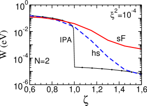
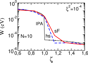
Figure 1: The total probability $W$ of the $e^{+}e^{-}$ pair production as a function of $\zeta$ for short pulses with $\Delta=\pi N$ for $N=2$, and 10 shown in the left and right panels, respectively; $\xi^{2}=10^{-4}$. The dashed and solid curves correspond to the hyperbolic secant and symmetrized Fermi envelope shapes with $b/Delta=0.1$, respectively. The thin solid curves marked by dots depict the IPA result.

The dashed and solid curves correspond to the hyperbolic secant and symmetrized Fermi envelope shapes, respectively. The left and right panels correspond to the short pulses with $\Delta=\pi N$ for $N=2$, and 10, respectively, at $\xi^{2}=10^{-4}$. For comparison, we present also the IPA results. Naturally, that in the above-threshold region, results of IPA and FPA are equal to each other. However, in the sub-threshold region, where $\zeta$ is close to integer numbers, the probability of FPA considerably exceeds (by more than two orders of magnitude) the corresponding IPA result. In the case of the hyperbolic secant envelope function, the probability increases with decreasing pulse duration. The results of FPA and IPA become comparable at $N\geq 10$. Qualitatively, this result is also valid for the case of the symmetrized Fermi distribution. However, in this case the enhancement of the probability in FPA is much greater. Other important details may be found in [18].

2.2 Effect of the finite carrier phase

It is naturally to expect that the effect of the finite carrier phase and appears in the azimuthal angle distribution of the outgoing electron (positron) in case of finite $\xi\sim 1$ and smooth envelope function with $N<1$, because at this conditions the functions $C^{i}$ are greatly enhanced [21]. As an example, in Fig. 2 (left panels) we show the differential cross section $d\sigma/d\phi_{e}$ of $e^{+}e^{-}$ pair production as a function of the azimuthal angle $\phi_{e}$ for different values of the carrier envelope phase $\tilde{\phi}$ and for pulse durations $\Delta=N\pi$ with $N=$ 1, and for $\xi^{2}=0.5$. The calculation is done for the essentially multi-photon region with $\zeta=4$.

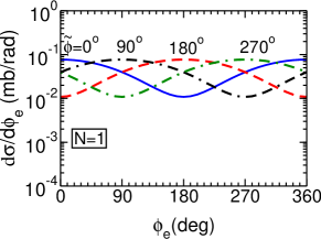
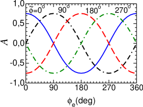
Figure 2: (Color online) Left column: The differential cross section as a function of the azimuthal angle of the direction of flight of the outgoing electron $\phi_{e}$, for different values of the carrier phase $\tilde{\phi}$ and for $N=1$. The solid, dash-dash-dotted, dashed and dash-dotted curves are for the CEP equal to 0, 90, 180 and 270 degrees, respectively. Right column: The anisotropy (12) for different values of $\tilde{\phi}$ as in left column. For $\xi^{2}=0.5$ and $\zeta=4$.

The corresponding anisotropy of the electron (positron) emission defined as

$${\cal A}=\frac{d\sigma(\phi_{e})-d\sigma(\phi_{e}+\pi)}{d\sigma(\phi_{e})+d\sigma(\phi_{e}+\pi)}~{},$$ (12)

are exhibited in Fig. 2 (right panels). One can see a strong dependence of the anisotropy as a function of CEP. The increase of the pulse duration leads to a decrease of the bump structure inn the differential cross sections and in absolute value of ${\cal A}$ and leads to the disappearance of the carrier phase effect.

2.3 Pair production at large field intensity $(\xi^{2}\gg 1)$

At large values of $\xi^{2}\gg 1$, the basic functions $Y_{l}$ and $X_{l}$ in Eq. (5) can be expressed as follows

$${Y}_{l}=\int\limits_{-\infty}^{\infty}dq\,F^{(1)}(q)\,G(l-q)~{},\qquad{X}_{l}=\int\limits_{-\infty}^{\infty}dq\,F^{(2)}(q)\,G(l-q)~{},$$ (13)

where $F^{(1)}(q)$ and $F^{(2)}(q)$ are Fourier transforms of the functions $f(\phi)$ and $f^{2}(\phi)$, respectively, and $G(l)$ may be written as

$$G(l)=\frac{1}{2\pi}\int\limits_{-\infty}^{\infty}d\phi\,{\rm e}^{i\left(l\phi-z\sin\phi+\xi^{2}\zeta u\phi\right)}~{}.$$ (14)

In deriving this equation we have considered the following facts: (i) at large $\xi^{2}$ the probability is isotropic, therefore we put $\phi_{0}=0$, (ii) the dominant contribution to the rapidly oscillating exponent comes from the region $\phi\simeq 0$, where the difference of two large values $l\phi$ and $z\sin\phi$ is minimal, and therefore, one can decompose the last term in the function ${\cal P}(\phi)$ in (LABEL:III21) around $\phi=0$, and (iii) replace in exponent $f(\phi)$ by $f(0)=1$.

Equation (14) represent an asymptotic form of the Bessel functions $J_{\tilde{l}}(z)$ [22] with $\tilde{l}=l+\xi^{2}\zeta u$ at $\tilde{l}\gg 1$, $z\gg 1$, and therefore the following identities are valid

$$G(\tilde{l}-1)-G(\tilde{l}+1)=2G_{z}^{\prime}(\tilde{l}),\qquad G(\tilde{l}-1)+G(\tilde{l}+1)=2\frac{\tilde{l}}{z}G(\tilde{l})~{},$$ (15)

which allow to express the partial probability $w(\tilde{l})$ in (9) as a sum of the diagonal (relative to $\tilde{l}$) terms: $Y_{\tilde{l}}^{2}$, $Y_{\tilde{l}}X_{\tilde{l}}$, $X_{\tilde{l}}^{2}$ and $Y^{{}^{\prime}2}_{\tilde{l}}$. The integral over $\tilde{l}$ from the diagonal term can be expressed as

$$I_{YY}=\int\limits_{\tilde{l}_{0}}^{\infty}d{\tilde{l}}\,Y_{l}^{2}=\int dq\,dq^{\prime}F^{(1)}(q)\,F^{(1)}(q^{\prime})\int\limits_{\tilde{l}_{0}}^{\infty}d\tilde{l}G(\tilde{l}-q)G(\tilde{l}-q^{\prime})~{},$$ (16)

where $\tilde{l}_{0}=\zeta(1+\xi^{2}u$. Taking into account that for the rapidly oscillating $G$ functions $G(l-q)G(l-q^{\prime})\simeq\delta(q-q^{\prime})G^{2}(l-q)$ and $\langle q\rangle\ll\langle l\rangle\ \sim\xi^{2}$ one gets

$$I_{YY}=\frac{1}{2\pi}\int\limits_{-\infty}^{\infty}d\phi f^{2}(\phi)\int\limits_{\tilde{l}_{0}}^{\infty}d\tilde{l}G^{2}(\tilde{l})=N_{YY}\int\limits_{\tilde{l}_{0}}^{\infty}d\tilde{l}G^{2}(\tilde{l})~{}.$$ (17)

Similar expressions are valid for the other diagonal terms with own normalization factors. For the $X^{2}_{\tilde{l}}$ term it is $N_{XX}=\frac{1}{2\pi}\int\limits_{-\infty}^{\infty}d\phi f^{4}(\phi)$, and for $Y_{\tilde{l}}X_{\tilde{l}}$, $N_{YX}=\frac{1}{2\pi}\int\limits_{-\infty}^{\infty}d\phi f^{3}(\phi)$. At large $\xi^{2}$, the probability does not depend on the envelope shape, because only the central part of the envelope is important. Therefore, for simplicity, we choose the flat-top shape with $N_{YY}=N_{YX}=N_{XX}=N_{0}=\Delta/\pi$ which is valid for any smooth (at $\phi\simeq 0$) envelopes.

Making a change of the variable $l\to\tilde{l}=l+\xi^{2}\zeta u$ the variable $z$ takes the following form

$$z^{2}=4\xi^{2}\zeta^{2}\left(uu_{l}-u^{2}\right)=\frac{4\xi^{2}l_{0}^{2}}{1+\xi^{2}}\left(uu_{\tilde{l}}-u^{2}\right)$$ (18)

with $l_{0}=\zeta(1+\xi^{2})$ and $u_{\tilde{l}}\equiv{\tilde{l}}/{l_{0}}$, that is exactly the same as the variable $z$ in IPA with the substitution $l\to\tilde{l}$. All these transformations allow to express the total probability in a form similar to the probability in IPA for large values of $\xi^{2}$ and a large number of partial harmonics $n$, replacing the sum over $n$ by an integral over $n$ [16]

$$W = \frac{1}{2}{\alpha M_{e}\zeta^{1/2}}\int\limits_{l_{0}}^{\infty}d\tilde{l}\int\limits_{1}^{u_{\tilde{l}}}\frac{du}{u^{3/2}\sqrt{u-1}}\{J^{2}_{\tilde{l}}(z)$$ (19)

$$+ \xi^{2}(2u-1)[(\frac{{\tilde{l}}^{2}}{z^{2}}-1){J}^{2}_{\tilde{l}}(z)+{J^{\prime}}^{2}_{\tilde{l}}(z)]\}~{}.$$

Utilizing Watson’s representation [22] for the Bessel functions at $\tilde{l},\,z\gg 1$ and $\tilde{l}>z$, $J_{\tilde{l}}(z)=({{2\pi\tilde{l}\tanh\alpha}})^{-1/2}\exp[-\tilde{l}(\alpha-\tanh\alpha)]$ with $\cosh\alpha={\tilde{l}}/{z}$, and employing a saddle point approximation in the integration in (19) we find the total probability of $e^{+}e^{-}$ production as (for details see Appendix A of [17])

$$W=\frac{3}{8}\sqrt{\frac{3}{2}}\frac{\alpha M_{e}\xi}{\zeta^{1/2}}\,d\,\exp\left[-\frac{4\zeta}{3\xi}(1-\frac{1}{15\xi^{2}})\right],\,\,d=1+\frac{\xi}{6\zeta}\left(1+\frac{\xi}{8\zeta}\right)~{}.$$ (20)

This expression resembles the production probability in IPA which is the consequence of the fact that, at $\xi^{2}\gg 1$ in a short pulse, only the central part of the envelope at $\phi\simeq 0$ is important. In case of $\xi/\zeta<<1$, approximating $d=1+{\cal O}(\xi/\zeta)$, the leading order term recovers the Ritus result [16].

For completeness, in Fig. 3 (left panel) we present FPA results of a full numerical calculation for finite values of $\xi^{2}\leq 10$ for the hyperbolic secant envelope shape with $N=2$ (curves are marked by ”stars”) and the asymptotic probability calculated by Eq. (20) at $\zeta=2$, 4 and 6, shown by solid, dashed and dot-dashed curves, respectively.

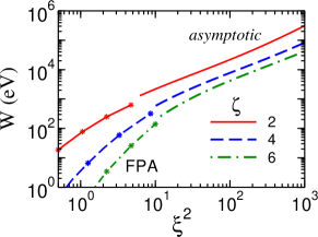
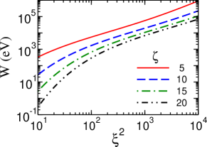
Figure 3: The total probability $W$ of the $e^{+}e^{-}$ pair production as a function of $\xi^{2}$ for various values of $\zeta$. Left panel: Results of full numerical calculation in FPA for finite values of $\xi^{2}\leq 10$ (curves marked by ”stars” in ”FPA” sections) and the asymptotic probability (20) for large values of $\xi^{2}$ (sections labeled by ”asymptotic”) at $\zeta=2$, 4 and 6. Right panel: The asymptotic probability (20) for various values of $\zeta$ as indicated in the legend.

The transition region between the two regimes is in the neighborhood of $\xi^{2}\simeq 10$. In the right panel, we show the production probability at asymptotically large values of $\xi^{2}$ for $5\leq\zeta\leq 20$. The exponential factor in (20) is most important at relatively low values of $\xi^{2}\sim 10$ (large ${\zeta}/{\xi}$). At extremely large values of $\xi^{2}$ (small ${\zeta}/{\xi}$ ), the pre-exponential factor is dominant.

3 Compton scattering in short laser pulse

The Compton scattering process, symbolically $e^{-}+L\to e^{-}{}^{\prime}+\gamma^{\prime}$ is considered here as the spontaneous emission of one photon off an electron in an external e.m. field (1). Some important aspects of generalized Compton scattering were discussed elsewhere (for references see [17]). Being crossing to the Breit-Wheeler $e^{+}e^{-}$ pair production the structure of the matrix elements and cross sections (production rates) of the both processes are the the same. The principle difference between them is absent the threshold behaviour of both processes. Thus, in Breit-Wheeler $\gamma^{\prime}+\gamma\to e^{+}+e^{-}$ one has a minimum value of the energy $\omega_{\rm min}(\gamma^{\prime})$ of the probe photon $\gamma^{\prime}$ responsible for two electron mass production (at fixed ”target” photon energy $\omega(\gamma)$). The processes with subthreshold energy $\omega^{\prime}<\omega_{\rm min}$ or sub-threshold invariant variables $\zeta>1$ are determined by the multi-photon dynamics. The Compton process $e^{-}+\gamma\to e^{-}{}^{\prime}+\gamma^{\prime}$ is always above threshold at any energy of incoming photon $\gamma$. Therefore extracting multi-photon interactions in such process is an incredibly difficult problem.

In [23] we suggested to use so-called partially integrated cross sections determined at fixed and large angle of outgoing photon $\theta^{\prime}=170^{0}$

$${\tilde{\sigma}(\omega^{\prime})}=\int\limits_{\omega^{\prime}}^{\infty}d\bar{\omega}^{\prime}\frac{d\sigma(\bar{\omega}^{\prime})}{d\bar{\omega}^{\prime}}=\int\limits_{l^{\prime}}^{\infty}dl\frac{d\sigma(l)}{dl}~{},$$ (21)

where ${d\sigma(\omega)}/{\omega}$ is the Compton scattering involving $l$ photons, while the lower limit of integration $l^{\prime}(\omega_{\rm min})$ ir related to the four momentum of incoming electron $p(E,\mathbf{p})$ and laser frequency $\omega$

$$l^{\prime}=\frac{\omega^{\prime}}{\omega}\,\frac{E+|\mathbf{p}|\cos\theta^{\prime}}{E+|\mathbf{p}|-\omega^{\prime}(1-\cos\theta^{\prime})}~{}.$$ (22)

Experimentally, this can be realized by an absorptive medium which is transparent for frequencies above a certain threshold $\omega^{\prime}$. Otherwise, such a partially integrated spectrum can be synthesized from a completely measured spectrum. Admittedly, the considered range of energies with a spectral distribution uncovering many decades is experimentally challenging. Thus the ratio $\omega^{\prime}(l)/omega^{\prime}(1)$ may be considered as a threshold parameter for the partly integrated Compron scattering.

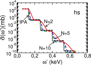
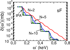
Figure 4: The partially integrated cross section (21) for $\xi^{2}=10^{-3}$. The thin solid curve marked by dots depicts the IPA result. The solid, dashed, and dot-dashed curves correspond to $N=2$, 5 and 10, respectively. Left and right panels are for hyperbolic secant (hs) and symmetrized Fermi (sF) envelopes.

The partially integrated cross sections of Eq. (21) are presented in Fig. 4. The thin solid curve (marked by dots) depicts results the photon emission in the infinite pulse (IPA) (cf. [23]). In this case the partially integrated cross section becomes a step-like function, where each new step corresponds to the contribution of a new (higher) harmonic $n$, which can be interpreted as $n$-laser photon process. Results for the finite pulse exhibited by solid, dashed, and dot-dashed curves correspond to $N=2,\,5$ and 10, respectively. In the above-threshold region with $\omega^{\prime}\leq\omega^{\prime}_{1}$, the cross sections do not depend on the widths and shapes of the envelopes, and the results of IPA and FPA coincide. The situation changes significantly in the deep sub-threshold region, where $\omega^{\prime}>\omega_{1}^{\prime}$ $(l\gg 1),\,n\gg 1$. For short pulses with $N\simeq 2$, the FPA results exceed that of IPA considerably, and the excess may reach several orders of magnitude, especially for the flat-top envelope shown by the solid curve in Fig. 4 (right panel). However, when the number of oscillation in a pulse increases ($N\gtrsim 10$) there is a qualitative convergence of FPA and IPA results, independently of the pulse shape. Thus, at $N=10$ and $\omega^{\prime}=0.6$ keV the difference between predictions for hs and sF shapes is a factor of two, as compared with the difference of the few orders of magnitude at $N=2$ for the same value of $\omega^{\prime}$.

4 Summary

In summary, we briefly discussed main aspects of multi-photon dynamics in two important OCD processes in intensive laser field: Breit-Wheeler $e^{+}e^{-}$ pair production and single photon radiation in propagation of an electron thought the laser beam. More detailed description of these and related topics may be found in our review paper [17].

References

- [1] G. A, Mourou, T Tajima, and S. V. Bulanov.// Rev. Mod. Phys. 78, 309 (2006).
- [2] A¿ Di Piazza, C. Müller, K. Z. Hatsagortsyan, and C. H. Keitel// Rev. Mod. Phys. 84, 1177 (2012).
- [3] V. Yanovsky, P. Rousseau, T. Planchon, T ,Matsuoka, A. Maksimchuk, J. Nees, G. Cheriaux, G. Mourou, K. Krushelnick.// Optics Express. 16, 2109 (2008).
-
[4]
http://www.clf.stfc.ac.uk/CLF/.
-
[5]
http://www.eli-beams.eu.
-
[6]
http://www.hiper-laser.org.
-
[7]
https://www.ipfran.ru/english/science/las_phys.html.
- [8] A. L. Cavalieri A, E. Goulielmakis, B. Horvath, W. Helml, M. Schultze, M. Fiess, V. Pervak, L. Veisz, V. S. Yakovlev, M. Uiberacker, A. Apolonski, F. Krausz, and R. Kienberger.// New J. Phys. 9, 242 (2007).
- [9] Z. Major, S. Klingebiel, C. Krobol, I. Ahmad, C. Wandt, S. A. Trushin, F. Krausz, and S. Karsch. Status of the Petawatt Field Synthesizer pump-seed synchronization measurements // AIP Conference Proceedings. 1228, 117 (2010).
- [10] F. Mackenroth, and A. Di Piazza Phys. Rev. A83, 032106 (2011).
- [11] F. Feng, S. Gilbertson, H. Mashiko, Wang He, S. D. Khan, M. Chini, Wu Yi, K. Zhao, and Z. Chang. Phys. Rev. Lett. 103, 183901 (2009).
- [12] F. Krausz, and M. Ivanov. Rev. Mod. Phys. 81, 163 2009.
- [13] H. R. Reiss. J. Math. Phys. 3, 59 (1962); Phys. Rev. Lett. 26, 1072 (1971).
- [14] A. I. Nikishov and V.‘I. Ritus. Sov. Phys. JETP. 16, 529 (1964).
- [15] N. V. Narozhny, A. I. Nikishov, and V. I. Ritus. Sov. Phys. JETP. 20, 622 (1965).
- [16] V. I. Ritus. J. Sov. Laser Res. (United States). 6:5, 497 (1985).
- [17] A. I. Titov, B. Kämpfer, A. Hosaka and H. Takabe. Phys. Part. Nucl. 47, no. 3, 456 (2016).
- [18] A. I. Titov, B. Kämpfer, H. Takabe, and A. Hosaka. Phys. Rev. Abf87, 042106 (2013).
- [19] D. M. Volkov. // Z. Phys. 94, 250 (1935).
- [20] V. B. Berestetskii, E. M. Lifshitz , and L. P. Pitaevskii. Quantum Electrodynamics. 2nd ed., (Course of theoretical physics; vol. 4.) 1982. Oxford, New York, Pergamon Press Ltd.
-
[21]
A. I. Titov, B. Kampfer, A. Hosaka, T. Nousch and D. Seipt.
Phys. Rev.D93, no. 4, 045010 (2016). - [22] G. N. Watson. A Treatise of the Theory of Bessel Functions (The University Press, Cambridge, 1944), 2nd ed.
- [23] . A. I. Titov, B. Kämpfer, T. Shibata, A. Hosaka and H. Takabe. Eur. Phys. J. D68, 299 (2014).