Highly dynamically evolved intermediate-age open clusters

Abstract

We present a comprehensive $UBVRI$ and Washington $CT_{1}T_{2}$ photometric analysis of seven catalogued open clusters, namely: Ruprecht 3, 9, 37, 74, 150, ESO 324-15 and 436-2. The multi-band photometric data sets in combination with 2MASS photometry and Gaia astrometry for the brighter stars were used to estimate their structural parameters and fundamental astrophysical properties. We found that Ruprecht 3 and ESO 436-2 do not show self-consistent evidence of being physical systems. The remained studied objects are open clusters of intermediate-age (9.0 $\leq$ log($t$ yr^-1) $\leq$ 9.6), of relatively small size ($r_{cls}$ $\sim$ 0.4 $-$ 1.3 pc) and placed between 0.6 and 2.9 kpc from the Sun. We analized the relationships between core, half-mass, tidal and Jacoby radii as well as half-mass relaxation times to conclude that the studied clusters are in an evolved dynamical stage. The total cluster masses obtained by summing those of the observed cluster stars resulted to be $\sim$ 10-15 per cent of the masses of open clusters of similar age located closer than 2 kpc from the Sun. We found that cluster stars occupy volumes as large as those for tidally filled clusters.

1 Introduction

Open clusters evolve dynamically over time due to two-body relaxation and by the external forces of the interaction with the Galactic tidal field. During this process open clusters experience structural changes (Miholics et al., 2014) which can be probed from the relationships between core, half-mass and tidal radii (Heggie & Hut, 2003), among others. In this sense, the study of highly dynamically evolved open clusters results in a challenging field of research, since they often contain few members. On the other hand, they are suited to test the particular relationships between their initial masses and dynamical ages.

Identifying dynamically evolved open clusters helps to constrain initial conditions in models which pursue describing the cluster evolution from N-body simulations (Pijloo et al., 2015; Rossi et al., 2016), such as the initial number of stars, the initial mass function, fraction of primordial binaries, etc. According to the most updated version of the open cluster catalogue compiled by Dias et al. (2002, version 3.5 as of 2016 January), a very limited number of objects have been studied with some detail from a dynamical point of view (Piskunov et al., 2007). For this reason, we have recently started to focus our long-term campaing of improving the statistics of well studied open clusters by considering their dynamical evolutions (e.g. Piatti, 2016).

In this paper, we present for the first time a comprehensive multi-band photometric analysis of seven open clusters, namely: Ruprecht 3, 9, 37, 74, 150, ESO 324-15 and 436-2 from $UBVRI$ and Washington $CT_{1}T_{2}$ photometry. Most of them turned out to be open clusters approaching their disruption stage. In Section 2 we describe the collection and reduction of the available photometric data and their thorough treatment in order to build extensive and reliable data sets. The cluster structural (e.g., core and half-light radii) and photometric (e.g., reddening, distance, age, mass) parameters are derived from star counts and colour-magnitude and colour-colour diagrams, respectively, as described in Sections 3 to 5. The analysis of the results of the different astrophysical parameters obtained is carried out in Section 6, where implications are implied. Finally, Section 7 summarizes the main conclusion of this work.

2 Data collection and reduction

We downloaded Johnson $UBV$, Kron-Cousins $RI$ and Washington $C$ images from the public website of the National Optical Astronomy Observatory (NOAO) Science Data Management (SDM) Archives. They were obtained using a 4K$\times$4K CCD detector array (scale of 0.289$\arcsec$/pixel) attached to the 1.0-m telescope at the Cerro Tololo Inter-American Observatory (CTIO), Chile, in 2011 January 31–February 4 (CTIO program #2011A-0114, PI: Clariá). Table 1 presents the log of the observations, where the main astrometric and observational information is summarized.

Table 1: Observations log of selected star clusters.

Cluster	R.A.(J2000.0)	Dec.(J2000.0)	l	b	filter	exposure	airmass	mean seeing
	(h m s)	($\degr$ $\arcmin$ $\arcsec$)	(°)	(°)		(sec)		($\arcsec$)
Ruprecht 3	6 42 6.25	-29 27 18.7	238.7690	-14.8182	$U$	90, 420	1.04, 1.03	1.2
					$B$	60, 240	1.02, 1.01	1.2
					$V$	20, 120	1.01, 1.01	1.1
					$R$	10, 90	1.00, 1.00	1.1
					$I$	10, 90	1.00, 1.00	1.1
					$C$	90, 360	1.02, 1.02	1.2
Ruprecht 9	7 2 6.94	-21 54 40.7	233.7072	-7.6073	$U$	60, 60, 480	1.03, 1.02, 1.02	1.3
					$B$	20, 60, 360	1.01, 1.01, 1.01	1.2
					$V$	20, 60, 60, 200	1.02, 1.02, 1.02, 1.01	1.2
					$R$	240, 120	1.01, 1.01	1.1
					$I$	10, 90	1.01, 1.01	1.0
					$C$	60, 400	1.01, 1.01	1.2
Ruprecht 37	7 49 46.41	-17 14 53.4	234.9286	+4.5499	$U$	90, 480	1.03, 1.03	1.2
					$B$	60, 300	1.04, 1.04	1.1
					$V$	20, 60, 180	1.05, 1.05, 1.05	1.0
					$R$	15, 120	1.06, 1.06	1.1
					$I$	10, 90	1.070, 1.070	1.1
					$C$	80, 420	1.03, 1.03	1.1
Ruprecht 74	9 21 0.55	-37 6 42.6	263.0370	+8.9625	$U$	60, 240, 540	1.01, 1.01, 1.01	1.4
					$B$	20, 200	1.03, 1.03	1.3
					$V$	15, 180	1.04, 1.04	1.1
					$R$	20, 120	1.04, 1.04	1.1
					$I$	10, 90	1.05, 1.05	1.0
					$C$	120, 480	1.02, 1.02	1.2
Ruprecht 150	7 5 55.22	-28 28 24.4	240.0141	-9.6338	$U$	60, 240	1.01, 1.02	1.2
					$B$	20, 180	1.03, 1.03	1.1
					$V$	10, 120	1.04, 1.04	1.1
					$R$	10, 90	1.05, 1.05	1.0
					$I$	10, 60	1.06, 1.06	1.1
					$C$	60, 200	1.02, 1.03	1.1
ESO 324-15	13 23 37.3	-41 53 7.5	309.3414	+20.5830	$U$	20, 200	1.04, 1.04	1.3
					$B$	10, 150	1.05, 1.05	1.1
					$V$	8, 100	1.06, 1.06	1.0
					$R$	15, 15	1.06, 1.07	1.0
					$I$	10, 80	1.08, 1.08	1.0
					$C$	20, 200	1.05, 1.05	1.3
ESO 436-02	10 14 2.76	-29 11 19.6	266.1746	+22.2431	$U$	20, 40, 180	1.01, 1.01, 1.01	1.4
					$B$	20, 150	1.02, 1.03	1.1
					$V$	4, 8, 100	1.03, 1.03, 1.03	1.0
					$R$	3, 60	1.04, 1.04	1.0
					$I$	60	1.04	1.0
					$C$	40, 180	1.02, 1.02	1.3

All the available series of bias, dome and sky flat exposures per filter during the observing nights were also downloaded to calibrate the CCD instrumental signature. We followed the data reduction procedures documented by the CTIO Y4KCam team and utilized the quadred package in IRAF. Once the calibration frames were properly combined, overscan, trimming, bias subtraction, flat corrections, etc., were performed.

In order to secure the transformation from the instrumental to the Johnson-Kron-Cousins $UBVRI$ and Washington $CT_{1}T_{2}$ standard systems, we measured nearly 150 independent magnitudes of stars per filter for each night in the standard fields SA 98 and SA 101 (Landolt, 1992; Geisler, 1996), using the apphot task within IRAF. The relationships between instrumental (i.e, measured) and standard magnitudes were obtained by fitting the equations:

$$u=u_{1}+V+(U-B)+u_{2}\times X_{U}+u_{3}\times(U-B),$$ (1)

$$b=b_{1}+V+(B-V)+b_{2}\times X_{B}+b_{3}\times(B-V),$$ (2)

$$v=v_{1}+V+v_{2}\times X_{V}+v_{3}\times(V-I),$$ (3)

$$r=r_{1}+V-(V-R)+r_{2}\times X_{R}+r_{3}\times(V-R),$$ (4)

$$i=i_{1}+V-(V-I)+i_{2}\times X_{I}+i_{3}\times(V-I),$$ (5)

$$c=c_{1}+T_{1}+(C-T_{1})+c_{2}\times X_{C}+c_{3}\times(C-T_{1}),$$ (6)

$$r={t_{1}}_{1}+T_{1}+{t_{1}}_{2}\times X_{T_{1}}+{t_{1}}_{3}\times(C-T_{1}),$$ (7)

$$t_{2}={t_{2}}_{1}+T_{1}-(T_{1}-T_{2})+{t_{2}}_{2}\times X_{T_{1}}+{t_{2}}_{3}\times(T_{1}-T_{2}),$$ (8)

where $u_{i}$, $b_{i}$, $v_{i}$, $r_{i}$, $i_{i}$, $c_{i}$, ${t_{1}}_{i}$ and ${t_{2}}_{i}$ ($i$ = 1, 2 and 3) are the fitted coefficients, and $X$ represents the effective airmass. Capital and lowercase letters represent standard and instrumental magnitudes, respectively. Here, we use $r$ magnitudes to derive $T_{1}$ magnitudes because the $R(KC)$ filter is a more efficient substitute of the Washington $T_{1}$ filter, as proposed by Geisler (1996). The transformation equations were solved with the fitparams task in IRAF for each night, and the results are shown in Table 2.

Star-finding and point-spread-function (PSF) fitting routines in the daophot/allstar suite of programs (Stetson et al., 1990) were used to derive the stellar magnitudes. For each image, a quadratically varying PSF was derived by fitting $\sim$ 200 stars, once the neighbours were eliminated using a preliminary PSF derived from the brightest, least contaminated $\sim$ 60 stars. We selected both groups of PSF stars interactively. We then used the allstar program to apply the resulting PSF to the identified stars and to create a subtracted image which was used to find and measure magnitudes of additional fainter stars. This procedure was repeated three times for each frame. After deriving the photometry for all detected stars in each filter, a cut was made on the basis of the parameters returned by DAOPHOT. Fig. 1 illustrates the typical uncertainties in the derived photometry. Only objects with $\chi$ $<$2, photometric error less than 2$\sigma$ above the mean error at a given magnitude, and $|$SHARP$|$ $<$ 0.5 were kept in each image. Aperture corrections were computed for every measured star and the mean value for each frame was used.

All individual $u,b,v,r$ and $i$ photometric files were combined into a single master file using the stand-alone daomatch and daomaster programs. We requested that at least one colour can be computed during the matching of all the photometric information for each star. Similarly, we gathered the $c,r$, and $i$ photometric files. We thus produced 2 or 3 independent $ubvri$ and $cri$ data sets, depending on the number of observations per filter available. Then we used eqs. 1–8 to standardize the resulting individual data sets, averaged the standard magnitudes and colours of each star in the different data sets, and finally cross-matched the averaged $UBVRI$ and $CT_{1}T_{2}$ data sets to build one master table per cluster field. The final information for each cluster field consists of a running number per star, its $x$ and $y$ coordinates, the mean $V$ magnitude, its rms error and the number of measurements, the colours $U-B$, $B-V$, $V-R$, $V-I$ with their respective rms errors and number of measurements, the $T_{1}$ magnitude with its error and number of measurements, and the $C-T_{1}$ and $T_{1}-T_{2}$ colours with their respective rms errors and number of measurements. Table 3 gives this information for Ruprech 3. Only a portion of this table is shown here for guidance regarding its form and content. The whole content of Table 3, as well as those for the remaining cluster fields (Tables 4-9), is available in the online version of the journal.

Figure 1: Photometric uncertainties of stars measured in the field of Ruprecht 37.

Table 2: Mean transformation coefficients for the $UBVRI$ and $CT_{1}T_{2}$ photometric systems.

Standard	zero	extinction	colour	fitting
magnitude	point	coefficient	term	rms
$U$	3.296$\pm$0.028	0.491$\pm$0.021	0.056$\pm$0.022	0.071
$B$	2.095$\pm$0.014	0.327$\pm$0.014	0.117$\pm$0.013	0.054
$V$	1.966$\pm$0.017	0.093$\pm$0.012	-0.022$\pm$0.010	0.050
$R$	1.892$\pm$0.014	0.095$\pm$0.009	-0.003$\pm$0.009	0.028
$I$	2.828$\pm$0.012	0.056$\pm$0.009	-0.022$\pm$0.004	0.031
$C$	1.904$\pm$0.021	0.514$\pm$0.017	-0.016$\pm$0.012	0.043
$T_{1}$	1.911$\pm$0.017	0.096$\pm$0.008	-0.001$\pm$0.005	0.037
$T_{2}$	2.830$\pm$0.023	0.045$\pm$0.011	0.016$\pm$0.008	0.038

Table 3: $UBVRI$ and $CT_{1}T_{2}$ data of stars in the field of Ruprecht 3.Only a portion of this table is shown here for guidance regarding its form and content.

Star	$x$	$y$	$V$	$U-B$	$B-V$	$V-R$	$V-I$	$T_{1}$	$C-T1$	$T_{1}-T_{2}$
	(pixel)	(pixel)	(mag)	(mag)	(mag)	(mag)	(mag)	(mag)	(mag)	(mag)
–	–	–	–	–	–	–	–	–	–	–
17	432.329	112.218	16.517 0.020 2	0.218 0.020 1	0.838 0.013 1	0.489 0.030 2	0.899 0.002 2	16.047 0.035 2	1.436 0.050 2	0.439 0.015 2
18	820.525	125.462	16.736 0.014 2	0.282 0.026 1	0.855 0.016 1	0.469 0.016 2	0.923 0.052 2	16.285 0.013 2	1.505 0.011 2	0.486 0.055 2
19	2486.025	126.433	16.068 0.007 2	0.119 0.021 2	0.701 0.017 2	0.446 0.037 2	0.893 0.003 2	15.641 0.015 2	1.199 0.048 2	0.479 0.020 2
–	–	–	–	–	–	–	–	–	–	–

Columns list a running number per star, its $x$ and $y$ coordinates, the mean $V$ magnitude, its rms error and the number of measurements, the colours $U-B$, $B-V$, $V-R$, $V-I$ with their respective rms errors and number of measurements, the $T_{1}$ magnitude with its error and number of measurements, and the $C-T_{1}$ and $T_{1}-T_{2}$ colours with their respective rms errors and number of measurements.

3 Cluster structural parameters

Stellar density radial profiles were built once we determined the geometrical centres of the clusters. In order to do that we fitted Gaussian distributions to the star counts in the $x$ and $y$ directions for each cluster. The fits of the Gaussians were performed using the ngaussfit routine in the stsdas/iraf package. We adopted a single Gaussian and fixed the constant to the corresponding background levels (i.e. stellar field densities assumed to be uniform) and the linear terms to zero. The centre of the Gaussian, its amplitude, and its $FWHM$ acted as variables. The number of stars projected along the $x$ and $y$ directions were counted within intervals of 20, 40, 60, 80 and 100 pixel wide, and the Gaussian fits repeated each time. Finally, we averaged the five different Gaussian centres resulting a typical standard deviation of $\pm$ 50 pixels ($\pm$ 14.5$\arcsec$) in all cases.

Subsequently stellar density profiles based on star counts previously performed within boxes of 50 pixels per side distributed throughout the whole field of each cluster were built. The chosen box size allowed us to sample the stellar spatial distribution statistically. Thus, the number of stars per unit area at a given radius $r$ can be directly calculated through the expression:

$$(n_{r+25}-n_{r-25})/(m_{r+25}-m_{r-25}),$$ (9)

where $n_{r}$ and $m_{r}$ represent the number of stars and boxes, respectively, included in a circle of radius $r$. Note that this method does not necessarily require a complete circle of radius $r$ within the observed field to estimate the mean stellar density at that distance. With a stellar density profile that extends far away from the cluster centre -but not too far so as to risk losing the local field-star signature- it is possible to estimate the background level with high precision, which is particularly useful when dealing with loose clusters. On the other hand, the more accurate the background level the more precise the cluster radius ($r_{cls}$), defined here as the distance from the cluster centre where the observed density profile intersecs the background level (see Table 10). We computed the average and corresponding rms error of the background level at any distance to the cluster centre by using every available star count measurement at that distance. Then, the mean background and its error was calculated by averaging all these latter values.

The resulting density profiles expressed as number of stars per arcsec² are shown in Fig. 2. In the figure, we represent the constructed and background subtracted density profiles with open and filled circles, respectively. Errorbars represent rms errors of star counts among boxes at the same radius, to which we added the mean error of the background star count to the background subtracted density profile. The background level and the cluster radius are indicated by solid horizontal and vertical lines, respectively; their uncertainties are in dotted lines. The normalised background corrected density profiles (those of Fig. 2) were fitted using a King (1962) model through the expression

$$N\varpropto({\frac{1}{\sqrt{1+(r/r_{c})^{2}}}-\frac{1}{\sqrt{1+(r_{t}/r_{c})^{2}}}})^{2},$$ (10)

where $r_{c}$ and $r_{t}$ are the core and tidal radii, respectively.

We also fitted Plummer (1911) profiles using the expression

$$N\varpropto\frac{1}{(1+(r/a)^{2})^{2}},$$ (11)

where $a$ is the Plummer radius, which is related to the half-mass radius ($r_{h}$) by the relation $r_{h}$ $\sim$ 1.3$a$. We used a grid of $r_{c}$ and $r_{t}$ and $r_{h}$ radii to minimize $\chi$² while fitting both King and Plummer profiles, separately. The values which best reproduce the observed stellar density profiles are listed in Table 10 and the respective King and Plummer curves are plotted with blue and orange solid lines in Fig. 2, respectively. Their uncertainties were estimated by taking into account the dispersion in the fitted density profiles.

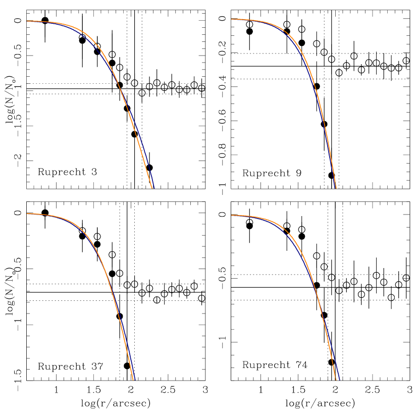
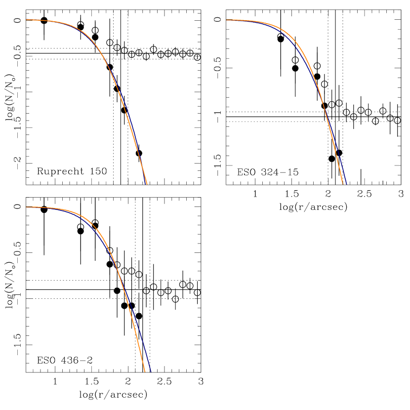
Figure 2: Stellar density profiles normalised to the central density N_o obtained from star counts. Open and filled circles refer to measured and background subtracted density profiles, respectively. The background level and the cluster radius are indicated by solid horizontal and vertical lines, respectively; their uncertainties are in dotted lines. Blue and orange solid lines depict the fitted King and Plummer curves, respectively.

4 CMD cleaning

We built six colour-magnitude diagrams (CMDs) and three colour-colour (CC) diagrams by extracting every star from our $UBVRI-CT_{1}T_{2}$ photometric data sets located within the cluster radii ($r_{cls}$). Since they account for the luminosity function, colour distribution and stellar density of the stars distributed along the cluster line of sights, we first statistically cleaned them before estimating the cluster fundamental parameters.

We performed such a cleaning of field stars by employing the procedure developed by Piatti & Bica (2012, see their Fig. 12) and also used elsewhere (e.g. Piatti, 2014; Piatti et al., 2015a; Piatti et al., 2015b; Piatti & Bastian, 2016, and references therein). The method compares a extracted cluster CMD to distinct CMDs composed of stars located reasonably far from the object, but not too far so as to risk losing the local field-star signature in terms of stellar density, luminosity function and/or colour distribution. Here we chose four field regions, each one designed to cover an equal area as that of the cluster, and placed around the cluster at $\sim$ 3-4$\times$$r_{cls}$ from the cluster centre. Note that the four selected fields could not adequately represent the fore/background of the cluster if the extinction varies significantly accross the field of view. The procedure carries out the comparison between field-star and cluster CMDs by using boxes which vary their sizes from one place to another throughout the CMD and are centred on the positions of every star found in the field-star CMD.

Since we repeated this task for each of the four field CMD box samples, we could assign a membership probability to each star in the cluster CMD. This was done by counting the number of times a star remained unsubtracted in the four cleaned cluster CMDs and by subsequently dividing this number by four. Thus, we distinguished field populations projected on to the cluster area, i.e., those stars with a probability $P$ $\leq$ 25%; stars that could equally likely be associated with either the field or the object of interest ($P$ = 50%); and stars that are predominantly found in the cleaned cluster CMDs ($P\geq$ 75%) rather than in the field-star CMDs. Statistically speaking, a certain amount of cleaning residuals is expected, which depends on the degree of variability of the stellar density, luminosity function and colour distribution of the field stars.

Figures 3 to 9 show the whole set of CMDs and CC diagrams for the cluster sample that can be exploited from the present extensive multi-band photometry. They include every magnitude and colour measurements of stars located within the respective cluster radii (see Table 10). We have also incorporated to the figures the statistical photometric memberships obtained above by distinguishing stars with different colour symbols as follows: stars that statistically belong to the field ($P\leq$ 25%, pink), stars that might belong to either the field or the cluster ($P=$ 50%, light blue), and stars that predominantly populate the cluster region ($P\geq$ 75%, dark blue). At first glance, the cleaned cluster CMDs (stars with $P\geq$ 75%) resemble those relatively poor or poor -in terms of number of stars- intermediate-age open clusters.

4.1 Proper motion

Three clusters (Ruprecht 9, 37 and 150) have been studied by Dias et al. (2014) using data from the UCAC4 (Zacharias et al., 2013) catalog in a homogeneous way. They derived mean proper motions of the clusters and the membership probabilities of the stars in the region of each cluster by applying the statistical method based on a global optimization procedure to fit the observed distribution of proper motions with two overlapping normal bivariate frequency functions, which also take the individual proper motion errors into account. We used here their membership probabilities to compare them with those coming from our photometric procedure, and to provide an independent support of identifying the fiducial CMD cluster sequences.

For the remaining clusters in the sample (Ruprecht 3, 74, ESO 324-15 and 436-2) Dias et al. (2014) could not apply their procedure, because of the small number of stars with proper motion measurements in the cluster fields. Every star with both photometric and proper motion membership probabilities $P\geq$ 75% were encircled in Figs. 3 to 9. We also searched for parallaxes and proper motions measured by the Gaia satellite (Gaia Collaboration et al., 2016) and any available information was used in Section 6.

5 Cluster fundamental parameters

The availability of six CMDs and three different CC diagrams covering wavelengths from the blue up to the near-infrared allowed us to derive reliable ages, reddenings and distances for the studied clusters. Cluster fundamental parameters were estimated following by matching theoretical isochrones to the various CMDs and CC diagrams, simultaneosly.

We used the theoretical isochrones of Bressan et al. (2012) for [Fe/H] from -0.7 to +0.2 dex, in steps of $\Delta$[Fe/H] = 0.1 dex. The adopted metallicity range covers most of that for the well-studied Milky Way open clusters (see, e.g. Paunzen et al., 2010; Heiter et al., 2014). For each [Fe/H] value we made use of the shape of the main sequence (MS), its curvatures (those less and more pronounced), the relative distance between the giant stars and the main sequence turnoff (MSTO) in magnitude and colour separately, among others, to find the age of the isochrone which best matches the cluster’s features in the CMDs and CC diagrams, regardless the cluster reddening and distance. From our best choice (this includes both [Fe/H] and age values), we derived the cluster reddenings by shifting that isochrone in the three CC diagrams following the reddening vectors until their bluest points coincided with the observed ones. Note that this requirement allowed us to use the $V-R$ vs $R-I$ CC diagram as well, even though the reddening vector runs almost parallell to the cluster sequence. Finally, the mean $E(B-V)$ colour excesses were used to properly shift the chosen isochrone in the CMDs in order to derive the cluster true distance moduli $(m-M)_{o}$ by shifting the isochrone along the magnitude axes.

In order to enter the isochrones into the CMDs and CC diagrams we used the following ratios: $E(U-B)$/$E(B-V)$ = 0.72 + 0.05$\times$$E(B-V)$ (Hiltner & Johnson, 1956); $E(V-R)$/$E(B-V)$ = 0.65, $E(V-I)$/$E(B-V)$ = 1.25, $A_{V}$/$E(B-V)$ = 3.1 (Cardelli et al., 1989); $E(C-T_{1})$/$E(B-V)$ = 1.97, $E(T_{1}-T_{2})$/$E(B-V)$ = 0.692, $A_{T_{1}}$/$E(B-V)$ = 2.62 (Geisler, 1996).

We found that isochrones bracketing the age choiced by $\Delta$ log($t$ yr^-1) = $\pm$0.10 and $\Delta$[Fe/H] = $\pm$0.10 dex represent the overall age/metallicity uncertainties owing to the observed dispersion in the cluster CMDs and CC diagrams. Fig. 4 shows the adopted isochrone (solid line) and two additional ones (dashed and dotted lines) to illustrate the overall uncertainties. The adopted best matched isochrones are overplotted on Figs. 3 to 9 with black solid lines, while the resulting values with their errors for the cluster reddenings, distances, ages and metallicities are listed in Table 10.

We additionally applied a global optimization fitting method, the Cross-Entropy (CE) technique (Monteiro et al., 2017), to estimate the fundamental parameters of the studied clusters. This is a completely independent and self-consistent procedure for analizying clusters $UBVRI$ data sets. As for the CE parameter tuning, we followed the prescriptions outlined in Monteiro et al. (2017), except the binary fraction considered here was 50$\%$ (Hurley et al., 2007; Li et al., 2012). We used the central coordinates and radii obtained in Section 3 and the stars with $P\geq$ 75% (see Section 4). Because of the small number of stars in the CMDs we did not perform neither the variation of the IMF nor the bootstrap technique. Finally, we considered the photometric errors. We found cluster parameters (reddening, distance, age and metallicity) in agreement with those derived above within the quoted uncertainties.

6 results and discussion

Ruprecht 3 has been studied by Pavani et al. (2003) from 2MASS data (Skrutskie et al., 2006). They estimated an age of log($t$ yr^-1) = 9.20$\pm$0.15, a distance from the Sun of 0.72$\pm$0.04 kpc and a colour excess $E(B-V)$= 0.04 from isochrone fitting assuming solar metal content. They suggested that the properties of Ruprecht 3 are compatible with what would be expected for an intermediate-age open cluster remnant, and described the object like a poorly populated compact concentration. Here we have made use of parallaxes ($\pi$) and proper motions ($\mu$) measured by the Gaia satellite (Gaia Collaboration et al., 2016) for five bright stars in the cluster field. They have been identified in Fig. 3 with the numbers #1 to 5 and their $\pi$ (mas), $\mu$_RA (mas/yr), $\mu$_DEC (mas/yr) values are (1.02$\pm$0.48, 1.775$\pm$1.680, -0.398$\pm$1.729)₁, (1.02$\pm$0.35, -1.027$\pm$1.747, -7.641$\pm$1.494)₂, (1.64$\pm$0.25, -0.129$\pm$1.234, 5.415$\pm$1.071)₃, (0.81$\pm$0.46, -6.115$\pm$2.593, 5.366$\pm$0.996)₄ and (3.71$\pm$0.31, -13.987$\pm$1.541, 3.563$\pm$1.312), respectively. As can be seen, ($\pi$, $\mu$_RA, $\mu$_DEC) differ among the stars, a result that agrees with the different photometric memberships of them, in the sense that values from Gaia are not expected to be identical across a sample including both members and non-members. From $\pi$ values we found that the five bright stars are located between 270 up to 1230 pc from the Sun, while their proper motions differ significantly compared to the known dispersion in stellar aggregates (Dias et al., 2014). From these values, we conclude that Ruprecht 3 is not an open cluster remnant.

Bonatto & Bica (2010) also took advantange of 2MASS data to derive an age of 3$\pm$1 Gyr, a distance from the Sun of 5.25$\pm$0.74 kpc and a colour excess $E(B-V)$ = 0.00$\pm$0.06 mag for Ruprecht 37. The cluster age agrees pretty well with our value. However, its distance differs significantly. The authors assumed [Fe/H] = 0.0 dex which is quite different to our estimated value [Fe/H] = -0.5 dex, based on the metallicity sensitive $C-T_{1}$ and $U-B$ colours. The different metallicity could affect the estimation of the remaining fundamental parameters, as well as, the fact that the 2MASS photometry is much shallower than the present one. The former barely reaches the cluster MSTO, which our photometric data sets go down $\sim$ 3 mag below the MSTO. The left-hand panel of Fig 10 shows the 2MASS CMD for stars located within the cluster radius. We have represented with blue filled circles stars that have photometric and proper motions merbership probabilitiess (see Sect. 4) higher than 75 and 70 per cent, respectively. As can be seen, the 2MASS data show a important scatter compared to the $J-H$ colour range, which makes it less reliable even when using bona-fide cluster stars.

ESO 324-15 was classified by Pavani et al. (2011) as a probable physical system, and estimated for it an age of log($t$ yr^-1) = 9.02$\pm$0.12, a colour excess $E(B-V)$ = 0.13$\pm$0.07 mag and a distance from the Sun of 0.94$\pm$0.15 kpc. They adopted [Fe/H] = 0.0 dex. Every fundamental parameter is in fairly good agreement with those derived here, except the cluster distance. The impact of such a difference can be assessed in the right-hand panel of Fig 10 where we have overplotted their selected isochrone with a solid red line.

ESO 436-02 seems to be made up of the brightest stars in the observed CMDs and CC diagrams. During the isochrone fitting, we considered as MSTO stars those at $V$ $\sim$ 10 mag (see Fig. 9). As for the CE solutions, the cluster parameters do not show Gaussian distributions as typically happens when dealing with star clusters, and the final results are not satisfactory for both the blue $B-V$ and red $V-I$ colours (see Fig 9). If we considered MSTO stars those with $V$ $<$ 12 mag, neither the isochrone fitting nor the CE method would support such an hypothesis. The Gaia parallaxes and proper motions for four bright stars, numbered #1 to 4 in Fig 9 are ($\pi$ (mas), $\mu$_RA (mas/yr), $\mu$_DEC (mas/yr) = (2.23$\pm$0.32, -3.509$\pm$0.630, -7.741$\pm$0.392))₁, (3.24$\pm$0.28, -0.400$\pm$0.674, -2.707$\pm$0.434)₂, (3.90$\pm$0.87, -19.779$\pm$2.699, 7.093$\pm$1.018)₃ and (3.75$\pm$0.26, -42.952$\pm$0.676, -11.185$\pm$0.402), respectively. From these values we conclude that the considered stars do not form a physical system.

Table 10: Derived properties of selected open clusters.

Star cluster	$E(B-V)$	$(m-M)_{o}$	d	$r_{c}$	$r_{h}$	$r_{cls}$	$r_{t}$	$\log(t)$	[Fe/H]	$t_{r}$
	(mag)	(mag)	(kpc)	(pc)	(pc)	(pc)	(pc)		(dex)	(Myr)
Ruprecht 3	0.25$\pm$0.05	10.0$\pm$0.1	1.00${}^{+0.04}_{-0.05}$	0.14$\pm$0.02	0.31$\pm$0.03	0.52${}^{+0.02}_{-0.03}$	1.70$\pm$0.24	9.0	0.0	$--$
Ruprecht 9	0.05$\pm$0.02	12.0$\pm$0.1	2.51${}^{+0.10}_{-0.11}$	0.61$\pm$0.06	1.11$\pm$0.08	1.10${}^{+0.06}_{-0.07}$	3.04$\pm$0.61	9.4	0.0	5.67$\pm$1.06
Ruprecht 37	0.20$\pm$0.04	12.3$\pm$0.1	2.88${}^{+0.13}_{-0.14}$	0.49$\pm$0.07	0.91$\pm$0.09	1.26${}^{+0.08}_{-0.09}$	3.50$\pm$0.70	9.6	-0.5	4.10$\pm$0.92
Ruprecht 74	0.00$\pm$0.03	11.3$\pm$0.1	1.82${}^{+0.09}_{-0.11}$	0.31$\pm$0.04	0.63$\pm$0.06	0.90${}^{+0.05}_{-0.06}$	3.53$\pm$0.44	9.3	0.0	2.49$\pm$0.54
Ruprecht 150	0.10$\pm$0.05	10.5$\pm$0.1	1.26${}^{+0.05}_{-0.06}$	0.21$\pm$0.03	0.40$\pm$0.04	0.48${}^{+0.03}_{-0.04}$	1.53$\pm$0.30	9.2	0.0	1.00$\pm$0.29
ESO 324-15	0.15$\pm$0.04	9.0$\pm$0.1	0.63${}^{+0.01}_{-0.03}$	0.12$\pm$0.01	0.26$\pm$0.02	0.38${}^{+0.02}_{-0.03}$	1.38$\pm$0.15	9.1	0.0	0.67$\pm$0.13
ESO 436-2	0.00$\pm$0.05	8.9$\pm$0.1	0.60${}^{+0.01}_{-0.02}$	0.12$\pm$0.01	0.25$\pm$0.02	0.46${}^{+0.01}_{-0.02}$	1.61$\pm$0.15	9.1	-0.2	$--$

Note: to convert 1 arcsec to pc, we use the following expression,10$\times$10${}^{(m-M)_{o}/5}$sin(1/3600) where $(m-M)_{o}$ is the true distance modulus.

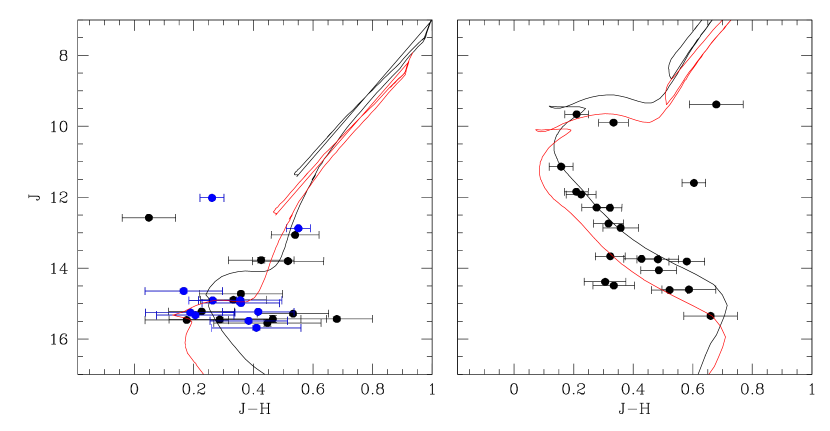
Figure 10: 2MASS CMDs for stars located within the cluster radius of Ruprecht 37 (left-hand panel), and ESO 324-15 (right-hand panel). Blue filled circles (and respective errorbars) represent stars with photometric and proper motion membership probabilities higher than 75 and 70 per cent, respectively. Theoretical isochrones of Bressan et al. (2012) for the cluster fundamental parameters estimated previously and in this work are superimposed with solid red and black lines, respectively (see Sect. 6 for details).

Table 11: Derived masses (M_⊙) of selected open clusters.

Star cluster	$M_{total}$	$M_{J16}$	$M_{Salpeter}$
Ruprecht 9	10.3$\pm$4.7	82$\pm$88	130
Ruprecht 37	46.3$\pm$21.3	70$\pm$77	125
Ruprecht 74	13.8$\pm$6.3	90$\pm$96	150
Ruprecht 150	13.5$\pm$6.2	97$\pm$101	170
ESO 324-15	14.1$\pm$6.4	106$\pm$111	135

We derived the masses of Ruprecht 9, 37, 74, 150 and ESO 324-15 by summing the individual masses of stars with membership probabilities $P\geq$ 75%. The latter were obtained by interpolation in the theoretical isochrones traced in Figs. 4 to 8 from the observed $V$ magnitude of each star, properly corrected by reddening and distance modulus. We estimate the uncertainty in the mass to be $\sigma(\log(M/\hbox{M${}_{\odot}$}))$ $\sim$ 0.2 dex. Note that this error comes from propagation of the $V$ magnitude errors in the mass distribution along the theoretical isochrones. It does not reflect the deviation of the cluster mass computed from stars with $P\geq$ 75% from the actual cluster mass. Nevertheless, at first glance, the appearance of the cluster CMDs and CC diagrams ($P\geq$ 75%) do not seem to significantly differ from those including any other observed stars placed along the adopted isochrones with $P<$ 75%, thought to be cluster stars. The derived total cluster masses ($M_{total}$) of Ruprecht 9, 37, 74, 150 and ESO 324-15 are listed in Table 11. The resulting cluster mass functions (MFs) are shown in Fig. 11 where the errorbars come from applying Poisson statistics. The solid lines represent the relationship given by Salpeter (1955, slope = -2.35) for the stars in the solar neighbourhood.

We also used the relationship between the cluster mass and the cluster age derived by Joshi et al. (2016, their equation 8) from 489 open clusters located closer than 2 kpc from the Sun, to estimate the masses of the clusters in our sample. The computed masses ($M_{J16}$) are listed in Table 11. As can be seen, the $M_{total}$ values resulted to be $\sim$ 10-15 per cent of $M_{J16}$ ones, except for Ruprecht 37 whose $M_{total}$ is $\sim$ 65 per cent of its $M_{J16}$ value. Alternatively, in order to have some other rough estimate of upper mass limits, we used the Salpeter’s law along with the zero points in Fig. 11, to estimate the cluster mass ($M_{Salpeter}$) down to a star mass of 0.5M_⊙. We derived masses 35-40 per cent larger than $M_{J16}$, except for ESO 324-15 whose $M_{Salpeter}$ value resulted to be 20 per cent larger that those from Joshi et al. (2016), respectively (see Table 11).

Using the half-mass radii $r_{h}$ and masses of Table 11, we computed the half-mass relaxation times using the equation (Spitzer & Hart, 1971):

$$t_{r}=\frac{8.9\times 10^{5}M_{cls}^{1/2}r_{h}^{3/2}}{\bar{m}log_{10}(0.4M_{cls}/\bar{m})},$$ (12)

where $M_{cls}$ is the $M_{J16}$ value and $\bar{m}$ is the mean mass of the cluster stars. We used $\sigma$$M_{J16}$ and $\sigma$$r_{h}$ to estimate $\sigma$$t_{h}$. The resulting $t_{r}$ values are listed in the last column of Table 10.

Figure 11: Mass function for clusters in our sample. The solid lines represent the relationship given by Salpeter (1955, slope = -2.35) for the stars in the solar neighbourhood.

The comparison of the cluster ages with their respective $t_{r}$ values clearly reveals that all the clusters in the sample have survived hundreds of times their characteristic two-body relaxation times and should be much closer to a disruption stage. Their total masses, which represent a mass loss around 85-90 per cent from their $M_{J16}$ values -with the sole exception of Ruprecht 37 whose mass loss is around 35 per cent-, also confirm such a highly evolved dynamical stage. If we considered the $M_{Salpeter}$ values as the initial cluster masses instead, the mass loss would be still larger. Note that the mass loss is due to both internal dynamical evolution and tidal effects. As for the Galactic tidal field, Miholics et al. (2014, see, e.g., their figures 1) found that the difference in the potential wall between 6 and 100 kpc from the galactic centre leads to $\leq$ 10 per cent variations in the half-mass radius for clusters younger than 4 Gyr. Thus, bearing in mind the Galactocentric distances of the studied clusters ($R_{GC}$ = 9 $\pm$ 1 kpc) and their ages (see Table 10), we considered the dynamical evolution as the main origin of mass loss. The effect of an important mass loss stand out in Fig 11 where the observed MFs depart from that of the Salpeter’s law towards lower stellar masses. Surprinsingly enough is the fact that even though the surviving clusters keep small amounts of their $M_{J16}$ and $M_{Salpeter}$ masses, the cluster CMDs are still useful to derive their fundamental paramaters.

From the analysis of the derived structural paramaters, it is also feasible to draw conclusions about their present dynamical stage. Trenti et al. (2010) presented a unified picture for the evolution of star clusters on the two-body relaxation timescale from direct N-body simulations of star clusters in a tidal field. Their treatment of the stellar evolution is based on the approximation that most of the relevant stellar evolution occurs on a timescale shorter than a relaxation time, when the most massive stars lose a significant fraction of mass and consequently contribute to a global expansion of the system. Later in the life of a star cluster, two-body relaxation tends to erase the memory of the initial density profile and concentration. They found that the structure of the system, as measured by the core to half-mass radius ratio, the concentration parameter $c$= log($r_{t}/r_{c}$), among others, evolve toward a universal state, which is set by the efficiency of heating on the visible population of stars induced by dynamical interactions in the core of the system. The concentration parameter $c$ for this model increases steadily with time.

The resulting $c$ values for our clusters are within 0.9 and 1.1 (0.7 for Ruprecht 9). These values correspond to star clusters in an advance stage of dynamical evolution. Indeed, we compared our $c$ values with those for 236 open clusters analyzed by Piskunov et al. (2007), who derived from them homogeneous scales of radii and masses. They derived core and tidal radii for their cluster sample, from which we calculated the half-mass radii and, with their clusters masses and equation 10, relaxation times, by assuming that the cluster stellar density profiles can be indistinguishably reproduced by King and Plummer models. Their cluster sample is mostly distributed inside a circle of $\sim$ 1 kpc from the Sun and has $c$ values between $\sim$ 0.1 up to 1.1 following a broad trend with the age/$t_{r}$ ratio, in the sense that the larger the $c$ values, the more dynamically evolved an open cluster.

According to Heggie & Hut (2003, see, e.g., their figure 33.2) a star cluster dynamically evolving with its tidal radius filled, moves in the $r_{c}/r_{h}$ vs $r_{h}/r_{t}$ plane parallel to the $r_{c}/r_{h}$ axis ($r_{h}/r_{t}$ $\sim$ 0.21) toward low values due to violent relaxation in the cluster core region followed by two-body relaxation, mass segregation, and finally core-collapse. The derived $r_{h}/r_{t}$ ratio for the present cluster sample is 0.22 $\pm$ 0.07 (see Table 10), which is in excellent agreement with the expected value for a tidally filled cluster. Curiously, the tidal radii are quit similar to the Jacobi radii, which confirm that the studied clusters are tidally filled. The latter were calculated using the expresion (Chernoff & Weinberg, 1990) :

$$r_{J}=(\frac{M_{cls}}{3M_{gal}})^{1/3}\times R_{GC},$$ (13)

where $M_{cls}$ is the cluster mass and $M_{gal}$ is the Milky Way (MW) mass inside the cluster galactocentric distance $R_{GC}$. To compute $M_{gal}$ (= 5$\times$10¹¹M_⊙) we used the MW mass profile of Taylor et al. (2016). We found that $|$$r_{t}$-$r_{J}$$|$ $<$ $\sigma$$r_{t}$ + $\sigma$$r_{J}$, meaning that cluster stars have occupied as much as possible the allowed volume without being stripped away from the cluster. In the same model by Heggie & Hut (2003), the $r_{c}/r_{h}$ ratio ranges from 1.4 (start of evolution) down to 0.1. The $r_{c}/r_{h}$ ratio of the studied clusters is 0.49 $\pm$ 0.06, which confirms their evolved dynamical stages.

7 conclusions

We present a comprehensive multi-band photometric analysis of seven catalogued open clusters, namely: Ruprecht 3, 9, 37, 74, 150, ESO 324-15 and 436-2. The objects were observed through the Johnson $UBV$, Kron-Cousins $RI$ and Washington $C$ filters; four of them (Ruprecht 9, 74, 150 and ESO 436-2) are photometrically study for the first time, while for Ruprecht 3, 37 and ESO 324-15, our photometric data sets surpass that from 2MASS photometry.

The multi-band photometric data sets were used to trace the cluster stellar density radial profiles and to build CMDs and CC diagrams, from which we estimated their structural parameters and fundamental astrophysical properties. Cluster radii were derived from a careful placement of the background levels in the radial profiles built from star count throughout the observed fields using the final photometric catalogues. We fitted King and Plummer models to derive cluster core, half-mass and tidal radii.

The constructed cluster CMDs and CC diagrams were statistically cleaned from field star contamination using a powerful technique that makes use of cells varying in position and size in order to reproduce the field CMD as closely as possible. Then, from six cleaned CMDs and three cleaned CC diagrams covering wavelengths from the blue up to the near-infrared we estimated the cluster fundamental parameters. We exploited such a wealth in combination with theoretical isochrones to find out that the clusters in our sample are of intermediate-age (9.0 $\leq$ log($t$ yr^-1) $\leq$ 9.6), of relatively small size ($r_{cls}$ $\sim$ 0.4 $-$ 1.3 pc) and placed between 0.6 and 2.9 kpc from the Sun. Their total masses, computed by summing the individual masses of stars with photometric membership probabilities $P\geq$ 75%, resulted to be $\sim$ 10-15 per cent of the cluster masses estimated from an independent robust calibration of the cluster mass as a function of the cluster age. The cluster MFs built using the same sample of stars also account for so high percentage of mass loss. We found that Ruprecht 3 and ESO 436-2 do not show self-consistent evidence to be physical systems.

We compared the cluster masses, concentration parameters, $r_{c}/r_{h}$, $r_{h}/r_{t}$ and age/$t_{r}$ ratios to those for 236 clusters located in the solar neighbourhood as well as to different theoretical models. We conclude that the studied clusters should be much closer to their disruption stage as a result of their internal dynamical evolution (mass segregation) and Galactic tidal effects. The stars with photometric membership probabilities $P\geq$ 75% occupy a volume as large as those for tidally filled clusters.

Figure 3: CMDs and CC diagrams for stars measured in the field of Rupreht 3. Colour-scaled symbols represent stars with photometric memberships $P\leq$ 25% (pink), equals to 50% (light blue) and $\geq$ 75% (dark blue), respectively. We overplotted the isochrones which best matches the cluster features (black solid line). Stars with Gaia parallaxes and proper motions are numbered from #1 to 5 (see text for details).

Figure 4: CMDs and CC diagrams for stars measured in the field of Ruprecht 9. Symbols are as in Fig. 3. Dashed and dotted lines correspond to isochrones for (log($t$ yr^-1), [Fe/H]) = (9.3,-0.1) and (9.5,+0.1), respectively. Large open circles represent stars with both photometric ($P\geq$ 75%) and proper motion ($P\geq$ 75%) membership probabilities (see text for details).

Figure 5: CMDs and CC diagrams for stars measured in the field of Ruprecht 37. Symbols are as in Fig. 3. Large open circles represent stars with both photometric ($P\geq$ 75%) and proper motion ($P\geq$ 75%) membership probabilities (see text for details).

Figure 6: CMDs and CC diagrams for stars measured in the field of Ruprecht 74. Symbols are as in Fig. 3.

Figure 7: CMDs and CC diagrams for stars measured in the field of Ruprecht 150. Symbols are as in Fig. 3. Large open circles represent stars with both photometric ($P\geq$ 75%) and proper motion ($P\geq$ 75%) membership probabilities (see text for details).

Figure 8: CMDs and CC diagrams for stars measured in the field of ESO 324-15. Symbols are as in Fig. 3.

Figure 9: CMDs and CC diagrams for stars measured in the field of ESO 436-2. Symbols are as in Fig. 3. Stars with Gaia parallaxes and proper motions are numbered from #1 to 4. (see text for details).

References

- Bonatto & Bica (2010) Bonatto C., Bica E., 2010, MNRAS, 407, 1728
- Bressan et al. (2012) Bressan A., Marigo P., Girardi L., Salasnich B., Dal Cero C., Rubele S., Nanni A., 2012, MNRAS, 427, 127
- Cardelli et al. (1989) Cardelli J. A., Clayton G. C., Mathis J. S., 1989, ApJ, 345, 245
- Chernoff & Weinberg (1990) Chernoff D. F., Weinberg M. D., 1990, ApJ, 351, 121
- Dias et al. (2002) Dias W. S., Alessi B. S., Moitinho A., Lépine J. R. D., 2002, A&A, 389, 871
- Dias et al. (2014) Dias W. S., Monteiro H., Caetano T. C., Lépine J. R. D., Assafin M., Oliveira A. F., 2014, A&A, 564, A79
- Gaia Collaboration et al. (2016) Gaia Collaboration Brown A. G. A., Vallenari A., Prusti T., de Bruijne J., Mignard F., Drimmel R., co-authors ., 2016, preprint, (arXiv:1609.04172)
- Geisler (1996) Geisler D., 1996, AJ, 111, 480
- Heggie & Hut (2003) Heggie D., Hut P., 2003, The Gravitational Million-Body Problem: A Multidisciplinary Approach to Star Cluster Dynamics
- Heiter et al. (2014) Heiter U., Soubiran C., Netopil M., Paunzen E., 2014, A&A, 561, A93
- Hiltner & Johnson (1956) Hiltner W. A., Johnson H. L., 1956, ApJ, 124, 367
- Hurley et al. (2007) Hurley J. R., Aarseth S. J., Shara M. M., 2007, ApJ, 665, 707
- Joshi et al. (2016) Joshi Y. C., Dambis A., Pandey A. K., Joshi S., 2016, preprint, (arXiv:1606.06425)
- King (1962) King I., 1962, AJ, 67, 471
- Landolt (1992) Landolt A. U., 1992, AJ, 104, 340
- Li et al. (2012) Li Z., Mao C., Chen L., Zhang Q., 2012, ApJ, 761, L22
- Miholics et al. (2014) Miholics M., Webb J. J., Sills A., 2014, MNRAS, 445, 2872
- Monteiro et al. (2017) Monteiro H., Dias W. S., Hickel G. R., Caetano T. C., 2017, New Astron., 51, 15
- Paunzen et al. (2010) Paunzen E., Heiter U., Netopil M., Soubiran C., 2010, A&A, 517, A32
- Pavani et al. (2003) Pavani D. B., Bica E., Ahumada A. V., Clariá J. J., 2003, A&A, 399, 113
- Pavani et al. (2011) Pavani D. B., Kerber L. O., Bica E., Maciel W. J., 2011, MNRAS, 412, 1611
- Piatti (2014) Piatti A. E., 2014, MNRAS, 440, 3091
- Piatti (2016) Piatti A. E., 2016, MNRAS,
- Piatti & Bastian (2016) Piatti A. E., Bastian N., 2016, preprint, (arXiv:1603.06891)
- Piatti & Bica (2012) Piatti A. E., Bica E., 2012, MNRAS, 425, 3085
- Piatti et al. (2015a) Piatti A. E., de Grijs R., Rubele S., Cioni M.-R. L., Ripepi V., Kerber L., 2015a, MNRAS, 450, 552
- Piatti et al. (2015b) Piatti A. E., et al., 2015b, MNRAS, 454, 839
- Pijloo et al. (2015) Pijloo J. T., Portegies Zwart S. F., Alexander P. E. R., Gieles M., Larsen S. S., Groot P. J., Devecchi B., 2015, MNRAS, 453, 605
- Piskunov et al. (2007) Piskunov A. E., Schilbach E., Kharchenko N. V., Röser S., Scholz R.-D., 2007, A&A, 468, 151
- Plummer (1911) Plummer H. C., 1911, MNRAS, 71, 460
- Rossi et al. (2016) Rossi L. J., Bekki K., Hurley J. R., 2016, MNRAS, 462, 2861
- Salpeter (1955) Salpeter E. E., 1955, ApJ, 121, 161
- Skrutskie et al. (2006) Skrutskie M. F., et al., 2006, AJ, 131, 1163
- Spitzer & Hart (1971) Spitzer Jr. L., Hart M. H., 1971, ApJ, 164, 399
- Stetson et al. (1990) Stetson P. B., Davis L. E., Crabtree D. R., 1990, in Jacoby G. H., ed., Astronomical Society of the Pacific Conference Series Vol. 8, CCDs in astronomy. pp 289–304
- Taylor et al. (2016) Taylor C., Boylan-Kolchin M., Torrey P., Vogelsberger M., Hernquist L., 2016, MNRAS, 461, 3483
- Trenti et al. (2010) Trenti M., Vesperini E., Pasquato M., 2010, ApJ, 708, 1598
- Zacharias et al. (2013) Zacharias N., Finch C. T., Girard T. M., Henden A., Bartlett J. L., Monet D. G., Zacharias M. I., 2013, AJ, 145, 44