Mismatched Multi-letter Successive
Decoding for the Multiple-Access Channel

Abstract

This paper studies channel coding for the discrete memoryless multiple-access channel with a given (possibly suboptimal) decoding rule. A multi-letter successive decoding rule depending on an arbitrary non-negative decoding metric is considered, and achievable rate regions and error exponents are derived both for the standard MAC (independent codebooks), and for the cognitive MAC (one user knows both messages) with superposition coding. In the cognitive case, the rate region and error exponent are shown to be tight with respect to the ensemble average. The rate regions are compared with those of the commonly-considered decoder that chooses the message pair maximizing the decoding metric, and numerical examples are given for which successive decoding yields a strictly higher sum rate for a given pair of input distributions.

I Introduction

The mismatched decoding problem [1, 2, 3] seeks to characterize the performance of channel coding when the decoding rule is fixed and possibly suboptimal (e.g., due to channel uncertainty or implementation constraints). Extensions of this problem to multiuser settings are not only of interest in their own right, but can also provide valuable insight into the single-user setting [3, 4, 5]. In particular, significant attention has been paid to the mismatched multiple-access channel (MAC), described as follows. User $\nu=1,2$ transmits a codeword $\boldsymbol{x}_{\nu}$ from a codebook $\mathcal{C}_{\nu}=\{\boldsymbol{x}_{\nu}^{(1)},\cdots,\boldsymbol{x}_{\nu}^{(M_{\nu})}\}$, and the output sequence $\boldsymbol{y}$ is generated according to $W^{n}(\boldsymbol{y}|\boldsymbol{x}_{1},\boldsymbol{x}_{2})\triangleq\prod_{i=1}^{n}W(y_{i}|x_{1,i},x_{2,i})$ for some transition law $W(y|x_{1},x_{2})$. The mismatched decoder estimates the message pair as

$$(\hat{\mathsf{m}}_{1},\hat{\mathsf{m}}_{2})=\arg\max_{(i,j)}q^{n}(\boldsymbol{x}_{1}^{(i)},\boldsymbol{x}_{2}^{(j)},\boldsymbol{y}),$$ (1)

where $q^{n}(\boldsymbol{x}_{1},\boldsymbol{x}_{2},\boldsymbol{y})\triangleq\prod_{i=1}^{n}q(x_{1,i},x_{2,i},y_{i})$ for some non-negative decoding metric $q(x_{1},x_{2},y)$. The metric $q(x_{1},x_{2},y)=W(y|x_{1},x_{2})$ corresponds to optimal maximum-likelihood (ML) decoding, whereas the introduction of mismatch can significantly increase the error probability and lead to smaller achievable rate regions [1, 3]. Even in the single-user case, characterizing the capacity with mismatch is a long-standing open problem.

Given that the decoder only knows the metric $q^{n}(\boldsymbol{x}_{1}^{(i)},\boldsymbol{x}_{2}^{(j)},\boldsymbol{y})$ corresponding to each codeword pair, one may question whether there exists a decoding rule that provides better performance than the maximum-metric rule in (1), and that is well-motivated from a practical perspective. The second of these requirements is not redundant; for instance, if the values $\{\log q(x_{1},x_{2},y)\}$ are rationally independent (i.e., no values can be written as linear combinations of the others with rational coefficients), then one could consider a highly artificial and impractical decoder that uses these values to infer the joint empirical distribution of $(\boldsymbol{x}_{1},\boldsymbol{x}_{2},\boldsymbol{y})$, and in turn uses that to implement the maximum-likelihood (ML) rule. While such a decoder is a function of $\{q^{n}(\boldsymbol{x}_{1}^{(i)},\boldsymbol{x}_{2}^{(j)},\boldsymbol{y})\}_{i,j}$ and clearly outperforms the maximum-metric rule, it does not bear any practical interest.

There are a variety of well-motivated decoding rules that are of interest beyond maximum-metric, including threshold decoding [6, 7], likelihood decoding [8, 9], and successive decoding [10, 11]. In this paper, we focus on the latter, and consider the following two-step decoding rule:

$$\hat{\mathsf{m}}_{1} =\arg\max_{i}\sum_{j}q^{n}(\boldsymbol{x}_{1}^{(i)},\boldsymbol{x}_{2}^{(j)},\boldsymbol{y}),$$ (2)

$$\hat{\mathsf{m}}_{2} =\arg\max_{j}q^{n}(\boldsymbol{x}_{1}^{(\hat{\mathsf{m}}_{1})},\boldsymbol{x}_{2}^{(j)},\boldsymbol{y}).$$ (3)

The study of this decoder is of interest for several reasons:

• The decoder depends on the exact same quantities as the maximum-metric decoder (1) (namely, $q^{n}(\boldsymbol{x}_{1}^{(i)},\boldsymbol{x}_{2}^{(j)},\boldsymbol{y})$ for each $(i,j)$), meaning a comparison of the two rules is in a sense fair. We will see the successive rule can sometimes achieve rates that are not achieved by the maximum-metric rule (in the random coding regime), which is the first result of this kind for the mismatched MAC.

• The first decoding step (2) can be considered a mismatched version of the optimal decoding rule for (one user of) the interference channel. Hence, as well as giving an achievable rate region for the MAC with mismatched successive decoding, our results directly quantify the loss due to mismatch for the interference channel.

• More broadly, successive decoding is of significant practical interest for multiple-access scenarios, since it permits the use of single-user codes, as well as linear decoding complexity in the number of users [11]. While the specific successive decoder that we consider does not enjoy these practical benefits, it may still serve as an interesting point of comparison for such variants.

The rule in (2) is multi-letter, in the sense that the objective function does not factorize into a product of $n$ symbols on $(\mathcal{X}_{1},\mathcal{Y})$. Single-letter successive decoders [10, Sec. 4.5.1] could also potentially be studied from a mismatched decoding perspective by introducing a second decoding metric $q_{2}(x_{1},y)$, but we focus on the above rule depending only on a single metric $q(x_{1},x_{2},y)$.

Under the above definitions of $W$, $q$, $W^{n}$ and $q^{n}$, and assuming the corresponding alphabets $\mathcal{X}_{1}$, $\mathcal{X}_{2}$ and $\mathcal{Y}$ to be finite, we consider two distinct classes of MACs:

1. For the standard MAC [3], encoder $\nu=1,2$ takes as input $\mathsf{m}_{\nu}$ equiprobable on $\{1,\cdots,M_{\nu}\}$, and transmits the corresponding codeword $\boldsymbol{x}_{\nu}^{(\mathsf{m}_{\nu})}$ from a codebook $\mathcal{C}_{\nu}$.

2. For the cognitive MAC [4] (or MAC with degraded message sets [10, Ex. 5.18]), the messages $\mathsf{m}_{\nu}$ are still equiprobable on $\{1,\cdots,M_{\nu}\}$, but user 2 has access to both messages, while user 1 only knows $\mathsf{m}_{1}$. Thus, $\mathcal{C}_{1}$ contains codewords indexed as $\boldsymbol{x}_{1}^{(i)}$, and $\mathcal{C}_{2}$ contains codewords indexed as $\boldsymbol{x}_{2}^{(i,j)}$.

For each of these, we say that a rate pair $(R_{1},R_{2})$ is achievable if, for all $\delta>0$, there exist sequences of codebooks $\mathcal{C}_{1,n}$ and $\mathcal{C}_{2,n}$ with $M_{1}\geq e^{n(R_{1}-\delta)}$ and $M_{2}\geq e^{n(R_{2}-\delta)}$ respectively, such that the error probability

$$p_{\mathrm{e}}\triangleq\mathbb{P}[(\hat{\mathsf{m}}_{1},\hat{\mathsf{m}}_{2})\neq(\mathsf{m}_{1},\mathsf{m}_{2})]$$ (4)

tends to zero under the decoding rule described by (2)–(3). Our results will not depend on the method for breaking ties, so for concreteness, we assume that ties are broken as errors.

For fixed rates $R_{1}$ and $R_{2}$, an error exponent $E(R_{1},R_{2})$ is said to be achievable if there exists a sequence of codebooks $\mathcal{C}_{1,n}$ and $\mathcal{C}_{2,n}$ with $M_{1}\geq\exp(nR_{1})$ and $M_{2}\geq\exp(nR_{2})$ codewords of length $n$ such that

$$\liminf_{n\to\infty}-\frac{1}{n}\log p_{\mathrm{e}}\geq E(R_{1},R_{2}).$$ (5)

Letting $\mathcal{E}_{\nu}\triangleq\{\hat{\mathsf{m}}_{\nu}\neq\mathsf{m}_{\nu}\}$ for $\nu=1,2$, we observe that if $q(x_{1},x_{2},y)=W(y|x_{1},x_{2})$, then (2) is the decision rule that minimizes $\mathbb{P}[\mathcal{E}_{1}]$. Using this observation, we show in Appendix A that the successive decoder with $q=W$ is guaranteed to achieve the same rate region and error exponent as that of optimal non-successive maximum-likelihood decoding.

I-A Previous Work and Contributions

The vast majority of previous works on mismatched decoding have focused on achievability results via random coding, and the only general converse results are written in terms of non-computable information-spectrum type quantities [7]. For the point-to-point setting with mismatch, the asymptotics of random codes with independent codewords are well-understood for the i.i.d. [12], constant-composition [13, 14, 1, 15] and cost-constrained [2, 16] ensembles. Dual expressions and continuous alphabets were studied in [15] and [2].

The mismatched MAC was introduced by Lapidoth [3], who showed that $(R_{1},R_{2})$ is achievable provided that

$$R_{1} \leq\min_{\begin{subarray}{c}\widetilde{P}_{X_{1}X_{2}Y}\,:\,\widetilde{P}_{X_{1}}=Q_{1},\widetilde{P}_{X_{2}Y}=P_{X_{2}Y},\\ \mathbb{E}_{\widetilde{P}}[\log q(X_{1},X_{2},Y)]\geq\mathbb{E}_{P}[\log q(X_{1},X_{2},Y)]\end{subarray}}I_{\widetilde{P}}(X_{1};X_{2},Y),$$ (6)

$$R_{2} \leq\min_{\begin{subarray}{c}\widetilde{P}_{X_{1}X_{2}Y}\,:\,\widetilde{P}_{X_{2}}=Q_{2},\widetilde{P}_{X_{1}Y}=P_{X_{1}Y},\\ \mathbb{E}_{\widetilde{P}}[\log q(X_{1},X_{2},Y)]\geq\mathbb{E}_{P}[\log q(X_{1},X_{2},Y)]\end{subarray}}I_{\widetilde{P}}(X_{2};X_{1},Y),$$ (7)

$$R_{1}+R_{2} \leq\min_{\begin{subarray}{c}\widetilde{P}_{X_{1}X_{2}Y}\,:\,\widetilde{P}_{X_{1}}=Q_{1},\widetilde{P}_{X_{2}}=Q_{2},\widetilde{P}_{Y}=P_{Y}\\ \mathbb{E}_{\widetilde{P}}[\log q(X_{1},X_{2},Y)]\geq\mathbb{E}_{P}[\log q(X_{1},X_{2},Y)]\\ I_{\widetilde{P}}(X_{1};Y)\leq R_{1},\,I_{\widetilde{P}}(X_{2};Y)\leq R_{2}\end{subarray}}D(\widetilde{P}_{X_{1}X_{2}Y}\|Q_{1}\times Q_{2}\times\widetilde{P}_{Y}),$$ (8)

where $Q_{1}$ and $Q_{2}$ are arbitrary input distributions, and $P_{X_{1}X_{2}Y}\triangleq Q_{1}\times Q_{2}\times W$. The corresponding ensemble-tight error exponent was given by the present authors in [5], along with equivalent dual expressions and generalizations to continuous alphabets. Error exponents were also presented for the MAC with general decoding rules in [17], but the results therein are primarily targeted to optimal or universal metrics; in particular, when applied to the mismatched setting, the exponents are not ensemble-tight.

The mismatched cognitive MAC was introduced by Somekh-Baruch [4], who used superposition coding to show that $(R_{1},R_{2})$ is achievable provided that

$$R_{2} \leq\min_{\begin{subarray}{c}\widetilde{P}_{X_{1}X_{2}Y}\,:\,\widetilde{P}_{X_{1}X_{2}}=Q_{X_{1}X_{2}},\widetilde{P}_{X_{1}Y}=P_{X_{1}Y},\\ \mathbb{E}_{\widetilde{P}}[\log q(X_{1},X_{2},Y)]\geq\mathbb{E}_{P}[\log q(X_{1},X_{2},Y)]\end{subarray}}I_{\widetilde{P}}(X_{2};Y|X_{1}),$$ (9)

$$R_{1}+R_{2} \leq\min_{\begin{subarray}{c}\widetilde{P}_{X_{1}X_{2}Y}\,:\,\widetilde{P}_{X_{1}X_{2}}=Q_{X_{1}X_{2}},\widetilde{P}_{Y}=P_{Y},\\ \mathbb{E}_{\widetilde{P}}[\log q(X_{1},X_{2},Y)]\geq\mathbb{E}_{P}[\log q(X_{1},X_{2},Y)],\,I_{\widetilde{P}}(X_{1},;Y)\leq R_{1}\end{subarray}}I_{\widetilde{P}}(X_{1},X_{2};Y),$$ (10)

where $Q_{X_{1}X_{2}}$ is an arbitrary input distribution, and $P_{X_{1}X_{2}Y}\triangleq Q_{X_{1}X_{2}}\times W$. The corresponding ensemble-tight error exponent was also given therein. Various forms of superposition coding were also studied by the present authors in [5], but with a focus on the single-user channel as opposed to the cognitive MAC.

Both of the above regions are known to be tight with respect to the ensemble average for constant-composition random coding, meaning that any looseness is due to the random-coding ensemble itself, rather than the bounding techniques used in the analysis [3, 4]. This notion of tightness was first explored in the single-user setting in [15]. We also note that the above regions lead to improved achievability bounds for the single-user setting [3, 4].

The main contributions of this paper are achievable rate regions for both the standard MAC (Section II-A) and cognitive MAC (Section II-B) under the successive decoding rule in (2)–(3). For the cognitive case, we also provide an ensemble tightness result. Both regions are numerically compared to their counterparts for maximum-metric decoding, and in each case, it is observed that the successive rule can provide a strictly higher sum rate, though neither the successive nor maximum-metric region is included in the other in general.

A by-product of our analysis is achievable error exponents corresponding to the rate regions. Our exponent for the standard MAC is related to that of Etkin et al. [18] for the interference channel, as both use parallel coding. Similarly, our exponent for the cognitive MAC is related to that of Kaspi and Merhav [19], since both use superposition coding. Like these works, we make use of type class enumerators; however, a key difference is that we avoid applying a Gallager-type bound in the initial step, and we instead proceed immediately with type-based methods.

In a work that developed independently of ours, the interference channel perspective was pursued in depth in the matched case in [20], with a focus on error exponents. The error exponent of [20] is similar to that derived in the present paper, but also contains an extra maximization term that, at least in principle, could improve the exponent. Currently, no examples are known where such an improvement is obtained. Moreover, while the analysis techniques of [20] extend to the mismatched case, doing so leads to the same achievable rate region as ours; the only potential improvement is in the exponent. Finally, we note that while our focus is solely on codebooks with independent codewords, error exponents were also given for the Han-Kobayashi construction in [20].

Another line of related work studied the achievable rates of polar coding with mismatch [21, 22, 23, 24], using a computationally efficient successive decoding rule. A single-letter achievable rate was given, and it was shown that for a given mismatched transition law (i.e., a conditional probability distribution incorrectly used as if it were the true channel), this decoder can sometimes outperform the maximum-metric decoder. As mentioned above, we make analogous observations in the present paper, albeit for a multiple-access scenario with a very different type of successive decoding.

I-B Notation

Bold symbols are used for vectors (e.g., $\boldsymbol{x}$), and the corresponding $i$-th entry is written using a subscript (e.g., $x_{i}$). Subscripts are used to denote the distributions corresponding to expectations and mutual informations (e.g., $\mathbb{E}_{P}[\cdot]$, $I_{P}(X;Y)$). The marginals of a joint distribution $P_{XY}$ are denoted by $P_{X}$ and $P_{Y}$. We write $P_{X}=\widetilde{P}_{X}$ to denote element-wise equality between two probability distributions on the same alphabet. The set of all sequences of length $n$ with a given empirical distribution $P_{X}$ (i.e., type [25, Ch. 2]) is denoted by $T^{n}(P_{X})$, and similarly for joint types. We write $f(n)\doteq g(n)$ if $\lim_{n\to\infty}\frac{1}{n}\log\frac{f(n)}{g(n)}=0$, and similarly for $\dot{\leq}$ and $\dot{\geq}$. We write $[\alpha]^{+}=\max(0,\alpha)$, and denote the indicator function by $\mathds{1}\{\cdot\}$

II Main Results

II-A Standard MAC

Before presenting our main result for the standard MAC, we state the random-coding distribution that is used in its proof. For $\nu=1,2$, we fix an input distribution $Q_{\nu}\in\mathcal{P}(\mathcal{X}_{\nu})$, and let $Q_{\nu,n}$ be a type with the same support as $Q_{\nu}$ such that $\max_{x_{\nu}}|Q_{\nu,n}(x_{\nu})-Q_{\nu}(x_{\nu})|\leq\frac{1}{n}$. We set

$$P_{\boldsymbol{X}_{\nu}}(\boldsymbol{x}_{\nu})=\frac{1}{|T^{n}(Q_{\nu,n})|}\mathds{1}\big{\{}\boldsymbol{x}_{\nu}\in T^{n}(Q_{\nu,n})\big{\}},$$ (11)

and consider codewords $\{\boldsymbol{X}_{\nu}^{(i)}\}_{i=1}^{M_{\nu}}$ that are independently distributed according to $P_{\boldsymbol{X}_{\nu}}$. Thus,

$$\Big{(}\{\boldsymbol{X}_{1}^{(i)}\}_{i=1}^{M_{1}},\{\boldsymbol{X}_{2}^{(j)}\}_{i=1}^{M_{2}}\Big{)}\sim\prod_{i=1}^{M_{1}}P_{\boldsymbol{X}_{1}}(\boldsymbol{x}_{1}^{(i)})\prod_{j=1}^{M_{2}}P_{\boldsymbol{X}_{2}}(\boldsymbol{x}_{2}^{(j)}).$$ (12)

Our achievable rate region is written in terms of the functions

$$\mkern 1.25mu\overline{\mkern-1.25muF\mkern-0.25mu}\mkern 0.25mu(\widetilde{P}_{X_{1}X_{2}Y},\widetilde{P}_{X_{1}X_{2}Y}^{\prime},R_{2}) \triangleq\max\Big{\{}\mathbb{E}_{\widetilde{P}}[\log q(X_{1},X_{2},Y)],$$

$$\qquad\quad\leavevmode\nobreak\ \mathbb{E}_{\widetilde{P}^{\prime}}[\log q(X_{1},X_{2},Y)]+\big{[}R_{2}-I_{\widetilde{P}^{\prime}}(X_{2};X_{1},Y)\big{]}^{+}\Big{\}},$$ (13)

$$\underline{F}(P_{X_{1}X_{2}Y},R_{2}) \triangleq\max\bigg{\{}\mathbb{E}_{P}[\log q(X_{1},X_{2},Y)],$$

$$\max_{P_{X_{1}X_{2}Y}^{\prime}\in\mathcal{T}_{1}^{\prime}(P_{X_{1}X_{2}Y},R_{2})}\mathbb{E}_{P^{\prime}}[\log q(X_{1},X_{2},Y)]+R_{2}-I_{P^{\prime}}(X_{2};X_{1},Y)\bigg{\}},$$ (14)

where

$$\mathcal{T}_{1}^{\prime}(P_{X_{1}X_{2}Y},R_{2})\triangleq\Big{\{}P_{X_{1}X_{2}Y}^{\prime}\,:\,P_{X_{1}Y}^{\prime}=P_{X_{1}Y},P_{X_{2}}^{\prime}=P_{X_{2}},I_{P^{\prime}}(X_{2};X_{1},Y)\leq R_{2}\Big{\}}.$$ (15)

We will see in our analysis that $P_{X_{1}X_{2}Y}$ corresponds to the joint type of the transmitted codewords and the output sequence, and $\widetilde{P}_{X_{1}X_{2}Y}$ corresponds to the joint type of some incorrect codeword of user 1, the transmitted codeword of user 2, and the output sequence. Moreover, $P^{\prime}_{X_{1}X_{2}Y}$ and $\widetilde{P}^{\prime}_{X_{1}X_{2}Y}$ similarly correspond to joint types, the difference being that the $X_{2}$ marginal is associated with exponentially many sequences in the summation in (2).

Theorem 1.

For any input distributions $Q_{1}$ and $Q_{2}$, the pair $(R_{1},R_{2})$ is achievable for the standard MAC with the mismatched successive decoding rule in (2)–(3) provided that

$$R_{1} \leq\min_{(\widetilde{P}_{X_{1}X_{2}Y},\widetilde{P}_{X_{1}X_{2}Y}^{\prime})\in\mathcal{T}_{1}(Q_{1}\times Q_{2}\times W,R_{2})}I_{\widetilde{P}}(X_{1};X_{2},Y)+\big{[}I_{\widetilde{P}^{\prime}}(X_{2};X_{1},Y)-R_{2}\big{]}^{+},$$ (16)

$$R_{2} \leq\min_{\widetilde{P}_{X_{1}X_{2}Y}\in\mathcal{T}_{2}(Q_{1}\times Q_{2}\times W)}I_{\widetilde{P}}(X_{2};X_{1},Y),$$ (17)

where

$$\mathcal{T}_{1}(P_{X_{1}X_{2}Y},R_{2}) \triangleq\Big{\{}(\widetilde{P}_{X_{1}X_{2}Y},\widetilde{P}_{X_{1}X_{2}Y}^{\prime})\,:\,\widetilde{P}_{X_{2}Y}=P_{X_{2}Y},\widetilde{P}_{X_{1}}=P_{X_{1}},$$

$$\widetilde{P}_{X_{1}Y}^{\prime}=\widetilde{P}_{X_{1}Y},\widetilde{P}_{X_{2}}^{\prime}=P_{X_{2}},\mkern 1.25mu\overline{\mkern-1.25muF\mkern-0.25mu}\mkern 0.25mu(\widetilde{P}_{X_{1}X_{2}Y},\widetilde{P}_{X_{1}X_{2}Y}^{\prime},R_{2})\geq\underline{F}(P_{X_{1}X_{2}Y},R_{2})\Big{\}},$$ (18)

$$\mathcal{T}_{2}(P_{X_{1}X_{2}Y}) \triangleq\Big{\{}\widetilde{P}_{X_{1}X_{2}Y}\,:\,\widetilde{P}_{X_{2}}=P_{X_{2}},\widetilde{P}_{X_{1}Y}=P_{X_{1}Y},$$

$$\qquad\qquad\qquad\qquad\mathbb{E}_{\widetilde{P}}[\log q(X_{1},X_{2},Y)]\geq\mathbb{E}_{P}[\log q(X_{1},X_{2},Y)]\Big{\}}.$$ (19)

Proof.

See Section III. ∎

Although the minimization in (16) is a non-convex optimization problem, it can be cast in terms of convex optimization problems, thus facilitating its computation. The details are provided in Appendix B.

While our focus is on achievable rates, the proof of Theorem 1 also provides error exponents. The exponent corresponding to (17) is precisely that corresponding to the error event for user 2 with maximum-metric decoding in [5, Sec. III], and the exponent corresponding to (16) is given by

$$\min_{P_{X_{1}X_{2}Y}\,:\,P_{X_{1}}=Q_{1},P_{X_{2}}=Q_{2}}D(P_{X_{1}X_{2}Y}\|Q_{1}\times Q_{2}\times W)+\big{[}\tilde{I}_{1}(P_{X_{1}X_{2}Y},R_{2})-R_{1}\big{]}^{+},$$ (20)

where $\tilde{I}_{1}(P_{X_{1}X_{2}Y},R_{2})$ denotes the right-hand side of (16) with an arbitrary distribution $P_{X_{1}X_{2}Y}$ in place of $Q_{1}\times Q_{2}\times W$. As discussed in Section I-A, this exponent is closely related to a parallel work on the error exponent of the interference channel [20].

Numerical Example

We consider the MAC with $\mathcal{X}_{1}=\mathcal{X}_{2}=\{0,1\}$, $\mathcal{Y}=\{0,1,2\}$, and

$$W(y|x_{1},x_{2})=\begin{cases}1-2\delta_{x_{1}x_{2}}&y=x_{1}+x_{2}\\ \delta_{x_{1}x_{2}}&\mathrm{otherwise},\end{cases}$$ (21)

where $\{\delta_{x_{1}x_{2}}\}$ are constants. The mismatched decoder uses $q(x_{1},x_{2},y)$ of a similar form, but with a fixed value $\delta\in\big{(}0,\frac{1}{3}\big{)}$ in place of $\{\delta_{x_{1}x_{2}}\}$. While all such choices of $\delta$ are equivalent for maximum-metric decoding, this is not true for successive decoding.

We set $\delta_{00}=0.01$, $\delta_{01}=0.1$, $\delta_{10}=0.01$, $\delta_{11}=0.3$, $\delta=0.15$, and $Q_{1}=Q_{2}=(0.5,0.5)$. Figure 1 plots the achievable rates regions of successive decoding (Theorem 1), maximum-metric decoding ((6)–(8)), and matched decoding (yielding the same region whether successive or maximum-metric).

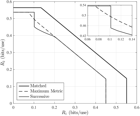
Figure 1: Achievable rate regions for the standard MAC given in (21) with mismatched successive decoding and mismatched maximum-metric decoding.

Interestingly, neither of the mismatched rate regions is included in the other, thus suggesting that the two decoding rules are fundamentally different. For the given input distribution, the sum rate for successive decoding exceeds that of maximum-metric decoding. Furthermore, upon taking the convex hull (which is justified by a time sharing argument), the region for successive decoding is strictly larger. While we observed similar behaviors for other choices of $Q_{1}$ and $Q_{2}$, it remains unclear as to whether this is always the case. Furthermore, while the rate region for maximum-metric decoding is tight with respect to the ensemble average, it is unclear whether the same is true of the region given in Theorem 1.

To gain insight into the shape of the achievable rate region for successive decoding, it is instructive to consider the various parts of the region. When doing so, the reader may wish to note that the condition in (16) can equivalently be expressed as three related conditions holding simultaneously; see Appendix B, leading to the conditions (128), (130), and (135). We have the following:

• The horizontal line at $R_{2}\approx 0.54$ corresponds to the requirement on $R_{2}$ in (17), which is identical to the condition in (7) for maximum-metric decoding.

• The vertical line at $R_{1}\approx 0.45$ also coincides with a condition for maximum-metric decoding, namely, (6). It is unsurprising that the two rate regions coincide at $R_{2}=0$, since if user 2 only has one message then the two decoding rules are identical. For small but positive $R_{2}$, the rate region boundaries still coincide even though the decoding rules differ, and the successive decoding curve is dominated by condition (135) in Appendix B.

• The straight diagonal part of the achievable rate region also matches that of maximum-metric decoding. In this case, the successive decoding curve is dominated by condition (130) in Appendix B; the term $\max\{0,I_{\widetilde{P}^{\prime}}(X_{2};X_{1},Y)-R_{2}\}$ expressed by the $[\cdot]^{+}$ function is dominated by $I_{\widetilde{P}^{\prime}}(X_{2};X_{1},Y)-R_{2}$, and the overall condition becomes a sum-rate bound, i.e., an upper bound on $R_{1}+R_{2}$.

• In the remaining part of the curve, as $R_{1}$ gets smaller, the rate region boundary bends downwards, and then suddenly becomes vertical. In this part, the successive decoding curve is dominated by (128) in Appendix B, with $R_{2}$ being large enough for the term $\max\{0,I_{\widetilde{P}^{\prime}}(X_{2};X_{1},Y)-R_{2}\}$ to equal zero. The step-like behavior at $R_{1}\approx 0.1$ corresponds to a change in the dominant term of $\underline{F}$ (see (14)); in the non-vertical part, the dominant term is $\mathbb{E}_{\widetilde{P}}[\log q(X_{1},X_{2},Y)]$, whereas in the vertical part, $R_{2}$ is large enough for the other term to dominate.

It is worth noting that under optimal decoding for the interference channel (which takes the form (2)), it is known that for $R_{1}$ below a certain threshold, $R_{2}$ can be arbitrarily large while still ensuring that user 1’s message is estimated correctly [26]. This is in analogy with the step-like behavior observed in Figure 1.

Finally, we note that the mismatched maximum-metric decoding region also has a non-pentagonal and non-convex shape (see the zoomed part of Figure 1), though its deviation from the usual pentagonal shape is milder than the successive decoder in this example.

II-B Cognitive MAC

In this section, we consider the analog of Theorem 1 for the cognitive MAC. Besides being of interest in its own right, this will provide a case where ensemble-tightness can be established, and with the numerical results still exhibiting similar phenomena to those shown in Figure 1.

We again begin by introducing the random coding ensemble. We fix a joint distribution $Q_{X_{1}X_{2}}\in\mathcal{P}(\mathcal{X}_{1}\times\mathcal{X}_{2})$, let $Q_{X_{1}X_{2},n}$ be the corresponding closest joint type in the same way as the previous subsection, and write the resulting marginals as $Q_{X_{1}}$, $Q_{X_{1},n}$, $Q_{X_{2}|X_{1}}$, $Q_{X_{2}|X_{1},n}$, and so on. We consider superposition coding, treating user 1’s messages as the “cloud centers”, and user 2’s messages as the “satellite codewords”. More precisely, defining

$$P_{\boldsymbol{X}_{1}}(\boldsymbol{x}_{1}) =\frac{1}{|T^{n}(Q_{X_{1},n})|}\mathds{1}\big{\{}\boldsymbol{x}_{1}\in T^{n}(Q_{X_{1},n})\big{\}},$$ (22)

$$P_{\boldsymbol{X}_{2}|\boldsymbol{X}_{1}}(\boldsymbol{x}_{2}|\boldsymbol{x}_{1}) =\frac{1}{|T^{n}_{\boldsymbol{x}_{1}}(Q_{X_{2}|X_{1},n})|}\mathds{1}\big{\{}\boldsymbol{x}_{2}\in T^{n}_{\boldsymbol{x}_{1}}(Q_{X_{2}|X_{1},n})\big{\}},$$ (23)

the codewords are distributed as follows:

$$\bigg{\{}\Big{(}\boldsymbol{X}_{1}^{(i)},\{\boldsymbol{X}_{2}^{(i,j)}\}_{j=1}^{M_{2}}\Big{)}\bigg{\}}_{i=1}^{M_{1}}\,\sim\,\prod_{i=1}^{M_{1}}\bigg{(}P_{\boldsymbol{X}_{1}}(\boldsymbol{x}_{1}^{(i)})\prod_{j=1}^{M_{2}}P_{\boldsymbol{X}_{2}|\boldsymbol{X}_{1}}(\boldsymbol{x}_{2}^{(i,j)}|\boldsymbol{x}_{1}^{(i)})\bigg{)}.$$ (24)

For the remaining definitions, we use similar notation to the standard MAC, with an additional subscript to avoid confusion. The analogous quantities to (13)–(15) are

$$\mkern 1.25mu\overline{\mkern-1.25muF\mkern-0.25mu}\mkern 0.25mu_{\mathrm{c}}(\widetilde{P}_{X_{1}X_{2}Y}^{\prime},R_{2}) \triangleq\mathbb{E}_{\widetilde{P}^{\prime}}[\log q(X_{1},X_{2},Y)]+\big{[}R_{2}-I_{\widetilde{P}^{\prime}}(X_{2};Y|X_{1})\big{]}^{+},$$ (25)

$$\underline{F}_{\mathrm{c}}(P_{X_{1}X_{2}Y},R_{2}) \triangleq\max\bigg{\{}\mathbb{E}_{P}[\log q(X_{1},X_{2},Y)],$$

$$\max_{P_{X_{1}X_{2}Y}^{\prime}\in\mathcal{T}^{\prime}_{1\mathrm{c}}(P_{X_{1}X_{2}Y},R_{2})}\mathbb{E}_{P^{\prime}}[\log q(X_{1},X_{2},Y)]+R_{2}-I_{P^{\prime}}(X_{2};Y|X_{1})\bigg{\}},$$ (26)

where

$$\mathcal{T}^{\prime}_{1\mathrm{c}}(P_{X_{1}X_{2}Y},R_{2}) \triangleq\Big{\{}P_{X_{1}X_{2}Y}^{\prime}\,:\,P_{X_{1}Y}^{\prime}=P_{X_{1}Y},P_{X_{1}X_{2}}^{\prime}=P_{X_{1}X_{2}},I_{P^{\prime}}(X_{2};Y|X_{1})\leq R_{2}\Big{\}}.$$ (27)

Our main result for the cognitive MAC is as follows.

Theorem 2.

For any input distribution $Q_{X_{1}X_{2}}$, the pair $(R_{1},R_{2})$ is achievable for the cognitive MAC with the mismatched successive decoding rule in (2)–(3) provided that

$$R_{1} \leq\min_{\widetilde{P}_{X_{1}X_{2}Y}^{\prime}\in\mathcal{T}_{1\mathrm{c}}(Q_{X_{1}X_{2}}\times W,R_{2})}I_{\widetilde{P}^{\prime}}(X_{1};Y)+\big{[}I_{\widetilde{P}^{\prime}}(X_{2};Y|X_{1})-R_{2}\big{]}^{+}$$ (28)

$$R_{2} \leq\min_{\widetilde{P}_{X_{1}X_{2}Y}\in\mathcal{T}_{2\mathrm{c}}(Q_{X_{1}X_{2}}\times W)}I_{\widetilde{P}}(X_{2};Y|X_{1}),$$ (29)

where

$$\mathcal{T}_{1\mathrm{c}}(P_{X_{1}X_{2}Y},R_{2}) \triangleq\Big{\{}\widetilde{P}_{X_{1}X_{2}Y}^{\prime}\,:\,P_{X_{1}X_{2}}^{\prime}=P_{X_{1}X_{2}},\widetilde{P}^{\prime}_{Y}=P_{Y},\mkern 1.25mu\overline{\mkern-1.25muF\mkern-0.25mu}\mkern 0.25mu_{\mathrm{c}}(\widetilde{P}_{X_{1}X_{2}Y}^{\prime},R_{2})\geq\underline{F}_{\mathrm{c}}(P_{X_{1}X_{2}Y},R_{2})\Big{\}},$$ (30)

$$\mathcal{T}_{2\mathrm{c}}(P_{X_{1}X_{2}Y}) \triangleq\Big{\{}\widetilde{P}_{X_{1}X_{2}Y}\,:\,\widetilde{P}_{X_{1}X_{2}}=P_{X_{1}X_{2}},\widetilde{P}_{X_{1}Y}=P_{X_{1}Y},$$

$$\qquad\qquad\qquad\qquad\mathbb{E}_{\widetilde{P}}[\log q(X_{1},X_{2},Y)]\geq\mathbb{E}_{P}[\log q(X_{1},X_{2},Y)]\Big{\}}.$$ (31)

Conversely, for any rate pair $(R_{1},R_{2})$ failing to meet both of (28)–(29), the random-coding error probability resulting from (22)–(24) tends to one as $n\to\infty$.

Proof.

See Section IV. ∎

In Appendix B, we cast (28) in terms of convex optimization problems. Similarly to the previous subsection, the exponent corresponding to (29) is precisely that corresponding to the second user in [4, Thm. 1], and the exponent corresponding to (28) is given by

$$\min_{P_{X_{1}X_{2}Y}\,:\,P_{X_{1}X_{2}}=Q_{X_{1}X_{2}}}D(P_{X_{1}X_{2}Y}\|Q_{X_{1}X_{2}}\times W)+\big{[}I_{0\mathrm{c}}(P_{X_{1}X_{2}Y},R_{2})-R_{1}\big{]}^{+},$$ (32)

where $I_{0\mathrm{c}}(P_{X_{1}X_{2}Y},R_{2})$ denotes the right-hand side of (28) with an arbitrary distribution $P_{X_{1}X_{2}Y}$ in place of $Q_{X_{1}X_{2}}\times W$. Similarly to the rate region, the proof of Theorem 2 shows that these exponents are tight with respect to the ensemble average (sometimes referred to as exact random-coding exponents [27]).

Numerical Example

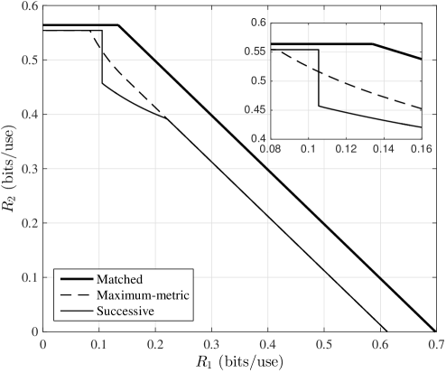
Figure 2: Achievable rate regions for the cognitive MAC given in (21) with mismatched successive decoding and mismatched maximum-metric decoding.

We consider again consider the transition law (and the corresponding decoding metric with a single value of $\delta$) given in (21) with $\delta_{00}=0.01$, $\delta_{01}=0.1$, $\delta_{10}=0.01$, $\delta_{11}=0.3$, $\delta=0.15$, and $Q_{X_{1}X_{2}}=Q_{1}\times Q_{2}$ with $Q_{1}=Q_{2}=(0.5,0.5)$. Figure 2 plots the achievable rates regions of successive decoding (Theorem 2), maximum-metric decoding ((9)–(10)), and matched decoding (again yielding the same region whether successive or maximum-metric, cf. Appendix A).

We see that the behavior of the decoders is completely analogous to the non-cognitive case observed in Figure 1. The key difference here is that we know that all three regions are tight with respect to the ensemble average. Thus, we may conclude that the somewhat unusual shape of the region for successive decoding is not merely an artifact of our analysis, but it is indeed inherent to the random-coding ensemble and the decoder.

III Proof of Theorem 1

The proof of Theorem 1 is based on the method of type class enumeration (e.g. see [26, 28, 27]), and is perhaps most similar to that of Somekh-Baruch and Merhav [27].

Step 1: Initial Bound

We assume without loss of generality that $\mathsf{m}_{1}=\mathsf{m}_{2}=1$, and we write $\boldsymbol{X}_{\nu}=\boldsymbol{X}_{\nu}^{(1)}$ and let $\mkern 3.5mu\overline{\mkern-3.5mu\boldsymbol{X}\mkern-0.75mu}\mkern 0.75mu_{\nu}$ denote an arbitrary codeword $\boldsymbol{X}_{\nu}^{(j)}$ with $j\neq 1$. Thus,

$$(\boldsymbol{X}_{1},\boldsymbol{X}_{2},\boldsymbol{Y},\mkern 3.5mu\overline{\mkern-3.5mu\boldsymbol{X}\mkern-0.75mu}\mkern 0.75mu_{1},\mkern 3.5mu\overline{\mkern-3.5mu\boldsymbol{X}\mkern-0.75mu}\mkern 0.75mu_{2})\sim P_{\boldsymbol{X}_{1}}(\boldsymbol{x}_{1})P_{\boldsymbol{X}_{2}}(\boldsymbol{x}_{2})W^{n}(\boldsymbol{y}|\boldsymbol{x}_{1},\boldsymbol{x}_{2})P_{\boldsymbol{X}_{1}}(\mkern 1.25mu\overline{\mkern-1.25mu\boldsymbol{x}\mkern-0.25mu}\mkern 0.25mu_{1})P_{\boldsymbol{X}_{2}}(\mkern 1.25mu\overline{\mkern-1.25mu\boldsymbol{x}\mkern-0.25mu}\mkern 0.25mu_{2}).$$ (33)

We define the following error events:

(Type 1)	$\sum_{j}q^{n}(\boldsymbol{X}_{1}^{(i)},\boldsymbol{X}_{2}^{(j)},\boldsymbol{Y})\geq\sum_{j}q^{n}(\boldsymbol{X}_{1},\boldsymbol{X}_{2}^{(j)},\boldsymbol{Y})$ for some $i\neq 1$;
(Type 2)	$q^{n}(\boldsymbol{X}_{1},\boldsymbol{X}_{2}^{(j)},\boldsymbol{Y})\geq q^{n}(\boldsymbol{X}_{1},\boldsymbol{X}_{2},\boldsymbol{Y})$ for some $j\neq 1$.

Denoting the probabilities of these events by $\mkern 1.25mu\overline{\mkern-1.25mup\mkern-0.25mu}\mkern 0.25mu_{\mathrm{e},1}$ and $\mkern 1.25mu\overline{\mkern-1.25mup\mkern-0.25mu}\mkern 0.25mu_{\mathrm{e},2}$ respectively, it follows that the overall random-coding error probability $\mkern 1.25mu\overline{\mkern-1.25mup\mkern-0.25mu}\mkern 0.25mu_{\mathrm{e}}$ is upper bounded by $\mkern 1.25mu\overline{\mkern-1.25mup\mkern-0.25mu}\mkern 0.25mu_{\mathrm{e},1}+\mkern 1.25mu\overline{\mkern-1.25mup\mkern-0.25mu}\mkern 0.25mu_{\mathrm{e},2}$.

The analysis of the type-2 error event is precisely that of one of the three error types for maximum-metric decoding [3, 5], yielding the rate condition in (17). We thus focus on the type-1 event. We let $\mkern 1.25mu\overline{\mkern-1.25mup\mkern-0.25mu}\mkern 0.25mu_{\mathrm{e},1}(\boldsymbol{x}_{1},\boldsymbol{x}_{2},\boldsymbol{y})$ denote the probability of the type-1 event conditioned on $(\boldsymbol{X}_{1}^{(1)},\boldsymbol{X}_{2}^{(1)},\boldsymbol{Y})=(\boldsymbol{x}_{1},\boldsymbol{x}_{2},\boldsymbol{y})$, and we denote the joint type of $(\boldsymbol{x}_{1},\boldsymbol{x}_{2},\boldsymbol{y})$ by $P_{X_{1}X_{2}Y}$. We write the objective function in (2) as

$$\Xi_{\boldsymbol{x}_{2}\boldsymbol{y}}(\mkern 1.25mu\overline{\mkern-1.25mu\boldsymbol{x}\mkern-0.25mu}\mkern 0.25mu_{1})\triangleq q^{n}(\mkern 1.25mu\overline{\mkern-1.25mu\boldsymbol{x}\mkern-0.25mu}\mkern 0.25mu_{1},\boldsymbol{x}_{2},\boldsymbol{y})+\sum_{j\neq 1}q^{n}(\mkern 1.25mu\overline{\mkern-1.25mu\boldsymbol{x}\mkern-0.25mu}\mkern 0.25mu_{1},\boldsymbol{X}_{2}^{(j)},\boldsymbol{y}).$$ (34)

This quantity is random due to the randomness of $\{\boldsymbol{X}_{2}^{(j)}\}$. The starting point of our analysis is the union bound:

$$\mkern 1.25mu\overline{\mkern-1.25mup\mkern-0.25mu}\mkern 0.25mu_{\mathrm{e},1}(\boldsymbol{x}_{1},\boldsymbol{x}_{2},\boldsymbol{y})\leq(M_{1}-1)\mathbb{P}\big{[}\Xi_{\boldsymbol{x}_{2}\boldsymbol{y}}(\mkern 3.5mu\overline{\mkern-3.5mu\boldsymbol{X}\mkern-0.75mu}\mkern 0.75mu_{1})\geq\Xi_{\boldsymbol{x}_{2}\boldsymbol{y}}(\boldsymbol{x}_{1})\big{]}.$$ (35)

The difficulty in analyzing (35) is that for two different codewords $\boldsymbol{x}_{1}$ and $\mkern 1.25mu\overline{\mkern-1.25mu\boldsymbol{x}\mkern-0.25mu}\mkern 0.25mu_{1}$, $\Xi_{\boldsymbol{x}_{2}\boldsymbol{y}}(\boldsymbol{x}_{1})$ and $\Xi_{\boldsymbol{x}_{2}\boldsymbol{y}}(\mkern 1.25mu\overline{\mkern-1.25mu\boldsymbol{x}\mkern-0.25mu}\mkern 0.25mu_{1})$ are not independent, and their joint statistics are complicated. We will circumvent this issue by conditioning on high probability events under which these random quantities can be bounded by deterministic values.

Step 2: An Auxiliary Lemma

We introduce some additional notation. For a given realization $(\boldsymbol{x}_{1},\boldsymbol{x}_{2},\boldsymbol{y})$ of $(\boldsymbol{X}_{1},\boldsymbol{X}_{2},\boldsymbol{Y})$, we let $\widetilde{P}_{X_{1}X_{2}Y}$ denote its joint type and we write $q^{n}(\widetilde{P}_{X_{1}X_{2}Y}^{\prime})\triangleq q^{n}(\mkern 1.25mu\overline{\mkern-1.25mu\boldsymbol{x}\mkern-0.25mu}\mkern 0.25mu_{1},\mkern 1.25mu\overline{\mkern-1.25mu\boldsymbol{x}\mkern-0.25mu}\mkern 0.25mu_{2},\boldsymbol{y})$. In addition, for a general sequence $\mkern 1.25mu\overline{\mkern-1.25mu\boldsymbol{x}\mkern-0.25mu}\mkern 0.25mu_{1}$, we define the type enumerator

$$N_{\mkern 1.25mu\overline{\mkern-1.25mu\boldsymbol{x}\mkern-0.25mu}\mkern 0.25mu_{1}\boldsymbol{y}}(\widetilde{P}_{X_{1}X_{2}Y}^{\prime})=\sum_{j\neq 1}\mathds{1}\Big{\{}(\mkern 1.25mu\overline{\mkern-1.25mu\boldsymbol{x}\mkern-0.25mu}\mkern 0.25mu_{1},\boldsymbol{X}_{2}^{(j)},\boldsymbol{y})\in T^{n}(\widetilde{P}_{X_{1}X_{2}Y}^{\prime})\Big{\}},$$ (36)

which represents the random number of $\boldsymbol{X}_{2}^{(j)}$ $(j\neq 1)$ such that $(\mkern 1.25mu\overline{\mkern-1.25mu\boldsymbol{x}\mkern-0.25mu}\mkern 0.25mu_{1},\boldsymbol{X}_{2}^{(j)},\boldsymbol{y})\in T^{n}(\widetilde{P}_{X_{1}X_{2}Y}^{\prime})$. As we will see below, when $\mkern 3.5mu\overline{\mkern-3.5mu\boldsymbol{X}\mkern-0.75mu}\mkern 0.75mu_{1}=\mkern 1.25mu\overline{\mkern-1.25mu\boldsymbol{x}\mkern-0.25mu}\mkern 0.25mu_{1}$, the quantity $\Xi_{\boldsymbol{x}_{2}\boldsymbol{y}}(\mkern 1.25mu\overline{\mkern-1.25mu\boldsymbol{x}\mkern-0.25mu}\mkern 0.25mu_{1})$ can be re-written in terms of $N_{\mkern 1.25mu\overline{\mkern-1.25mu\boldsymbol{x}\mkern-0.25mu}\mkern 0.25mu_{1}\boldsymbol{y}}(\cdot)$, and $\Xi_{\boldsymbol{x}_{2}\boldsymbol{y}}(\boldsymbol{x}_{1})$ can similarly be re-written in terms of $N_{\boldsymbol{x}_{1}\boldsymbol{y}}(\cdot)$.

The key to replacing random quantities by deterministic ones is to condition on events that hold with probability one approaching faster than exponentially, thus not affecting the exponential behavior of interest. The following lemma will be used for this purpose, characterizing the behavior of $N_{\mkern 1.25mu\overline{\mkern-1.25mu\boldsymbol{x}\mkern-0.25mu}\mkern 0.25mu_{1}\boldsymbol{y}}(\widetilde{P}_{X_{1}X_{2}Y}^{\prime})$ for various choices of $R_{2}$ and $\widetilde{P}_{X_{1}X_{2}Y}^{\prime}$. The proof can be found in [26, 27], and is based on the fact that

$$\mathbb{P}\big{[}(\mkern 1.25mu\overline{\mkern-1.25mu\boldsymbol{x}\mkern-0.25mu}\mkern 0.25mu_{1},\mkern 3.5mu\overline{\mkern-3.5mu\boldsymbol{X}\mkern-0.75mu}\mkern 0.75mu_{2},\boldsymbol{y})\in T^{n}(\widetilde{P}_{X_{1}X_{2}Y}^{\prime})\big{]}\doteq e^{-nI_{\widetilde{P}^{\prime}}(X_{2};X_{1},Y)},$$ (37)

which is a standard property of types [25, Ch. 2].

Lemma 1.

[26, 27] Fix the pair $(\mkern 1.25mu\overline{\mkern-1.25mu\boldsymbol{x}\mkern-0.25mu}\mkern 0.25mu_{1},\boldsymbol{y})\in T^{n}(\widetilde{P}_{X_{1}Y})$, a constant $\delta>0$, and a type $\widetilde{P}_{X_{1}X_{2}Y}^{\prime}\in\mathcal{S}_{1,n}^{\prime}(Q_{2,n},\widetilde{P}_{X_{1}Y})$.

1. If $R_{2}\geq I_{\widetilde{P}^{\prime}}(X_{2};X_{1},Y)+\delta$, then

   $$M_{2}e^{-n(I_{\widetilde{P}^{\prime}}(X_{2};X_{1},Y)+\delta)}\leq N_{\mkern 1.25mu\overline{\mkern-1.25mu\boldsymbol{x}\mkern-0.25mu}\mkern 0.25mu_{1}\boldsymbol{y}}(\widetilde{P}_{X_{1}X_{2}Y}^{\prime})\leq M_{2}e^{-n(I_{\widetilde{P}^{\prime}}(X_{2};X_{1},Y)-\delta)}$$ (38)

   with probability approaching one faster than exponentially.

2. If $R_{2}<I_{\widetilde{P}^{\prime}}(X_{2};X_{1},Y)+\delta$, then

   $$N_{\mkern 1.25mu\overline{\mkern-1.25mu\boldsymbol{x}\mkern-0.25mu}\mkern 0.25mu_{1}\boldsymbol{y}}(\widetilde{P}_{X_{1}X_{2}Y}^{\prime})\leq e^{n\,2\delta}$$ (39)

   with probability approaching one faster than exponentially.

Roughly speaking, Lemma 1 states that if $R_{2}>I_{\widetilde{P}^{\prime}}(X_{2};X_{1},Y)$ then the type enumerator is highly concentrated about its mean, whereas if $R_{2}<I_{\widetilde{P}^{\prime}}(X_{2};X_{1},Y)$ then the type enumerator takes a subexponential value (possibly zero) with overwhelming probability.

Given a joint type $\widetilde{P}_{X_{1}Y}$, define the event

$$\mathcal{A}_{\delta}(\widetilde{P}_{X_{1}Y})= \Big{\{}\text{\eqref{eq:SUC_Lem1a} holds for all }\widetilde{P}_{X_{1}X_{2}Y}^{\prime}\in\mathcal{S}_{1,n}^{\prime}(Q_{2,n},\widetilde{P}_{X_{1}Y})\text{ with }R_{2}\geq I_{\widetilde{P}^{\prime}}(X_{2};X_{1},Y)+\delta\Big{\}}$$

$$\cap\, \Big{\{}\text{\eqref{eq:SUC_Lem1c} holds for all }\widetilde{P}_{X_{1}X_{2}Y}^{\prime}\in\mathcal{S}_{1,n}^{\prime}(Q_{2,n},\widetilde{P}_{X_{1}Y})\text{ with }R_{2}<I_{\widetilde{P}^{\prime}}(X_{2};X_{1},Y)+\delta\Big{\}},$$ (40)

where

$$\mathcal{S}_{1,n}^{\prime}(Q_{2,n},\widetilde{P}_{X_{1}Y})\triangleq\Big{\{}\widetilde{P}_{X_{1}X_{2}Y}^{\prime}\in\mathcal{P}_{n}(\mathcal{X}_{1}\times\mathcal{X}_{2}\times\mathcal{Y})\,:\,\widetilde{P}_{X_{1}Y}^{\prime}=\widetilde{P}_{X_{1}Y},\widetilde{P}_{X_{2}}^{\prime}=Q_{2,n}\Big{\}},$$ (41)

and where we recall the definition of $Q_{2,n}$ at the start of Section II-A. By Lemma 1 and the union bound, $\mathbb{P}[\mathcal{A}_{\delta}(\widetilde{P}_{X_{1}Y})]\to 1$ faster than exponentially. and hence we can safely condition any event on $\mathcal{A}_{\delta}(\widetilde{P}_{X_{1}Y})$ without changing the exponential behavior of the corresponding probability. This can be seen by writing the following for any event $\mathcal{E}$:

$$\mathbb{P}[\mathcal{E}] =\mathbb{P}[\mathcal{E}\cap\mathcal{A}]+\mathbb{P}[\mathcal{E}\cap\mathcal{A}^{c}]$$ (42)

$$\leq\mathbb{P}[\mathcal{E}\,|\,\mathcal{A}]+\mathbb{P}[\mathcal{A}^{c}],$$ (43)

$$\mathbb{P}[\mathcal{E}] \geq\mathbb{P}[\mathcal{E}\cap\mathcal{A}]$$ (44)

$$=(1-\mathbb{P}[\mathcal{A}^{c}])\mathbb{P}[\mathcal{E}\,|\,\mathcal{A}]$$ (45)

$$\geq\mathbb{P}[\mathcal{E}\,|\,\mathcal{A}]-\mathbb{P}[\mathcal{A}^{c}].$$ (46)

Using these observations, we will condition on $\mathcal{A}_{\delta}$ several times throughout the remainder of the proof.

Step 3: Bound $\Xi_{\boldsymbol{x}_{2}\boldsymbol{y}}(\boldsymbol{x}_{1})$ by a Deterministic Quantity

From (34), we have

$$\Xi_{\boldsymbol{x}_{2}\boldsymbol{y}}(\mkern 1.25mu\overline{\mkern-1.25mu\boldsymbol{x}\mkern-0.25mu}\mkern 0.25mu_{1})=q^{n}(\widetilde{P}_{X_{1}X_{2}Y})+\sum_{\widetilde{P}_{X_{1}X_{2}Y}^{\prime}}N_{\mkern 1.25mu\overline{\mkern-1.25mu\boldsymbol{x}\mkern-0.25mu}\mkern 0.25mu_{1}\boldsymbol{y}}(\widetilde{P}_{X_{1}X_{2}Y}^{\prime})q^{n}(\widetilde{P}_{X_{1}X_{2}Y}^{\prime}).$$ (47)

Since the codewords are generated independently, $N_{\mkern 1.25mu\overline{\mkern-1.25mu\boldsymbol{x}\mkern-0.25mu}\mkern 0.25mu_{1}\boldsymbol{y}}(\widetilde{P}_{X_{1}X_{2}Y}^{\prime})$ is binomially distributed with $M_{2}-1$ trials and success probability $\mathbb{P}\big{[}(\mkern 1.25mu\overline{\mkern-1.25mu\boldsymbol{x}\mkern-0.25mu}\mkern 0.25mu_{1},\mkern 3.5mu\overline{\mkern-3.5mu\boldsymbol{X}\mkern-0.75mu}\mkern 0.75mu_{2},\boldsymbol{y})\in T^{n}(\widetilde{P}_{X_{1}X_{2}Y}^{\prime})\big{]}.$ By construction, we have $N_{\mkern 1.25mu\overline{\mkern-1.25mu\boldsymbol{x}\mkern-0.25mu}\mkern 0.25mu_{1}\boldsymbol{y}}(\widetilde{P}_{X_{1}X_{2}Y}^{\prime})=0$ unless $\widetilde{P}_{X_{1}X_{2}Y}^{\prime}\in\mathcal{S}_{1,n}^{\prime}(Q_{2,n},\widetilde{P}_{X_{1}Y})$, where $\mathcal{S}_{1,n}^{\prime}$ is defined in (41).

Conditioned on $\mathcal{A}_{\delta}(P_{X_{1}Y})$, we have the following:

$$\Xi_{\boldsymbol{x}_{2}\boldsymbol{y}}(\boldsymbol{x}_{1}) =q^{n}(P_{X_{1}X_{2}Y})+\sum_{P_{X_{1}X_{2}Y}^{\prime}}N_{\boldsymbol{x}_{1}\boldsymbol{y}}(P_{X_{1}X_{2}Y}^{\prime})q^{n}(P_{X_{1}X_{2}Y}^{\prime})$$ (48)

$$\geq q^{n}(P_{X_{1}X_{2}Y})+\max_{\begin{subarray}{c}P_{X_{1}X_{2}Y}^{\prime}\in\mathcal{S}_{1,n}^{\prime}(Q_{2,n},P_{X_{1}Y})\\ R_{2}\geq I_{P^{\prime}}(X_{2};X_{1},Y)+\delta\end{subarray}}N_{\boldsymbol{x}_{1}\boldsymbol{y}}(P_{X_{1}X_{2}Y}^{\prime})q^{n}(P_{X_{1}X_{2}Y}^{\prime})$$ (49)

$$\geq q^{n}(P_{X_{1}X_{2}Y})+\max_{\begin{subarray}{c}P_{X_{1}X_{2}Y}^{\prime}\in\mathcal{S}_{1,n}^{\prime}(Q_{2,n},P_{X_{1}Y})\\ R_{2}\geq I_{P^{\prime}}(X_{2};X_{1},Y)+\delta\end{subarray}}M_{2}e^{-n(I_{P^{\prime}}(X_{2};X_{1},Y)+\delta)}q^{n}(P_{X_{1}X_{2}Y}^{\prime})$$ (50)

$$\triangleq\underline{G}_{\delta,n}(P_{X_{1}X_{2}Y}),$$ (51)

where (50) follows from (38). Unlike $\Xi_{\boldsymbol{x}_{2}\boldsymbol{y}}(\boldsymbol{x}_{1})$, the quantity $\underline{G}_{\delta,n}(P_{X_{1}X_{2}Y})$ is deterministic. Substituting (51) into (35) and using the fact that $\mathbb{P}\big{[}\mathcal{A}_{\delta}(\widetilde{P}_{X_{1}Y})\big{]}\to 1$ faster than exponentially, we obtain

$$\mkern 1.25mu\overline{\mkern-1.25mup\mkern-0.25mu}\mkern 0.25mu_{\mathrm{e},1}(\boldsymbol{x}_{1},\boldsymbol{x}_{2},\boldsymbol{y})\,\,\dot{\leq}\,M_{1}\mathbb{P}\big{[}\Xi_{\boldsymbol{x}_{2}\boldsymbol{y}}(\mkern 3.5mu\overline{\mkern-3.5mu\boldsymbol{X}\mkern-0.75mu}\mkern 0.75mu_{1})\geq\underline{G}_{\delta,n}(P_{X_{1}X_{2}Y})\big{]}.$$ (52)

Step 4: An Expansion Based on Types

Since the statistics of $\Xi_{\boldsymbol{x}_{2}\boldsymbol{y}}(\mkern 1.25mu\overline{\mkern-1.25mu\boldsymbol{x}\mkern-0.25mu}\mkern 0.25mu_{1})$ depend on $\mkern 1.25mu\overline{\mkern-1.25mu\boldsymbol{x}\mkern-0.25mu}\mkern 0.25mu_{1}$ only through the joint type of $(\mkern 1.25mu\overline{\mkern-1.25mu\boldsymbol{x}\mkern-0.25mu}\mkern 0.25mu_{1},\boldsymbol{x}_{2},\boldsymbol{y})$, we can write (52) as follows:

$$\mkern 1.25mu\overline{\mkern-1.25mup\mkern-0.25mu}\mkern 0.25mu_{\mathrm{e},1}(\boldsymbol{x}_{1},\boldsymbol{x}_{2},\boldsymbol{y}) \,\,\dot{\leq}\,M_{1}\sum_{\widetilde{P}_{X_{1}X_{2}Y}}\mathbb{P}\big{[}(\mkern 3.5mu\overline{\mkern-3.5mu\boldsymbol{X}\mkern-0.75mu}\mkern 0.75mu_{1},\boldsymbol{x}_{2},\boldsymbol{y})\in T^{n}(\widetilde{P}_{X_{1}X_{2}Y})\big{]}\mathbb{P}\big{[}\Xi_{\boldsymbol{x}_{2}\boldsymbol{y}}(\mkern 1.25mu\overline{\mkern-1.25mu\boldsymbol{x}\mkern-0.25mu}\mkern 0.25mu_{1})\geq\underline{G}_{\delta,n}(P_{X_{1}X_{2}Y})\big{]}$$ (53)

$$\doteq M_{1}\max_{\widetilde{P}_{X_{1}X_{2}Y}\in\mathcal{S}_{1,n}(Q_{1,n},P_{X_{2}Y})}e^{-nI_{\widetilde{P}}(X_{1};X_{2},Y)}\mathbb{P}\big{[}\Xi_{\boldsymbol{x}_{2}\boldsymbol{y}}(\mkern 1.25mu\overline{\mkern-1.25mu\boldsymbol{x}\mkern-0.25mu}\mkern 0.25mu_{1})\geq\underline{G}_{\delta,n}(P_{X_{1}X_{2}Y})\big{]},$$ (54)

where $\mkern 1.25mu\overline{\mkern-1.25mu\boldsymbol{x}\mkern-0.25mu}\mkern 0.25mu_{1}$ denotes an arbitrary sequence such that $(\mkern 1.25mu\overline{\mkern-1.25mu\boldsymbol{x}\mkern-0.25mu}\mkern 0.25mu_{1},\boldsymbol{x}_{2},\boldsymbol{y})\in T^{n}(\widetilde{P}_{X_{1}X_{2}Y})$, and

$$\mathcal{S}_{1,n}(Q_{1,n},P_{X_{2}Y})\triangleq\Big{\{}\widetilde{P}_{X_{1}X_{2}Y}\in\mathcal{P}_{n}(\mathcal{X}_{1}\times\mathcal{X}_{2}\times\mathcal{Y})\,:\,\widetilde{P}_{X_{1}}=Q_{1,n},\widetilde{P}_{X_{2}Y}=P_{X_{2}Y}\Big{\}}.$$ (55)

In (54), we have used an analogous property to (37) and the fact that by construction, the joint type of $(\mkern 3.5mu\overline{\mkern-3.5mu\boldsymbol{X}\mkern-0.75mu}\mkern 0.75mu_{1},\boldsymbol{x}_{2},\boldsymbol{y})$ is in $\mathcal{S}_{1,n}(Q_{1,n},P_{X_{2}Y})$ with probability one.

Step 5: Bound $\Xi_{\boldsymbol{x}_{2}\boldsymbol{y}}(\mkern 1.25mu\overline{\mkern-1.25mu\boldsymbol{x}\mkern-0.25mu}\mkern 0.25mu_{1})$ by a Deterministic Quantity

Next, we again use Lemma 1 in order to replace $\Xi_{\boldsymbol{x}_{2}\boldsymbol{y}}(\mkern 1.25mu\overline{\mkern-1.25mu\boldsymbol{x}\mkern-0.25mu}\mkern 0.25mu_{1})$ in (54) by a deterministic quantity. We have from (47) that

$$\Xi_{\boldsymbol{x}_{2}\boldsymbol{y}}(\mkern 1.25mu\overline{\mkern-1.25mu\boldsymbol{x}\mkern-0.25mu}\mkern 0.25mu_{1})\leq q^{n}(\widetilde{P}_{X_{1}X_{2}Y})+p_{0}(n)\max_{\widetilde{P}_{X_{1}X_{2}Y}^{\prime}}N_{\mkern 1.25mu\overline{\mkern-1.25mu\boldsymbol{x}\mkern-0.25mu}\mkern 0.25mu_{1}\boldsymbol{y}}(\widetilde{P}_{X_{1}X_{2}Y}^{\prime})q^{n}(\widetilde{P}_{X_{1}X_{2}Y}^{\prime}),$$ (56)

where $p_{0}(n)$ is a polynomial corresponding to the total number of joint types. Substituting (56) into (54), we obtain

$$\mkern 1.25mu\overline{\mkern-1.25mup\mkern-0.25mu}\mkern 0.25mu_{\mathrm{e},1}(\boldsymbol{x}_{1},\boldsymbol{x}_{2},\boldsymbol{y})\,\,\dot{\leq}\,M_{1}\max_{\widetilde{P}_{X_{1}X_{2}Y}\in\mathcal{S}_{1,n}(Q_{1,n},P_{X_{2}Y})}\max_{\widetilde{P}_{X_{1}X_{2}Y}^{\prime}\in\mathcal{S}_{1}^{\prime}(Q_{2,n},\widetilde{P}_{X_{1}Y})}e^{-nI_{\widetilde{P}}(X_{1};X_{2},Y)}\mathbb{P}\big{[}\mathcal{E}_{P,\widetilde{P}}(\widetilde{P}_{X_{1}X_{2}Y}^{\prime})\big{]},$$ (57)

where

$$\mathcal{E}_{P,\widetilde{P}}(\widetilde{P}_{X_{1}X_{2}Y}^{\prime})\triangleq\Big{\{}q^{n}(\widetilde{P}_{X_{1}X_{2}Y})+p_{0}(n)N_{\mkern 1.25mu\overline{\mkern-1.25mu\boldsymbol{x}\mkern-0.25mu}\mkern 0.25mu_{1}\boldsymbol{y}}(\widetilde{P}_{X_{1}X_{2}Y}^{\prime})q^{n}(\widetilde{P}_{X_{1}X_{2}Y}^{\prime})\geq\underline{G}_{\delta,n}(P_{X_{1}X_{2}Y})\Big{\}},$$ (58)

and we have used the union bound to take the maximum over $\widetilde{P}_{X_{1}X_{2}Y}^{\prime}$ outside the probability in (57). Continuing, we have for any $\widetilde{P}_{X_{1}X_{2}Y}\in\mathcal{S}_{1,n}(Q_{1,n},P_{X_{2}Y})$ that

$$\max_{\widetilde{P}_{X_{1}X_{2}Y}^{\prime}\in\mathcal{S}_{1,n}^{\prime}(Q_{2,n},\widetilde{P}_{X_{1}Y})}\mathbb{P}\big{[}\mathcal{E}_{P,\widetilde{P}}(\widetilde{P}_{X_{1}X_{2}Y}^{\prime})\big{]}=\max\bigg{\{} \max_{\begin{subarray}{c}\widetilde{P}_{X_{1}X_{2}Y}^{\prime}\in\mathcal{S}_{1,n}^{\prime}(Q_{2,n},\widetilde{P}_{X_{1}Y})\\ R_{2}\geq I_{\widetilde{P}^{\prime}}(X_{2};X_{1},Y)+\delta\end{subarray}}\mathbb{P}\big{[}\mathcal{E}_{P,\widetilde{P}}(\widetilde{P}_{X_{1}X_{2}Y}^{\prime})\big{]},$$

$$\max_{\begin{subarray}{c}\widetilde{P}_{X_{1}X_{2}Y}^{\prime}\in\mathcal{S}_{1,n}^{\prime}(Q_{2,n},\widetilde{P}_{X_{1}Y})\\ R_{2}<I_{\widetilde{P}^{\prime}}(X_{2};X_{1},Y)+\delta\end{subarray}}\mathbb{P}\big{[}\mathcal{E}_{P,\widetilde{P}}(\widetilde{P}_{X_{1}X_{2}Y}^{\prime})\big{]}\bigg{\}}.$$ (59)

Step 5a – Simplify the First Term

For the first term on the right-hand side of (59), observe that conditioned on $\mathcal{A}_{\delta}(\widetilde{P}_{X_{1}Y})$ in (40), we have for $\widetilde{P}_{X_{1}X_{2}Y}^{\prime}$ satisfying $R_{2}\geq I_{\widetilde{P}^{\prime}}(X_{2};X_{1},Y)+\delta$ that

$$N_{\mkern 1.25mu\overline{\mkern-1.25mu\boldsymbol{x}\mkern-0.25mu}\mkern 0.25mu_{1}\boldsymbol{y}}(\widetilde{P}_{X_{1}X_{2}Y}^{\prime})q^{n}(\widetilde{P}_{X_{1}X_{2}Y}^{\prime})\leq M_{2}e^{-n(I_{\widetilde{P}^{\prime}}(X_{2};X_{1},Y)-\delta)}q^{n}(\widetilde{P}_{X_{1}X_{2}Y}^{\prime}),$$ (60)

where we have used (38). Hence, and since $\mathbb{P}\big{[}\mathcal{A}_{\delta}(\widetilde{P}_{X_{1}Y})\big{]}\to 1$ faster than exponentially, we have

$$\mathbb{P}\big{[}\mathcal{E}_{P,\widetilde{P}}(\widetilde{P}_{X_{1}X_{2}Y}^{\prime})\big{]}\,\,\dot{\leq}\,\mathds{1}\Big{\{}q^{n}(\widetilde{P}_{X_{1}X_{2}Y})+M_{2}p_{0}(n)e^{-n(I_{\widetilde{P}^{\prime}}(X_{2};X_{1},Y)-\delta)}q^{n}(\widetilde{P}_{X_{1}X_{2}Y}^{\prime})\geq\underline{G}_{\delta,n}(P_{X_{1}X_{2}Y})\Big{\}}.$$ (61)

Step 5b – Simplify the Second Term

For the second term on the right-hand side of (59), we define the event $\mathcal{B}\triangleq\big{\{}N_{\mkern 1.25mu\overline{\mkern-1.25mu\boldsymbol{x}\mkern-0.25mu}\mkern 0.25mu_{1}\boldsymbol{y}}(\widetilde{P}_{X_{1}X_{2}Y}^{\prime})>0\big{\}}$, yielding

$$\mathbb{P}[\mathcal{B}]\,\,\dot{\leq}\,M_{2}e^{-nI_{\widetilde{P}^{\prime}}(X_{2};X_{1},Y)},$$ (62)

which follows from the union bound and (37). Whenever $R_{2}<I_{\widetilde{P}^{\prime}}(X_{2};X_{1},Y)+\delta$, we have

$$\mathbb{P}\big{[}\mathcal{E}_{P,\widetilde{P}}(\widetilde{P}_{X_{1}X_{2}Y}^{\prime})\big{]}$$

$$\leq\mathbb{P}\big{[}\mathcal{E}_{P,\widetilde{P}}(\widetilde{P}_{X_{1}X_{2}Y}^{\prime})\,\big{|}\,\mathcal{B}^{c}\big{]}+\mathbb{P}[\mathcal{B}]\mathbb{P}\big{[}\mathcal{E}_{P,\widetilde{P}}(\widetilde{P}_{X_{1}X_{2}Y}^{\prime})\,\big{|}\,\mathcal{B}\big{]}$$ (63)

$$\,\,\dot{\leq}\,\mathds{1}\big{\{}q^{n}(\widetilde{P}_{X_{1}X_{2}Y})\geq\underline{G}_{\delta,n}(P_{X_{1}X_{2}Y})\big{\}}+M_{2}e^{-nI_{\widetilde{P}^{\prime}}(X_{2};X_{1},Y)}\mathbb{P}\big{[}\mathcal{E}_{P,\widetilde{P}}(\widetilde{P}_{X_{1}X_{2}Y}^{\prime})\,\big{|}\,\mathcal{B}\big{]},$$ (64)

$$\,\,\dot{\leq}\,\mathds{1}\big{\{}q^{n}(\widetilde{P}_{X_{1}X_{2}Y})\geq\underline{G}_{\delta,n}(P_{X_{1}X_{2}Y})\big{\}}$$

$$\,\,\,\,+M_{2}e^{-nI_{\widetilde{P}^{\prime}}(X_{2};X_{1},Y)}\mathds{1}\big{\{}q^{n}(\widetilde{P}_{X_{1}X_{2}Y})+p_{0}(n)e^{n\,2\delta}q^{n}(\widetilde{P}_{X_{1}X_{2}Y}^{\prime})\geq\underline{G}_{\delta,n}(P_{X_{1}X_{2}Y})\big{\}},$$ (65)

where (64) follows using (62) and (58) along with the fact that $\mathcal{B}^{c}$ implies $N_{\mkern 1.25mu\overline{\mkern-1.25mu\boldsymbol{x}\mkern-0.25mu}\mkern 0.25mu_{1}\boldsymbol{y}}(\widetilde{P}_{X_{1}X_{2}Y}^{\prime})=0$, and (65) follows by conditioning on $\mathcal{A}_{\delta}(\widetilde{P}_{X_{1}Y})$ and using (39).

Step 6: Deduce the Exponent for Fixed $(\boldsymbol{x}_{1},\boldsymbol{x}_{2},\boldsymbol{y})$

Observe that $\underline{F}(P_{X_{1}X_{2}Y},R_{2})$ in (14) equals the exponent of $\underline{G}_{\delta,n}$ in (51) in the limit as $\delta\to 0$ and $n\to\infty$. Similarly, the exponents corresponding to the other quantities appearing in the indicator functions in (61) and (65) tend toward the following:

$$\mkern 1.25mu\overline{\mkern-1.25muF\mkern-0.25mu}\mkern 0.25mu_{1}(\widetilde{P}_{X_{1}X_{2}Y},\widetilde{P}_{X_{1}X_{2}Y}^{\prime},R_{2}) \triangleq\max\Big{\{}\mathbb{E}_{\widetilde{P}}[\log q(X_{1},X_{2},Y)],$$

$$\qquad\qquad\mathbb{E}_{\widetilde{P}^{\prime}}[\log q(X_{1},X_{2},Y)]+R_{2}-I_{\widetilde{P}^{\prime}}(X_{2};X_{1},Y)\Big{\}},$$ (66)

$$\mkern 1.25mu\overline{\mkern-1.25muF\mkern-0.25mu}\mkern 0.25mu_{2}(\widetilde{P}_{X_{1}X_{2}Y},\widetilde{P}_{X_{1}X_{2}Y}^{\prime}) \triangleq\max\Big{\{}\mathbb{E}_{\widetilde{P}}[\log q(X_{1},X_{2},Y)],\mathbb{E}_{\widetilde{P}^{\prime}}[\log q(X_{1},X_{2},Y)]\Big{\}}.$$ (67)

We claim that combining these expressions with (57), (59), (61) and (65) and taking $\delta\to 0$ (e.g., analogously to [4, p. 737], we may set $\delta=n^{-1/2}$), gives the following:

$$\mkern 1.25mu\overline{\mkern-1.25mup\mkern-0.25mu}\mkern 0.25mu_{\mathrm{e},1}(\boldsymbol{x}_{1},\boldsymbol{x}_{2},\boldsymbol{y})\,\,\dot{\leq}\,\max\Bigg{\{}\max_{\begin{subarray}{c}(\widetilde{P}_{X_{1}X_{2}Y},\widetilde{P}_{X_{1}X_{2}Y}^{\prime})\in\mathcal{T}_{1}^{(1)}(P_{X_{1}X_{2}Y},R_{2})\end{subarray}}M_{1}e^{-nI_{\widetilde{P}}(X_{1};X_{2},Y)},$$

$$\qquad\qquad\max_{\begin{subarray}{c}(\widetilde{P}_{X_{1}X_{2}Y},\widetilde{P}_{X_{1}X_{2}Y}^{\prime})\in\mathcal{T}_{1}^{(2)}(P_{X_{1}X_{2}Y},R_{2})\end{subarray}}M_{1}e^{-nI_{\widetilde{P}}(X_{1};X_{2},Y)}M_{2}e^{-nI_{\widetilde{P}^{\prime}}(X_{2};X_{1},Y)}\Bigg{\}},$$ (68)

where

$$\mathcal{T}_{1}^{(1)}(P_{X_{1}X_{2}Y},R_{2})\triangleq\Big{\{}(\widetilde{P}_{X_{1}X_{2}Y},\widetilde{P}_{X_{1}X_{2}Y}^{\prime})\,:\,\widetilde{P}_{X_{1}X_{2}Y}\in\mathcal{S}_{1}(Q_{1},P_{X_{2}Y}),\\ \widetilde{P}_{X_{1}X_{2}Y}^{\prime}\in\mathcal{S}_{1}^{\prime}(Q_{2},\widetilde{P}_{X_{1}Y}),I_{\widetilde{P}^{\prime}}(X_{2};X_{1},Y)\leq R_{2},\mkern 1.25mu\overline{\mkern-1.25muF\mkern-0.25mu}\mkern 0.25mu_{1}(\widetilde{P}_{X_{1}X_{2}Y},\widetilde{P}_{X_{1}X_{2}Y}^{\prime},R_{2})\geq\underline{F}(P_{X_{1}X_{2}Y},R_{2})\Big{\}},$$ (69)

$$\mathcal{T}_{1}^{(2)}(P_{X_{1}X_{2}Y},R_{2})\triangleq\Big{\{}(\widetilde{P}_{X_{1}X_{2}Y},\widetilde{P}_{X_{1}X_{2}Y}^{\prime})\,:\,\widetilde{P}_{X_{1}X_{2}Y}\in\mathcal{S}_{1}(Q_{1},P_{X_{2}Y}),\\ \widetilde{P}_{X_{1}X_{2}Y}^{\prime}\in\mathcal{S}_{1}^{\prime}(Q_{2},\widetilde{P}_{X_{1}Y}),I_{\widetilde{P}^{\prime}}(X_{2};X_{1},Y)\geq R_{2},\mkern 1.25mu\overline{\mkern-1.25muF\mkern-0.25mu}\mkern 0.25mu_{2}(\widetilde{P}_{X_{1}X_{2}Y},\widetilde{P}_{X_{1}X_{2}Y}^{\prime})\geq\underline{F}(P_{X_{1}X_{2}Y},R_{2})\Big{\}},$$ (70)

and

$$\mathcal{S}_{1}(Q_{1},P_{X_{2}Y}) \triangleq\Big{\{}\widetilde{P}_{X_{1}X_{2}Y}\in\mathcal{P}(\mathcal{X}_{1}\times\mathcal{X}_{2}\times\mathcal{Y})\,:\,\widetilde{P}_{X_{1}}=Q_{1},\widetilde{P}_{X_{2}Y}=P_{X_{2}Y}\Big{\}},$$ (71)

$$\mathcal{S}_{1}^{\prime}(Q_{2},\widetilde{P}_{X_{1}Y}) \triangleq\Big{\{}\widetilde{P}_{X_{1}X_{2}Y}^{\prime}\in\mathcal{P}(\mathcal{X}_{1}\times\mathcal{X}_{2}\times\mathcal{Y})\,:\,\widetilde{P}_{X_{1}Y}^{\prime}=\widetilde{P}_{X_{1}Y},\widetilde{P}_{X_{2}}^{\prime}=Q_{2}\Big{\}}.$$ (72)

To see that this is true, we note the following:

• For the first term on the right-hand side of (68), the objective function follows from (56), and the additional constraint $\mkern 1.25mu\overline{\mkern-1.25muF\mkern-0.25mu}\mkern 0.25mu_{1}(\widetilde{P}_{X_{1}X_{2}Y},\widetilde{P}_{X_{1}X_{2}Y}^{\prime},R_{2})\geq\underline{F}(P_{X_{1}X_{2}Y},R_{2})$ in (69) follows since the left-hand side in (61) has exponent $\mkern 1.25mu\overline{\mkern-1.25muF\mkern-0.25mu}\mkern 0.25mu_{1}$ and the right-hand side has exponent $\underline{F}$ by the definition of $\underline{G}_{\delta,n}$ in (51).

• For the second term on the right-hand side of (68), the objective function follows from (56) and the second term in (65), and the latter (along with $\underline{G}_{\delta,n}$ in (51)) also leads to the final constraint in (70).

• The first term in (65) is upper bounded by the right-hand side of (61), and we already analyzed the latter in order to obtain the first term in (68). Hence, this term can safely be ignored.

Step 7: Deduce the Achievable Rate Region

By a standard property of types [25, Ch. 2], $\mathbb{P}\big{[}(\boldsymbol{X}_{1},\boldsymbol{X}_{2},\boldsymbol{Y})\in T^{n}(P_{X_{1}X_{2}Y})\big{]}$ decays to zero exponentially fast when $P_{X_{1}X_{2}Y}$ is bounded away from $Q_{1}\times Q_{2}\times W$. Therefore, we can safely substitute $P_{X_{1}X_{2}Y}=Q_{1}\times Q_{2}\times W$ to obtain the following rate conditions for the first decoding step:

$$R_{1} \leq\min_{\begin{subarray}{c}(\widetilde{P}_{X_{1}X_{2}Y},\widetilde{P}_{X_{1}X_{2}Y}^{\prime})\in\mathcal{T}_{1}^{(1)}(Q_{1}\times Q_{2}\times W,R_{2})\end{subarray}}I_{\widetilde{P}}(X_{1};X_{2},Y),$$ (73)

$$R_{1}+R_{2} \leq\min_{\begin{subarray}{c}(\widetilde{P}_{X_{1}X_{2}Y},\widetilde{P}_{X_{1}X_{2}Y}^{\prime})\in\mathcal{T}_{1}^{(2)}(Q_{1}\times Q_{2}\times W,R_{2})\end{subarray}}I_{\widetilde{P}}(X_{1};X_{2},Y)+I_{\widetilde{P}^{\prime}}(X_{2};X_{1},Y).$$ (74)

Finally, we claim that (73)–(74) can be united to obtain (16). To see this, we consider two cases:

• If $R_{2}>I_{\widetilde{P}^{\prime}}(X_{2};X_{1},Y)$, then the $[\cdot]^{+}$ term in (16) equals zero, yielding the objective in (73). Similarly, in this case, the term $\mkern 1.25mu\overline{\mkern-1.25muF\mkern-0.25mu}\mkern 0.25mu$ in (13) simplifies to $\mkern 1.25mu\overline{\mkern-1.25muF\mkern-0.25mu}\mkern 0.25mu_{1}$ in (66).

• If $R_{2}\leq I_{\widetilde{P}^{\prime}}(X_{2};X_{1},Y)$, then the $[\cdot]^{+}$ term in (16) equals $I_{\widetilde{P}^{\prime}}(X_{2};X_{1},Y)-R_{2}$, yielding the objective in (73). In this case, the term $\mkern 1.25mu\overline{\mkern-1.25muF\mkern-0.25mu}\mkern 0.25mu$ in (13) simplifies to $\mkern 1.25mu\overline{\mkern-1.25muF\mkern-0.25mu}\mkern 0.25mu_{2}$ in (67).

IV Proof of Theorem 2

The achievability and ensemble tightness proofs for Theorem 2 follow similar steps; to avoid repetition, we focus on the ensemble tightness part. The achievability part is obtained using exactly the same high-level steps, while occasionally replacing upper bounds by lower bounds as needed via the techniques presented in Section III.

Step 1: Initial Bound

We consider the two error events introduced at the beginning of Section III, and observe that $\mkern 1.25mu\overline{\mkern-1.25mup\mkern-0.25mu}\mkern 0.25mu_{\mathrm{e}}\geq\frac{1}{2}\max\{\mkern 1.25mu\overline{\mkern-1.25mup\mkern-0.25mu}\mkern 0.25mu_{\mathrm{e},1},\mkern 1.25mu\overline{\mkern-1.25mup\mkern-0.25mu}\mkern 0.25mu_{\mathrm{e},2}\}$. The analysis of $\mkern 1.25mu\overline{\mkern-1.25mup\mkern-0.25mu}\mkern 0.25mu_{\mathrm{e},2}$ is precisely that given in [4, Thm. 1], so we focus on $\mkern 1.25mu\overline{\mkern-1.25mup\mkern-0.25mu}\mkern 0.25mu_{\mathrm{e},1}$.

We assume without loss of generality that $\mathsf{m}_{1}=\mathsf{m}_{2}=1$, and we write $\boldsymbol{X}_{\nu}=\boldsymbol{X}_{\nu}^{(1)}$ ($\nu=1,2$), let $\boldsymbol{X}_{2}^{(j)}$ denote $\boldsymbol{X}_{2}^{(1,j)}$, let $\mkern 3.5mu\overline{\mkern-3.5mu\boldsymbol{X}\mkern-0.75mu}\mkern 0.75mu_{2}^{(j)}$ denote $\boldsymbol{X}^{(i,j)}$ for some fixed $i\neq 1$, and let $(\mkern 3.5mu\overline{\mkern-3.5mu\boldsymbol{X}\mkern-0.75mu}\mkern 0.75mu_{1},\mkern 3.5mu\overline{\mkern-3.5mu\boldsymbol{X}\mkern-0.75mu}\mkern 0.75mu_{2})$ denote $(\boldsymbol{X}_{1}^{(i)},\boldsymbol{X}_{2}^{(i,j)})$ for some fixed $(i,j)$ with $i\neq 1$. Thus,

$$(\boldsymbol{X}_{1},\boldsymbol{X}_{2},\boldsymbol{Y},\mkern 3.5mu\overline{\mkern-3.5mu\boldsymbol{X}\mkern-0.75mu}\mkern 0.75mu_{1},\mkern 3.5mu\overline{\mkern-3.5mu\boldsymbol{X}\mkern-0.75mu}\mkern 0.75mu_{2})\sim P_{\boldsymbol{X}_{1}}(\boldsymbol{x}_{1})P_{\boldsymbol{X}_{2}|\boldsymbol{X}_{1}}(\boldsymbol{x}_{2}|\boldsymbol{x}_{1})W^{n}(\boldsymbol{y}|\boldsymbol{x}_{1},\boldsymbol{x}_{2})P_{\boldsymbol{X}_{1}}(\mkern 1.25mu\overline{\mkern-1.25mu\boldsymbol{x}\mkern-0.25mu}\mkern 0.25mu_{1})P_{\boldsymbol{X}_{2}|\boldsymbol{X}_{1}}(\mkern 1.25mu\overline{\mkern-1.25mu\boldsymbol{x}\mkern-0.25mu}\mkern 0.25mu_{2}|\mkern 1.25mu\overline{\mkern-1.25mu\boldsymbol{x}\mkern-0.25mu}\mkern 0.25mu_{1}).$$ (75)

Moreover, analogously to (34), we define

$$\Xi_{\boldsymbol{x}_{2}\boldsymbol{y}}(\boldsymbol{x}_{1})\triangleq q^{n}(\boldsymbol{x}_{1},\boldsymbol{x}_{2},\boldsymbol{y})+\sum_{j\neq 1}q^{n}(\boldsymbol{x}_{1},\boldsymbol{X}_{2}^{(1,j)},\boldsymbol{y}),$$ (76)

$$\tilde{\Xi}_{\boldsymbol{y}}(\boldsymbol{x}_{1}^{(i)})\triangleq\sum_{j}q^{n}(\boldsymbol{x}_{1}^{(i)},\boldsymbol{X}_{2}^{(i,j)},\boldsymbol{y}).$$ (77)

Note that here we use separate definitions corresponding to $\boldsymbol{x}_{1}$ and $\boldsymbol{x}_{1}^{(i)}$ ($i\neq 1$) since in the cognitive MAC, each user-1 sequence is associated with a different set of user-2 sequences.

Fix a joint type $P_{X_{1}X_{2}Y}$ and a triplet $(\boldsymbol{x}_{1},\boldsymbol{x}_{2},\boldsymbol{y})\in T^{n}(P_{X_{1}X_{2}Y})$, and let $\mkern 1.25mu\overline{\mkern-1.25mup\mkern-0.25mu}\mkern 0.25mu_{\mathrm{e},1}(\boldsymbol{x}_{1},\boldsymbol{x}_{2},\boldsymbol{y})$ be the type-1 error probability conditioned on $(\boldsymbol{X}_{1}^{(1)},\boldsymbol{X}_{2}^{(1,1)},\boldsymbol{Y})=(\boldsymbol{x}_{1},\boldsymbol{x}_{2},\boldsymbol{y})$; here we assume without loss of generality that $\mathsf{m}_{1}=\mathsf{m}_{2}=1$. We have

$$\mkern 1.25mu\overline{\mkern-1.25mup\mkern-0.25mu}\mkern 0.25mu_{\mathrm{e},1}(\boldsymbol{x}_{1},\boldsymbol{x}_{2},\boldsymbol{y}) =\mathbb{P}\bigg{[}\bigcup_{i=2}^{M_{1}}\Big{\{}\tilde{\Xi}_{\boldsymbol{y}}(\boldsymbol{X}_{1}^{(i)})\geq\Xi_{\boldsymbol{x}_{2}\boldsymbol{y}}(\boldsymbol{x}_{1})\Big{\}}\bigg{]}$$ (78)

$$\geq\frac{1}{2}\min\Big{\{}1,(M_{1}-1)\mathbb{P}\big{[}\tilde{\Xi}_{\boldsymbol{y}}(\mkern 3.5mu\overline{\mkern-3.5mu\boldsymbol{X}\mkern-0.75mu}\mkern 0.75mu_{1})\geq\Xi_{\boldsymbol{x}_{2}\boldsymbol{y}}(\boldsymbol{x}_{1})\big{]}\Big{\}},$$ (79)

where (79) follows since the truncated union bound is tight to within a factor of $\frac{1}{2}$ for independent events [29, Lemma A.2]. Note that this argument fails for the standard MAC; there, the independence requirement does not hold, so it is unclear whether (35) is tight upon taking the minimum with $1$.

We now bound the inner probability in (79), which we denote by $\Phi_{1}(P_{X_{1}X_{2}Y})$. By similarly defining

$$\Phi_{2}(P_{X_{1}X_{2}Y},\widetilde{P}_{X_{1}Y})\triangleq\mathbb{P}\big{[}\tilde{\Xi}_{\boldsymbol{y}}(\mkern 3.5mu\overline{\mkern-3.5mu\boldsymbol{X}\mkern-0.75mu}\mkern 0.75mu_{1})\geq\Xi_{\boldsymbol{x}_{2}\boldsymbol{y}}(\boldsymbol{x}_{1})\,|\,(\mkern 3.5mu\overline{\mkern-3.5mu\boldsymbol{X}\mkern-0.75mu}\mkern 0.75mu_{1},\boldsymbol{y})\in T^{n}(\widetilde{P}_{X_{1}Y})\big{]},$$ (80)

we obtain

$$\Phi_{1}(P_{X_{1}X_{2}Y}) \geq\max_{\widetilde{P}_{X_{1}Y}}\mathbb{P}\big{[}(\mkern 3.5mu\overline{\mkern-3.5mu\boldsymbol{X}\mkern-0.75mu}\mkern 0.75mu_{1},\boldsymbol{y})\in T^{n}(\widetilde{P}_{X_{1}Y})\big{]}\Phi_{2}(P_{X_{1}X_{2}Y},\widetilde{P}_{X_{1}Y})$$ (81)

$$\doteq\max_{\widetilde{P}_{X_{1}Y}\,:\,\widetilde{P}_{X_{1}}=Q_{X_{1}},\widetilde{P}_{Y}=P_{Y}}e^{-nI_{\widetilde{P}}(X_{1};Y)}\Phi_{2}(P_{X_{1}X_{2}Y},\widetilde{P}_{X_{1}Y}),$$ (82)

where (82) is a standard property of types [25, Ch. 2]. We proceed by bounding $\Phi_{2}$; to do so, we let $\mkern 1.25mu\overline{\mkern-1.25mu\boldsymbol{x}\mkern-0.25mu}\mkern 0.25mu_{1}$ be an arbitrary sequence such that $(\mkern 1.25mu\overline{\mkern-1.25mu\boldsymbol{x}\mkern-0.25mu}\mkern 0.25mu_{1},\boldsymbol{y})\in T^{n}(\widetilde{P}_{X_{1}Y})$. By symmetry, any such sequence may be considered.

Step 2: Type Class Enumerators

We write each metric $\Xi_{\boldsymbol{x}_{2}\boldsymbol{y}}$ in terms of type class enumerators. Specifically, again writing $q^{n}(P_{X_{1}X_{2}Y})$ to denote the $n$-fold product metric for a given joint type, we note the following analogs of (47):

$$\Xi_{\boldsymbol{x}_{2}\boldsymbol{y}}(\boldsymbol{x}_{1})=q^{n}(P_{X_{1}X_{2}Y})+\sum_{P_{X_{1}X_{2}Y}^{\prime}}\Xi_{\boldsymbol{y}}(\boldsymbol{x}_{1},P_{X_{1}X_{2}Y}^{\prime}),$$ (83)

$$\tilde{\Xi}_{\boldsymbol{y}}(\mkern 1.25mu\overline{\mkern-1.25mu\boldsymbol{x}\mkern-0.25mu}\mkern 0.25mu_{1})=\sum_{\widetilde{P}_{X_{1}X_{2}Y}^{\prime}}\tilde{\Xi}_{\boldsymbol{y}}(\mkern 1.25mu\overline{\mkern-1.25mu\boldsymbol{x}\mkern-0.25mu}\mkern 0.25mu_{1},\widetilde{P}_{X_{1}X_{2}Y}^{\prime}),$$ (84)

where

$$\Xi_{\boldsymbol{y}}(\boldsymbol{x}_{1},P_{X_{1}X_{2}Y}^{\prime}) \triangleq N_{\boldsymbol{x}_{1}\boldsymbol{y}}(P_{X_{1}X_{2}Y}^{\prime})q^{n}(P_{X_{1}X_{2}Y}^{\prime}),$$ (85)

$$\tilde{\Xi}_{\boldsymbol{y}}(\mkern 1.25mu\overline{\mkern-1.25mu\boldsymbol{x}\mkern-0.25mu}\mkern 0.25mu_{1},\widetilde{P}_{X_{1}X_{2}Y}^{\prime}) \triangleq\tilde{N}_{\mkern 1.25mu\overline{\mkern-1.25mu\boldsymbol{x}\mkern-0.25mu}\mkern 0.25mu_{1}\boldsymbol{y}}(\widetilde{P}_{X_{1}X_{2}Y}^{\prime})q^{n}(\widetilde{P}_{X_{1}X_{2}Y}^{\prime}),$$ (86)

and

$$N_{\boldsymbol{x}_{1}\boldsymbol{y}}(P_{X_{1}X_{2}Y}^{\prime})\triangleq\sum_{j\neq 1}\mathds{1}\Big{\{}(\boldsymbol{x}_{1},\boldsymbol{X}_{2}^{(j)},\boldsymbol{y})\in T^{n}(P_{X_{1}X_{2}Y}^{\prime})\Big{\}},$$ (87)

$$\tilde{N}_{\mkern 1.25mu\overline{\mkern-1.25mu\boldsymbol{x}\mkern-0.25mu}\mkern 0.25mu_{1}\boldsymbol{y}}(\widetilde{P}_{X_{1}X_{2}Y}^{\prime})\triangleq\sum_{j}\mathds{1}\Big{\{}(\mkern 1.25mu\overline{\mkern-1.25mu\boldsymbol{x}\mkern-0.25mu}\mkern 0.25mu_{1},\mkern 3.5mu\overline{\mkern-3.5mu\boldsymbol{X}\mkern-0.75mu}\mkern 0.75mu_{2}^{(j)},\boldsymbol{y})\in T^{n}(\widetilde{P}_{X_{1}X_{2}Y}^{\prime})\Big{\}}.$$ (88)

Note the minor differences in these definitions compared to those for the standard MAC, resulting from the differing codebook structure associated with superposition coding. Using these definitions, we can bound (80) as follows:

$$\Phi_{2}(P_{X_{1}X_{2}Y},\widetilde{P}_{X_{1}Y}) =\mathbb{P}\bigg{[}\sum_{\widetilde{P}_{X_{1}X_{2}Y}^{\prime}}\tilde{\Xi}_{\boldsymbol{y}}(\mkern 1.25mu\overline{\mkern-1.25mu\boldsymbol{x}\mkern-0.25mu}\mkern 0.25mu_{1},\widetilde{P}_{X_{1}X_{2}Y}^{\prime})\geq q^{n}(P_{X_{1}X_{2}Y})+\sum_{P_{X_{1}X_{2}Y}^{\prime}}\Xi_{\boldsymbol{y}}(\boldsymbol{x}_{1},P_{X_{1}X_{2}Y}^{\prime})\bigg{]}$$ (89)

$$\geq\mathbb{P}\bigg{[}\max_{\widetilde{P}_{X_{1}X_{2}Y}^{\prime}}\tilde{\Xi}_{\boldsymbol{y}}(\mkern 1.25mu\overline{\mkern-1.25mu\boldsymbol{x}\mkern-0.25mu}\mkern 0.25mu_{1},\widetilde{P}_{X_{1}X_{2}Y}^{\prime})\geq q^{n}(P_{X_{1}X_{2}Y})+p_{0}(n)\max_{P_{X_{1}X_{2}Y}^{\prime}}\Xi_{\boldsymbol{y}}(\boldsymbol{x}_{1},P_{X_{1}X_{2}Y}^{\prime})\bigg{]}$$ (90)

$$\geq\max_{\widetilde{P}_{X_{1}X_{2}Y}^{\prime}}\mathbb{P}\bigg{[}\tilde{\Xi}_{\boldsymbol{y}}(\mkern 1.25mu\overline{\mkern-1.25mu\boldsymbol{x}\mkern-0.25mu}\mkern 0.25mu_{1},\widetilde{P}_{X_{1}X_{2}Y}^{\prime})\geq q^{n}(P_{X_{1}X_{2}Y})+p_{0}(n)\max_{P_{X_{1}X_{2}Y}^{\prime}}\Xi_{\boldsymbol{y}}(\boldsymbol{x}_{1},P_{X_{1}X_{2}Y}^{\prime})\bigg{]}$$ (91)

$$\triangleq\max_{\widetilde{P}_{X_{1}X_{2}Y}^{\prime}}\Phi_{3}(P_{X_{1}X_{2}Y},\widetilde{P}_{X_{1}Y},\widetilde{P}^{\prime}_{X_{1}X_{2}Y}),$$ (92)

where $p_{0}(n)$ is a polynomial corresponding to the number of joint types.

Step 3: An Auxiliary Lemma

We define the sets

$$\mathcal{S}_{1\mathrm{c},n}(Q_{X_{1},n},P_{Y})\triangleq\Big{\{}\widetilde{P}_{X_{1}Y}\in\mathcal{P}_{n}(\mathcal{X}_{1}\times\mathcal{Y})\,:\,\widetilde{P}_{X_{1}}=Q_{X_{1},n},\widetilde{P}_{Y}=P_{Y}\Big{\}},$$ (93)

$$\mathcal{S}_{1\mathrm{c},n}^{\prime}(Q_{X_{1}X_{2},n},\widetilde{P}_{X_{1}Y})\triangleq\Big{\{}\widetilde{P}_{X_{1}X_{2}Y}^{\prime}\in\mathcal{P}_{n}(\mathcal{X}_{1}\times\mathcal{X}_{2}\times\mathcal{Y})\,:\,\widetilde{P}_{X_{1}Y}^{\prime}=\widetilde{P}_{X_{1}Y},\widetilde{P}_{X_{1}X_{2}}=Q_{X_{1}X_{2},n}\Big{\}}.$$ (94)

The following lemma provides analogous properties to Lemma 1 for joint types within $\mathcal{S}_{1\mathrm{c},n}^{\prime}$, with suitable modifications to handle the fact that we are proving ensemble tightness rather than achievability. It is based on the fact that $N_{\mkern 1.25mu\overline{\mkern-1.25mu\boldsymbol{x}\mkern-0.25mu}\mkern 0.25mu_{1}\boldsymbol{y}}(\widetilde{P}_{X_{1}X_{2}Y}^{\prime})$ has a binomial distribution with success probability $\mathbb{P}[(\mkern 1.25mu\overline{\mkern-1.25mu\boldsymbol{x}\mkern-0.25mu}\mkern 0.25mu_{1},\mkern 3.5mu\overline{\mkern-3.5mu\boldsymbol{X}\mkern-0.75mu}\mkern 0.75mu_{2},\boldsymbol{y})\in T^{n}(\widetilde{P}_{X_{1}X_{2}Y}^{\prime})\,|\,\mkern 3.5mu\overline{\mkern-3.5mu\boldsymbol{X}\mkern-0.75mu}\mkern 0.75mu_{1}=\mkern 1.25mu\overline{\mkern-1.25mu\boldsymbol{x}\mkern-0.25mu}\mkern 0.25mu_{1}]\doteq e^{-nI_{\widetilde{P}^{\prime}}(X_{2};Y|X_{1})}$ by (23).

Lemma 2.

Fix a joint type $\widetilde{P}_{X_{1}Y}$ and a pair $(\mkern 1.25mu\overline{\mkern-1.25mu\boldsymbol{x}\mkern-0.25mu}\mkern 0.25mu_{1},\boldsymbol{y})\in T^{n}(\widetilde{P}_{X_{1}Y})$. For any joint type $\widetilde{P}^{\prime}_{X_{1}X_{2}Y}\in\mathcal{S}^{\prime}_{1,n}(Q_{X_{1}X_{2},n},\widetilde{P}_{X_{2}Y})$ and constant $\delta>0$, the type enumerator $N_{\mkern 1.25mu\overline{\mkern-1.25mu\boldsymbol{x}\mkern-0.25mu}\mkern 0.25mu_{1}\boldsymbol{y}}(\widetilde{P}_{X_{1}X_{2}Y}^{\prime})$ satisfies the following:

1. If $R_{2}\geq I_{\widetilde{P}^{\prime}}(X_{2};Y|X_{1})-\delta$, then $N_{\mkern 1.25mu\overline{\mkern-1.25mu\boldsymbol{x}\mkern-0.25mu}\mkern 0.25mu_{1}\boldsymbol{y}}(\widetilde{P}_{X_{1}X_{2}Y}^{\prime})\leq M_{2}e^{-n(I_{\widetilde{P}^{\prime}}(X_{2};Y|X_{1})-2\delta)}$ with probability approaching one faster than exponentially.

2. If $R_{2}\geq I_{\widetilde{P}^{\prime}}(X_{2};Y|X_{1})+\delta$, then $N_{\mkern 1.25mu\overline{\mkern-1.25mu\boldsymbol{x}\mkern-0.25mu}\mkern 0.25mu_{1}\boldsymbol{y}}(\widetilde{P}_{X_{1}X_{2}Y}^{\prime})\geq M_{2}e^{-n(I_{\widetilde{P}^{\prime}}(X_{2};Y|X_{1})+\delta)}$ with probability approaching one faster than exponentially.

3. If $R_{2}\leq I_{\widetilde{P}^{\prime}}(X_{2};Y|X_{1})-\delta$, then

   1. $N_{\mkern 1.25mu\overline{\mkern-1.25mu\boldsymbol{x}\mkern-0.25mu}\mkern 0.25mu_{1}\boldsymbol{y}}(\widetilde{P}_{X_{1}X_{2}Y}^{\prime})\leq e^{n\delta}$ with probability approaching one faster than exponentially;

   2. $\mathbb{P}\big{[}N_{\mkern 1.25mu\overline{\mkern-1.25mu\boldsymbol{x}\mkern-0.25mu}\mkern 0.25mu_{1}\boldsymbol{y}}(\widetilde{P}_{X_{1}X_{2}Y}^{\prime})>0\big{]}\doteq M_{2}e^{-nI_{\widetilde{P}^{\prime}}(X_{2};Y|X_{1})}$.

Moreover, the analogous properties hold for the type enumerator $N_{\boldsymbol{x}_{1}\boldsymbol{y}}(P_{X_{1}X_{2}Y}^{\prime})$ and any joint types $P_{X_{1}Y}$ (with $P_{X_{1}}=Q_{X_{1},n}$) and $\widetilde{P}^{\prime}_{X_{1}X_{2}Y}\in\mathcal{S}_{1,n}^{\prime}(Q_{X_{1}X_{2},n},P_{X_{1}Y})$.

Proof.

Parts 1, 2 and 3a are proved in the same way as Lemma 1; we omit the details to avoid repetition with [26, 27]. Part 3b follows by writing the probability that $N_{\mkern 1.25mu\overline{\mkern-1.25mu\boldsymbol{x}\mkern-0.25mu}\mkern 0.25mu_{1}\boldsymbol{y}}>0$ as a union of the $M_{1}-1$ events in (87) holding, and using the fact that the truncated union bound is tight to within a factor of $\frac{1}{2}$ [29, Lemma A.2]. The truncation need not explicitly be included, since the assumption of part 3 implies that $M_{2}e^{-nI_{\widetilde{P}^{\prime}}(X_{2};Y|X_{1})}\to 0$. ∎

Given a joint type $P_{X_{2}Y}$ (respectively, $\widetilde{P}_{X_{1}Y}$), let $\mathcal{A}_{\delta}(\widetilde{P}_{X_{1}Y})$ (respectively, $\tilde{\mathcal{A}}_{\delta}(\widetilde{P}_{X_{1}Y})$) denote the union of the high-probability events in Lemma 2 (in parts 1, 2 and 3a) taken over all $P_{X_{1}X_{2}Y}^{\prime}\in\mathcal{S}_{1,n}(Q_{X_{1}X_{2}},P_{X_{2}Y})$ (respectively, $\widetilde{P}_{X_{1}X_{2}Y}^{\prime}\in\mathcal{S}_{1,n}^{\prime}(Q_{X_{1}X_{2}},\widetilde{P}_{X_{1}Y})$). By the union bound, the probability of these events tends to one faster than exponentially, and hence we can safely condition any event accordingly without changing the exponential behavior of the corresponding probability (see (42)–(46)).

Step 4: Bound $\Xi_{\boldsymbol{y}}(\boldsymbol{x}_{1},P_{X_{1}X_{2}Y}^{\prime})$ by a Deterministic Quantity

We first deal with $\Xi_{\boldsymbol{y}}(\boldsymbol{x}_{1},P_{X_{1}X_{2}Y}^{\prime})$ in (91). Defining the event

$$\mathcal{B}_{\delta}\triangleq\Big{\{}N_{\boldsymbol{x}_{1}\boldsymbol{y}}(P_{X_{1}X_{2}Y}^{\prime})=0\text{ for all }P_{X_{1}X_{2}Y}^{\prime}\text{ such that }R_{2}\leq I_{\widetilde{P}^{\prime}}(X_{2};Y|X_{1})-\delta\Big{\}},$$ (95)

we immediately obtain from Property 3b in Lemma 2 that $\mathbb{P}\big{[}\mathcal{B}_{\delta}^{c}\big{]}\,\,\dot{\leq}\,e^{-n\delta}\to 0$, and hence

$$\Phi_{3}(P_{X_{1}X_{2}Y},\widetilde{P}_{X_{1}Y},\widetilde{P}^{\prime}_{X_{1}X_{2}Y}) \geq\mathbb{P}\bigg{[}\tilde{\Xi}_{\boldsymbol{y}}(\mkern 1.25mu\overline{\mkern-1.25mu\boldsymbol{x}\mkern-0.25mu}\mkern 0.25mu_{1},\widetilde{P}_{X_{1}X_{2}Y}^{\prime})\geq q^{n}(P_{X_{1}X_{2}Y})+p_{0}(n)\max_{P_{X_{1}X_{2}Y}^{\prime}}\Xi_{\boldsymbol{y}}(\boldsymbol{x}_{1},P_{X_{1}X_{2}Y}^{\prime})\,\cap\,\mathcal{B}_{\delta}\bigg{]}$$ (96)

$$\doteq\mathbb{P}\bigg{[}\tilde{\Xi}_{\boldsymbol{y}}(\mkern 1.25mu\overline{\mkern-1.25mu\boldsymbol{x}\mkern-0.25mu}\mkern 0.25mu_{1},\widetilde{P}_{X_{1}X_{2}Y}^{\prime})\geq q^{n}(P_{X_{1}X_{2}Y})+p_{0}(n)\max_{P_{X_{1}X_{2}Y}^{\prime}}\Xi_{\boldsymbol{y}}(\boldsymbol{x}_{1},P_{X_{1}X_{2}Y}^{\prime})\,\Big{|}\,\mathcal{B}_{\delta}\bigg{]}.$$ (97)

Next, conditioned on both $\mathcal{B}_{\delta}$ and the events in Lemma 2, we have

$$q^{n}(P_{X_{1}X_{2}Y})+p_{0}(n)\max_{P_{X_{1}X_{2}Y}^{\prime}}\Xi_{\boldsymbol{y}}(\boldsymbol{x}_{1},P_{X_{1}X_{2}Y}^{\prime})$$ (98)

$$\qquad=q^{n}(P_{X_{1}X_{2}Y})+p_{0}(n)\max_{\begin{subarray}{c}P_{X_{1}X_{2}Y}^{\prime}\in\mathcal{S}_{1\mathrm{c},n}^{\prime}(Q_{X_{1}X_{2},n},\widetilde{P}_{X_{1}Y})\,:\,\\ R_{2}\geq I_{P^{\prime}}(X_{2};Y|X_{1})-\delta\end{subarray}}\Xi_{\boldsymbol{y}}(\boldsymbol{x}_{1},P_{X_{1}X_{2}Y}^{\prime})$$ (99)

$$\qquad\leq q^{n}(P_{X_{1}X_{2}Y})+p_{0}(n)\max_{\begin{subarray}{c}P_{X_{1}X_{2}Y}^{\prime}\in\mathcal{S}_{1\mathrm{c},n}^{\prime}(Q_{X_{1}X_{2},n},\widetilde{P}_{X_{1}Y})\,:\,\\ R_{2}\geq I_{P^{\prime}}(X_{2};Y|X_{1})-\delta\end{subarray}}M_{2}e^{-n(I_{\widetilde{P}^{\prime}}(X_{2};Y|X_{1})-2\delta)}q^{n}(P_{X_{1}X_{2}Y}^{\prime})$$ (100)

$$\qquad\triangleq\mkern 1.25mu\overline{\mkern-1.25muG\mkern-0.25mu}\mkern 0.25mu_{\delta,n}(P_{X_{1}X_{2}Y}),$$ (101)

where in (100) we used part 1 of Lemma 2. It follows that

$$\Phi_{3}(P_{X_{1}X_{2}Y},\widetilde{P}_{X_{1}Y},\widetilde{P}^{\prime}_{X_{1}X_{2}Y})\,\,\dot{\geq}\,\mathbb{P}\big{[}\tilde{\Xi}_{\boldsymbol{y}}(\mkern 1.25mu\overline{\mkern-1.25mu\boldsymbol{x}\mkern-0.25mu}\mkern 0.25mu_{1},\widetilde{P}_{X_{1}X_{2}Y}^{\prime})\geq\mkern 1.25mu\overline{\mkern-1.25muG\mkern-0.25mu}\mkern 0.25mu_{\delta,n}(P_{X_{1}X_{2}Y})\big{]},$$ (102)

where the conditioning on $\mathcal{B}_{\delta}$ has been removed since it is independent of the statistics of $\tilde{\Xi}_{\boldsymbol{y}}(\mkern 1.25mu\overline{\mkern-1.25mu\boldsymbol{x}\mkern-0.25mu}\mkern 0.25mu_{1},\widetilde{P}_{X_{1}X_{2}Y}^{\prime})$.

Step 5: Bound $\Xi_{\boldsymbol{x}_{2}\boldsymbol{y}}(\mkern 1.25mu\overline{\mkern-1.25mu\boldsymbol{x}\mkern-0.25mu}\mkern 0.25mu_{1})$ by a Deterministic Quantity

We now deal with $\tilde{\Xi}_{\boldsymbol{y}}(\mkern 1.25mu\overline{\mkern-1.25mu\boldsymbol{x}\mkern-0.25mu}\mkern 0.25mu_{1},\widetilde{P}_{X_{1}X_{2}Y}^{\prime})$. Substituting (102) into (92) and constraining the maximization in two different ways, we obtain

$$\Phi_{2}(P_{X_{1}X_{2}Y},\widetilde{P}_{X_{1}Y}) \,\,\dot{\geq}\,\max\Bigg{\{}\max_{\begin{subarray}{c}\widetilde{P}_{X_{1}X_{2}Y}^{\prime}\in\mathcal{S}_{1\mathrm{c},n}^{\prime}(Q_{X_{1}X_{2},n},\widetilde{P}_{X_{1}Y})\,:\,\\ R_{2}\geq I_{\widetilde{P}^{\prime}}(X_{2};Y|X_{1})+\delta\end{subarray}}\mathbb{P}\bigg{[}\tilde{\Xi}_{\boldsymbol{y}}(\mkern 1.25mu\overline{\mkern-1.25mu\boldsymbol{x}\mkern-0.25mu}\mkern 0.25mu_{1},\widetilde{P}_{X_{1}X_{2}Y}^{\prime})\geq\mkern 1.25mu\overline{\mkern-1.25muG\mkern-0.25mu}\mkern 0.25mu_{\delta,n}(P_{X_{1}X_{2}Y})\bigg{]},$$

$$\qquad\quad\max_{\begin{subarray}{c}\widetilde{P}_{X_{1}X_{2}Y}^{\prime}\in\mathcal{S}_{1\mathrm{c},n}^{\prime}(Q_{X_{1}X_{2},n},\widetilde{P}_{X_{1}Y})\,:\,\\ R_{2}\leq I_{\widetilde{P}^{\prime}}(X_{2};Y|X_{1})-\delta\end{subarray}}\mathbb{P}\bigg{[}\tilde{\Xi}_{\boldsymbol{y}}(\mkern 1.25mu\overline{\mkern-1.25mu\boldsymbol{x}\mkern-0.25mu}\mkern 0.25mu_{1},\widetilde{P}_{X_{1}X_{2}Y}^{\prime})\geq\mkern 1.25mu\overline{\mkern-1.25muG\mkern-0.25mu}\mkern 0.25mu_{\delta,n}(P_{X_{1}X_{2}Y})\bigg{]}\Bigg{\}}.$$ (103)

For $R_{2}\geq I_{\widetilde{P}^{\prime}}(X_{2};Y|X_{1})+\delta$, we have from part 2 of Lemma 2 that, conditioned on $\tilde{\mathcal{A}}_{\delta}(\widetilde{P}_{X_{1}Y})$,

$$\tilde{\Xi}_{\boldsymbol{y}}(\mkern 1.25mu\overline{\mkern-1.25mu\boldsymbol{x}\mkern-0.25mu}\mkern 0.25mu_{1},\widetilde{P}_{X_{1}X_{2}Y}^{\prime})\geq M_{2}e^{-n(I_{\widetilde{P}^{\prime}}(X_{2};Y|X_{1})+\delta)}q^{n}(\widetilde{P}_{X_{1}X_{2}Y}^{\prime}).$$ (104)

On the other hand, for $R_{2}\leq I_{\widetilde{P}^{\prime}}(X_{2};Y|X_{1})-\delta$, we have

$$\mathbb{P}\Big{[}\tilde{\Xi}_{\boldsymbol{y}}(\mkern 1.25mu\overline{\mkern-1.25mu\boldsymbol{x}\mkern-0.25mu}\mkern 0.25mu_{1},\widetilde{P}_{X_{1}X_{2}Y}^{\prime})\geq\mkern 1.25mu\overline{\mkern-1.25muG\mkern-0.25mu}\mkern 0.25mu_{\delta,n}(P_{X_{1}X_{2}Y})\Big{]}$$ (105)

$$\qquad=\mathbb{P}\Big{[}\tilde{\Xi}_{\boldsymbol{y}}(\mkern 1.25mu\overline{\mkern-1.25mu\boldsymbol{x}\mkern-0.25mu}\mkern 0.25mu_{1},\widetilde{P}_{X_{1}X_{2}Y}^{\prime})\geq\mkern 1.25mu\overline{\mkern-1.25muG\mkern-0.25mu}\mkern 0.25mu_{\delta,n}(P_{X_{1}X_{2}Y})\,\cap\,N_{\mkern 1.25mu\overline{\mkern-1.25mu\boldsymbol{x}\mkern-0.25mu}\mkern 0.25mu_{1}\boldsymbol{y}}(\widetilde{P}_{X_{1}X_{2}Y}^{\prime})>0\Big{]}$$ (106)

$$\qquad=\mathbb{P}\Big{[}\tilde{\Xi}_{\boldsymbol{y}}(\mkern 1.25mu\overline{\mkern-1.25mu\boldsymbol{x}\mkern-0.25mu}\mkern 0.25mu_{1},\widetilde{P}_{X_{1}X_{2}Y}^{\prime})\geq\mkern 1.25mu\overline{\mkern-1.25muG\mkern-0.25mu}\mkern 0.25mu_{\delta,n}(P_{X_{1}X_{2}Y})\,\big{|}\,N_{\mkern 1.25mu\overline{\mkern-1.25mu\boldsymbol{x}\mkern-0.25mu}\mkern 0.25mu_{1}\boldsymbol{y}}(\widetilde{P}_{X_{1}X_{2}Y}^{\prime})>0\Big{]}\mathbb{P}\Big{[}N_{\mkern 1.25mu\overline{\mkern-1.25mu\boldsymbol{x}\mkern-0.25mu}\mkern 0.25mu_{1}\boldsymbol{y}}(\widetilde{P}_{X_{1}X_{2}Y}^{\prime})>0\Big{]}$$ (107)

$$\qquad\doteq\mathbb{P}\Big{[}\tilde{\Xi}_{\boldsymbol{y}}(\mkern 1.25mu\overline{\mkern-1.25mu\boldsymbol{x}\mkern-0.25mu}\mkern 0.25mu_{1},\widetilde{P}_{X_{1}X_{2}Y}^{\prime})\geq\mkern 1.25mu\overline{\mkern-1.25muG\mkern-0.25mu}\mkern 0.25mu_{\delta,n}(P_{X_{1}X_{2}Y})\,\big{|}\,N_{\mkern 1.25mu\overline{\mkern-1.25mu\boldsymbol{x}\mkern-0.25mu}\mkern 0.25mu_{1}\boldsymbol{y}}(\widetilde{P}_{X_{1}X_{2}Y}^{\prime})>0\Big{]}M_{2}e^{-nI_{\widetilde{P}^{\prime}}(X_{2};Y|X_{1})}$$ (108)

$$\qquad\,\,\dot{\geq}\,\mathds{1}\Big{\{}q^{n}(\widetilde{P}_{X_{1}X_{2}Y}^{\prime})\geq\mkern 1.25mu\overline{\mkern-1.25muG\mkern-0.25mu}\mkern 0.25mu_{\delta,n}(P_{X_{1}X_{2}Y})\Big{\}}M_{2}e^{-nI_{\widetilde{P}^{\prime}}(X_{2};Y|X_{1})},$$ (109)

where (106) follows since the event under consideration is zero unless $N_{\mkern 1.25mu\overline{\mkern-1.25mu\boldsymbol{x}\mkern-0.25mu}\mkern 0.25mu_{1}\boldsymbol{y}}(\widetilde{P}_{X_{1}X_{2}Y}^{\prime})>0$, (108) follows from part 3b of Lemma 2, and (109) follows since when $N_{\mkern 1.25mu\overline{\mkern-1.25mu\boldsymbol{x}\mkern-0.25mu}\mkern 0.25mu_{1}\boldsymbol{y}}(\widetilde{P}_{X_{1}X_{2}Y}^{\prime})$ is positive it must be at least one.

Step 6: Deduce the Exponent for Fixed $(\boldsymbol{x}_{1},\boldsymbol{x}_{2},\boldsymbol{y})$

We have now handled both cases in (103). Combining them, and substituting the result into (82), we obtain

$$\Phi_{1}(P_{X_{1}X_{2}Y})\,\,\dot{\geq}\,\max_{\widetilde{P}_{X_{1}Y}\in\mathcal{S}_{1\mathrm{c},n}(Q_{X_{1},n},P_{Y})}e^{-nI_{\widetilde{P}}(X_{1};Y)}$$

$$\max\Bigg{\{}\max_{\begin{subarray}{c}\widetilde{P}_{X_{1}X_{2}Y}^{\prime}\in\mathcal{S}_{1\mathrm{c},n}^{\prime}(Q_{X_{1}X_{2},n},\widetilde{P}_{X_{1}Y})\,:\,\\ R_{2}\geq I_{\widetilde{P}^{\prime}}(X_{2};Y|X_{1})+\delta\end{subarray}}\mathds{1}\Big{\{}M_{2}e^{-n(I_{\widetilde{P}^{\prime}}(X_{2};Y|X_{1})+\delta)}q^{n}(\widetilde{P}_{X_{1}X_{2}Y}^{\prime})\geq\mkern 1.25mu\overline{\mkern-1.25muG\mkern-0.25mu}\mkern 0.25mu_{\delta,n}(P_{X_{1}X_{2}Y})\Big{\}},$$

$$\qquad\qquad\max_{\begin{subarray}{c}\widetilde{P}_{X_{1}X_{2}Y}^{\prime}\in\mathcal{S}_{1\mathrm{c},n}^{\prime}(Q_{X_{1}X_{2},n},\widetilde{P}_{X_{1}Y})\,:\,\\ R_{2}\leq I_{\widetilde{P}^{\prime}}(X_{2};Y|X_{1})-\delta\end{subarray}}M_{2}e^{-nI_{\widetilde{P}^{\prime}}(X_{2};Y|X_{1})}\mathds{1}\Big{\{}q^{n}(\widetilde{P}_{X_{1}X_{2}Y}^{\prime})\geq\mkern 1.25mu\overline{\mkern-1.25muG\mkern-0.25mu}\mkern 0.25mu_{\delta,n}(P_{X_{1}X_{2}Y})\Big{\}}\Bigg{\}}.$$ (110)

Observe that $\mkern 1.25mu\overline{\mkern-1.25muF\mkern-0.25mu}\mkern 0.25mu_{\mathrm{c}}(P_{X_{1}X_{2}Y})$ in (14) equals the exponent of $\mkern 1.25mu\overline{\mkern-1.25muG\mkern-0.25mu}\mkern 0.25mu_{\delta,n}$ in (101) in the limit as $\delta\to 0$ and $n\to\infty$. Similarly, the exponent corresponding to the quantity in the first indicator function in (110) tends to

$$\mkern 1.25mu\overline{\mkern-1.25muF\mkern-0.25mu}\mkern 0.25mu_{1\mathrm{c}}(\widetilde{P}_{X_{1}X_{2}Y}^{\prime},R_{2})\triangleq\mathbb{E}_{\widetilde{P}^{\prime}}[\log q(X_{1},X_{2},Y)]+R_{2}-I_{\widetilde{P}^{\prime}}(X_{2};Y|X_{1}).$$ (111)

Recalling that $\Phi_{1}$ is the inner probability in (79), we obtain the following by taking $\delta\to 0$ sufficiently slowly and using the continuity of the underlying terms in the optimizations:

$$\mkern 1.25mu\overline{\mkern-1.25mup\mkern-0.25mu}\mkern 0.25mu_{\mathrm{e},1}(\boldsymbol{x}_{1},\boldsymbol{x}_{2},\boldsymbol{y})\,\,\dot{\geq}\,\max\Bigg{\{}\max_{(\widetilde{P}_{X_{1}Y},\widetilde{P}_{X_{1}X_{2}Y}^{\prime})\in\mathcal{T}_{1\mathrm{c}}^{(1)}(P_{X_{1}X_{2}Y},R_{2})}M_{1}e^{-nI_{\widetilde{P}}(X_{1};Y)},$$

$$\qquad\qquad\max_{(\widetilde{P}_{X_{1}Y},\widetilde{P}_{X_{1}X_{2}Y}^{\prime})\in\mathcal{T}_{1\mathrm{c}}^{(2)}(P_{X_{1}X_{2}Y},R_{2})}M_{1}e^{-nI_{\widetilde{P}}(X_{1};Y)}M_{2}e^{-nI_{\widetilde{P}^{\prime}}(X_{2};Y|X_{1})}\Bigg{\}},$$ (112)

where

$$\mathcal{T}_{1\mathrm{c}}^{(1)}(P_{X_{1}X_{2}Y},R_{2})\triangleq\Big{\{}(\widetilde{P}_{X_{1}Y},\widetilde{P}_{X_{1}X_{2}Y}^{\prime})\,:\,\widetilde{P}_{X_{1}Y}\in\mathcal{S}_{1\mathrm{c}}(Q_{X_{1}},P_{Y}),$$

$$\widetilde{P}_{X_{1}X_{2}Y}^{\prime}\in\mathcal{S}_{1\mathrm{c}}^{\prime}(Q_{X_{1}X_{2}},\widetilde{P}_{X_{1}Y}),I_{\widetilde{P}^{\prime}}(X_{2};Y|X_{1})\leq R_{2},\mkern 1.25mu\overline{\mkern-1.25muF\mkern-0.25mu}\mkern 0.25mu_{1\mathrm{c}}(\widetilde{P}_{X_{1}X_{2}Y}^{\prime},R_{2})\geq\underline{F}_{\mathrm{c}}(P_{X_{1}X_{2}Y},R_{2})\Big{\}},$$ (113)

$$\mathcal{T}_{1\mathrm{c}}^{(2)}(P_{X_{1}X_{2}Y},R_{2})\triangleq\Big{\{}(\widetilde{P}_{X_{1}Y},\widetilde{P}_{X_{1}X_{2}Y}^{\prime})\,:\,\widetilde{P}_{X_{1}Y}\in\mathcal{S}_{1\mathrm{c}}(Q_{X_{1}},P_{Y}),\\ \widetilde{P}_{X_{1}X_{2}Y}^{\prime}\in\mathcal{S}_{1\mathrm{c}}^{\prime}(Q_{X_{1}X_{2}},\widetilde{P}_{X_{1}Y}),I_{\widetilde{P}^{\prime}}(X_{2};Y|X_{1})\geq R_{2},\mathbb{E}_{\widetilde{P}^{\prime}}[\log q(X_{1},X_{2},Y)]\geq\underline{F}(P_{X_{1}X_{2}Y},R_{2})\Big{\}},$$ (114)

and

$$\mathcal{S}_{1\mathrm{c}}(Q_{X_{1}},P_{Y})\triangleq\Big{\{}\widetilde{P}_{X_{1}X_{2}Y}\in\mathcal{P}(\mathcal{X}_{1}\times\mathcal{X}_{2}\times\mathcal{Y})\,:\,\widetilde{P}_{X_{1}}=Q_{X_{1}},\widetilde{P}_{Y}=P_{Y}\Big{\}},$$ (115)

$$\mathcal{S}_{1\mathrm{c}}^{\prime}(Q_{X_{1}X_{2}},\widetilde{P}_{X_{1}Y})\triangleq\Big{\{}\widetilde{P}_{X_{1}X_{2}Y}^{\prime}\in\mathcal{P}(\mathcal{X}_{1}\times\mathcal{X}_{2}\times\mathcal{Y})\,:\,\widetilde{P}_{X_{1}Y}^{\prime}=\widetilde{P}_{X_{1}Y},\widetilde{P}_{X_{1}X_{2}}^{\prime}=Q_{X_{1}X_{2}}\Big{\}}.$$ (116)

Specifically, this follows from the same argument as Step 6 in Section III.

Step 7: Deduce the Achievable Rate Region

Similarly to the achievability proof in Section III, the fact that the joint type of $(\boldsymbol{X}_{1},\boldsymbol{X}_{2},\boldsymbol{Y})$ approaches $Q_{X_{1}X_{2}}\times W$ with probability approaching one means that we can substitute $P_{X_{1}X_{2}Y}=Q_{X_{1}X_{2}}\times W$ to obtain the following rate conditions:

$$R_{1} \leq\min_{(\widetilde{P}_{X_{1}Y},\widetilde{P}_{X_{1}X_{2}Y}^{\prime})\in\mathcal{T}_{1\mathrm{c}}^{(1)}(Q_{X_{1}X_{2}}\times W,R_{2})}I_{\widetilde{P}}(X_{1};Y),$$ (117)

$$R_{1}+R_{2} \leq\min_{(\widetilde{P}_{X_{1}Y},\widetilde{P}_{X_{1}X_{2}Y}^{\prime})\in\mathcal{T}_{1\mathrm{c}}^{(2)}(Q_{X_{1}X_{2}}\times W,R_{2})}I_{\widetilde{P}}(X_{1};Y)+I_{\widetilde{P}^{\prime}}(X_{2};Y|X_{1}).$$ (118)

The proof of (28) is now concluded via the same argument as Step 7 in Section III, using the definitions of $\mkern 1.25mu\overline{\mkern-1.25muF\mkern-0.25mu}\mkern 0.25mu_{\mathrm{c}}$, $\mkern 1.25mu\overline{\mkern-1.25muF\mkern-0.25mu}\mkern 0.25mu_{1\mathrm{c}}$, $\mathcal{S}_{1\mathrm{c}}$, $\mathcal{S}_{1\mathrm{c}}^{\prime}$, $\mathcal{T}_{1\mathrm{c}}^{(1)}$ and $\mathcal{T}_{1\mathrm{c}}^{(2)}$ to unite (117)–(118). Note that the optimization variable $\widetilde{P}_{X_{1}Y}$ can be absorbed into $\widetilde{P}^{\prime}_{X_{1}X_{2}Y}$ due to the constraint $\widetilde{P}^{\prime}_{X_{1}Y}=\widetilde{P}_{X_{1}Y}$.

V Conclusion

We have obtained error exponents and achievable rates for both the standard and cognitive MAC using a mismatched multi-letter successive decoding rule. For the cognitive case, we have proved ensemble tightness, thus allowing us to conclusively establish that there are cases in which neither the mismatched successive decoding region nor the mismatched maximum-metric decoding region [3] dominate each other in the random coding setting.

An immediate direction for further work is to establish the ensemble tightness of the achievable rate region for the standard MAC in Theorem 1. A more challenging open question is to determine whether either of the true mismatched capacity regions (rather than just achievable random-coding regions) for the two decoding rules contain each other in general.

Appendix A Behavior of Successive Decoder with $q=W$

Here we show that a rate pair $(R_{1},R_{2})$ or error exponent $E(R_{1},R_{2})$ is achievable under maximum-likelihood (ML) decoding if and only if it is achievable under the successive rule in (2)–(3) with $q(x_{1},x_{2},y)=W(y|x_{1},x_{2})$. This is shown in the same way for the standard MAC and the cognitive MAC, so we focus on the former.

It suffices to show that, for any fixed codebooks $\mathcal{C}_{1}=\{\boldsymbol{x}_{1}^{(i)}\}_{i=1}^{M_{1}}$ and $\mathcal{C}_{2}=\{\boldsymbol{x}_{2}^{(j)}\}_{j=1}^{M_{2}}$, the error probability under ML decoding is lower bounded by a constant times the error probability under successive decoding. It also suffices to consider the variations of these decoders where ties are broken as errors, since doing so reduces the error probability by at most a factor of two [30]. Formally, we consider the following:

1. The ML decoder maximizing $W^{n}(\boldsymbol{y}|\boldsymbol{x}_{1}^{(i)},\boldsymbol{x}_{2}^{(j)})$;

2. The successive decoder in (2)–(3) with $q=W$;

3. The genie-aided successive decoder using the true value of $\mathsf{m}_{1}$ on the second step rather than $\hat{\mathsf{m}}_{1}$ [11]:

   $$\hat{\mathsf{m}}_{1} =\arg\max_{i}\sum_{j}W^{n}(\boldsymbol{x}_{1}^{(i)},\boldsymbol{x}_{2}^{(j)},\boldsymbol{y}),$$ (119)

   $$\hat{\mathsf{m}}_{2} =\arg\max_{j}W^{n}(\boldsymbol{x}_{1}^{(\mathsf{m}_{1})},\boldsymbol{x}_{2}^{(j)},\boldsymbol{y}).$$ (120)

We denote the probabilities under these decoders by $\mathbb{P}^{(\mathrm{ML})}[\cdot]$, $\mathbb{P}^{(\mathrm{S})}[\cdot]$ and $\mathbb{P}^{(\mathrm{Genie})}[\cdot]$ respectively. Denoting the random message pair by $(\mathsf{m}_{1},\mathsf{m}_{2})$, the resulting estimate by $(\hat{\mathsf{m}}_{1},\hat{\mathsf{m}}_{2})$, and the output sequence by $\boldsymbol{Y}$, we have

$$\mathbb{P}^{(\mathrm{ML})}[(\hat{\mathsf{m}}_{1},\hat{\mathsf{m}}_{2})\neq(\mathsf{m}_{1},\mathsf{m}_{2})]$$

$$\leavevmode\nobreak\ \leavevmode\nobreak\ \geq\max\bigg{\{}\mathbb{P}^{(\mathrm{ML})}[\hat{\mathsf{m}}_{1}\neq\mathsf{m}_{1}],\mathbb{P}^{(\mathrm{ML})}\bigg{[}\bigcup_{j\neq\mathsf{m}_{2}}\Big{\{}W^{n}(\boldsymbol{x}_{1}^{(\mathsf{m}_{1})},\boldsymbol{x}_{2}^{(j)},\boldsymbol{Y})\geq W^{n}(\boldsymbol{x}_{1}^{(\mathsf{m}_{1})},\boldsymbol{x}_{2}^{(\mathsf{m}_{2})},\boldsymbol{Y})\Big{\}}\bigg{]}\bigg{\}}$$ (121)

$$\leavevmode\nobreak\ \leavevmode\nobreak\ \geq\max\bigg{\{}\mathbb{P}^{(\mathrm{Genie})}[\hat{\mathsf{m}}_{1}\neq\mathsf{m}_{1}],\mathbb{P}^{(\mathrm{Genie})}\bigg{[}\bigcup_{j\neq\mathsf{m}_{2}}\Big{\{}W^{n}(\boldsymbol{x}_{1}^{(\mathsf{m}_{1})},\boldsymbol{x}_{2}^{(j)},\boldsymbol{Y})\geq W^{n}(\boldsymbol{x}_{1}^{(\mathsf{m}_{1})},\boldsymbol{x}_{2}^{(\mathsf{m}_{2})},\boldsymbol{Y})\Big{\}}\bigg{]}\bigg{\}}$$ (122)

$$\leavevmode\nobreak\ \leavevmode\nobreak\ \geq\frac{1}{2}\mathbb{P}^{(\mathrm{Genie})}[(\hat{\mathsf{m}}_{1},\hat{\mathsf{m}}_{2})\neq(\mathsf{m}_{1},\mathsf{m}_{2})]$$ (123)

$$\leavevmode\nobreak\ \leavevmode\nobreak\ =\frac{1}{2}\mathbb{P}^{(\mathrm{S})}[(\hat{\mathsf{m}}_{1},\hat{\mathsf{m}}_{2})\neq(\mathsf{m}_{1},\mathsf{m}_{2})],$$ (124)

where (122) follows since the two steps of the genie-aided decoder correspond to minimizing the two terms in the $\max\{\cdot,\cdot\}$, (123) follows by writing $\max\{\mathbb{P}[A],\mathbb{P}[B]\}\geq\frac{1}{2}(\mathbb{P}[A]+\mathbb{P}[B])\geq\frac{1}{2}\mathbb{P}[A\cup B]$, and (124) follows since the overall error probability is unchanged by the genie [11].

Appendix B Formulations of (16) and (28) in Terms of Convex Optimization Problems

In this section, we provide an alternative formulation of (16) that is written in terms of convex optimization problems. We start with the alternative formulation in (73)–(74). We first note that (74) holds if and only if

$$R_{1}\leq\min_{\begin{subarray}{c}(\widetilde{P}_{X_{1}X_{2}Y},\widetilde{P}_{X_{1}X_{2}Y}^{\prime})\in\mathcal{T}_{1}^{(2)}(Q_{1}\times Q_{2}\times W,R_{2})\end{subarray}}I_{\widetilde{P}}(X_{1};X_{2},Y)+\big{[}I_{\widetilde{P}^{\prime}}(X_{2};X_{1},Y)-R_{2}\big{]}^{+},$$ (125)

since the argument to the $[\cdot]^{+}$ is always non-negative due to the constraint $I_{\widetilde{P}^{\prime}}(X_{2};X_{1},Y)\geq R_{2}$. Next, we claim that when combining (73) and (125), the rate region is unchanged if the constraint $I_{\widetilde{P}^{\prime}}(X_{2};X_{1},Y)\geq R_{2}$ is omitted from (125). This is seen by noting that whenever $I_{\widetilde{P}^{\prime}}(X_{2};X_{1},Y)<R_{2}$, the objective in (125) coincides with that of (73), whereas the latter has a less restrictive constraint since $\mkern 1.25mu\overline{\mkern-1.25muF\mkern-0.25mu}\mkern 0.25mu_{1}>\mkern 1.25mu\overline{\mkern-1.25muF\mkern-0.25mu}\mkern 0.25mu_{2}$ (see (66)–(67)).

We now deal with the non-concavity of the functions $\mkern 1.25mu\overline{\mkern-1.25muF\mkern-0.25mu}\mkern 0.25mu_{1}$ and $\mkern 1.25mu\overline{\mkern-1.25muF\mkern-0.25mu}\mkern 0.25mu_{2}$ appearing in the sets $\mathcal{T}_{1}^{(1)}$ and $\mathcal{T}_{1}^{(2)}$. Using the identity

$$\min_{x\leq\max\{a,b\}}f(x)=\min\Big{\{}\min_{x\leq a}f(x),\min_{x\leq b}f(x)\Big{\}},$$ (126)

we obtain the following rate conditions from (73) and (125):

$$R_{1} \leq\min_{\begin{subarray}{c}(\widetilde{P}_{X_{1}X_{2}Y},\widetilde{P}_{X_{1}X_{2}Y}^{\prime})\in\mathcal{T}_{1}^{(1,1)}(Q_{1}\times Q_{2}\times W,R_{2})\end{subarray}}I_{\widetilde{P}}(X_{1};X_{2},Y),$$ (127)

$$R_{1} \leq\min_{\begin{subarray}{c}(\widetilde{P}_{X_{1}X_{2}Y},\widetilde{P}_{X_{1}X_{2}Y}^{\prime})\in\mathcal{T}_{1}^{(1,2)}(Q_{1}\times Q_{2}\times W,R_{2})\end{subarray}}I_{\widetilde{P}}(X_{1};X_{2},Y),$$ (128)

$$R_{1} \leq\min_{\begin{subarray}{c}(\widetilde{P}_{X_{1}X_{2}Y},\widetilde{P}_{X_{1}X_{2}Y}^{\prime})\in\mathcal{T}_{1}^{(2,1)}(Q_{1}\times Q_{2}\times W,R_{2})\end{subarray}}I_{\widetilde{P}}(X_{1};X_{2},Y)+\big{[}I_{\widetilde{P}^{\prime}}(X_{2};X_{1},Y)-R_{2}\big{]}^{+},$$ (129)

$$R_{1} \leq\min_{\begin{subarray}{c}(\widetilde{P}_{X_{1}X_{2}Y},\widetilde{P}_{X_{1}X_{2}Y}^{\prime})\in\mathcal{T}_{1}^{(2,2)}(Q_{1}\times Q_{2}\times W,R_{2})\end{subarray}}I_{\widetilde{P}}(X_{1};X_{2},Y)+\big{[}I_{\widetilde{P}^{\prime}}(X_{2};X_{1},Y)-R_{2}\big{]}^{+},$$ (130)

where

$$\mathcal{T}_{1}^{(1,1)}(P_{X_{1}X_{2}Y},R_{2})\triangleq\Big{\{}(\widetilde{P}_{X_{1}X_{2}Y},\widetilde{P}_{X_{1}X_{2}Y}^{\prime}):\widetilde{P}_{X_{1}X_{2}Y}\in\mathcal{S}_{1}(Q_{1},P_{X_{2}Y}),$$

$$\widetilde{P}_{X_{1}X_{2}Y}^{\prime}\in\mathcal{S}_{1}^{\prime}(Q_{2},\widetilde{P}_{X_{1}Y}),I_{\widetilde{P}^{\prime}}(X_{2};X_{1},Y)\leq R_{2},\mathbb{E}_{\widetilde{P}}[\log q(X_{1},X_{2},Y)]\geq\underline{F}(P_{X_{1}X_{2}Y},R_{2})\Big{\}},$$ (131)

$$\mathcal{T}_{1}^{(1,2)}(P_{X_{1}X_{2}Y},R_{2}) \triangleq\Big{\{}(\widetilde{P}_{X_{1}X_{2}Y},\widetilde{P}_{X_{1}X_{2}Y}^{\prime}):\widetilde{P}_{X_{1}X_{2}Y}\in\mathcal{S}_{1}(Q_{1},P_{X_{2}Y}),$$

$$\widetilde{P}_{X_{1}X_{2}Y}^{\prime}\in\mathcal{S}_{1}^{\prime}(Q_{2},\widetilde{P}_{X_{1}Y}),I_{\widetilde{P}^{\prime}}(X_{2};X_{1},Y)\leq R_{2},$$

$$\mathbb{E}_{\widetilde{P}^{\prime}}[\log q(X_{1},X_{2},Y)]+R_{2}-I_{\widetilde{P}^{\prime}}(X_{2};X_{1},Y)\geq\underline{F}(P_{X_{1}X_{2}Y},R_{2})\Big{\}},$$ (132)

$$\mathcal{T}_{1}^{(2,1)}(P_{X_{1}X_{2}Y},R_{2})\triangleq\Big{\{}(\widetilde{P}_{X_{1}X_{2}Y},\widetilde{P}_{X_{1}X_{2}Y}^{\prime}):\widetilde{P}_{X_{1}X_{2}Y}\in\mathcal{S}_{1}(Q_{1},P_{X_{2}Y}),\\ \widetilde{P}_{X_{1}X_{2}Y}^{\prime}\in\mathcal{S}_{1}^{\prime}(Q_{2},\widetilde{P}_{X_{1}Y}),\mathbb{E}_{\widetilde{P}}[\log q(X_{1},X_{2},Y)]\geq\underline{F}(P_{X_{1}X_{2}Y},R_{2})\Big{\}},$$ (133)

$$\mathcal{T}_{1}^{(2,2)}(P_{X_{1}X_{2}Y},R_{2})\triangleq\Big{\{}(\widetilde{P}_{X_{1}X_{2}Y},\widetilde{P}_{X_{1}X_{2}Y}^{\prime}):\widetilde{P}_{X_{1}X_{2}Y}\in\mathcal{S}_{1}(Q_{1},P_{X_{2}Y}),\\ \widetilde{P}_{X_{1}X_{2}Y}^{\prime}\in\mathcal{S}_{1}^{\prime}(Q_{2},\widetilde{P}_{X_{1}Y}),\mathbb{E}_{\widetilde{P}^{\prime}}[\log q(X_{1},X_{2},Y)]\geq\underline{F}(P_{X_{1}X_{2}Y},R_{2})\Big{\}}.$$ (134)

These are obtained from $\mathcal{T}^{(k)}$ ($k=1,2$) by keeping only one term in the definition of $\mkern 1.25mu\overline{\mkern-1.25muF\mkern-0.25mu}\mkern 0.25mu_{k}$ (see (66)–(67)), and by removing the constraint $I_{\widetilde{P}^{\prime}}(X_{2};X_{1},Y)\geq R_{2}$ when $k=2$ in accordance with the discussion following (125).

The variable $\widetilde{P}_{X_{1}X_{2}Y}^{\prime}$ can be removed from both (127) and (129), since in each case the choice $\widetilde{P}_{X_{1}X_{2}Y}^{\prime}(x_{1},x_{2},y)=Q_{2}(x_{2})\widetilde{P}_{X_{1}Y}(x_{1},y)$ is feasible and yields $I_{\widetilde{P}^{\prime}}(X_{2};X_{1},Y)=0$. It follows that (127) and (129) yield the same value, and we conclude that (16) can equivalently be expressed in terms of three conditions: (128), (130), and

$$R_{1} \leq\min_{\widetilde{P}_{X_{1}X_{2}Y}\in\mathcal{T}_{1}^{(1,1^{\prime})}(Q_{1}\times Q_{2}\times W,R_{2})}I_{\widetilde{P}}(X_{1};X_{2},Y),$$ (135)

where the set

$$\mathcal{T}_{1}^{(1,1^{\prime})}(P_{X_{1}X_{2}Y},R_{2})\triangleq\Big{\{}\widetilde{P}_{X_{1}X_{2}Y}\in\mathcal{S}_{1}(Q_{1},P_{X_{2}Y})\,:\,\mathbb{E}_{\widetilde{P}}[\log q(X_{1},X_{2},Y)]\geq\underline{F}(P_{X_{1}X_{2}Y},R_{2})\Big{\}}$$ (136)

is obtained by eliminating $\widetilde{P}^{\prime}_{X_{1}X_{2}Y}$ from either (131) or (133). These three conditions are all written as convex optimization problems, as desired.

Starting with (117)–(118), one can follow a (a simplified version of) the above arguments for the cognitive MAC to show that (28) holds if and only if

$$R_{1} \leq\min_{(\widetilde{P}_{X_{1}Y},\widetilde{P}_{X_{1}X_{2}Y}^{\prime})\in\mathcal{T}_{1\mathrm{c}}^{(1)}(Q_{X_{1}X_{2}}\times W,R_{2})}I_{\widetilde{P}}(X_{1};Y),$$ (137)

$$R_{1} \leq\min_{(\widetilde{P}_{X_{1}Y},\widetilde{P}_{X_{1}X_{2}Y}^{\prime})\in\mathcal{T}_{1\mathrm{c}}^{(2^{\prime})}(Q_{X_{1}X_{2}}\times W,R_{2})}I_{\widetilde{P}}(X_{1};Y)+\big{[}I_{\widetilde{P}^{\prime}}(X_{2};Y|X_{1})-R_{2}\big{]}^{+}.$$ (138)

where

$$\mathcal{T}_{1\mathrm{c}}^{(2^{\prime})}(P_{X_{1}X_{2}Y},R_{2})\triangleq\Big{\{}(\widetilde{P}_{X_{1}Y},\widetilde{P}_{X_{1}X_{2}Y}^{\prime})\,:\,\widetilde{P}_{X_{1}Y}\in\mathcal{S}_{1\mathrm{c}}(Q_{X_{1}},P_{Y}),\\ \widetilde{P}_{X_{1}X_{2}Y}^{\prime}\in\mathcal{S}_{1\mathrm{c}}^{\prime}(Q_{X_{1}X_{2}},\widetilde{P}_{X_{1}Y}),\mathbb{E}_{\widetilde{P}^{\prime}}[\log q(X_{1},X_{2},Y)]\geq\underline{F}(P_{X_{1}X_{2}Y},R_{2})\Big{\}},$$ (139)

and where $\mathcal{T}_{1\mathrm{c}}^{(1)}$, $\mathcal{S}_{1\mathrm{c}}$ and $\mathcal{S}_{1\mathrm{c}}^{\prime}$ are defined in (113)–(116).

References

- [1] I. Csiszár and P. Narayan, “Channel capacity for a given decoding metric,” IEEE Trans. Inf. Theory, vol. 45, no. 1, pp. 35–43, Jan. 1995.
- [2] A. Ganti, A. Lapidoth, and E. Telatar, “Mismatched decoding revisited: General alphabets, channels with memory, and the wide-band limit,” IEEE Trans. Inf. Theory, vol. 46, no. 7, pp. 2315–2328, Nov. 2000.
- [3] A. Lapidoth, “Mismatched decoding and the multiple-access channel,” IEEE Trans. Inf. Theory, vol. 42, no. 5, pp. 1439–1452, Sept. 1996.
- [4] A. Somekh-Baruch, “On achievable rates and error exponents for channels with mismatched decoding,” IEEE Trans. Inf. Theory, vol. 61, no. 2, pp. 727–740, Feb. 2015.
- [5] J. Scarlett, A. Martinez, and A. Guillén i Fàbregas, “Multiuser random coding techniques for mismatched decoding,” IEEE Trans. Inf. Theory, vol. 62, no. 7, pp. 3950–3970, July 2016.
- [6] A. Feinstein, “A new basic theorem of information theory,” IRE Prof. Group. on Inf. Theory, vol. 4, no. 4, pp. 2–22, Sept. 1954.
- [7] A. Somekh-Baruch, “A general formula for the mismatch capacity,” IEEE Trans. Inf. Theory, vol. 61, no. 9, pp. 4554–4568, Sept 2015.
- [8] M. H. Yassaee, M. R. Aref, and A. Gohari, “A technique for deriving one-shot achievability results in network information theory,” in IEEE Int. Symp. Inf. Theory, 2013.
- [9] J. Scarlett, A. Martinez, and A. Guillén i Fàbregas, “The likelihood decoder: Error exponents and mismatch,” in IEEE Int. Symp. Inf. Theory, Hong Kong, 2015.
- [10] A. El Gamal and Y. H. Kim, Network Information Theory. Cambridge University Press, 2011.
- [11] A. Grant, B. Rimoldi, R. Urbanke, and P. Whiting, “Rate-splitting multiple access for discrete memoryless channels,” IEEE Trans. Inf. Theory, vol. 47, no. 3, pp. 873–890, 2001.
- [12] G. Kaplan and S. Shamai, “Information rates and error exponents of compound channels with application to antipodal signaling in a fading environment,” Arch. Elek. Über., vol. 47, no. 4, pp. 228–239, 1993.
- [13] J. Hui, “Fundamental issues of multiple accessing,” Ph.D. dissertation, MIT, 1983.
- [14] I. Csiszár and J. Körner, “Graph decomposition: A new key to coding theorems,” IEEE Trans. Inf. Theory, vol. 27, no. 1, pp. 5–12, Jan. 1981.
- [15] N. Merhav, G. Kaplan, A. Lapidoth, and S. Shamai, “On information rates for mismatched decoders,” IEEE Trans. Inf. Theory, vol. 40, no. 6, pp. 1953–1967, Nov. 1994.
- [16] J. Scarlett, A. Martinez, and A. Guillén i Fàbregas, “Mismatched decoding: Error exponents, second-order rates and saddlepoint approximations,” IEEE Trans. Inf. Theory, vol. 60, no. 5, pp. 2647–2666, May 2014.
- [17] A. Nazari, A. Anastasopoulos, and S. S. Pradhan, “Error exponent for multiple-access channels: Lower bounds,” IEEE Trans. Inf. Theory, vol. 60, no. 9, pp. 5095–5115, Sep. 2014.
- [18] R. Etkin, N. Merhav, and E. Ordentlich, “Error exponents of optimum decoding for the interference channel,” IEEE Trans. Inf. Theory, vol. 56, no. 1, pp. 40–56, Jan. 2010.
- [19] Y. Kaspi and N. Merhav, “Error exponents for broadcast channels with degraded message sets,” IEEE Trans. Inf. Theory, vol. 57, no. 1, pp. 101–123, Jan. 2011.
- [20] W. Huleihel and N. Merhav, “Random coding error exponents for the two-user interference channel,” IEEE Trans. Inf. Theory, vol. 63, no. 2, pp. 1019–1042, Feb. 2017.
- [21] M. Alsan, “Performance of mismatched polar codes over BSCs,” in Int. Symp. Inf. Theory Apps., 2012.
- [22] ——, “A lower bound on achievable rates by polar codes with mismatch polar decoding,” in Inf. Theory Workshop, 2013.
- [23] M. Alsan and E. Telatar, “Polarization as a novel architecture to boost the classical mismatched capacity of B-DMCs,” in Inf. Theory Workshop, 2014.
- [24] M. Alsan, “Re-proving channel polarization theorems: An extremality and robustness analysis,” Ph.D. dissertation, EPFL, 2014.
- [25] I. Csiszár and J. Körner, Information Theory: Coding Theorems for Discrete Memoryless Systems, 2nd ed. Cambridge University Press, 2011.
- [26] R. Etkin, N. Merhav, and E. Ordentlich, “Error exponents of optimum decoding for the interference channel,” IEEE Trans. Inf. Theory, vol. 56, no. 1, pp. 40–56, Jan. 2010.
- [27] A. Somekh-Baruch and N. Merhav, “Exact random coding exponents for erasure decoding,” IEEE Trans. Inf. Theory, vol. 57, no. 10, pp. 6444–6454, Oct. 2011.
- [28] N. Merhav, “Error exponents of erasure/list decoding revisited via moments of distance enumerators,” IEEE Trans. Inf. Theory, vol. 54, no. 10, pp. 4439–4447, Oct. 2008.
- [29] N. Shulman, “Communication over an unknown channel via common broadcasting,” Ph.D. dissertation, Tel Aviv University, 2003.
- [30] P. Elias, “Coding for two noisy channels,” in Third London Symp. Inf. Theory, 1955.